
Oil Spill Identification from SAR Images for Low Power Embedded Systems Using CNN


1
Department of Information Engineering, University of Pisa, Via Girolamo Caruso 16, 56122 Pisa, Italy
2
Department of Electrical Engineering and Computer Science, York University, 4700 Keele St., Toronto, ON M3J 1P3, Canada
*
Author to whom correspondence should be addressed.
Remote Sens. 2021, 13(18), 3606; https://doi.org/10.3390/rs13183606
Submission received: 27 July 2021
/
Revised: 6 September 2021
/
Accepted: 7 September 2021
/
Published: 10 September 2021
(This article belongs to the Special Issue On Board Artificial Intelligence: A New Era for Earth Observation Satellites)
Abstract
:Oil spills represent one of the major threats to marine ecosystems. Satellite synthetic-aperture radar (SAR) sensors have been widely used to identify oil spills due to their ability to provide high resolution images during day and night under all weather conditions. In recent years, the use of artificial intelligence (AI) systems, especially convolutional neural networks (CNNs), have led to many important improvements in performing this task. However, most of the previous solutions to this problem have focused on obtaining the best performance under the assumption that there are no constraints on the amount of hardware resources being used. For this reason, the amounts of hardware resources such as memory and power consumption required by previous solutions make them unsuitable for remote embedded systems such as nano and micro-satellites, which usually have very limited hardware capability and very strict limits on power consumption. In this paper, we present a CNN architecture for semantically segmenting SAR images into multiple classes. The proposed CNN is specifically designed to run on remote embedded systems, which have very limited hardware capability and strict limits on power consumption. Even if the performance in terms of results accuracy does not represent a step forward compared with previous solutions, the presented CNN has the important advantage of being able to run on remote embedded systems with limited hardware resources while achieving good performance. The presented CNN is compatible with dedicated hardware accelerators available on the market due to its low memory footprint and small size. It also provides many additional very significant advantages, such as having shorter inference times, requiring shorter training times, and avoiding transmission of irrelevant data. Our goal is to allow embedded low power remote devices such as satellite systems for remote sensing to be able to directly run CNNs on board, so that the amount of data that needs to be transmitted to ground and processed on ground can be substantially reduced, which will be greatly beneficial in significantly reducing the amount of time needed for identification of oil spills from SAR images.

1. Introduction
Early identification of oil spills is essential to prevent damages to marine ecosystems and coastal territories. Synthetic-Aperture Radar (SAR) images are widely used to accomplish this task due to their ability to provide high resolution images during day and night under all weather conditions. Previous algorithms for identifying oil spills are designed to be run on desktop or server computers on the ground using data provided by satellites. Previous algorithms require the images to be downloaded from the satellite and then processed, which prevents the use of these solutions in low latency applications. In recent years, edge computing has gained more and more attention due to the increasing capabilities of Hardware (HW) accelerators dedicated to embedded applications, especially those able to run Neural Network (NN) inference efficiently. This makes it possible to move decision making to the edge by exploiting Artificial Intelligence (AI) algorithms. The main benefits of the approach in this work are [1]:
- Low latency, useful for those applications that need to sense and act directly on the satellite;
- Reduced data transmission, since data can be (at least partially) processed directly on board the satellite so that the amount of data to be transmitted to the ground can be reduced;
- Privacy enhancement, which is needed by applications that involve personal data.
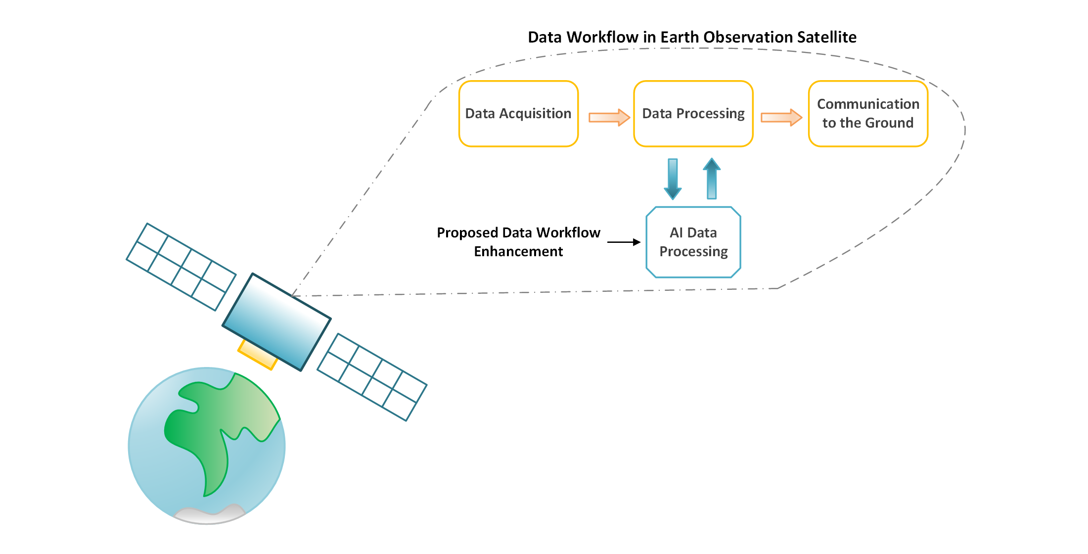
We can easily identify application scenarios that can benefit from running AI algorithms directly on board the satellite. For example, satellite missions that employ nano- and micro-satellites are remote systems with strict HW restrictions on power consumption and processor capability. In Earth Observation (EO) missions, the data workflow usually consists of:
- Data acquisition, for example, hyperspectral or SAR images;
- Data processing, a usually basic operation such as compression of acquired data;
- Data transmission to the ground station;
- Data processing on ground.
The amounts of data acquired can be huge depending on the mission goal and budget [2]. Data transmission (downlink) to the ground station can be very slow due to multiple factors; for example, the low speed of low power–low bandwidth transmitters, and the fact that transmission can usually only be done when the satellite is within the transmission range of the ground station. Downlink problems are gaining attention due to the very large amounts of data that new generation sensors can acquire. Some solutions have already been proposed, and some new communications technology to address downlink problems have been developed [3]. Benefits of applying AI algorithms to these kinds of missions include:
- The ability to remove irrelevant data, for example, cloudy images, before transmission;
- Early notification of interesting events, such as wildfires or oil spills. By running AI on board, the satellite will be able to identify specific situations directly on board and will only need to transmit a notification to the ground.
Such improvements in the data workflow can lead to less waste of time and energy for the satellite and provide early notification for those situations that require timely intervention.
In this paper, we present a Convolutional Neural Network (CNN) architecture for semantically segmenting SAR images into multiple classes that is specifically designed to run on remote embedded systems that have very limited hardware capability and strict limits on power consumption. Our solution has the important advantage of being able to run on remote embedded systems with limited hardware resources while achieving good performance. We achieve this by adopting a design flow that takes into consideration hardware constraints right from the beginning to develop a system with a memory footprint that is as low as possible.
Due to our system’s small memory footprint, it can be run on dedicated HW accelerators on board the satellite, which enables our system to identify oil spills from SAR images in a significantly shorter amount of time.
The main objective of this work is to enable oil spills identification directly on board resource constrained systems, i.e., nano- and micro-satellites, by leveraging dedicated hardware accelerators to achieve low power and low inference time. A CNN model is used to take advantage of commercially available hardware accelerators suitable for space applications. A performance comparison between two different accelerators running the proposed CNN is performed. In addition, a comparison with related works is shown to highlight the strengths and limitations of the proposed solution.
In Section 2, we summarize related work, especially those related to automatic methods for identifying oil spills using CNNs. In Section 3, we will introduce the main embedded devices and HW accelerators available for deploying AI applications directly on board the satellite. In Section 4, we will describe the dataset and the proposed CNN architecture. In Section 5, we will discuss the results obtained in terms of inference time, power consumption, size of the proposed CNN, and we will compare it with state-of-the-art solutions. In Section 6, we will discuss the results. Finally, in Section 7, we will provide conclusions.
2. Related Work
Oil spill detection can be conducted with various methods, ranging from manual to semi-automatic and fully automatic methods. With manual methods, skilled operators analyze images to determine whether dark formations correspond to oil spills or not. With semi-automatic methods, image features related to geometrical characteristics, physical and textural information, and contextual information [4] are used as input to various types of classification systems. In [5], for example, a forest of decision trees was applied to the set of selected features to identify oil spills in satellite images based on the experience of skilled operators. In [6], a set of selected features was used as input to drive an Artificial Neural Network (ANN) able to classify a dark formation as oil spill or look-alike.
CNNs are one of the most widely used models in deep learning [7], and are able to achieve state-of-the-art results in image analysis applications of different areas, i.e., image forensic [8], sea ice detection [9], autonomous navigation [10], and agriculture [11]. They represent a fully automatic way to address the problem of oil spill identification since they do not require a human to define the specific features that are used to classify oil spill and look-alike formations. The relevant features are automatically identified during the CNN training process.
CNNs have been widely used to perform segmentation of SAR images to identify oil spills [12,13,14,15,16,17,18,19,20,21,22,23,24,25]. One example of this approach can be found in [26], where a NN, specifically the Multilayer Perceptron (MLP), was applied to SAR images for the first time. In [27], a CNNs was used to semantically segment the input image and classify each pixel into one of five different classes (Sea, Oil Spill, Look-Alike, Ship, and Land). In [28], the same authors also presented a publicly available dataset consisting of pixel labeled SAR images. In [29], a CNN was used to discriminate oil pixels from background pixels. In [30], a deep learning fusion recognition method was proposed, which achieves good adaptability and robustness when applied to images with a wide range of different attitude angles, backgrounds and noise.
Automatic classification methods consist of one or more stages. Usually, single-stage methods are faster, but achieve lower quality results compared to multistage ones. An example of a single-stage method was proposed in [31], where a CNN (A-ConvNets) performs the classification using SAR images. In [32], a two-stage framework based on two CNNs was proposed to semantically segment SAR images. In [33], the authors presented a three-stage method based on a Mask R-CNN model that is able to identify different Region of Interests (ROIs) and segment them, obtaining state-of-the-art results in terms of classification ability. CNNs are also used to identify oil spills from polarimetric SAR images [34,35,36] and hyperspectral images [37] as well.
3. Boards and Hardware Accelerators for Neural Networks
The main goal of this research activity is to allow AI systems to directly run on embedded devices with limited hardware resources in remote environments, such as satellites that identify oil spills from SAR images. To this end, we need to know which embedded devices are available to run NN inferences, and the strengths and limitations of each of them. Here, we briefly introduce some of the most widely used embedded devices and Commercial Off-The-Shelf (COTS) hardware accelerators specifically meant to run NN inferences.
- Myriad: The Intel Movidius Myriad Vision Processing Units (VPUs) are hardware accelerators able to run NN inferences using processors called Streaming Hybrid Architecture Vector Engines (SHAVEs). Currently, there are two versions of this accelerator: the Myriad 2 [38] and the Myriad X. They show the best performance accelerating NN with convolutional layers, such as Fully Convolutional Network (FCN) and CNN. Their weakness is the limited intralayer memory available, which is about 128 MB. This imposes a severe limit on the size of the output of each layer of the NN that can be deployed on it.
- Google Coral: The Coral Edge Tensor Processing Unit (TPU) is an Application-Specific Integrated Circuit (ASIC) developed by Google with the aim to accelerate TensorFlow Lite models while maintaining a low power consumption. It can perform up to 2 trillion operations per second (TOPS) per watt (W). The Google Coral TPU is available in different form factors. These devices can run inferences of 8-Bit NN and obtains maximum performance when running inferences of FCN. The drawback of these devices is that some NN layers are not supported or only partially supported. For example, at the time this paper is written, the Softmax layer supports only 1D input tensor with a maximum of 16,000 elements. The layers that are not supported can be run outside the accelerator on the host system; this generally leads to lower performance and puts extra load on the host CPU preventing the use of the accelerator when low latency is required.
- Nvidia Jetson Nano: The Nvidia Jetson Nano is a board that features both a Central Processing Unit (CPU) and a Graphic Processing Unit (GPU). It can run an Operating System (OS) and allows execution of many kinds of NNs due to the versatility of the featured GPU. It can work with a maximum power consumption of 5 or 10 W. Its main limitation is the limited amount of RAM it features, which is 4 GB in the largest memory size version. To overcome this limitation TensorFlow Lite can be used which allows one to use less hardware resources during inference time or to even quantize a NN with minor loss of accuracy.
- FPGA: Due to their high flexibility, Field-Programmable Gate Arrays (FPGAs) can theoretically support any layer, provided that a sufficient amount of logical resources are available. The drawback with this technology is that programming FPGAs usually requires specific skills and a longer development time [39,40] especially when compared to COTS devices like the ones mentioned above. It is worth noting that recently some FPGA manufacturers have released tools to help developers deploy NNs on their FPGA boards. These tools usually come with some limitations such as the number of supported layer types. Moreover, FPGAs for which the performance can be compared to the performance of dedicated hardware accelerators are normally more expensive compared to the dedicated hardware accelerators. The cost of FPGAs can also increase when additional special technologies are required, such as when radiation tolerance is required.
3.1. Radiation Hardened Devices
One of the main goals of this work is to be able to run AI systems directly on board satellites. One of the most important requirements for technology used for space applications is the ability to work in an environment with radiation. Radiation can cause different types of errors, for example:
- Single-Event Latch-up (SEL) Linear Energy Transfer (LET). This affects transistor junctions and can have irreversible effects (permanent or hard errors).
- Single-Event Transient (SET). This is a spurious signal produced by radiation; it causes temporary effects (soft errors).
- Single-Event Upset (SEU). This is a change in the state of a memory, it causes temporary effects (soft errors) on the device, but may cause the software to enter into an inconsistent state until a reset is issued.
Embedded devices must guarantee that they can properly work in these environments. The amount of radiation a device can tolerate is indicated as Total Ionizing Dose (TID). Radiation tolerance of a device can be achieved in different ways [41,42,43] and depends on both the design methodology and the technologies used to make them. Examples of devices specifically built to work in space environment include the following:
Concerning COTS HW accelerators, some radiation tests have been conducted both on the Myriad 2 VPU and the Jetson Nano board. The Myriad 2 can be found in many different devices, such as the Eyes of Things (EoT) board [46]. The results obtained shown that the Myriad 2 can tolerate about 49 Krad [47]. For the Jetson Nano preliminary results suggest that it can tolerate about 20 Krad [48]. Results for Myriad 2 and Jeston Nano suggest that they can be employed in short missions, especially those for Low Earth Orbit (LEO) where devices are subjected to less radiation compared with other missions, e.g., Medium Earth Orbit (MEO) and Geosynchronous Equatorial Orbit (GEO) missions. In Table 1, the amount of radiation that the aforementioned devices can tolerate is shown.
3.2. Which Device Should Be Used to Run Our CNN?
As usual, there is no one perfect solution; it depends on the requirements of the application we would like to deploy and the constraints of the problem we need to solve. As already noted, the development of a CNN for an FPGA could require a considerable amount of time; also, this process can differ slightly from one FPGA brand to another. Moreover, in cases where the application scenario requires special technologies, the cost of a suitable FPGA can be very high; for example, in satellite applications where radiation tolerant or hardened FPGAs must be used [49,50]. Furthermore, we needed to rule out Google Coral because it does not support some of the CNN layers that are required by our application.
Considering these constraints, we selected the Intel Movidius Myriad 2 and the Nvidia Jetson Nano as deployment targets for our system: Intel Movidius Myriad 2, because it supports all the layers used to build our CNN, provided that we do not exceed the amount of intralayer memory available; Nvidia Jetson Nano, because of the versatility of the featured GPU and the fact that it is agnostic to the framework used to design and develop the CNN. Our choice also takes into consideration the short deployment time required by these devices. Since Nvidia made an OS with pre-installed GPU drivers available for the Jetson Nano board, it is possible to directly run CNN inferences using the TensorFlow environment. For the Movidius Myriad 2, the target device is the Movidius Neural Compute Stick (NCS), a device that features a Myriad 2 chip and a USB form factor. Once the CNN is deployed on the NCS it can also be used on the EoT board, which has been tested for radiation tolerance. To be able to run a CNN on the Myriad 2, it must be quantized and converted to a specific format. The quantization process converts the weights of the CNN from 32 to 16 bits and can affect the performance of the CNN itself. The conversion can be performed both via the Neural Compute Software Development Kit (NCSDK) [51] or the OpenVINO toolkit [52].
Finally, these two COTS devices represent a desirable choice for satellite applications. The Myriad 2 chip has passed the preliminary radiation tests at CERN [47] and it has already been used in the PhiSat-1 mission [53]. Furthermore, some products of the Nvidia Jetson family are currently being considered for possible use in future missions [54].
4. Methods
4.1. Dataset Description
Although SAR images represent a powerful tool to monitor oil spills, there is a lack of publicly available labeled datasets. This limits the research in this topic area making different studies difficult to compare; especially when AI techniques are involved. To overcome this problem, we used the dataset described in [28]. That dataset consists of SAR images (originally acquired from the Sentinel-1 European Satellite missions) collected via the European Space Agency (ESA) database, the Copernicus Open Access Hub (https://scihub.copernicus.eu/ (accessed on 6 September 2021)), while the location and timestamps of the oil spills were provided by the European Maritime Safety Agency (EMSA) (CleanSeaNet service). Oil spill information refers to pollution phenomena that took place from 28 September 2015 to 31 October 2017. As specified in [28], the SAR images provided in this dataset have been pre-processed by applying radiometric calibration, speckle filtering, and dB to luminosity conversion. These operations are usually affordable in terms of processor capability and energy budget of satellite systems. Considering the case where these operations are not affordable for a specific mission with very low budget, it is probably not worth implementing onboard SAR images processing for this type of mission. Sharing the same dataset allows us to easily compare results from different studies. The dataset comprises 1002 images for the training and validation sets and 110 images for the test set. Each image is (1250, 650) pixels. Since the original image size was too large to fit into a small CNN, we needed to split input images into tiles. We needed to choose a tile size small enough to save memory at inference time while containing as much scene context as possible; hence, we set the input size as (320, 320) pixels. A smaller tile dimension size could lead to poor segmentation results due to the lack of context information. Moreover (320, 320) pixels are the same tile size used in [28] and this allows for an easier comparison between the two solutions. We randomly sampled 6400 tiles for the training set and 1616 for the validation set, while the test set consists of 880 tiles. In the dataset we can find five different object classes, and their labels classify each pixel in the image into one of the following classes:
- Sea;
- Oil spill;
- Look-alike;
- Ship;
- Land.
Look-alike areas are caused by wind and other natural phenomena; they look a lot like oil spills and represent one of the main challenges in any multi-class classification problem that tries to distinguish between these two classes.
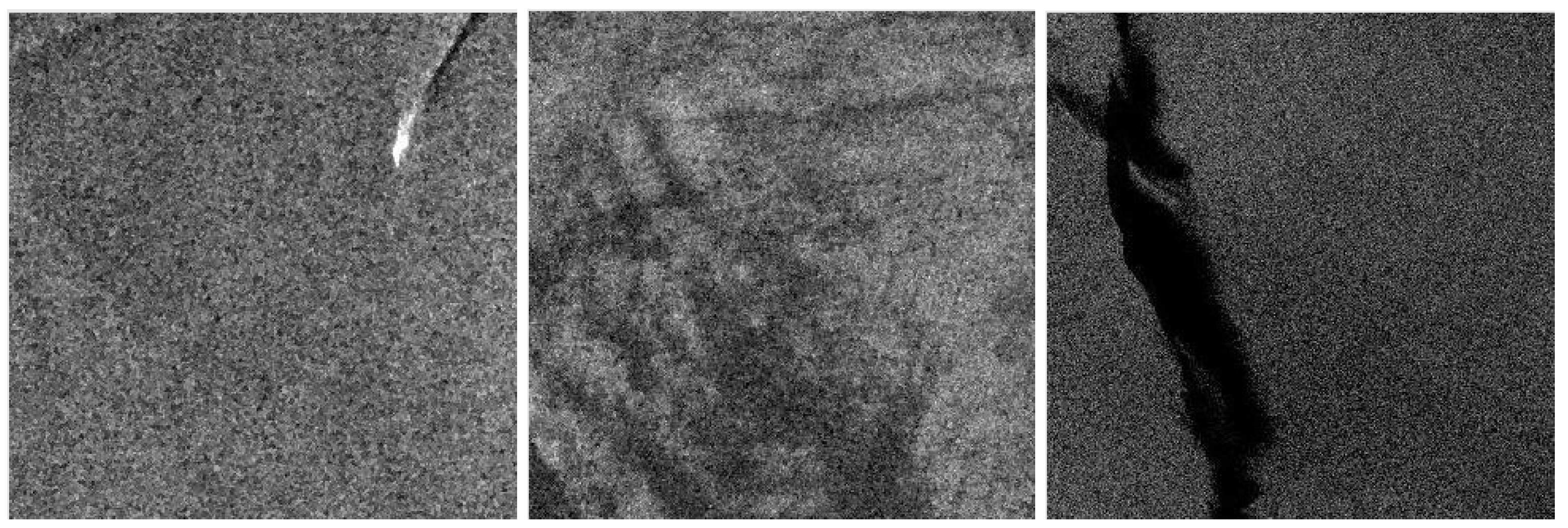
The distribution of the pixels among the classes is shown in Table 2. We can see that there are skew classes, in particular, the Oil Spill class represents only of the entire dataset. This class imbalance represents another challenge since we have very few examples from which our CNN can learn to distinguish between Oil Spill class and other classes. Figure 1 shows three tiles that are used to train the CNN.
4.2. Network Architecture
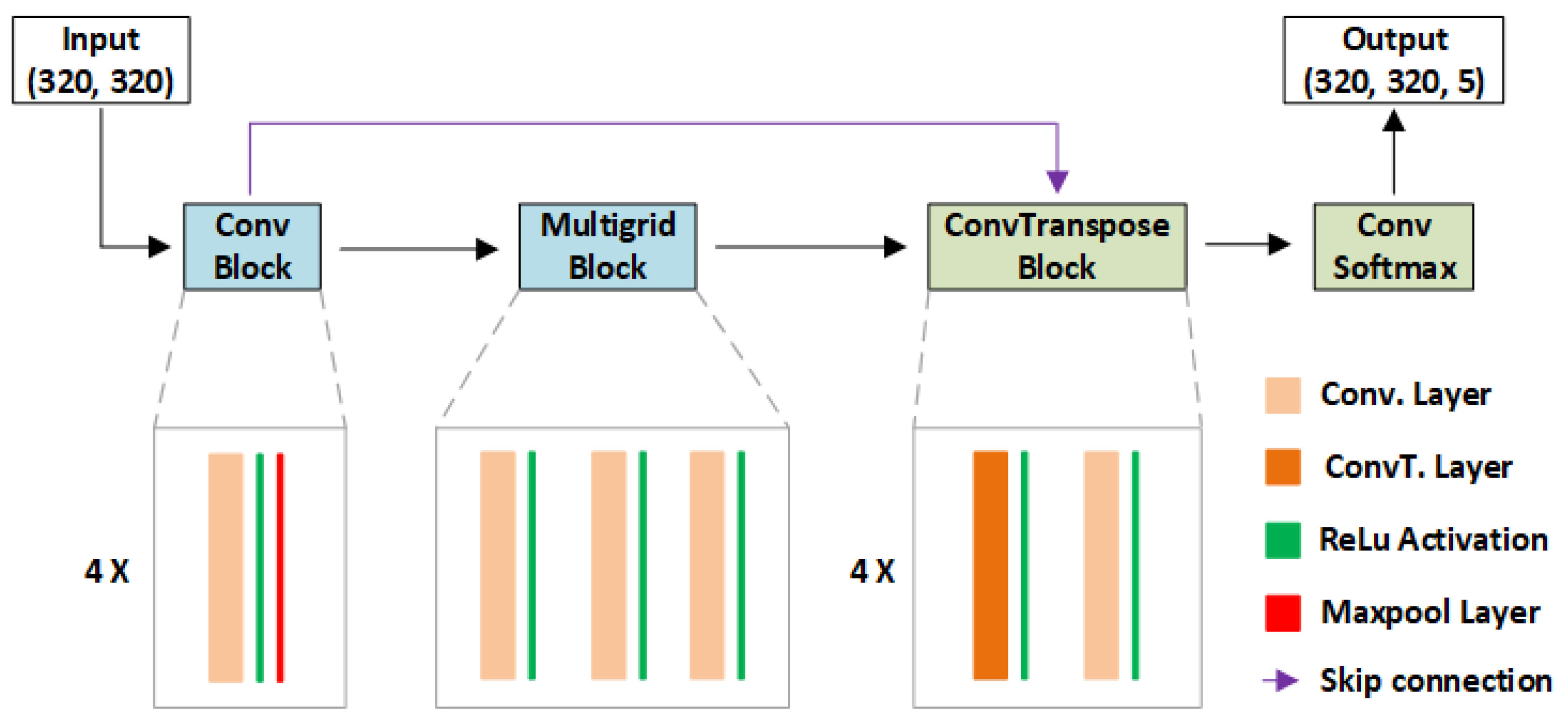
The CNN that we designed and developed consists of two sections: the first section extracts information from the input tile and codes it into an embedding by repeatedly shrinking the feature maps, while the second section up-scales the previously generated embedding up to the original dimension and classifies each pixel of the tile. In Figure 2, blocks with light blue background belong to the first section, while blocks with light green background belongs to the second section. Conv Block contains 4 sub-blocks. Each sub-block consists of a Convolution layer, with 3 × 3 kernel and stride 2, followed by a MaxPooling layer and produces as an output a feature map with an output stride of 2. Since there are 4 sub-blocks inside Conv Block, the feature map obtained as output has an output stride of 16. Multigrid Block employs multiple Convolution layers with different dilation rates, which allow one to control the receptive field without increasing the number of weights of the CNN [55]. In ConvTranspose Block, there are 4 sub-blocks. Each sub-block consists of a transpose convolution and a Convolution layer, used to upscale the feature map by a factor of 2. ConvTranspose Block allows one to upscale the feature maps up to the original dimension of the input tile. A skip connection connects the feature maps from the Conv Block, when output stride is 8, to the ConvTranspose Block to improve the reconstruction of the fine detail during the upscaling process. Finally, a Convolution layer and a Softmax layer are used to generate the output mask. An argmax can be used as a post processing operation to obtain a 2-dimensional mask with the predicted class for each pixel. The proposed CNN is kept as shallow as possible to obtain low inference times even on resource constrained devices. Our CNN employs only four types of layers and two activation functions:
- Convolution;
- Max pooling;
- Transpose convolution;
- Add;
- ReLU and Softmax as activation functions.
These are some of the most common layers used to build CNNs. In this way, we aim to make our CNN model as compliant as possible with the set of layers supported by hardware accelerators currently available on the market.
Techniques like Atrous Spatial Pyramid Pooling (ASPP) [56] and multigrid [57] are not used because they may require a large amount of memory depending on the size of the feature map they need to work on. Other solutions, like [28], use MobileNetV2 [58] as the first section of the CNN. While MobileNetV2 is found to be effective in the feature extraction task, it employs sequences of bottleneck residual blocks that can drastically increase inference time and memory footprint due to the expansion factor used by these blocks. In our solution, dilated convolutions [59] are used since they can increase the receptive field of the filter without requiring additional parameters and thus resources.
4.3. Training Phase
The obtained CNN is a relatively shallow network with a few thousand parameters. This allows one to use a large batch size value without running out of memory during the training phase. We train the CNN on an Nvidia Tesla T4 and we choose a batch size of 32 and Adam [60] as the optimizer. Since our dataset presents a strong foreground–background class imbalance, we use the -balanced version of the focal loss [61], shown in Equation (1), that is found to be effective in handling problems with strong class imbalances.
Focal loss exploits the modulating factor that helps to focus the training process on hard examples. The and parameters can be tuned according to the problem to be solved, while is defined as:
where y is the ground truth class and p is the output of the CNN.
One epoch takes about 90 s on Nvidia Tesla T4 GPU. The duration of the train phase lasts about 270 epochs; at this point, the training process stopped, because the CNN started to overfit on the training set, as shown in Figure 3 where the loss on the training set continued to decrease while the one on the validation set did not.
5. Results
When evaluating the performance of a CNN, previous solutions usually only consider the accuracy and, sometimes, consider the inference time. In order to run CNNs directly on board in embedded systems, we need to consider other parameters, such as power consumption, the amount of hardware resources required, and deployment time. Here, we present the performance of the CNN that we have designed, using the following criteria:
- Intersection over Union (IoU), one of the most used metrics to evaluate the goodness of segmentation CNN;
- Inference time, the time needed to run 1 inference of the proposed CNN on the devices chosen as deployment target;
- Power consumption, an estimate of the power per inference needed on the selected deployment targets;
- Size of the CNN, i.e., the file size of the stored CNN model. This parameter can be of special importance, because many types of remote embedded systems require wireless communication so a smaller file size means less time to deploy the CNN to the system.
5.1. IoU Results
IoU tells us how capable the CNN is in classifying each pixel of the image. It is defined as shown in Equation (3).
Above, A and B are the set of pixels predicted to belong to the output class and the ground truth, respectively. For multi-class problems, the mean IoU can be used to evaluate the overall CNN IoU performance. It consists of the mean of the IoU for each output class, as shown in Equation (4).
Above, n is the number of classes of the problem, is the set of predicted pixels for class ith, and is the set of ground truth pixels for class ith.
Results in terms of IoU are shown in Table 3 for the Nvidia Tesla T4 (where the CNN was trained), the Nvidia Jetson Nano, and the Movidius NCS. We can see that IoUs do not change between the two GPUs, as we can expect, while for the Movidius NCS there is a slight difference for some output classes due to the quantization process mentioned earlier. It must be noted that the mean IoU over all classes is lower than state-of-the-art solutions [33]. This is due to the small number of layers and channels per layer used in our CNN, and the fact that we do not employ strategies that are demanding in terms of memory and inference time.
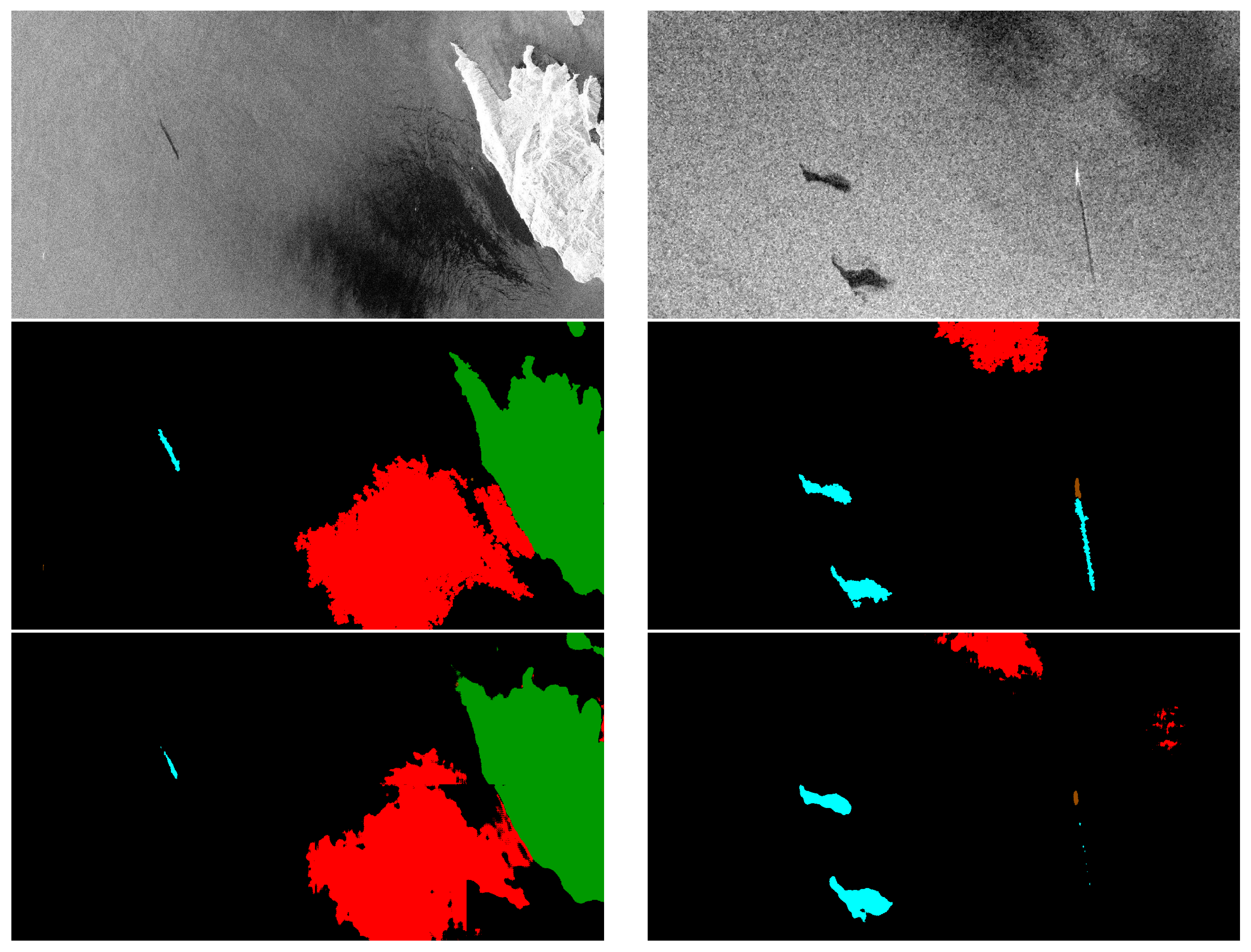
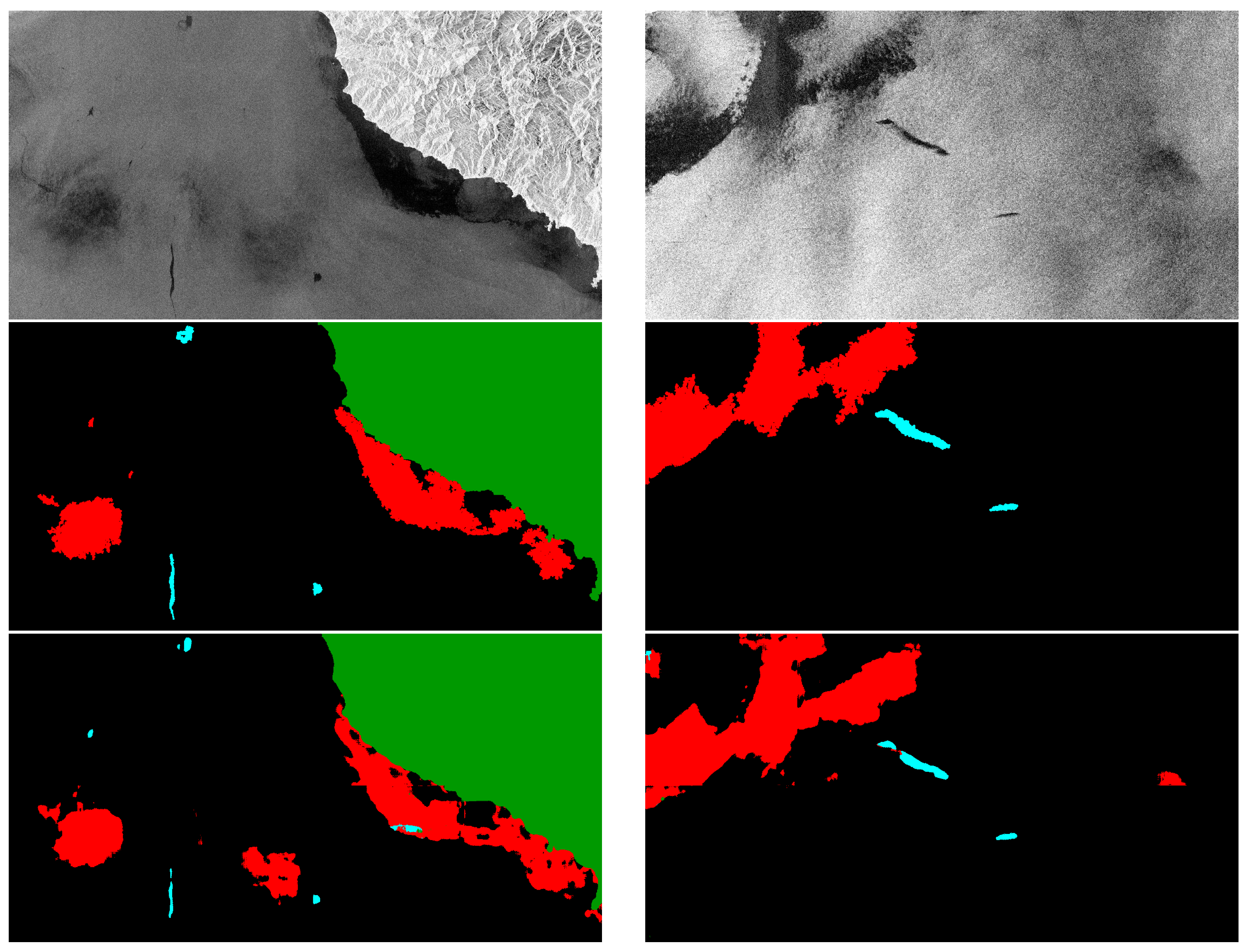
Here five sample images taken from the test set are shown and discussed. For each sample, we show the input SAR image, the ground truth, and the predicted mask obtained from our solution. In the first sample (left column of Figure 4) land, look-alike, and a small oil spill are shown. In this sample, the three classes are recognized, but their shape is not very well defined, especially the border.
In the second sample (right column of Figure 4), two large oil spills on the left, a long oil spill with a ship at its top and a look-alike formation on the top of the image are shown. In this sample, the ship is well recognized, while the thinnest part of the oil spill is not recognized; also, the fine grain details of both oil spills on the left and look-alike are missing. Moreover, some small spots of look-alikes appear in the right of the predicted mask. These spots are False Positive (FP) results and contribute to decreasing the IoU for that class.
The third sample (left column of Figure 5) features three small oil spills, two main look-alike formations, and a big land area on the right. In this case, land is well recognized, while oil spill class shows some FP spots where look-alike areas should appear. Other look-alike areas are recognized except for the fine detail on the border. A look-alike area appears on the bottom of the predicted mask, which represents a FP result.
The fourth sample (right column of Figure 5) features two oil spills in the middle and a huge look-alike formation in the top left. In this case, both classes are well recognized. Only a small portion of misclassified pixels appear as FP results in the predicted mask. We can notice that the predicted mask classifies two dark formations in the top left and the middle right of the image. These two dark areas are also visible in the input images, but are not classified as look-alike in the ground truth mask.
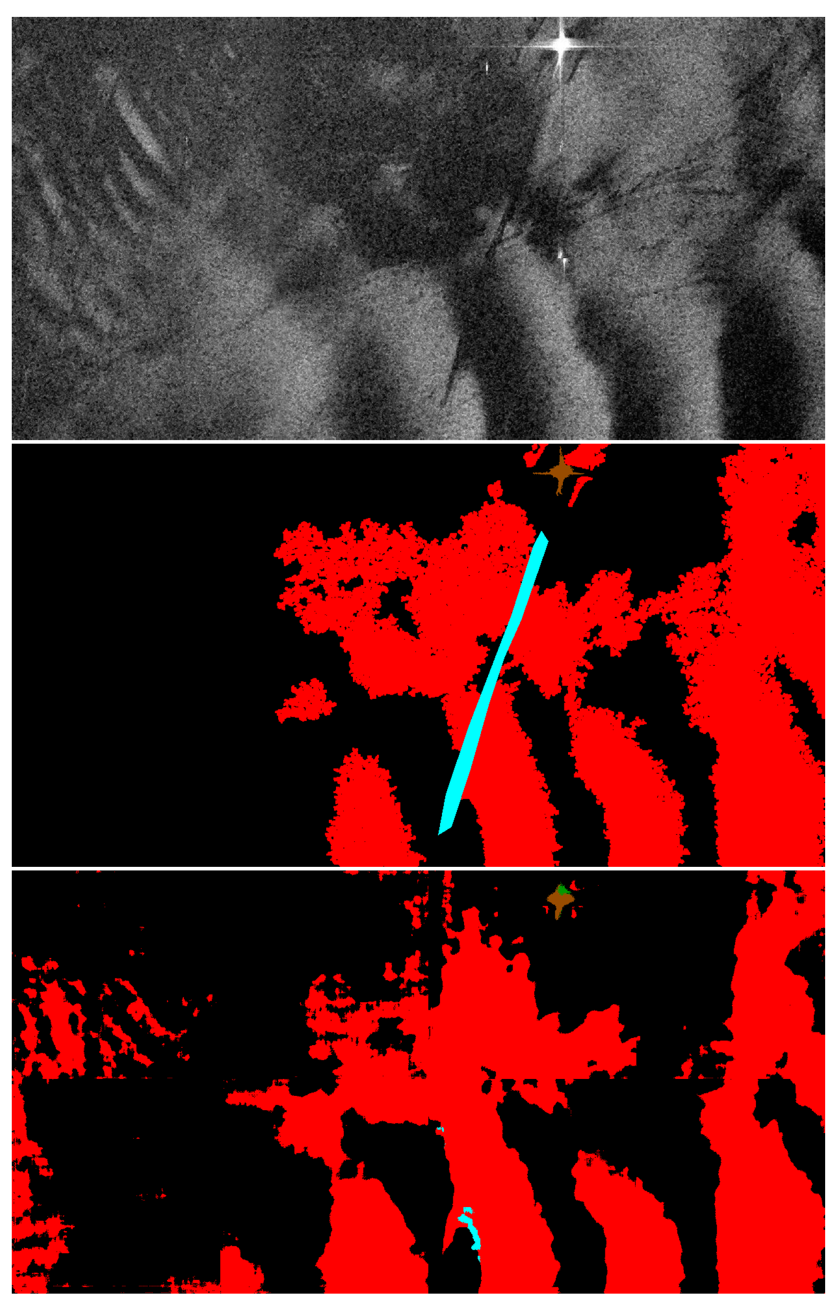
Finally, a non-correct classification is shown in the fifth sample (Figure 6). This sample features a ship on the top, a long oil spill in the middle, and a huge irregular shape look-alike area. Here, the ship is correctly recognized, and the look-alike formation is only partially recognized while the oil spill is completely missing since it is overlapped with the huge look-alike area. There is also a big FP area in the look-alike class on the left of the predicted mask.
5.2. Inference Time Results
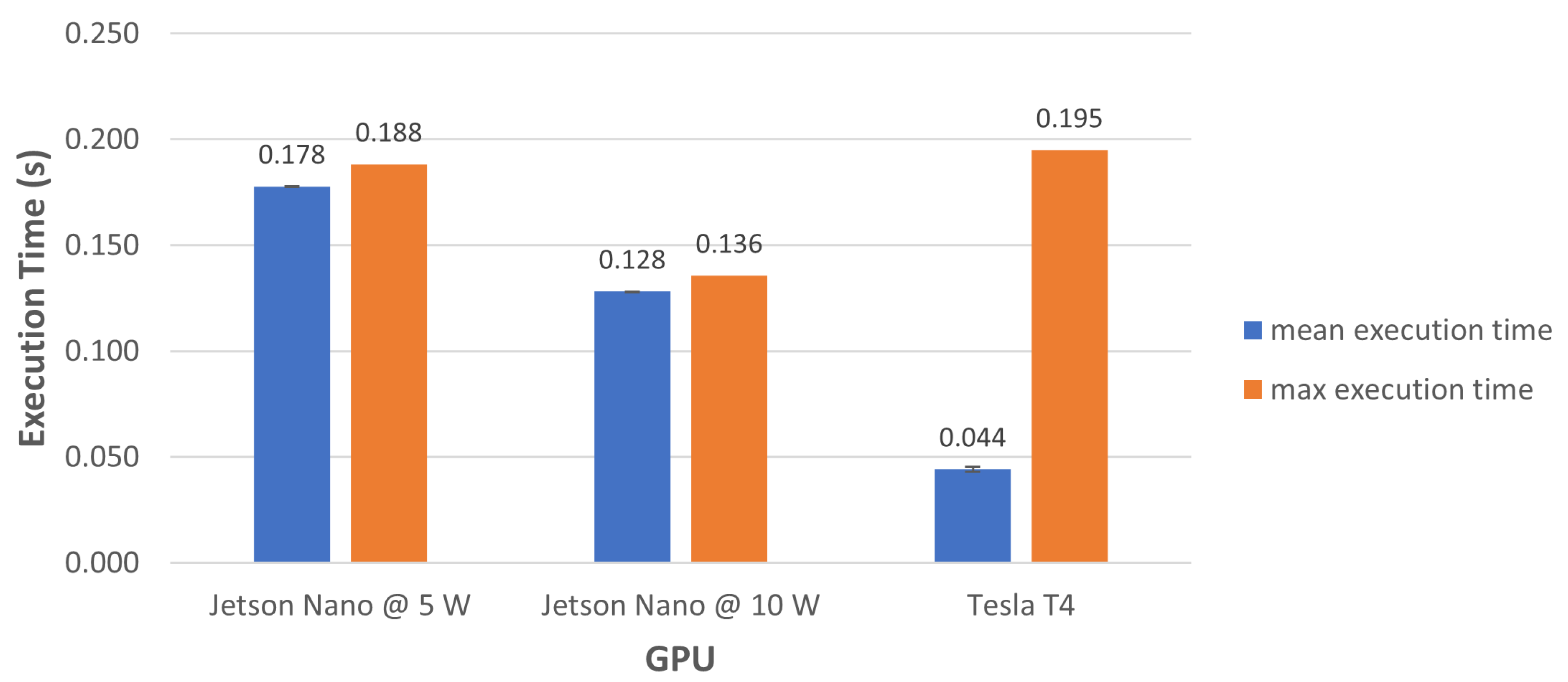
Here, we compare and discuss the inference times of the proposed CNN for the two selected target devices mentioned earlier and for the Nvidia Tesla T4 GPU used to train the CNN. Figure 7 shows inference times for the Nvidia Tesla T4 and Jetson Nano GPUs. For the latter, we can see how power consumption affects the inference time: when power consumption increases from 5 W to 10 W, the inference time decreases by around . Given the small number of parameters of the proposed CNN, the memory footprint depends almost entirely on the framework used to run the inference.
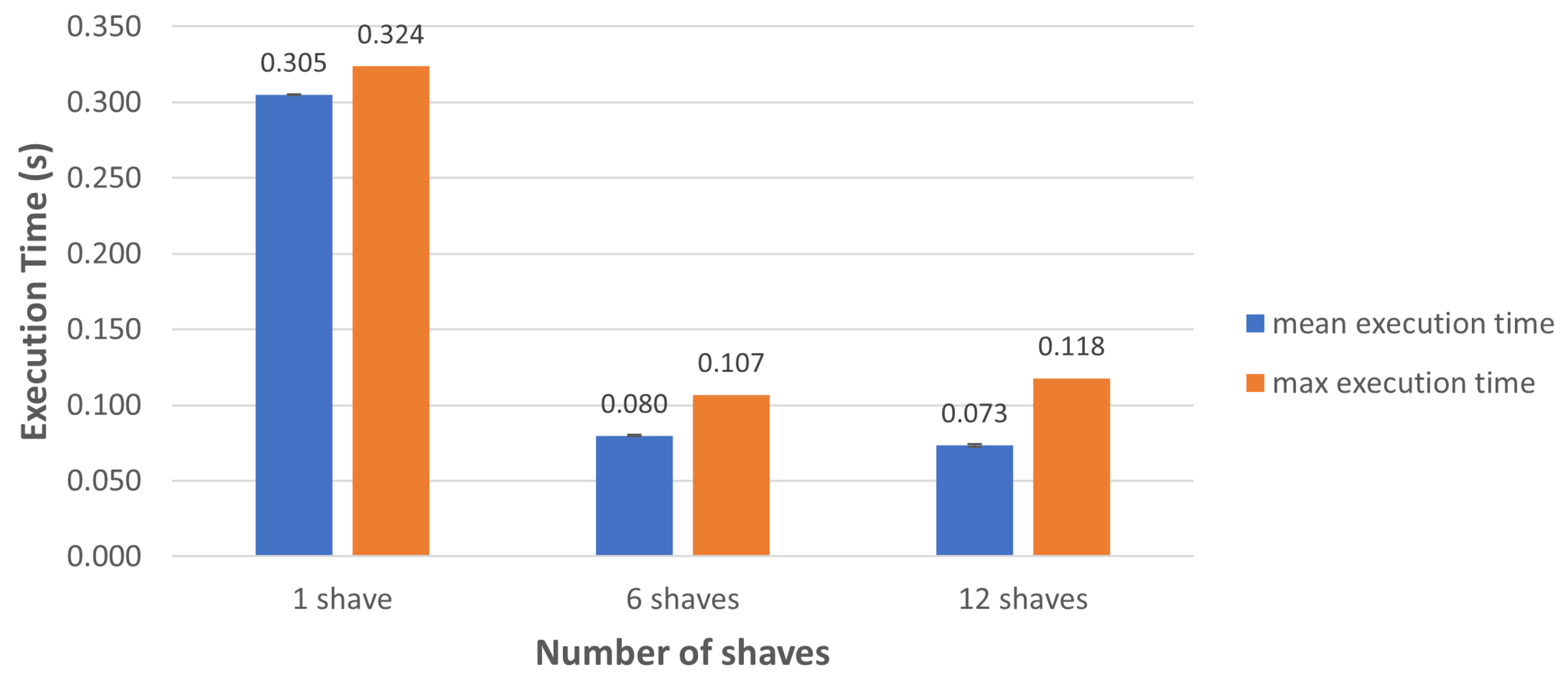
For the Movidius NCS, we run the CNN using different numbers of SHAVEs and different software configurations. The Movidius NCS can work using from 1 to 12 SHAVEs. When only 1 SHAVE is used, the Movidius NCS delivers minimum performance and power consumption; when 12 SHAVEs are used, it delivers maximum performance and power consumption. We choose to evaluate configurations employing 1, 6, and 12 SHAVEs to show when best and worst performance are obtained, and when a balanced configuration between performance and power consumption is achieved. Regarding software configurations, we choose to evaluate our CNN both with and without the final Softmax layer. This decision was made based on two observations. The first observation is that the actual 2D mask of the predicted classes must be obtained through an argmax operation on the CNN output and since the gives the same result as we can safely remove the final Softmax layer during deployment time without any negative impact. The second observation is that in our case the tools provided by NCSDK indicate that the proposed CNN with the Softmax layer cannot be used with the Movidius NCS. This indicates that the output of the CNN with Softmax layer could be incorrect. Using our dataset we did not observe any difference in the output masks generated by the proposed CNN with or without the Softmax layer. Based on these observations, we decided to choose the CNN version without the final Softmax layer to be deployed on the Movidius NCS for real work usage, and to evaluate the performance of both versions of the CNN to show how much the Softmax layer affects the inference time on this device.
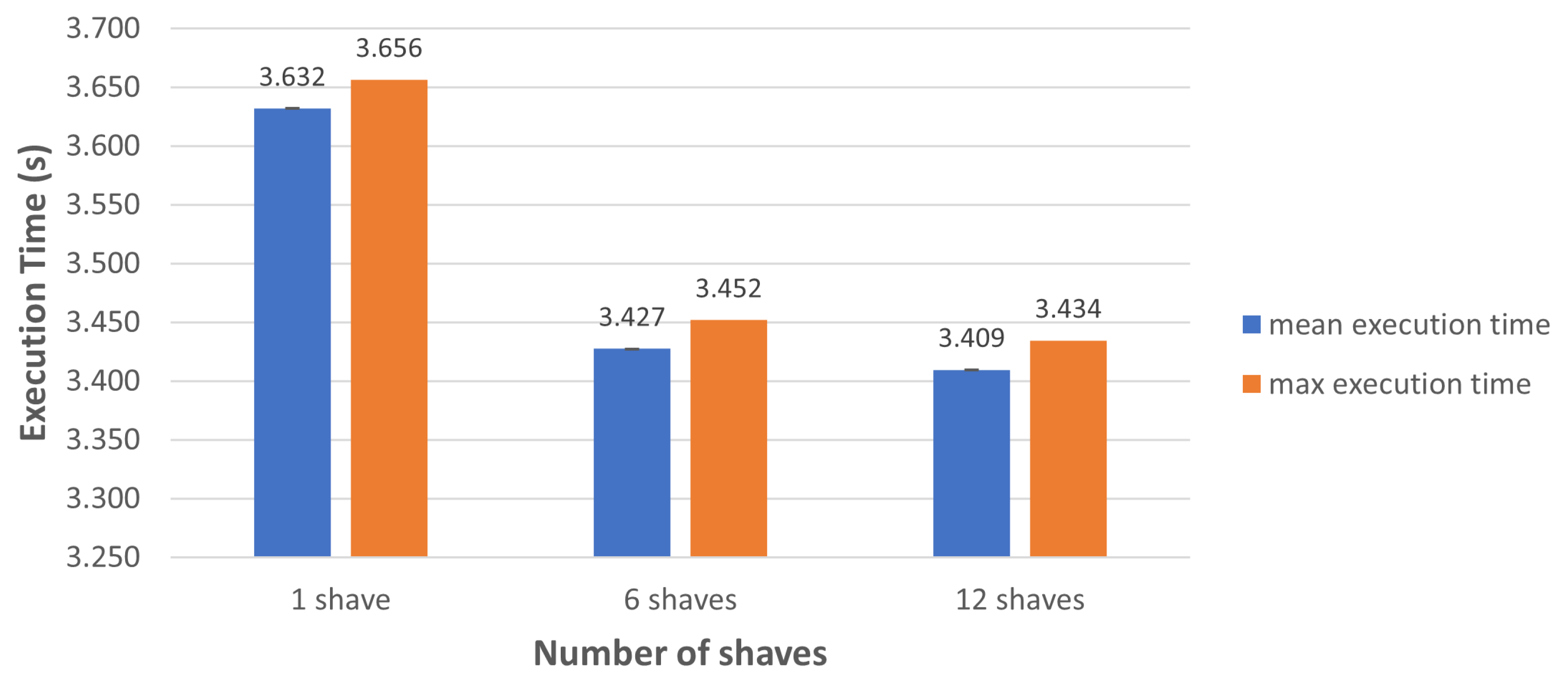
Figure 8 shows the inference times when using 1, 6, and 12 SHAVEs and using the CNN version together with the final Softmax layer. We can see that inference time decreases as the number of SHAVEs used increases. Inference time decreases around s when the number of SHAVEs used increases from 1 to 6, while there is no significant improvement when the number of SHAVEs used increases from 6 to 12.
Figure 9 shows the inference times when using 1, 6, and 12 SHAVEs and when using the CNN version without the final Softmax layer. Furthermore, in this case, inference time decreases as the number of SHAVEs used increases. Inference time decreases from to s, which is times better, when the number of SHAVEs used increase from 1 to 6. As in the previous case, no significant improvement is obtained when the number of SHAVEs used increase to 12.
Analyzing this data, we have come to the conclusion that the presence of the final Softmax layer has a negative impact on the inference time performance. We believe that this shows that the Movidius NCS device is not optimized to perform this type of computation while it is highly effective in accelerating Convolution layers as evidenced by the inference time obtained when the Softmax layer is removed. We believe that this does not mean that the Softmax layer should always not be used when deploying CNN to this device, but only shows that the Softmax layer affects the performance of the system negatively in our particular application. It is worth noting that our particular application requires computing the softmax operation for each pixel of the output mask, that is = 102,400 times each time on 5 values. Another thing we have observed is that the Movidius NCS achieves better inference times compared with the Nvidia Jetson Nano, provided that enough SHAVEs are used.
5.3. Power Consumption Results
Since we are particularly interested in being able to run CNNs in remote embedded systems with limited hardware resources, an important part of this research is to explore various techniques for reducing power consumption. Here, we present an analysis of the target devices’ power consumption when running the proposed CNN model.
As mentioned earlier, the power consumption of the Nvidia Jetson Nano can be set to a max value of 5 W or 10 W using a tool; we saw in Section 5.2 how this affects performance of the proposed CNN model in terms of inference time. The ability to set and know in advance the maximum power consumption of the device can make the task of a system designer much easier.
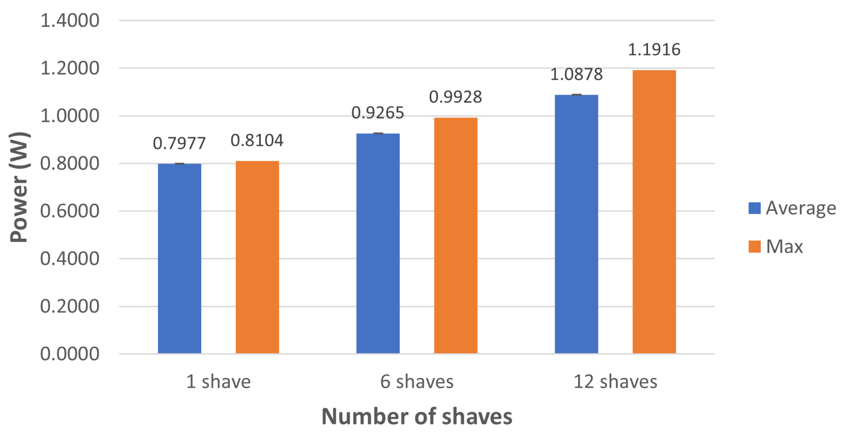
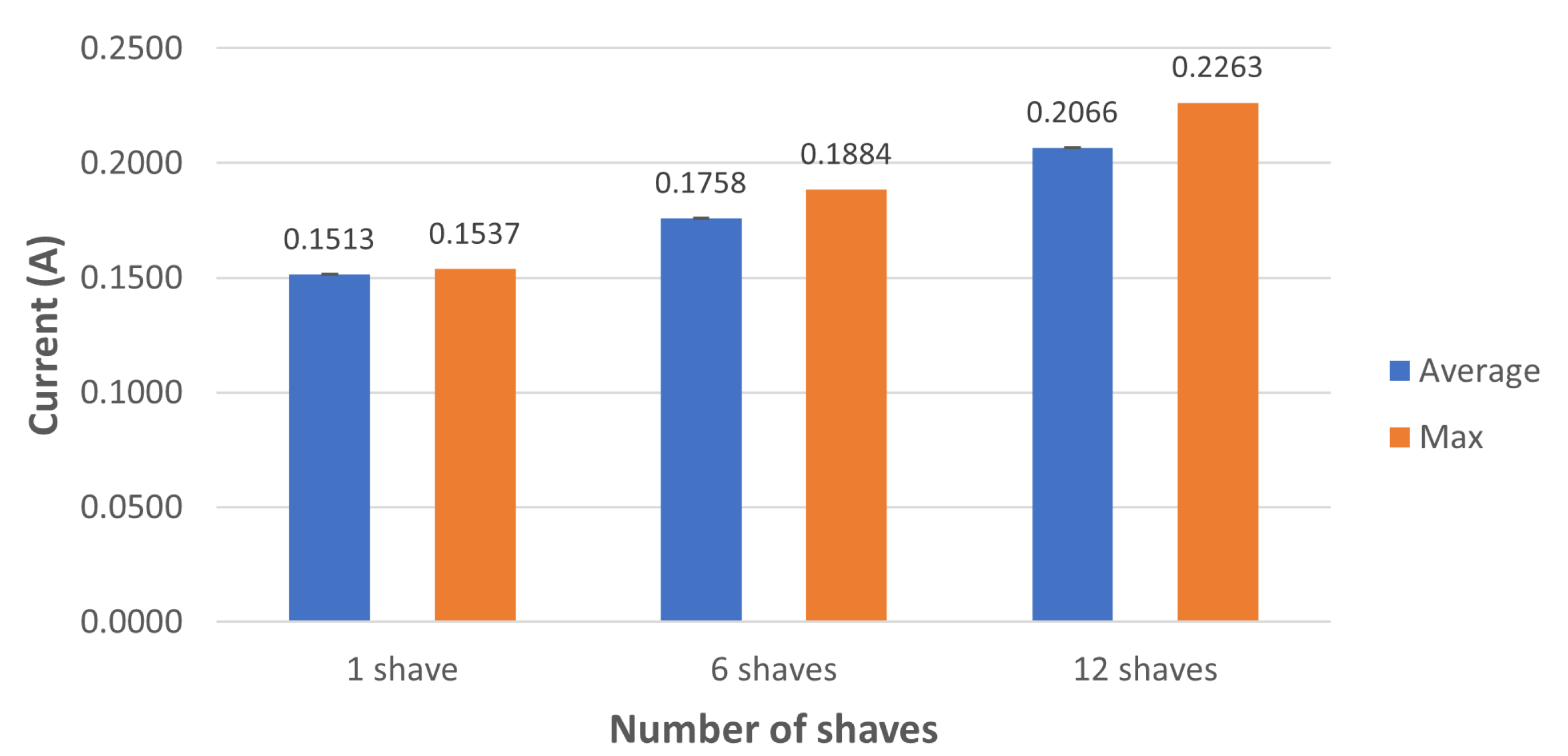
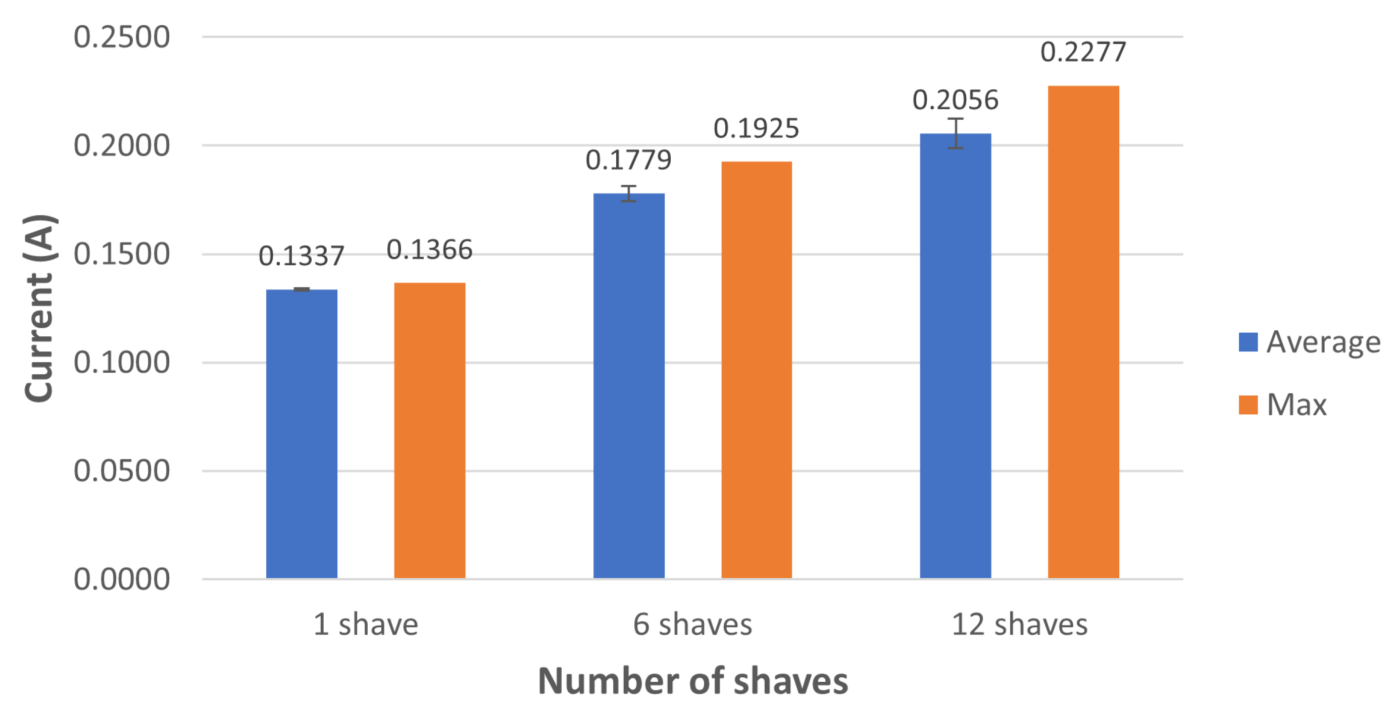
The power consumption of the Movidius NCS depends on how many SHAVEs are used during the inference process. This parameter must be set during the quantization operation. Monitoring the power consumption on the USB port where the NCS was connected can give an estimation of how much power the device requires during the inference process. This setup allows one to monitor how much current is consumed in addition to the power consumption. To obtain a meaningful estimation for the power consumption per inference, we used the average of the power consumption measured over 1000 inferences; the same procedure was also used for estimating the current consumption. For inference time evaluation, we repeat this procedure using 1, 6, and 12 SHAVEs. We evaluated the proposed CNN both with and without the Softmax as the last layer. The 1, 6, and 12 SHAVEs average and maximum values for current and power consumption are shown in Figure 10 and Figure 11, respectively. We note that increasing the SHAVEs used from 1 to 6 leads to an increase of about ∼1.16 times for current and power consumption, and increasing the SHAVEs used from 6 to 12 SHAVEs results in an increase of ∼1.17 times for the same quantities. We can note similar behavior when the final Softmax layer is not used as shown by the power and current consumption shown in Figure 12 and Figure 13, respectively. The only noticeable difference occurs only when 1 SHAVE is used; in that case the CNN version without the Softmax layer has slightly lower consumption.
These results must be considered in combination with the inference time, which has been analyzed in Section 5.2, to assess the total energy consumption required by the CNN model. This way the balance between consumption and performance can be tuned according to the energy budget of the entire system; that is a crucial factor when designing embedded systems for remote missions.
5.4. CNN Size
In the past, CNN designers and developers have paid very little attention to this issue, but now this issue is gaining more and more importance and attention, because in many CNN applications, one needs to take into consideration the ability to reconfigure remote systems after their deployment. Reconfiguration during a satellite’s lifetime can occur when updating the software becomes necessary, due to bugs or the need to upgrade performance with new algorithms, or to re-target the mission when a previous goal has been completed and the satellite can still operate properly. In these situations, the amount of time needed to develop the new software (train the CNN in our case) and transmit it to the remote system needs to be reduced as much as possible, since it represents a significant cost for the entire mission. For example, for satellite systems, efficient use of bandwidth is extremely important, especially for low budget–low power missions such as nano- and micro-satellites used for remote sensing that cannot afford to use expensive transmission systems with high bandwidth. Furthermore, satellites can send/receive data only when they are in the line of sight with a ground station.
We can now see the value of a CNN with a small number of parameters that reduce training times, compared to bigger CNNs with a very large number of parameters, and the value of a small file size, which enables system reconfiguration with affordable cost in terms of bandwidth and time needed for the transmission of the file itself. As shown in Table 4, the proposed CNN can be stored in about 270 KB for the Nvidia Jetson Nano, and only 20 KB is required for the Movidius NCS.
5.5. Comparison with Related Work
Here we summarize the results of the proposed CNN compared with similar solutions from related work highlighting its strengths and limitations. Table 5 shows results in terms of performance, memory footprint, inference time, and the number of stages of related work, in particular those involving NNs. Compared with related work that reports memory footprint and inference time, our solution exhibits a significant advantage regarding these two metrics, even though it achieves a lower mean IoU as already explained in previous sections.
Since both our solution and the one proposed in [28] are single-stage methods based on CNN, share the same dataset, and have the same goal of semantically segmenting images into five different classes, it is possible to make meaningful comparisons between them. When comparing these two CNNs, the proposed CNN consists of only K parameters, is 200 times smaller, can run an inference in about 73 ms, is times faster, when run on a dedicated hardware accelerator with a power consumption of about W and a negligible memory footprint.
A similar comparison can also be made with [34], even if in this case the difference in the adopted approach and dataset between the two solutions make the comparison less meaningful. Comparison with other solutions is more difficult due to the lack of data in terms of inference time and memory footprint.
6. Discussion
As shown in Table 3, the main reason that the Mean IoU of our CNN is slightly lower than the CNNs that achieved state-of-the-art accuracy is because of the design choices in the CNN architecture that we have adopted in order to reduce the memory footprint, power consumption, and time usage during both training and inference phases. The restrictions that we have adopted include:
- Reduced number of layers. Our CNN is designed to be as shallow as possible;
- Reduced number of channels in each layer to reduce the amount of memory used to store intermediate results;
- Avoidance of the use of memory hungry techniques, such as ASPP;
- Use of layer types commonly supported by most hardware accelerators and COTS devices. This choice aims to develop a CNN compatible with most hardware accelerators available on the market.
As we can see in the results shown in Section 5, one of the most noticeable limitations of our solution is the lack of fine grain detail that can be explained by the restrictions adopted in the CNN architecture. Moreover, the proposed CNN does not perform well in all scenarios included in the test set. When challenging scenarios are detected, i.e., images with high numbers of both oil spills and look-alikes, more in-depth analysis may be required to accurately discriminate between these two classes. A post-processing can be applied to the output of the proposed CNN to identify these situations and send the selected images to the ground. This kind of post-processing can be done by simply counting the oil spill and look-alike pixels in the output masks produced by the proposed CNN. The cost in terms of processor capability is considered affordable as it is not higher than that of the pre-processing operations mentioned in Section 4.1.
On the other hand, our solution exhibits low inference time, a negligible memory footprint, and low power consumption when deployed on dedicated hardware accelerators. Even if this solution does not break new ground in terms of results accuracy, it has the very important advantage of being suitable for embedded applications such as satellite used for remote sensing where low power consumption, short inference time and small memory footprint are major requirements. Moreover, due to the small file size, it is possible to upload an updated version of the CNN to the remote system with significantly less effort, enabling mission goal re-targeting during the mission lifetime.
Solutions like the one presented in this paper can be used to process SAR images to identify relevant phenomena directly on board the satellite and transmit only the results of the processing of SAR images to ground. This can contribute to save bandwidth, transmission time, and reduce power consumption, and effectively reduce the overall mission cost. Other applications include illegal bilge dumping; this can be carried out by post-processing the output of the proposed CNN to correlate the position of a ship and an oil spill when both are detected in the same SAR image. If a correlation is found, the specific SAR image can be sent to the ground for further analysis. This kind post-processing, i.e., measuring the distance between a ship and an oil spill, should not require more compute capability than the other pre- and post-processing operation mentioned earlier.
7. Conclusions
Nowadays, SAR images are widely used to monitor marine ecosystems and to identify oil spills. In recent years, AI solutions, especially CNNs, have gained much greater visibility due to their ability to automatically identify features from images. This has encouraged the development of CNN-based applications to identify oil spills, and in some cases other features, from SAR images. In the past, such applications often rely on general purpose CNNs designed to be deployed on desktop or server machines and were developed using result accuracy performance as the sole criteria, which means that they seldom take possible constraints on hardware resources into consideration. As a result, previous CNN solutions are most often not suitable for embedded devices that cannot afford to use large amounts of expensive hardware resources. Any CNN solution that is meant to run on embedded devices must address these limitations in its early design stages. Our solution is meant to be useful for embedded devices used in remote environments that have very limited hardware resources and that require very low power consumption. Remote embedded systems, such as satellites used for oil spill identification from SAR images, can benefit from this work by running AI algorithms directly on board so that the amount of data that needs to be transmitted to ground and processed on ground can be reduced, which will be greatly beneficial in reducing the amount of time needed for identification of oil spills from SAR images. The proposed CNN consist of K parameters, exhibits an inference time of 73 ms, a power consumption of W, and a negligible memory footprint. The ability of the proposed CNN to run on the Nvidia Jetson Nano and the Movidius NCS, featuring the Myriad 2 VPU, make it very suitable for use in missions employing those devices, such as short-duration LEO missions.
Author Contributions
Conceptualization, L.D.; formal analysis, L.D.; investigation, L.D.; methodology, L.D.; project administration, L.F.; supervision, J.X. and L.F.; writing—original draft, L.D.; writing—review and editing, J.X. and L.F. All authors have read and agreed to the published version of the manuscript.
Funding
This work has been partially funded by the European Union’s Horizon 2020 innovation action under grant agreement number 761349, TETRAMAX (Technology Transfer via Multinational Application Experiments).
Institutional Review Board Statement
Not applicable.
Informed Consent Statement
Not applicable.
Data Availability Statement
Information on the dataset used in this study can be found at: https://mklab.iti.gr/results/oil-spill-detection-dataset/ (accessed on 6 September 2021). This paper contains modified Copernicus Sentinel data.
Acknowledgments
We would like to thank Sabina Manca, Helen Balderama, Beth Alaksa, and Glenda Lowndes for their administrative support.
Conflicts of Interest
The authors declare no conflict of interest.
References
- Shi, W.; Cao, J.; Zhang, Q.; Li, Y.; Xu, L. Edge Computing: Vision and Challenges. IEEE Internet Things J. 2016, 3, 637–646. [Google Scholar] [CrossRef]
- Liu, P. A survey of remote-sensing big data. Front. Environ. Sci. 2015, 3, 45. [Google Scholar] [CrossRef] [Green Version]
- King, J.; Ness, J.; Bonin, G.; Brett, M.; Faber, D. Nanosat Ka-band communications-A paradigm shift in small satellite data throughput. In Proceedings of the AIAA/USU Conference on Small Satellites, Small But Mighty, SSC12-VI-54; 2012. Available online: https://digitalcommons.usu.edu/smallsat/2012/all2012/54/ (accessed on 6 September 2021).
- Solberg, A.H.; Brekke, C.; Husoy, P.O. Oil spill detection in Radarsat and Envisat SAR images. IEEE Trans. Geosci. Remote Sens. 2007, 45, 746–755. [Google Scholar] [CrossRef]
- Topouzelis, K.; Psyllos, A. Oil spill feature selection and classification using decision tree forest on SAR image data. ISPRS J. Photogramm. Remote Sens. 2012, 68, 135–143. [Google Scholar] [CrossRef]
- Singha, S.; Bellerby, T.J.; Trieschmann, O. Satellite oil spill detection using artificial neural networks. IEEE J. Sel. Top. Appl. Earth Obs. Remote Sens. 2013, 6, 2355–2363. [Google Scholar] [CrossRef]
- Gu, J.; Wang, Z.; Kuen, J.; Ma, L.; Shahroudy, A.; Shuai, B.; Liu, T.; Wang, X.; Wang, G.; Cai, J.; et al. Recent advances in convolutional neural networks. Pattern Recognit. 2018, 77, 354–377. [Google Scholar] [CrossRef] [Green Version]
- Mandelli, S.; Cozzolino, D.; Bestagini, P.; Verdoliva, L.; Tubaro, S. CNN-Based Fast Source Device Identification. IEEE Signal Process. Lett. 2020, 27, 1285–1289. [Google Scholar] [CrossRef]
- Yan, Q.; Huang, W. Sea Ice Sensing From GNSS-R Data Using Convolutional Neural Networks. IEEE Geosci. Remote Sens. Lett. 2018, 15, 1510–1514. [Google Scholar] [CrossRef]
- Li, J.; Yin, J.; Deng, L. A robot vision navigation method using deep learning in edge computing environment. EURASIP J. Adv. Signal Process. 2021, 2021, 1–20. [Google Scholar] [CrossRef]
- Turkoglu, M.O.; D’Aronco, S.; Perich, G.; Liebisch, F.; Streit, C.; Schindler, K.; Wegner, J.D. Crop mapping from image time series: Deep learning with multi-scale label hierarchies. Remote Sens. Environ. 2021, 264, 112603. [Google Scholar] [CrossRef]
- de Souza, D.L.; Neto, A.D.; da Mata, W. Intelligent system for feature extraction of oil slick in sar images: Speckle filter analysis. In Proceedings of the International Conference on Neural Information Processing, Hong Kong, China, 3–6 October 2006; Springer: Berlin/Heidelberg, Germany, 2006; pp. 729–736. [Google Scholar]
- Topouzelis, K.; Karathanassi, V.; Pavlakis, P.; Rokos, D. Detection and discrimination between oil spills and look-alike phenomena through neural networks. ISPRS J. Photogramm. Remote Sens. 2007, 62, 264–270. [Google Scholar] [CrossRef]
- Song, D.; Ding, Y.; Li, X.; Zhang, B.; Xu, M. Ocean oil spill classification with RADARSAT-2 SAR based on an optimized wavelet neural network. Remote Sens. 2017, 9, 799. [Google Scholar] [CrossRef] [Green Version]
- Orfanidis, G.; Ioannidis, K.; Avgerinakis, K.; Vrochidis, S.; Kompatsiaris, I. A deep neural network for oil spill semantic segmentation in SAR images. In Proceedings of the 2018 25th IEEE International Conference on Image Processing (ICIP), Athens, Greece, 7–10 October 2018; pp. 3773–3777. [Google Scholar]
- Nieto-Hidalgo, M.; Gallego, A.J.; Gil, P.; Pertusa, A. Two-stage convolutional neural network for ship and spill detection using SLAR images. IEEE Trans. Geosci. Remote Sens. 2018, 56, 5217–5230. [Google Scholar] [CrossRef] [Green Version]
- Yu, X.; Zhang, H.; Luo, C.; Qi, H.; Ren, P. Oil spill segmentation via adversarial f-divergence learning. IEEE Trans. Geosci. Remote Sens. 2018, 56, 4973–4988. [Google Scholar] [CrossRef]
- Jiao, Z.; Jia, G.; Cai, Y. A new approach to oil spill detection that combines deep learning with unmanned aerial vehicles. Comput. Ind. Eng. 2019, 135, 1300–1311. [Google Scholar] [CrossRef]
- Guo, H.; Wei, G.; An, J. Dark Spot Detection in SAR Images of Oil Spill Using Segnet. Appl. Sci. 2018, 8, 2670. [Google Scholar] [CrossRef] [Green Version]
- Zeng, K.; Wang, Y. A Deep Convolutional Neural Network for Oil Spill Detection from Spaceborne SAR Images. Remote Sens. 2020, 12, 1015. [Google Scholar] [CrossRef] [Green Version]
- Yekeen, S.; Balogun, A. Automated Marine Oil Spill Detection Using Deep Learning Instance Segmentation Model. Int. Arch. Photogramm. Remote Sens. Spat. Inf. Sci. 2020, 43, 1271–1276. [Google Scholar] [CrossRef]
- Bianchi, F.M.; Espeseth, M.M.; Borch, N. Large-Scale Detection and Categorization of Oil Spills from SAR Images with Deep Learning. Remote Sens. 2020, 12, 2260. [Google Scholar] [CrossRef]
- Baek, W.K.; Jung, H.S.; Kim, D. Oil spill detection of Kerch strait in November 2007 from dual-polarized TerraSAR-X image using artificial and convolutional neural network regression models. J. Coast. Res. 2020, 102, 137–144. [Google Scholar] [CrossRef]
- Chen, G.; Li, Y.; Sun, G.; Zhang, Y. Application of Deep Networks to Oil Spill Detection Using Polarimetric Synthetic Aperture Radar Images. Appl. Sci. 2017, 7, 968. [Google Scholar] [CrossRef]
- Gallego, A.J.; Gil, P.; Pertusa, A.; Fisher, R.B. Segmentation of Oil Spills on Side-Looking Airborne Radar Imagery with Autoencoders. Sensors 2018, 18, 797. [Google Scholar] [CrossRef] [Green Version]
- Del Frate, F.; Petrocchi, A.; Lichtenegger, J.; Calabresi, G. Neural networks for oil spill detection using ERS-SAR data. IEEE Trans. Geosci. Remote Sens. 2000, 38, 2282–2287. [Google Scholar] [CrossRef] [Green Version]
- Krestenitis, M.; Orfanidis, G.; Ioannidis, K.; Avgerinakis, K.; Vrochidis, S.; Kompatsiaris, I. Early identification of oil spills in satellite images using deep CNNs. In Proceedings of the International Conference on Multimedia Modeling, Thessaloniki, Greece, 8–11 January 2019; Springer: Berlin/Heidelberg, Germany, 2019; pp. 424–435. [Google Scholar]
- Krestenitis, M.; Orfanidis, G.; Ioannidis, K.; Avgerinakis, K.; Vrochidis, S.; Kompatsiaris, I. Oil Spill Identification from Satellite Images Using Deep Neural Networks. Remote Sens. 2019, 11, 1762. [Google Scholar] [CrossRef] [Green Version]
- Cantorna, D.; Dafonte, C.; Iglesias, A.; Arcay, B. Oil spill segmentation in SAR images using convolutional neural networks. A comparative analysis with clustering and logistic regression algorithms. Appl. Soft Comput. 2019, 84, 105716. [Google Scholar] [CrossRef]
- Jia, Z.; Guangchang, D.; Feng, C.; Xiaodan, X.; Chengming, Q.; Lin, L. A deep learning fusion recognition method based on SAR image data. Procedia Comput. Sci. 2019, 147, 533–541. [Google Scholar] [CrossRef]
- Chen, S.; Wang, H.; Xu, F.; Jin, Y.Q. Target classification using the deep convolutional networks for SAR images. IEEE Trans. Geosci. Remote Sens. 2016, 54, 4806–4817. [Google Scholar] [CrossRef]
- Shaban, M.; Salim, R.; Abu Khalifeh, H.; Khelifi, A.; Shalaby, A.; El-Mashad, S.; Mahmoud, A.; Ghazal, M.; El-Baz, A. A Deep-Learning Framework for the Detection of Oil Spills from SAR Data. Sensors 2021, 21, 2351. [Google Scholar] [CrossRef] [PubMed]
- Temitope Yekeen, S.; Balogun, A.; Wan Yusof, K.B. A novel deep learning instance segmentation model for automated marine oil spill detection. ISPRS J. Photogramm. Remote Sens. 2020, 167, 190–200. [Google Scholar] [CrossRef]
- Zhang, J.; Feng, H.; Luo, Q.; Li, Y.; Wei, J.; Li, J. Oil Spill Detection in Quad-Polarimetric SAR Images Using an Advanced Convolutional Neural Network Based on SuperPixel Model. Remote Sens. 2020, 12, 944. [Google Scholar] [CrossRef] [Green Version]
- Guo, H.; Wu, D.; An, J. Discrimination of Oil Slicks and Lookalikes in Polarimetric SAR Images Using CNN. Sensors 2017, 17, 1837. [Google Scholar] [CrossRef] [PubMed] [Green Version]
- Song, D.; Zhen, Z.; Wang, B.; Li, X.; Gao, L.; Wang, N.; Xie, T.; Zhang, T. A Novel Marine Oil Spillage Identification Scheme Based on Convolution Neural Network Feature Extraction From Fully Polarimetric SAR Imagery. IEEE Access 2020, 8, 59801–59820. [Google Scholar] [CrossRef]
- Liu, B.; Li, Y.; Li, G.; Liu, A. A Spectral Feature Based Convolutional Neural Network for Classification of Sea Surface Oil Spill. ISPRS Int. J. Geo-Inf. 2019, 8, 160. [Google Scholar] [CrossRef] [Green Version]
- Barry, B.; Brick, C.; Connor, F.; Donohoe, D.; Moloney, D.; Richmond, R.; O’Riordan, M.; Toma, V. Always-on vision processing unit for mobile applications. IEEE Micro 2015, 35, 56–66. [Google Scholar] [CrossRef]
- Dinelli, G.; Meoni, G.; Rapuano, E.; Benelli, G.; Fanucci, L. An FPGA-based hardware accelerator for CNNs using on-chip memories only: Design and benchmarking with intel movidius neural compute stick. Int. J. Reconfigurable Comput. 2019, 2019, 7218758. [Google Scholar] [CrossRef] [Green Version]
- Rapuano, E.; Meoni, G.; Pacini, T.; Dinelli, G.; Furano, G.; Giuffrida, G.; Fanucci, L. An FPGA-Based Hardware Accelerator for CNNs Inference on Board Satellites: Benchmarking with Myriad 2-Based Solution for the CloudScout Case Study. Remote Sens. 2021, 13, 1518. [Google Scholar] [CrossRef]
- Liu, G.; Yu, Z.; Xiao, Z.; Wei, J.; Li, B.; Cao, L.; Song, S.; Zhao, W.; Sun, J.; Wang, H. Reliable and Radiation-Hardened Push-Pull pFlash Cell for Reconfigured FPGAs. IEEE Trans. Device Mater. Reliab. 2021, 21, 87–95. [Google Scholar] [CrossRef]
- Shen, C.; Liang, N. Research on anti-SEU strategy for remote sensing camera based on SRAM-FPGA. In Proceedings of the Seventh Symposium on Novel Photoelectronic Detection Technology and Applications, Kunming, China, 12 March 2021; International Society for Optics and Photonics: Bellingham, WA, USA, 2021; Volume 11763, p. 1176308. [Google Scholar]
- Marques, I.; Rodrigues, C.; Tavares, A.; Pinto, S.; Gomes, T. Lock-V: A heterogeneous fault tolerance architecture based on Arm and RISC-V. Microelectron. Reliab. 2021, 120, 114120. [Google Scholar] [CrossRef]
- Rezzak, N.; Wang, J.J.; Dsilva, D.; Jat, N. TID and SEE Characterization of Microsemi’s 4th Generation Radiation Tolerant RTG4 Flash-Based FPGA. In Proceedings of the 2015 IEEE Radiation Effects Data Workshop (REDW), Boston, MA, USA, 13–17 July 2015; pp. 1–6. [Google Scholar]
- GR740-RADS. GR740 Radiation Summary. 2019. Available online: https://www.gaisler.com/doc/gr740/GR740-RADS-1-1-3_GR740_Radiation_Summary.pdf (accessed on 6 September 2021).
- Deniz, O.; Vallez, N.; Espinosa-Aranda, J.L.; Rico-Saavedra, J.M.; Parra-Patino, J.; Bueno, G.; Moloney, D.; Dehghani, A.; Dunne, A.; Pagani, A.; et al. Eyes of things. Sensors 2017, 17, 1173. [Google Scholar] [CrossRef] [Green Version]
- Furano, G.; Meoni, G.; Dunne, A.; Moloney, D.; Ferlet-Cavrois, V.; Tavoularis, A.; Byrne, J.; Buckley, L.; Psarakis, M.; Voss, K.O.; et al. Towards the Use of Artificial Intelligence on the Edge in Space Systems: Challenges and Opportunities. IEEE Aerosp. Electron. Syst. Mag. 2020, 35, 44–56. [Google Scholar] [CrossRef]
- Slater, W.S.; Tiwari, N.P.; Lovelly, T.M.; Mee, J.K. Total Ionizing Dose Radiation Testing of NVIDIA Jetson Nano GPUs. In Proceedings of the 2020 IEEE High Performance Extreme Computing Conference (HPEC), Waltham, MA, USA, 22–24 September 2020; pp. 1–3. [Google Scholar]
- Baze, M.P.; Buchner, S.P.; McMorrow, D. A digital CMOS design technique for SEU hardening. IEEE Trans. Nucl. Sci. 2000, 47, 2603–2608. [Google Scholar] [CrossRef]
- Sterpone, L.; Azimi, S.; Du, B. A selective mapper for the mitigation of SETs on rad-hard RTG4 flash-based FPGAs. In Proceedings of the 2016 16th European Conference on Radiation and Its Effects on Components and Systems (RADECS), Bremen, Germany, 19–23 September 2016; pp. 1–4. [Google Scholar]
- Intel Movidius SDK. Available online: https://movidius.github.io/ncsdk/ (accessed on 6 September 2021).
- Intel OpenVINO Toolkit. Available online: https://docs.openvinotoolkit.org/latest/index.html (accessed on 6 September 2021).
- Giuffrida, G.; Diana, L.; de Gioia, F.; Benelli, G.; Meoni, G.; Donati, M.; Fanucci, L. CloudScout: A Deep Neural Network for On-Board Cloud Detection on Hyperspectral Images. Remote Sens. 2020, 12, 2205. [Google Scholar] [CrossRef]
- Lockheed Martin and University of Southern California Build Smart CubeSats. Available online: https://news.lockheedmartin.com/news-releases?item=128962 (accessed on 6 September 2021).
- Chen, L.C.; Papandreou, G.; Schroff, F.; Adam, H. Rethinking atrous convolution for semantic image segmentation. arXiv 2017, arXiv:1706.05587. [Google Scholar]
- Chen, L.C.; Papandreou, G.; Kokkinos, I.; Murphy, K.; Yuille, A.L. Deeplab: Semantic image segmentation with deep convolutional nets, atrous convolution, and fully connected crfs. IEEE Trans. Pattern Anal. Mach. Intell. 2017, 40, 834–848. [Google Scholar] [CrossRef] [PubMed]
- Ke, T.W.; Maire, M.; Yu, S.X. Multigrid neural architectures. In Proceedings of the IEEE Conference on Computer Vision and Pattern Recognition, Honolulu, HI, USA, 21–26 July 2017; pp. 6665–6673. [Google Scholar]
- Sandler, M.; Howard, A.; Zhu, M.; Zhmoginov, A.; Chen, L.C. Mobilenetv2: Inverted residuals and linear bottlenecks. In Proceedings of the IEEE Conference on Computer Vision and Pattern Recognition, Salt Lake City, UT, USA, 18–23 June 2018; pp. 4510–4520. [Google Scholar]
- Yu, F.; Koltun, V. Multi-scale context aggregation by dilated convolutions. arXiv 2015, arXiv:1511.07122. [Google Scholar]
- Kingma, D.P.; Ba, J. Adam: A method for stochastic optimization. arXiv 2014, arXiv:1412.6980. [Google Scholar]
- Lin, T.Y.; Goyal, P.; Girshick, R.; He, K.; Dollár, P. Focal loss for dense object detection. In Proceedings of the IEEE International Conference on Computer Vision, Venice, Italy, 22–29 October 2017; pp. 2980–2988. [Google Scholar]
- Singha, S.; Bellerby, T.J.; Trieschmann, O. Detection and classification of oil spill and look-alike spots from SAR imagery using an artificial neural network. In Proceedings of the 2012 IEEE International Geoscience and Remote Sensing Symposium, Munich, Germany, 22–27 July 2012; pp. 5630–5633. [Google Scholar]
Figure 1.
Example of input tiles used to train the proposed Convolutional Neural Network (CNN).

Figure 2.
Architecture of the proposed CNN.

Figure 3.
Loss value for both train and validation sets during the training phase.

Figure 4.
Input image, ground truth, and output of the proposed CNN for example 1 and 2, respectively, on the left and right column.
Figure 4.
Input image, ground truth, and output of the proposed CNN for example 1 and 2, respectively, on the left and right column.

Figure 5.
Input image, ground truth, and output of the proposed CNN for example 3 and 4, respectively, on the left and right column.
Figure 5.
Input image, ground truth, and output of the proposed CNN for example 3 and 4, respectively, on the left and right column.

Figure 6.
Input image, ground truth, and output of the proposed CNN for example 5.

Figure 7.
Inference time of the proposed CNN when deployed on the Nvidia Tesla T4, and the Nvidia Jetson Nano for 5 and 10 W of power consumption.
Figure 7.
Inference time of the proposed CNN when deployed on the Nvidia Tesla T4, and the Nvidia Jetson Nano for 5 and 10 W of power consumption.

Figure 8.
Inference time of the proposed CNN, when deployed on the Movidius Neural Compute Stick (NCS), with Softmax as the last layer and using different numbers of Streaming Hybrid Architecture Vector Engines (SHAVEs).
Figure 8.
Inference time of the proposed CNN, when deployed on the Movidius Neural Compute Stick (NCS), with Softmax as the last layer and using different numbers of Streaming Hybrid Architecture Vector Engines (SHAVEs).

Figure 9.
Inference time of the proposed CNN, when deployed on the Movidius NCS, without Softmax as the last layer and using different numbers of SHAVEs.
Figure 9.
Inference time of the proposed CNN, when deployed on the Movidius NCS, without Softmax as the last layer and using different numbers of SHAVEs.

Figure 10.
Power consumption (W) during inference time using Softmax as the last layer and different numbers of SHAVEs on the Movidius NCS.
Figure 10.
Power consumption (W) during inference time using Softmax as the last layer and different numbers of SHAVEs on the Movidius NCS.

Figure 11.
Current consumption (A) during inference time using Softmax as the last layer and different numbers of SHAVEs on the Movidius NCS.
Figure 11.
Current consumption (A) during inference time using Softmax as the last layer and different numbers of SHAVEs on the Movidius NCS.

Figure 12.
Power consumption (W) during inference time without using Softmax as the last layer and different numbers of SHAVEs on the Movidius NCS.
Figure 12.
Power consumption (W) during inference time without using Softmax as the last layer and different numbers of SHAVEs on the Movidius NCS.

Figure 13.
Current consumption (A) during inference time without using Softmax as the last layer and different numbers of SHAVEs on the Movidius NCS.
Figure 13.
Current consumption (A) during inference time without using Softmax as the last layer and different numbers of SHAVEs on the Movidius NCS.


Table 1.
Amount of radiation tolerated by different devices used in space applications. * indicates preliminary results, while “-” indicates data not yet available.
Table 1.
Amount of radiation tolerated by different devices used in space applications. * indicates preliminary results, while “-” indicates data not yet available.
| RTG4 | GR740 | Myriad 2 | Jetson Nano | |
|---|---|---|---|---|
| TID (krad) | 160 | 300 | 49 | 20 * |
| SEL LET (MeV cm/mg) | 103 | 125 | 8.8 | - |
| SET upset rate (errors/bit-day) | < | - | - | - |
Table 2.
Class distribution of pixels in the dataset.
| Class | Percentage of Pixels (%) |
|---|---|
| Sea | 88.32 |
| Oil Spill | 1.01 |
| Look-Alike | 5.58 |
| Ship | 0.03 |
| Land | 5.06 |
Table 3.
Performance of the proposed CNN in terms of IoU on the selected boards.
| Single Class IoU (%) | Mean IoU (%) | |||||
|---|---|---|---|---|---|---|
| Sea | Oil Spill | Look-Alike | Ship | Land | ||
| Nvidia Tesla T4 | 93.6 | 25.8 | 20 | 5.9 | 71.8 | 43.4 |
| Nvidia Jetson Nano | 93.6 | 25.8 | 20 | 5.9 | 71.8 | 43.4 |
| Movidius NCS | 93.3 | 26.1 | 19.3 | 6.6 | 70.5 | 43.2 |
Table 4.
File size of the developed CNN.
| N. of Parameters | TensorFlow Model | Movidius NCS Model |
|---|---|---|
| 9.7 K | 270 KB | 20 KB |
Table 5.
Comparison of different methods for oil spills identification.
| Method | Performed Task | Performance | Memory Footprint | Inference Time | Stages |
|---|---|---|---|---|---|
| Mask R-CNN [33] | Semantic segmentation in four different classes | Mean IoU at | — | — | Three stages |
| Auto-encoder and Super-pixel [34] | Semantic segmentation in five different classes | Mean IoU of | 130 MB | 192–2115 s depending on input size | Multi stage |
| CNN [28] | Semantic segmentation in five different classes | Mean IoU at | 4.9 GB | 117 ms | Single-stage |
| Auto-encoder [25] | Segmentation of oil spills | F score of | — | — | Single-stage |
| CNN [20] | Classification of oil spill and look-alike | Accuracy of | — | — | Single-stage |
| NN [62] | Segmentation of oil spill and look-alike | Accuracy of | — | — | Two-stage |
| CNN | Semantic segmentation in five different classes | Mean IoU of | <128 MB | 44 ms on GPU; 128 ms on Jetson Nano; 73 ms on Myriad 2 | Single-stage |
Publisher’s Note: MDPI stays neutral with regard to jurisdictional claims in published maps and institutional affiliations. |
© 2021 by the authors. Licensee MDPI, Basel, Switzerland. This article is an open access article distributed under the terms and conditions of the Creative Commons Attribution (CC BY) license (https://creativecommons.org/licenses/by/4.0/).
Share and Cite
MDPI and ACS Style
Diana, L.; Xu, J.; Fanucci, L. Oil Spill Identification from SAR Images for Low Power Embedded Systems Using CNN. Remote Sens. 2021, 13, 3606. https://doi.org/10.3390/rs13183606
AMA Style
Diana L, Xu J, Fanucci L. Oil Spill Identification from SAR Images for Low Power Embedded Systems Using CNN. Remote Sensing. 2021; 13(18):3606. https://doi.org/10.3390/rs13183606
Chicago/Turabian StyleDiana, Lorenzo, Jia Xu, and Luca Fanucci. 2021. "Oil Spill Identification from SAR Images for Low Power Embedded Systems Using CNN" Remote Sensing 13, no. 18: 3606. https://doi.org/10.3390/rs13183606
Note that from the first issue of 2016, this journal uses article numbers instead of page numbers. See further details here.