Dynamics and Drivers of Vegetation Phenology in Three-River Headwaters Region Based on the Google Earth Engine

Abstract

Phenology shifts over time are known as the canary in the mine when studying the response of terrestrial ecosystems to climate change. Plant phenology is a key factor controlling the productivity of terrestrial vegetation under climate change. Over the past several decades, the vegetation in the three-river headwaters region (TRHR) has been reported to have changed greatly owing to the warming climate and human activities. However, uncertainties related to the potential mechanism and influence of climatic and soil factors on the plant phenology of the TRHR are poorly understood. In this study, we used harmonic analysis of time series and the relative and absolute change rate on Google Earth Engine to calculate the start (SOS), end (EOS), and length (LOS) of the growing season based on MOD09A1 datasets; the results were verified by the observational data from phenological stations. Then, the spatiotemporal patterns of plant phenology for different types of terrain and basins were explored. Finally, the potential mechanism involved in the influence of climatic and soil factors on the phenology of plants in the TRHR were explored based on the structural equation model and Pearson’s correlation coefficients. The results show the remotely sensed monitoring data of SOS (R² = 0.84, p < 0.01), EOS (R² = 0.72, p < 0.01), and LOS (R² = 0.86, p < 0.01) were very similar to the observational data from phenological stations. The SOS and LOS of plants possessed significant trends toward becoming advanced (Slope < 0) and extended (Slope > 0), respectively, from 2001 to 2018. The SOS was the earliest and the LOS was the longest in the Lancang River Basin, while the EOS was the latest in the Yangtze River Basin owing to the impact of climate change and soil factors. Meanwhile, the spatial patterns of SOS, EOS, and LOS have strong spatial heterogeneity at different elevations, slopes, and aspects. In addition, the results show that the drivers of plant phenology have basin-wide and stage differences. Specifically, the influence of soil factors on plant phenology in the Yangtze River Basin was greater than that of climatic factors, but climatic factors were key functional indicators of LOS in the Yellow and Lancang river basins, which directly or indirectly affect plant LOS through soil factors. This study will be helpful for understanding the relationship between the plant phenology of the alpine wetland ecosystem and climate change and improving the level of environmental management.

1. Introduction

The global climate has been warming gradually over the past several decades, which has important impacts on vegetation phenology in ecological systems [1,2,3]. Vegetation phenology acts as a sensitive and precise indicator that responds to climate warming and has become an important topic in the fields of climate and ecology [4,5]. Studies have shown that changes in spring and autumn plant phenology caused by climate change can differentially alter the length of the growing season and affect water, carbon, and energy fluxes between the atmosphere and the terrestrial biosphere [6]. Increased carbon uptake stimulated by an extended growing season has the potential to mitigate climate change [7]. Therefore, elucidating the trends in plant phenology can improve our understanding of the influence of climate change on ecosystem productivity, carbon cycling, and energy flow.

Although many studies have investigated plant phenology, little attention has been paid to alpine wetland ecosystems [8,9]. As the largest alpine wetland ecosystem in the world, the Three-River Headwaters region (TRHR) is considered the premonitory region of global climate change. It is worth noting that increasing human activities and global climate warming have led to severe ecological degradation in the TRHR, such as vegetation degradation, soil erosion, desertification, lake and wetland decline, and glacial retreat [10,11]. Because of the unique geographical location and climate of TRHR, a large number of researchers have studied this area. For example, Han et al. studied the relationship between plant greening and climate factors based on plant phenological site data, and the results showed that the trend for the time of plant greening was ahead–postpone–ahead–postpone [12]. Li explored the phenology response of plant to hydrothermal conditions from 1999 to 2010 based on SPOT NDVI, and the results indicated that the increase of cumulative precipitation and temperature of response time make SOS delayed [13]. Chen et al. used SPOT NDVI to explore the spatiotemporal patterns of plant phenology during 2000–2013, and the results showed that the SOS advanced, EOS delayed, and LOS extended [14]. Hence, it is a good idea to select the TRHR as a study area to explore the changes in plant phenology under climate change, which will improve our understanding of changes in plant phenology in alpine wetland ecosystems. Increased warming trends and frequent extreme events caused by climate change have produced significant impacts on many ecosystems, such as changes in vegetation phenology, grassland degradation, wetland shrinkage, and encroachment upon farmlands [15]. Currently, many research studies have focused on the response of vegetation phenology to specific climate factors, including temperature, precipitation, and shortwave radiation. The results indicated that interaction between temperature, shortwave radiation, and water has caused various impacts on vegetation activities in different regions [16,17,18]. For example, the SOS arrived 2.5 days earlier, and the EOS was delayed by 1 day for every 1 °C increase in the temperature across 19 European countries [19]. The onset time of 70.1% of vegetation in the growth season was delayed by 2.7 days because of winter precipitation in boreal forests [20]. Shortwave radiation plays a potential role in regulating vegetation growth in humid tropical or subtropical regions [21]. However, many factors can affect vegetation growth. Some changes in vegetation growth are caused by changes in climatic factors, but the soil factor (i.e., total soil C, N, and K) also affects vegetation dynamics because of the effects of soil conditions on the production of new cells that control plant photosynthesis [22]. For example, increasing the N input to land terrestrial ecosystems can promote vegetative growth and accelerate respiration in plants and soil microorganisms [23]. In fact, plants are very sensitive to resource conditions and tend to adjust their growth rates according to changing environments at different time scales [24]. A change in soil nutrient availability and mobility can change the photosynthetic rate of vegetation, which ultimately determines the difference in vegetative growth [25]. Therefore, it is important to understand the underlying mechanisms of how soil resources affect vegetative growth, especially under global climate change. Furthermore, traditional multivariate analysis ignored the total effects associated with the interaction between variables and only focused on the direct effects of predictors on the response variables [24]. Simultaneously, the interaction between variables often has a greater impact on response variables. Hence, it is necessary to analyze the direct or indirect effects of a particular variable on another variable to study the factors that influence plant phenology.

In this study, we extracted plant phenological information based on MOD09A1 datasets with Google Earth Engine; the accuracy of the extracted plant phenology results was verified by using the station data of plant phenology; our main aims are: (1) investigating spatiotemporal characteristics of plant phenology (2) and analyzing the potential influence mechanism of climate and soil factors on the plant phenology of TRHR.

2. Materials and Methods

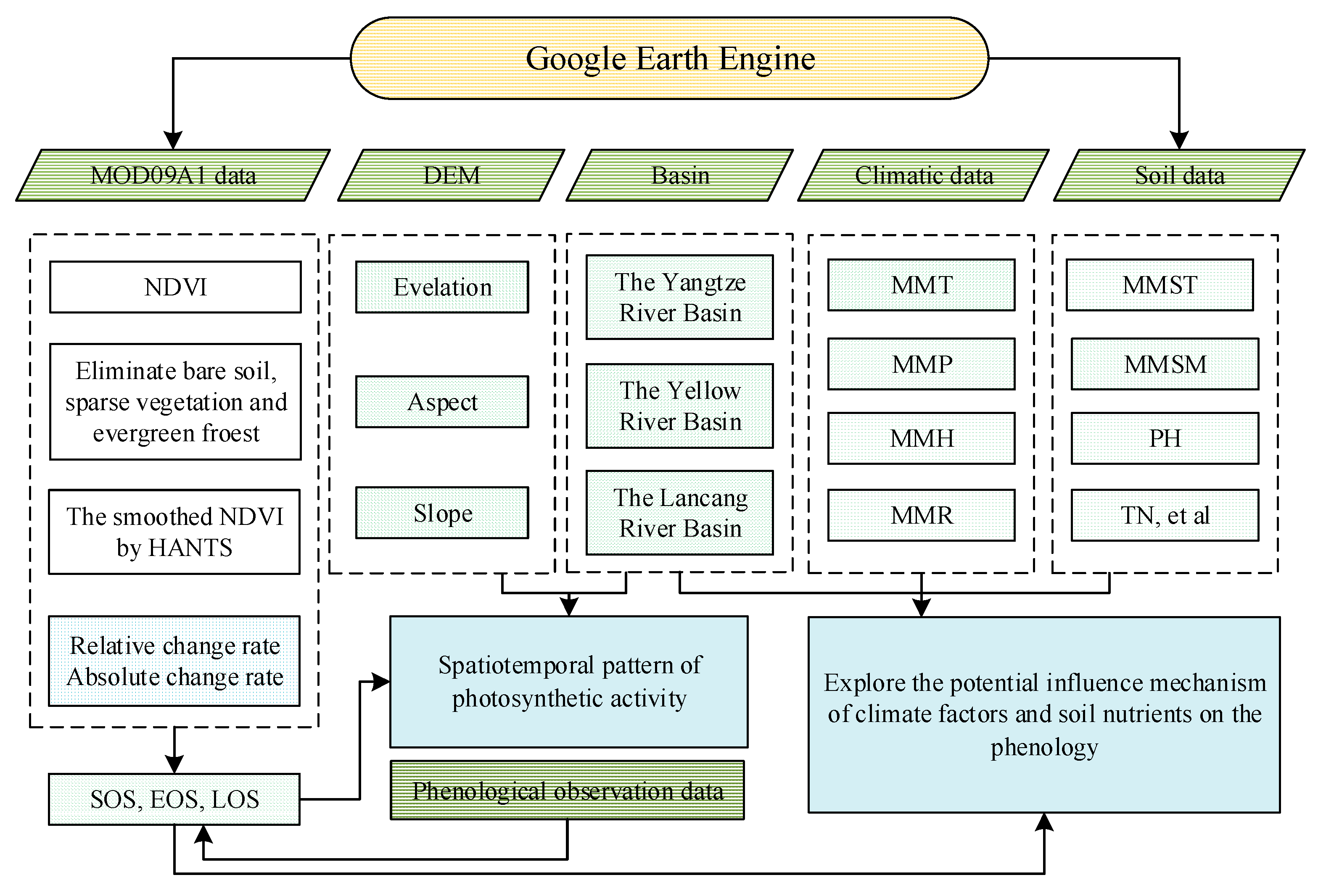
2.1. Processing

The flow chart of research ideas for this paper is as follows (Figure 1). First, we calculated the plant phenology according to the following steps: (1) the NDVI of the TRHR was calculated from MOD09A1 datasets in Google Earth Engine; (2) next, bare soil, sparse vegetation, and evergreen forest pixels were eliminated according to certain requirements; (3) then, the NDVI datasets were smoothed by harmonic analysis of time series (HANTS); (4) we used relative and absolute rates of change to calculate plant phenology (SOS and EOS) based on the NDVI datasets smoothed by HANTS; (5) the phenological data obtained by remote sensing monitoring were verified by using the observation data of phenological stations. Then, we analyzed the spatiotemporal dynamic pattern of plant phenology on different types of terrain and basins. Finally, we explored the potential influence mechanism of climate and soil factors on the phenology of the TRHR based on the structural equation model (SEM) and Pearson correlation coefficients.

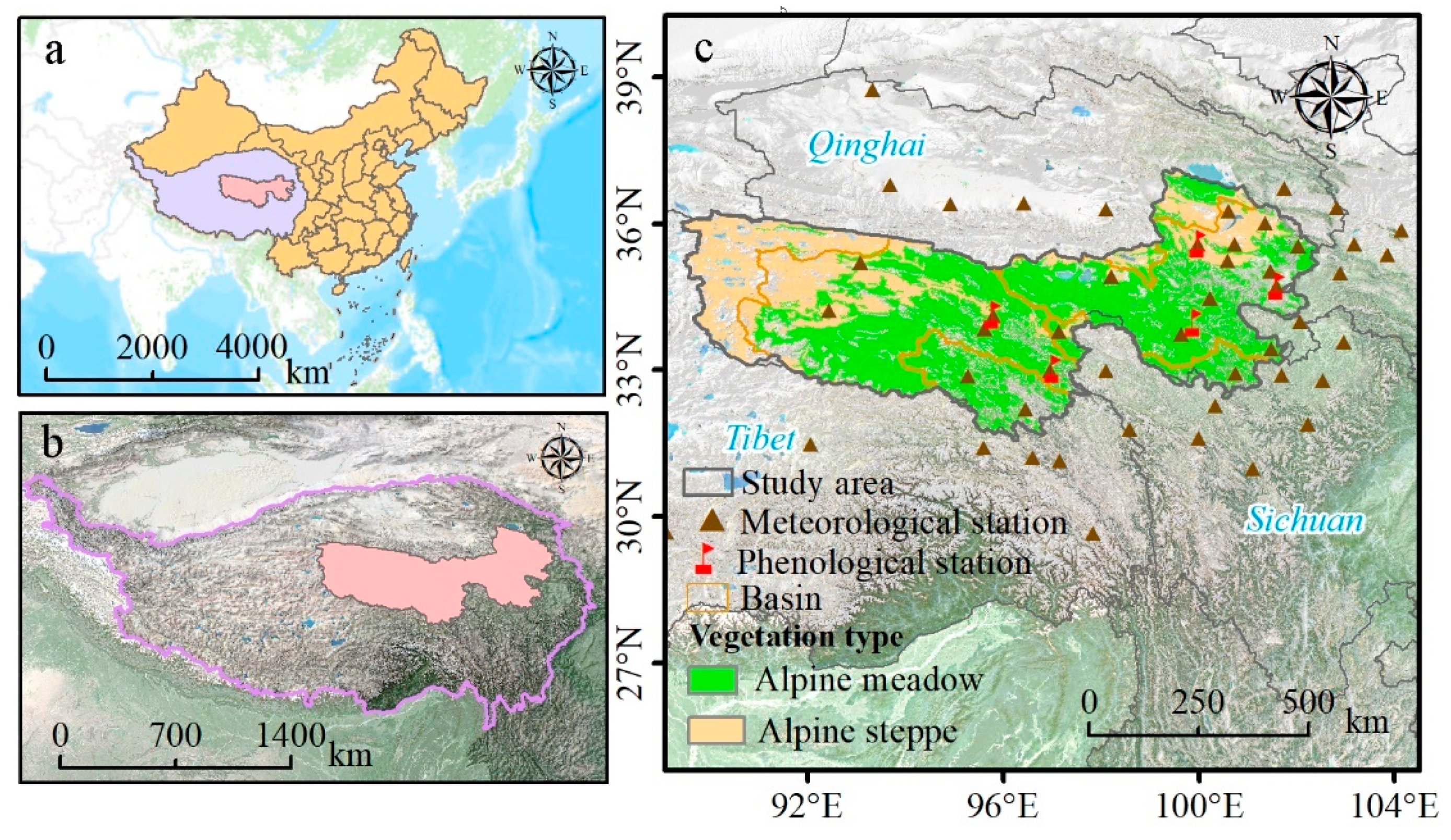
2.2. Study Area

The TRHR (31°39′N–37°10′N, 89°24′E–102°27′E) is located in the hinterland of the Tibetan Plateau and in southern Qinghai Province of China (Figure 2). As the source area for the Yellow, Lancang, and Yangtze rivers, the TRHR supplies approximately 40 billion m³ of water downstream every year. It serves as an important source of freshwater resources in China and Asia and is often referred to as the “Chinese water tower” [26]. The TRHR spans 22 counties and covers an area of about 3.95 × 10⁵ km², and the elevation increases from 1987.5 m in the southeast to 6714.5 m in the northwest, with an average elevation over 4000 m. In 2010, the main land-use types in the TRHR were grassland (68.4%), desert (16.0%), wetland (9.4%), shrub (4.6%), and forest (0.3%), where alpine steppe and alpine meadow were the main types of grassland [27]. The TRHR has major extensive wetlands in China, with abundant lake, river, glacier, and mountain snow resources, and supports the largest alpine wetland ecosystem in the world. Moreover, the TRHR is an important ecological functional zone, a typical ecologically fragile area in China, and is quite sensitive to climate change.

The TRHR experiences a typical plateau continental climate with large daily temperature differences, small annual temperature differences, intense radiation, and a large number of sunshine hours [28]. The TRHR has cool and dry winters with wet and warm summers, mainly caused by the influence of the Asian monsoon and high elevation [29]. Meanwhile, the annual average precipitation in the THRH gradually increased from northwest (262.2 mm) to southeast (772.8 mm), primarily concentrated between June and September owing to the influence of the warm and humid air currents in the southern Bay of Bengal [28,30]. Furthermore, the annual average temperature, sunshine hours, and evaporation of TRHR ranging −5.6 to 7.8 °C, 2300 to 2900 h, and 730–1700 mm, respectively [14,26].

2.3. Data Sources

2.3.1. MOD09A1 Data

The main vegetation types in the TRHR are alpine steppe and alpine meadow. These do not have high amounts of vegetation coverage, with the highest values of NDVI being less than 0.6. Therefore, there are no areas where vegetation is so saturated that the NDVI cannot be accurately expressed. Hence, NDVI was selected in this paper for use in analyzing plant phenological characteristics. Based on a previous study, this paper selected MOD09A1 data products because they have a high temporal resolution, which can provide us with better detailed information related to vegetation growth. The NDVI time-series data came from the Google Earth Engine (https://developers.google.com/earth-engine/datasets/catalog/MODIS_006_MOD09A1 (accessed on 20 July 2020)), with a temporal resolution of 8 days and a spatial resolution of 500 × 500 m. In order to improve the calculated phenological results accurately, we used the following rules for data processing. (1) NDVI was calculated based on the MOD09A1 band using Equations (1) and (2). To eliminate the influence of bare soil, sparse vegetation, and evergreen forest, the pixels of NDVI data in this study had to meet the following requirements: (a) the average value of NDVI should be more than 0.2 in April–October; (b) the maximum value of annual NDVI shall exceed 0.30; (c) the annual maximum value shall occur from July to September; and (d) the average value of NDVI in winter shall be less than 0.4. (3) The NDVI data with a temporal resolution of 1 day was obtained by using HANTS to fit the data, which were processed in steps 1 and 2 (Figure 3a).

2.3.2. Phenological Observation Data

Vegetation phenological observation data (2001–2013) of the THRH used in this study were extracted from the ten-day datasets on crop growth and farmland soil moisture in China, which were obtained from the Chinese Meteorological Administration (http://data.cma.cn/ (accessed on 12 October 2020)). We selected the phenological stations according to the principle that the vegetation type around each station is grassland. Finally, we selected five phenological observation stations (Figure 2c).

2.3.3. Climate Datasets

The meteorological data were selected from the monthly cumulative precipitation, monthly mean relative humidity, and monthly mean air temperature from April to October during 2001 to 2018 for 51 nationally standard meteorological stations in and near the TRHR (Figure 2c), which were provided by the Chinese Meteorological Administration (http://data.cma.cn/ (accessed on 5 July 2020)). Some observational data were missing and had non-uniformity characteristics owing to the influence of changes in meteorological stations and in instruments used to observe. Thus, the regression equation of time series and the homogeneity test of variance were used to fill in the missing values and test for data homogeneity at first in this paper. The commonly used spatial interpolation methods include inverse distance weighted, co-kriging, and thin plate splines (TPS). After comparative experiments, the monthly accumulated precipitation and monthly mean relative humidity were interpolated by the co-kriging method in ArcGIS10.5 software (ESRI, Redlands, CA, USA), with 500 × 500 m resolution. Furthermore, the TPS method of Anusplin software (Centre for Resource and Environmental Studies, Australian National University, Canberra, Australia) was adopted to interpolate the monthly mean temperature at a resolution of 500 × 500 m.

In this study, time-series shortwave radiation data were acquired from the European Centre for Medium-Range Weather Forecasts website (https://cds.climate.copernicus.eu/cdsa-pp#!/dataset/reanalysis-era5-land-monthly-means?tab=overview (accessed on 5 July 2020)), with a temporal resolution of one month and a spatial resolution of 0.1° × 0.1°.

2.3.4. Soil Characteristics Database

In order to explore the influence of soil physical and chemical attributes on plant phenology, we used a database of soil characteristics that was produced by the Land–Atmosphere Interaction Research Group at Sun Yat-sen University (http://globalchange.bnu.edu.cn/home (accessed on 25 October 2020)). The database included information on total N (g/100 g), total P (g/100 g), total K (g/100 k), soil organic matter (g/100 g), alkali-hydrolysable N (mg/kg), available P (mg/kg), available K (mg/kg), cation exchange capacity (me/100 g), porosity (cm³/100 cm³), bulk density (g/cm³), and pH (H₂O). Furthermore, soil moisture and soil temperature data were obtained from Google Earth Engine (https://developers.google.com/earth-engine/datasets/catalog/NASA_FLDAS_NOAH01_C_GL_M_V001#bands (accessed on 25 October 2020)) with a spatial resolution of 0.1° × 0.1° and temporal resolution of one month.

2.3.5. Digital Elevation Model

Digital Elevation Model (DEM) data were collected from the Advanced Spaceborne Thermal Emission and Reflection Radiometer Global Digital Elevation Model (ASTER GDEM) Version 3, which was provided by the US National Aeronautics and Space Administration’s Earth Data website (https://earthdata.nasa.gov/ (accessed on 30 October 2020)), with a spatial resolution of 30 m. For this study, the DEM data were processed with ArcGIS 10.5 to obtain the slope, elevation, and aspect.

2.4. Methods

2.4.1. Extraction of Plant Phenological Information

(1)

NDVI

In this study, on the basis of NDVI that is estimated by the MOD09A1 band information, we calculated the SOS and EOS using the method of the relative and absolute rates of NDVI change, respectively. The NDVI is defined by [31]:

$$NDVI=\left({\rho }_{NIR}-{\rho }_{Red}\right)/\left({\rho }_{NIR}+{\rho }_{Red}\right),$$

(1)

where $\rho$_NIR and $\rho$_Red are the spectral reflectance values calculated in the near-infrared and red bands, respectively.

(2)

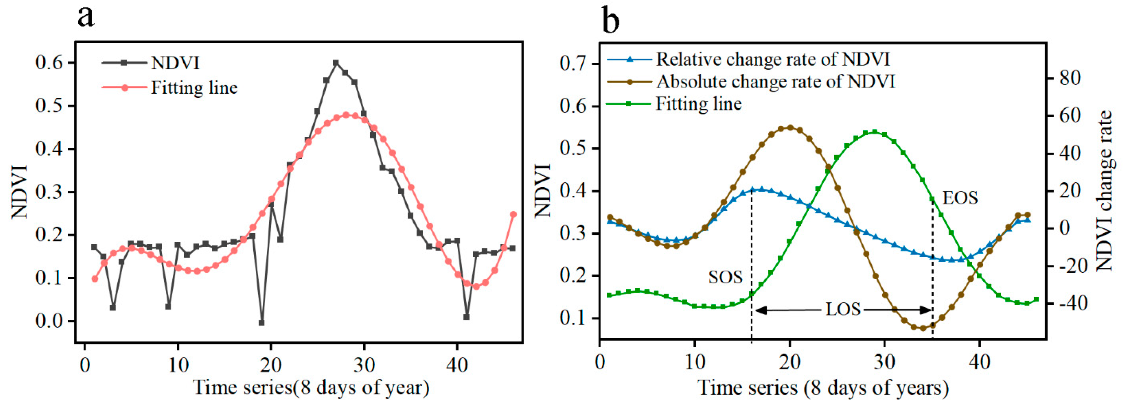
Determination of the SOS and EOS

We used the maximum relative and minimum absolute rates of change in NDVI to calculate the SOS and EOS based on previous studies [14]. The equations of these rates of change can be expressed by:

$${NDVI}_{rate\_rel}=\frac{{NDVI}_{t+1}-{NDVI}_t}{{NDVI}_t}, t\in \left[1,2,\dots ,365\right],$$

(2)

$${NDVI}_{rate\_abs}={NDVI}_{t+1}-{NDVI}_t, t\in \left[1,2,\dots ,365\right],$$

(3)

where NDVI_{rate_rel} and NDVI_{rate_abs} are the relative and absolute rates of change, respectively.

The specific calculation process is as follows. First, we calculated the time (T) when the maximum value appears based on the NDVI time-series data. The NDVI curve was divided into a rising (0, T) and a descending (T, 365) stage. Second, based on Equations (2) and (3), the maximum relative and minimum absolute rates of change were calculated by using the NDVI time-series data. Then, the thresholds of SOS and EOS were determined based on the maximum relative and minimum absolute rates of change, respectively. Third, if the NDVI value was greater than the SOS threshold at time 0 to T, the corresponding date of the year was regarded as the SOS. Similarly, if the NDVI value of some pixels was less than the EOS threshold at time T to 365, the corresponding day of the year plus one was regarded as the EOS (Figure 3b).

2.4.2. The Spatiotemporal Pattern of Plant Phenology

(1)

Linear Regression Analysis

We adopted a linear regression analysis to analyze the monotonic trend of the vegetation phenology and indicators [32,33]. The trend slope in a multi-year regression equation represents the amount of inter-annual change and can be found using the least squares method as follows:

$$Slope=\frac{n·{{\displaystyle \sum }}_{t=1}^{n}t·X_t-{{\displaystyle \sum }}_{t=1}^{n}t{{\displaystyle \sum }}_{t=1}^n{X}_t}{n·{{\displaystyle \sum }}_{t=1}^n{t}^2-{\left({{\displaystyle \sum }}_{t=1}^{n}t\right)}^2},$$

(4)

where Slope refers to the inter-annual trend, n is the number of years of the study, and the X_t is the value of this variable in the t-th year. When the slope is positive or negative, this indicates an increasing or decreasing trend, respectively.

(2)

Standard Deviation Analysis

Standard deviation is a measure of the degree of data dispersion that can reflect the stability or fluctuation of variables [34]. For this study, the stability or fluctuation of plant phenology was calculated by standard deviation based on the pixel scale. The calculation formula is as follows:

$$S_i=\sqrt{\frac{1}{n}{\displaystyle {{\displaystyle \sum }}_{i=1}^n}{\left(X_i-\overline{X}\right)}^2},$$

(5)

where S_i indicates the standard deviation of an X dataset. When the S_i value is larger, the distribution of the data is more discrete and has a larger range of fluctuation. In contrast, when the S_i value is smaller, the distribution of the data is more concentrated and the range of fluctuation is smaller.

2.4.3. Driving Force Analysis

(1)

Pearson Correlation Coefficient

For this paper, we used correlation analysis to determine the relationship between the plant phenology (SOS, EOS, and LOS) and other factors. A higher value indicates a stronger correlation; otherwise, it means a weaker correlation [28,35]. The relevant formula is as follows:

$$R_{xy}=\frac{{{\displaystyle \sum }}_{i=1}^n[[x_i-\overline{x}]·[y_i-\overline{y}]]}{\sqrt{{{\displaystyle \sum }}_{i=1}^n[{[x_i-\overline{x}]}^2·{[y_i-\overline{y}]}^2]}},$$

(6)

where R_xy is the correlation coefficient between x and y, n is the number of years during the study, x_i and y_i are the two sets of variables, and $\overline{x}$ and $\overline{y}$ are the mean values of variables.

(2)

Structural Equation Model

SEM is a method used to analyze the relationship between variables based on a covariance matrix of variables, which includes maximum likelihood, synthesis of factor, and path analyses [24]. It pre-sets the dependence relationship between the factors in the system based on the researcher’s prior knowledge, which can judge the strength of the relationship between the factors and can fit and judge the overall model. In addition, SEM has several advantages. For example, the direct or indirect effects of a particular variable on another variable can be partitioned by SEM, and SEM estimates and reports the total path coefficient to present the strengths of these multiple effects [36]. Since the change in SOS and EOS eventually lead to the change in LOS, this paper only used SEM to explore the potential influence mechanism of climate and soil factors on LOS in the TRHR.

3. Results

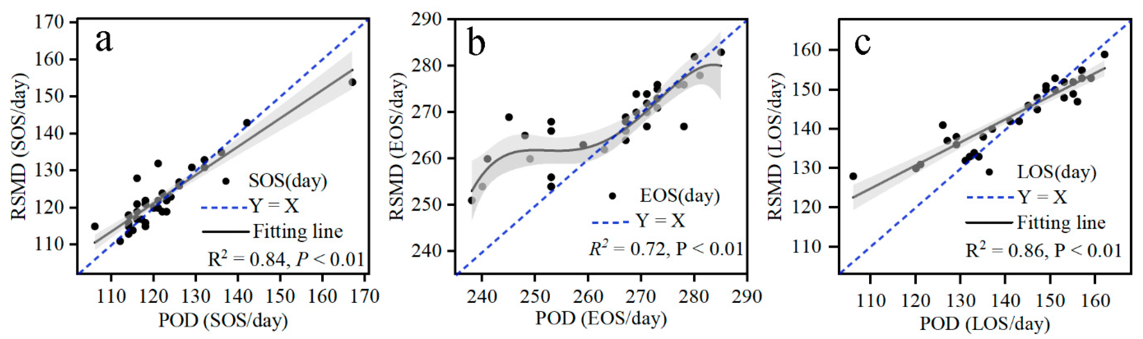
3.1. The Verification of Vegetation Phenological Results

For this study, a regional plant phenological dataset was developed based on data acquired from 2001 to 2018. Figure 4 shows that the remote sensing monitoring data of SOS (R² = 0.84, p < 0.01), EOS (R² = 0.72, p < 0.01), and LOS (R² = 0.86, p < 0.01) have strong similarity with the phenological observation data. Specifically, the times of SOS monitored by remote sensing and observed by phenological stations are distributed near a straight line (Y = X). However, the times of EOS and LOS observed by remote sensing and phenological stations are generally distributed above the straight line (Y = X). This showed that the time product of SOS is highly consistent with the values observed at phenological stations, but the time product of EOS is delayed when compared with that of phenological stations; in addition, the LOS product of remote sensing monitoring is longer than observed at the phenological station (Figure 4).

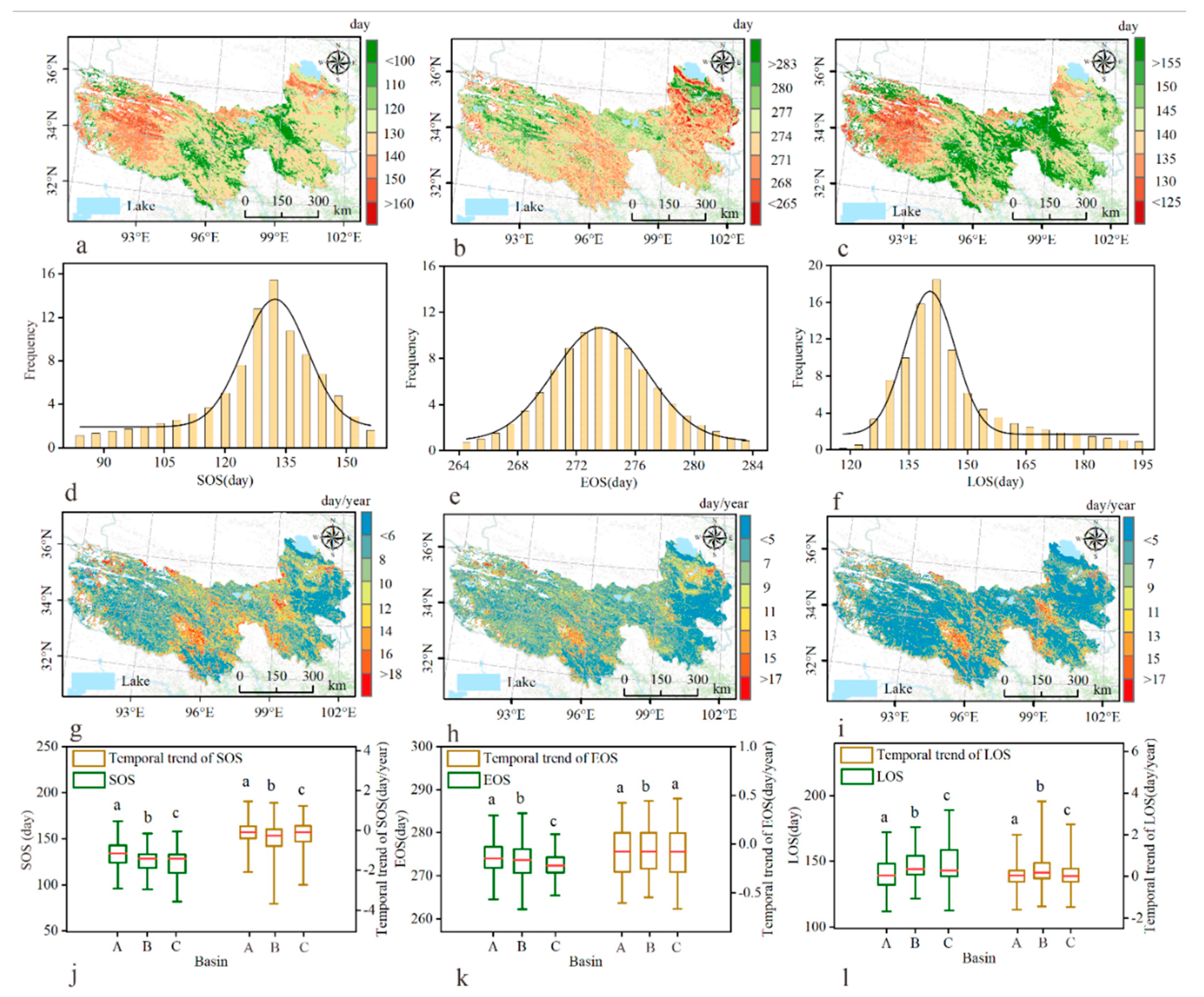
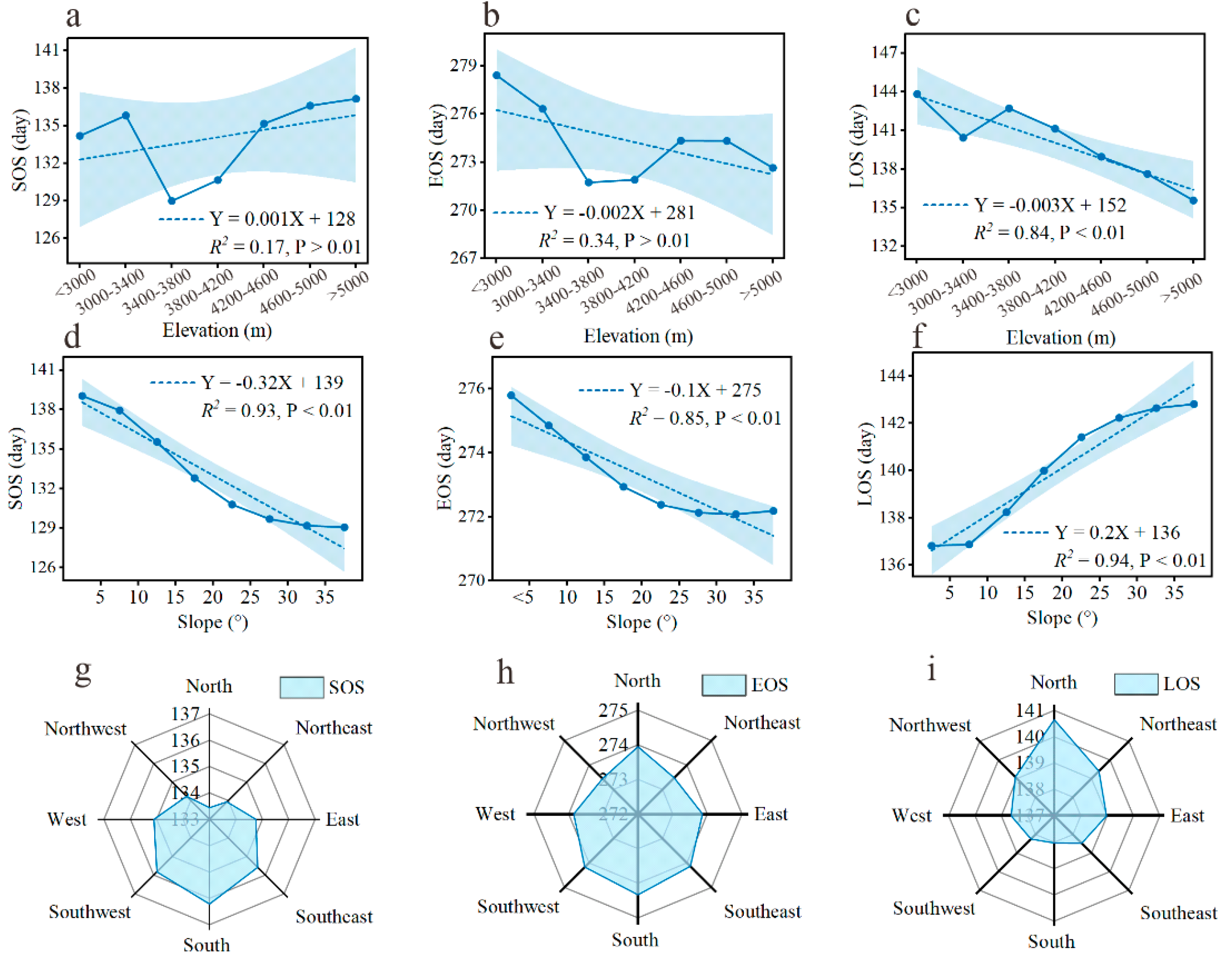
3.2. Spatiotemporal Pattern of Plant Phenology

During the study period, the spatiotemporal trends and standard deviations of SOS, EOS, and LOS had a heterogeneous geographical distribution from 2001 to 2018. The spatial distribution of the multiyear mean SOS primarily occurred between day 100 and 150, and the multiyear average SOS arrived before day 100 in the low-elevation river valley areas of the Yellow and Lancang river basins and appeared after day 150 in some high-elevation or high-latitude areas of the Yangtze River Basin (Figure 5a,d). Similarly, the high value (>16 day/year) of standard deviation for SOS principally occurred in the Lancang River Basin and the southwestern part of the Yangtze River Basin, with the lowest value (<8 day/year) in the center of the Yangtze River Basin and the southeastern part of the Yellow River Basin (Figure 5g). We also found that the Yellow River Basin had the earliest SOS, and the time is in advance (Figure 5j). Furthermore, the spatial distribution of the multiyear average EOS was mainly observed from day 265 to 283, the multiyear average EOS arrived before day 265 in the northeast of the Yellow River Basin, and appeared after day 280 in the center of the Yangtze River Basin (Figure 5b,e). The high value of the standard deviation of EOS was mainly in the Yangtze and Lancang river basins (Figure 5h). In addition, we also compared the temporal trend of EOS in different basins; the earliest EOS was in the Lancang River Basin and the latest in the Yangtze River Basin (Figure 5k). Last, the spatial distribution of the multiyear average LOS was mainly between day 120 and 160, while the multiyear average LOS was longer than day 150 in some areas of the Yellow and Lancang river basins (Figure 5c,f). The high value of the standard deviation of LOS was mainly distributed in the Lancang and Yangtze river basins (Figure 5i). Furthermore, we also found that the Lancang River Basin had the longest LOS, which is becoming longer over time (Figure 5l).

For this study, SOS, EOS, and LOS have different distributions at different elevations, slopes, and aspects in the THRH (Figure 6). Specifically, the SOS generally showed an upwards (0.001 day/m, R² = 0.17, p > 0.01) trend with an increase in elevation (Figure 6a). This phenomenon indicates that with an increase in elevation, the SOS is delayed. In contrast, EOS and LOS decreased (0.002 day/m, R² = 0.34, p > 0.01 and 0.003 day/m, R² = 0.84, p < 0.01, respectively) as elevation increased, which represents that the time of EOS and the LOS advance and shorten with an increase in elevation, respectively (Figure 6b–c). Furthermore, SOS and EOS decreased significantly (0.32 day/°, R² = 0.93, p < 0.01 and 1 day/°, R² = 0.85, p < 0.01, respectively) with an increase in slope (Figure 6d–e). This indicates that the time of SOS and EOS advance with an increase in slope. However, the relationship between LOS and slope was the opposite of that between SOS or EOS and slope. The LOS was prolonged (0.2 day/°, R² = 0.94, p < 0.01) with an increase in slope (Figure 6f). Last, we find the north-facing slopes had the lowest value of SOS but had the highest value of EOS and LOS. The results showed that the times of SOS, EOS, and LOS were the earliest, latest, and longest, respectively, on the north slope.

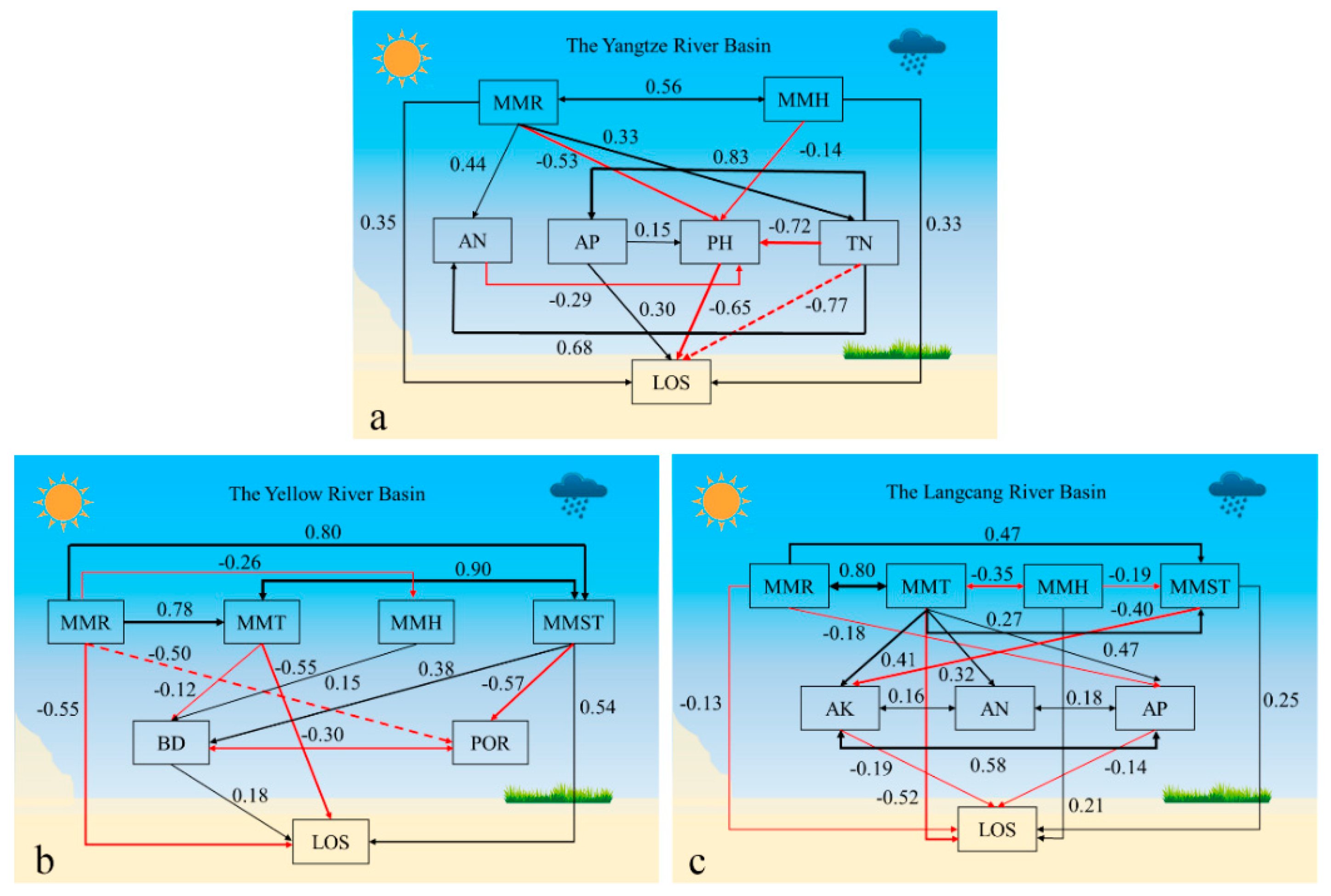
3.3. Linking Climatic and Soil Factors to Plant Phenology

The correlation coefficients between plant phenology connected to the principal climate characteristics along with soil physical and chemical factors were significant at p < 0.01 (

Table 1. The relationships between plant phenology and the principal climate factors along with soil physical and chemical factors at different stages (SOS, EOS, and LOS) in the Yangtze River Basin, Yellow River Basin, and Lancang River Basin.

	MMST	MMH	MMT	MMP	MMSM	AN	AP	TN	SOM	CEC	TP	AK	POR	MMR	PH	TK	BD
SOS a	−0.06 **	−0.38 **	−0.13 **	−0.68 **	−0.37 **	−0.39 **	−0.31 **	−0.24 **	−0.22 **	−0.23 **	0.04 **	0.09 **	−0.03 *	0.73 **	0.50 **	0.44 **	0.06 **
SOS b	0.48 **	−0.16 **	0.50 **	−0.04 **	0.31 **	−0.04 **	0.10 **	0.09 **	0.09 **	0.12 **	0.14 **	0.15 **	−0.19 **	0.50 **	0.09 **	0.10 **	−0.05 **
SOS c	0.55 **	−0.36 **	0.65 **	0	0.43 **	0.31 **	0.35 **	0.29 **	0.23 **	0.26 **	0.05	0.50 **	−0.26 **	0.53 **	−0.09 **	0.12 **	−0.08 **
EOS a	0.22 **	−0.16 **	0.10 **	−0.45 **	−0.27 **	−0.27 **	−0.17 **	−0.17 **	−0.16 **	−0.19 **	0.08 **	0.05 **	0.02	0.44 **	0.40 **	0.41 **	0.02
EOS b	0.24 **	−0.23 **	0.20 **	−0.23 **	−0.39 **	−0.32 **	0	−0.12 **	−0.07 **	−0.07 **	0.05 **	0.04 **	−0.21 **	0.03	0.37 **	0.01	−0.06 **
EOS c	−0.41 **	0.08 **	−0.43 **	−0.33 **	−0.22 **	−0.12 **	0.13 **	0.01	0.04	0.04	0.09 **	−0.12 **	0.24 **	−0.36 **	0.07 **	−0.26 **	−0.18 **
LOS a	0.17 **	0.52 **	0.21 **	0.21 **	−0.02	0.38 **	0.33 **	0.24 **	0.21 **	0.21 **	−0.01	−0.09 **	0.06 **	0.53 **	−0.46 **	−0.37 **	−0.07 **
LOS b	−0.43 **	0.10 **	−0.46 **	0.02	−0.02	−0.05 **	−0.10 **	−0.13 **	−0.11 **	−0.14 **	−0.13 **	−0.15 **	0.14 **	−0.55 **	0.01	−0.10 **	0.04 **
LOS c	−0.65 **	0.41 **	−0.69 **	−0.08 **	−0.16 **	−0.32 **	−0.33 **	−0.28 **	−0.22 **	−0.25 **	−0.03	−0.50 **	0.28 **	−0.58 **	0.10 **	−0.15 **	0.06 *

MMR, MMP, MMT, MMH, MMSM, and MMST indicate monthly mean shortwave radiation, precipitation, temperature, relative humidity, soil moisture, and soil temperature, respectively. AK, AN, AP, BD, CEC, pH, POR, SOM, TK, TN, and TP represent available K, alkali-hydrolysable N, available P, bulk density, cation exchange capacity, pH (H₂O), porosity, soil organic matter, total K, total N, and total P, respectively. ** and * indicate significance coefficients of less than p < 0.01 and p < 0.05, respectively. ^a,b and ^c represent the Yangtze River Basin, Yellow River Basin, and Lancang River Basin, respectively.

). In the Yangtze River Basin, our results show that the SOS was positively correlated with monthly mean shortwave radiation (MMR; 0.73**), pH (0.50**), and total phosphorus (TK) (0.44**) but negatively correlated with monthly mean precipitation (MMP; −0.68**), available nitrogen (AN; −0.39**), monthly mean relative humidity (MMH; −0.38**), and monthly mean soil moisture (MMSM; −0.37**). Furthermore, the correlation coefficients between EOS and MMP, pH, TK, and MMR were −0.45**, 0.40**, 0.41**, and 0.44**. Finally, we found that LOS was significantly negatively correlated with pH (−0.46**) and TK (−0.37**), but LOS was significantly positively correlated with MMR (0.53**), MMH (0.52**), and AN (0.38**) during the growing season.

In the Yellow River Basin, significant positive relationships were observed between SOS and monthly mean temperature (MMT; 0.50**), monthly mean soil temperature (MMST; 0.48**), MMR (0.50**), and MMSM (0.31**). However, the EOS was significantly negatively correlated with MMSM (−0.39**) and AN (−0.32**) and significantly positively correlated with pH (0.37**). In addition, we found that LOS was significantly negatively correlated with MMR (−0.55**), MMT (−0.46**), and MMST (−0.43**).

In the Lancang River Basin, the results indicated that there were significant positive correlations between the SOS and AK (0.50**), MMT (0.65**), MMST (0.55**), MMR (0.53**), and MMSM (0.43**). In addition, we found that the EOS was significantly negatively correlated with MMST (−0.41**), MMT (−0.43**), MMR (−0.36**), and MMP (−0.33**). Meanwhile, we also found that the correlation coefficients between LOS and MMH, MMT, MMST, MMR, and AK were 0.41**, −0.69**, −0.65**, −0.58**, and −0.50** (Table 1).

The mechanisms involved in patterns in the length of the plant growing season in different basins were explored using SEM. In general, the effect of soil factors on LOS is greater than that of climate factors in the Yangtze River Basin. Specifically, AP, pH, and TN had a significant effect on the LOS (p < 0.01), with scores of 0.30, −0.65, and −0.77, respectively. However, the impact scores of MMR and MMH on LOS were only 0.35 and 0.33 (Figure 7a). Path analyses identified that climate factors, as a key functional indicator of the LOS in the Yellow River Basin, had either direct or indirect effects via edaphic factors. Specifically, the MMR (scored at −0.55), MMT (scored at −0.30), and MMST (scored at 0.54) had significant effects on the LOS (Figure 7b). Furthermore, in the Lancang River Basin, the effects of each variable on LOS were different (ranging from −0.52 to 0.25), which suggests that the LOS might be co-determined by both the soil and climatic factors (Figure 7c). This assumption was confirmed in that soil factors were significantly affected by climatic factors. Specifically, the AK (scored at 0.41), AP (scored at 0.27), and AN (scored at 0.32) were significantly (p < 0.01) influenced by MMT. Furthermore, AK and AP had a significant interaction (scored at 0.58).

4. Discussion

4.1. Spatial–Temporal Patterns of Plant Phenology

The time of the SOS experienced a significant downtrend (slope < 0), but the LOS increased over time (slope > 0) during 2001–2018 in the Yellow River Basin (Figure 5j,l). The research showed that with the increase of annual mean precipitation, temperature, relative humidity, shortwave radiation, soil temperature, and soil moisture in the Yellow River Basin during the SOS and LOS period, the time of SOS and LOS became earlier and longer (Figures S3 and S5). The favorable water and heat environment provided important resources for vegetative growth [37,38]. Water supply determines whether the photosynthesis occurs normally with an adequate CO₂ concentration and sufficient light [24,39]. Meanwhile, water is also an indispensable intermediary used to ensure nutrient substance transport [24,40]. Therefore, the increased humidity, precipitation, and soil moisture played a crucial role in the advance of the timing of the SOS and the prolonged nature of the LOS. In addition to water, temperature is also an indispensable factor in vegetative growth. An increase in temperature could facilitate vegetative growth if plants do not encounter water limitation [4,40]. Furthermore, climate warming can stimulate the enzymatic activities involved in photosynthesis [24,41], accelerate the mineralization and decomposition of organic matter [42], and extend the length of the vegetative growing season [7,43]. In general, the improvement of water and heat conditions visibly promoted the growth of vegetation in the TRHR.

The multi-year (2001–2018) average time of the SOS, EOS, and LOS in the TRHR presented a discrepant geographical pattern. In general, the time of the plant SOS was earliest in the Lancang and western Yellow river basins, while the time of the plant EOS was latest in the middle of the Yangtze River Basin. The duration of the vegetation growing season was longest in the Lancang and western Yellow river basins (Figure 5a–c). This phenomenon is closely related to the distribution of climate in the TRHR. The TRHR’s climate is dominated by the East Asian monsoon, because the Himalayan Mountain Range obstructs the Indian monsoon [44,45] and causes a gradual reduction in precipitation, relative humidity, and soil moisture from southeast to northwest (Figures S2–S5). Likewise, vegetative growth is easily affected by climate change in the TRHR as also supported by previous studies [46,47]. Furthermore, the time of the plant SOS was delayed with an increase in elevation, but the times of the EOS or LOS were advanced or shortened, respectively, with an increase in elevation (Figure 6a–c). Possible reasons include the following: the ecosystems of high elevation areas are fragile, and the vegetative growth is vulnerable to extreme weather, such as extreme low temperature and frost. Another possibility is that the perennial snowfall occurring in high elevation regions causes low temperatures, which weaken the activity of soil microorganisms [14]. In contrast, with an increase in slope, the time of the SOS and EOS are in advance, while the LOS is prolonged (Figure 6d–f). The main reason for this result is that the areas with high slopes were mainly concentrated in the Lancang and the south part of the Yellow river basins, which have lower elevations (Figure S1). This provides reliable water and temperatures to guarantee the normal operation of vegetative photosynthesis. Finally, the vegetation of shady slopes started growing earlier in the growing season, ended later, and so had the longest growing season (Figure 6g–i), mainly due to the strong illumination and high temperature that accelerated soil organic matter mineralization and caused sunny slopes to have less soil moisture [48]. However, the shady slopes have soft solar radiation, moist soil, less moisture evaporation, and higher soil fertility [49,50].

4.2. The Response of the Plant Phenology to Climate Change

Our results illustrate that the variations in soil resources (e.g., pH and soil total N) that support vegetative growth, together with the climatic conditions that were suitable for vegetative growth, co-explained the phenological differences in plants from different basins. Specifically, the Yangtze River Basin is affected by the East Asian monsoon and elevation (Figure S1a), insufficient water supply, and relatively low temperatures, and low levels of soil nutrients constrained the growth of vegetation at the start of the growing season (Figures S2–S3). The air and soil temperatures are relatively low with less precipitation and soil moisture from April to May, which is not enough to support the transport of nutrients in plants, soil nutrient absorption by roots, and photosynthesis [24,51]. With the increased temperature, winter snow, permafrost, and glaciers have begun to melt slowly, and mineralization and decomposition of organic matter are accelerated [52,53] so that warmer temperatures provide plants with earlier opportunities to germinate [32]. However, the Yellow and Lancang river basins have higher temperatures and more shortwave radiation and precipitation than other areas owing to the lower elevation (Figures S1–S5). The increase in precipitation significantly increased soil carbon and N content, making it easier for plants to absorb nutrients owing to an increase in leaf stomatal conductance and photosynthesis [24,54]. This may explain why temperature is more important for seed germination than water at the start of the growing season in the Yangtze River Basin, while water and heat are equally important for seed germination in the Yellow and Lancang river basins. In addition, the Yangtze River Basin lies in a high elevation area, which has thin air, strong solar radiation, and a long sunshine season (Figure S3). At high elevations, the decomposition of soil litter slows, which promotes the accumulation of organic matter due to the low temperatures caused by snow cover, which, in turn, slows the activity of soil microorganisms [14]. Thus, the growing season ends relatively late in the Yangtze River Basin. An interesting question arises: why were the soil factors having a greater impact on LOS in the Yangtze River Basin when compared with the Yellow and Lancang river basins (Table 1 and Figure 7)? Here, we propose one explanation. The precipitation, air temperature, relative humidity, soil moisture, and soil temperature showed a decreasing trend from southeast (the Yellow River Basin) to northwest (the Yangtze River Basin) in the TRHR because of the influence of the monsoon and elevation (Figures S2–S5). This situation led to low air temperature and less precipitation in the Yangtze River Basin, which does not provide enough energy for the growth of plants. At this time, the melting of permafrost and glaciers and the mineralization of soil organic matter provide energy for plant growth. However, the Yellow and the Lancang river basins have high air temperature, soil temperature, precipitation, and soil moisture, which can provide sufficient energy for plant growth.

4.3. Limitations of the Current Study

Despite the achievements in this study, large uncertainties still exist. In addition to NDVI, multiple vegetation indices can be used to reflect vegetation dynamics, such as EVI and LAI [1,34]. Note that the calculated plant phenology results may be vary based on the differences in resolution and quality of datasets using different vegetation indices. Furthermore, the present smoothing methods of remote sensing time series data have great differences in the model structure, which may result in great differences among the extracted plant phenology results [55,56]. Meanwhile, although the smoothing method used for the remote sensing time series is the same, different smoothing parameters also cause different results. Although the guidelines for some smoothing methods suggested using default parameter values when they were proposed, the best parameter values may vary because of the different growth trajectories of vegetation at specific sites, which lead to a difference in plant phenology in various regions and with different vegetation types [57,58]. Moreover, many methods can be used to extract plant phenological information, and they all have a certain level of applicability. Therefore, different methods may lead to different conclusions regarding the same question [56]. As mentioned above, it is necessary to further check whether the plant phenological results calculated from different datasets, smoothing methods of remote sensing time series, smoothing parameters, and phenology extraction methods provide the same or similar results and to improve the credibility of the results. Furthermore, there are many factors that affect plant phenology. Some changes in phenology are caused by climatic and soil factors; other decisive factors have shown effects on plant phenology, such as flash floods and extreme drought. Hence, more attention should be paid to the relationship between plant phenology and natural disasters in future studies.

5. Conclusions

In the present study, we calculated plant phenology information in the TRHR based on the MOD09A1 dataset using the method of HANTS and the relative and absolute rates of change on Google Earth Engine. Meanwhile, the extracted plant phenology results were verified using plant phenology station data. Then, we explored the spatiotemporal patterns of plant phenology based on linear regression and standard deviation analyses. Finally, the potential influence mechanism of climatic and soil factors on phenology was analyzed using Pearson correlation coefficients and an SEM model. The verification of plant phenological results shows that our results were well-correlated with observational data acquired by phenological stations; the determination coefficients of SOS, EOS, and LOS stages were 0.84, 0.72, and 0.86, respectively. The temporal variation of the SOS and LOS indicated that the SOS advanced while the LOS extended. As for spatial patterns, the SOS was the earliest and the LOS was the longest in the Lancang River Basin, while the EOS was the latest in the Yangtze River Basin. Furthermore, the spatial distributions of SOS, EOS, and LOS have strong spatial heterogeneity at different elevations, slopes, and aspects. The potential influence mechanism of climatic and soil factors on the phenology indicated that plant phenology in the Yangtze River Basin is mainly affected by soil factors, while that in the Yellow and Lancang river basins is mainly impacted by climatic factors. The results of this study revealed the spatiotemporal patterns of plant phenology of the TRHR and emphasize the important role of soil factors, precipitation, and temperature in controlling plant phenological dynamics. These findings might help to reveal the mechanisms of potential impacts on plant phenology in alpine wetland ecosystems and provide a theoretical basis for ecosystem management.

References

- O’Neill, B.C.; Oppenheimer, M.; Warren, R.; Hallegatte, S.; Kopp, R.E.; Pörtner, H.O.; Scholes, R.; Birkmann, J.; Foden, W.; Licker, R.; et al. IPCC reasons for concern regarding climate change risks. Nat. Clim. Chang. 2017, 7, 28–37. [Google Scholar] [CrossRef] [Green Version]
- Zhang, G.; Zhang, Y.; Dong, J.; Xiao, X. Green-up dates in the Tibetan Plateau have continuously advanced from 1982 to 2011. Proc. Natl. Acad. Sci. USA 2013, 110, 4309–4314. [Google Scholar] [CrossRef] [Green Version]
- Brandt, L.A.; Butler, P.R.; Handler, S.D.; Janowiak, M.K.; Shannon, P.D.; Swanston, C.W. Integrating science and management to assess forest ecosystem vulnerability to climate change. J. For. 2017, 115, 212–221. [Google Scholar] [CrossRef]
- Piao, S.; Friedlingstein, P.; Ciais, P.; Viovy, N.; Demarty, J. Growing season extension and its impact on terrestrial carbon cycle in the Northern Hemisphere over the past 2 decades. Glob. Biogeochem. Cycles 2007, 21. [Google Scholar] [CrossRef]
- Gusewell, S.; Furrer, R.; Gehrig, R.; Pietragalla, B. Changes in temperature sensitivity of spring phenology with recent climate warming in Switzerland are related to shifts of the preseason. Glob. Chang. Biol. 2017, 23, 5189–5202. [Google Scholar] [CrossRef]
- Richardson, A.D.; Keenan, T.F.; Migliavacca, M.; Ryu, Y.; Sonnentag, O.; Toomey, M. Climate change, phenology, and phenological control of vegetation feedbacks to the climate system. Agric. For. Meteorol. 2013, 169, 156–173. [Google Scholar] [CrossRef]
- Dragoni, D.; Schmid, H.P.; Wayson, C.A.; Potter, H.; Grimmond, C.S.B.; Randolph, J.C. Evidence of increased net ecosystem productivity associated with a longer vegetated season in a deciduous forest in south-central Indiana, USA. Glob. Chang. Biol. 2011, 17, 886–897. [Google Scholar] [CrossRef]
- Geng, X.; Fu, Y.H.; Hao, F.; Zhou, X.; Zhang, X.; Yin, G.; Vitasse, Y.; Piao, S.; Niu, K.; de Boeck, H.J.; et al. Climate warming increases spring phenological differences among temperate trees. Glob. Chang. Biol. 2020, 26, 5979–5987. [Google Scholar] [CrossRef]
- Gao, M.; Wang, X.; Meng, F.; Liu, Q.; Li, X.; Zhang, Y.; Piao, S. Three-dimensional change in temperature sensitivity of northern vegetation phenology. Glob. Chang. Biol. 2020, 26, 5189–5201. [Google Scholar] [CrossRef]
- Shen, X.; An, R.; Feng, L.; Ye, N.; Zhu, L.; Li, M. Vegetation changes in the Three-River Headwaters Region of the Tibetan Plateau of China. Ecol. Indic. 2018, 93, 804–812. [Google Scholar] [CrossRef]
- Zhang, W.; Jin, H.; Shao, H.; Li, A.; Li, S.; Fan, W. Temporal and spatial variations in the leaf area index and its response to topography in the Three-River Source Region, China from 2000 to 2017. ISPRS Int. J. Geo Inf. 2021, 10, 33. [Google Scholar] [CrossRef]
- Binghong, H.; Bingrong, Z.; Henghe, Z.; Mingming, S.; Ying, S.; Decao, N.; Hua, F. Relationships between grassland vegetation turngreen and climate factors in the Three-river Resource region. Acta Ecol. Sin. 2019, 39, 5635–5641. [Google Scholar]
- Qiang, L. Phenology response of vegetation to hydrothermal condition in Three-river Source Region for the last 12 years. Arid Zone Res. 2016, 33, 150–158. [Google Scholar]
- Chen, T.; Yi, G.; Zhang, T.; Wang, Q.; Bie, X. A method for determining vegetation growth process using remote sensing data: A case study in the Three-River Headwaters Region, China. J. Mt. Sci. 2019, 16, 2001–2014. [Google Scholar] [CrossRef]
- Han, H.; Bai, J.; Ma, G.; Yan, J. Vegetation phenological changes in multiple landforms and responses to climate change. ISPRS Int. J. Geo-Inf. 2020, 9, 111. [Google Scholar] [CrossRef] [Green Version]
- Niu, B.; Zhang, X.; Piao, S.; Janssens, I.A.; Fu, G.; He, Y.; Zhang, Y.; Shi, P.; Dai, E.; Yu, C.; et al. Warming homogenizes apparent temperature sensitivity of ecosystem respiration. Sci. Adv. 2021, 7, eabc7358. [Google Scholar] [CrossRef]
- Chen, A.; Huang, L.; Liu, Q.; Piao, S. Optimal temperature of vegetation productivity and its linkage with climate and elevation on the Tibetan Plateau. Glob. Chang. Biol. 2021, 27, 1942–1951. [Google Scholar] [CrossRef]
- Cong, N.; Shen, M.; Yang, W.; Yang, Z.; Zhang, G.; Piao, S. Varying responses of vegetation activity to climate changes on the Tibetan Plateau grassland. Int. J. Biometeorol. 2017, 61, 1433–1444. [Google Scholar] [CrossRef]
- Menzel, A.; Sparks, T.H.; Estrella, N.; Koch, E.; Aasa, A.; Ahas, R.; Alm-Kübler, K.; Bissolli, P.; Braslavská, O.G.; Briede, A.; et al. European phenological response to climate change matches the warming pattern. Glob. Chang. Biol. 2006, 12, 1969–1976. [Google Scholar] [CrossRef]
- Yun, J.; Jeong, S.-J.; Ho, C.-H.; Park, C.-E.; Park, H.; Kim, J. Influence of winter precipitation on spring phenology in boreal forests. Glob. Chang. Biol. 2018, 24, 5176–5187. [Google Scholar] [CrossRef]
- Nemani, R.R.; Keeling, C.D.; Hashimoto, H.; Jolly, W.M.; Piper, S.C.; Tucker, C.J.; Myneni, R.B.; Running, S.W. Climate-driven increases in global terrestrial net primary production from 1982 to 1999. Science 2003, 300, 1560–1563. [Google Scholar] [CrossRef] [Green Version]
- Chapin, F.S., III; Matson, P.A.; Vitousek, P. Principles of Terrestrial Ecosystem Ecology; Springer Science & Business Media: Berlin, Germany, 2002; pp. 369–397. [Google Scholar]
- Yue, K.; Peng, Y.; Peng, C.; Yang, W.; Peng, X.; Wu, F. Stimulation of terrestrial ecosystem carbon storage by nitrogen addition: A meta-analysis. Sci. Rep. 2016, 6. [Google Scholar] [CrossRef] [Green Version]
- Sun, J.; Zhou, T.C.; Liu, M.; Chen, Y.C.; Liu, G.H.; Xu, M.; Shi, P.L.; Peng, F.; Tsunekawa, A.; Liu, Y.; et al. Water and heat availability are drivers of the aboveground plant carbon accumulation rate in alpine grasslands on the Tibetan Plateau. Glob. Ecol. Biogeogr. 2019, 29, 50–64. [Google Scholar] [CrossRef] [Green Version]
- Gower, S.T.; Kucharik, C.J.; Norman, J.M. Direct and indirect estimation of leaf area index, f APAR, and net primary production of terrestrial ecosystems. Remote Sens. Environ. 1999, 70, 29–51. [Google Scholar] [CrossRef]
- Jiang, C.; Zhang, L. Ecosystem change assessment in the Three-river Headwater Region, China: Patterns, causes, and implications. Ecol. Eng. 2016, 93, 24–36. [Google Scholar] [CrossRef]
- Xianfeng, L.; Jinshui, Z.; Xiufang, Z.; Yaozhong, P.; Yanxu, L.; Donghai, Z.; Zhihui, L. Spatiotemporal changes in vegetation coverage and its driving factors in the Three-River Headwaters Region during 2000–2011. J. Geogr. Sci. 2014, 24, 288–302. [Google Scholar]
- Zheng, D.; Wang, Y.; Hao, S.; Xu, W.; Lv, L.; Yu, S. Spatial-temporal variation and tradeoffs/synergies analysis on multiple ecosystem services: A case study in the Three-River Headwaters region of China. Ecol. Indic. 2020, 116, 106494. [Google Scholar] [CrossRef]
- Zheng, Y.; Han, J.; Huang, Y.; Fassnacht, S.R.; Xie, S.; Lv, E.; Chen, M. Vegetation response to climate conditions based on NDVI simulations using stepwise cluster analysis for the Three-River Headwaters region of China. Ecol. Indic. 2018, 92, 18–29. [Google Scholar] [CrossRef]
- Zeng, N.; He, H.; Ren, X.; Zhang, L.; Zeng, Y.; Fan, J.; Li, Y.; Niu, Z.; Zhu, X.; Chang, Q. The utility of fusing multi-sensor data spatio-temporally in estimating grassland aboveground biomass in the three-river headwaters region of China. Int. J. Remote Sens. 2020, 41, 7068–7089. [Google Scholar] [CrossRef]
- Piao, S.; Cui, M.; Chen, A.; Wang, X.; Ciais, P.; Liu, J.; Tang, Y. Altitude and temperature dependence of change in the spring vegetation green-up date from 1982 to 2006 in the Qinghai-Xizang Plateau. Agric. For. Meteorol. 2011, 151, 1599–1608. [Google Scholar] [CrossRef]
- Li, L.; Zhang, Y.; Liu, L.; Wu, J.; Wang, Z.; Li, S.; Zhang, H.; Zu, J.; Ding, M.; Paudel, B. Spatiotemporal patterns of vegetation greenness change and associated climatic and anthropogenic drivers on the Tibetan Plateau during 2000–2015. Remote Sens. 2018, 10, 1525. [Google Scholar] [CrossRef] [Green Version]
- Xu, X.; Liu, H.; Lin, Z.; Jiao, F.; Gong, H. Relationship of abrupt vegetation change to climate change and ecological engineering with multi-timescale analysis in the Karst Region, Southwest China. Remote Sens. 2019, 11, 1564. [Google Scholar] [CrossRef] [Green Version]
- He, D.; Huang, X.; Tian, Q.; Zhang, Z. Changes in vegetation growth dynamics and relations with climate in inner Mongolia under more strict multiple pre-processing (2000–2018). Sustainability 2020, 12, 2534. [Google Scholar] [CrossRef] [Green Version]
- Sun, H.; Wang, J.; Xiong, J.; Bian, J.; Jin, H.; Cheng, W.; Li, A. Vegetation change and its response to climate change in Yunnan Province, China. Adv. Meteorol. 2021, 2021, 8857589. [Google Scholar] [CrossRef]
- Shipley, B. Cause and correlation in biology. Ann. Bot. 2002, 90, 777–778. [Google Scholar]
- Zhang, Y.; Gao, J.; Liu, L.; Wang, Z.; Ding, M.; Yang, X. NDVI-based vegetation changes and their responses to climate change from 1982 to 2011: A case study in the Koshi River Basin in the middle Himalayas. Glob. Planet. Chang. 2013, 108, 139–148. [Google Scholar] [CrossRef]
- Kong, D.; Zhang, Q.; Singh, V.P.; Shi, P. Seasonal vegetation response to climate change in the Northern Hemisphere (1982–2013). Glob. Planet. Chang. 2017, 148, 1–8. [Google Scholar] [CrossRef] [Green Version]
- Ye, C.; Sun, J.; Liu, M.; Xiong, J.; Zong, N.; Hu, J.; Huang, Y.; Duan, X.; Tsunekawa, A. Concurrent and lagged effects of extreme drought induce net reduction in vegetation carbon uptake on Tibetan Plateau. Remote Sens. 2020, 12, 2347. [Google Scholar] [CrossRef]
- Yao, Y.; Wang, X.; Li, Y.; Wang, T.; Shen, M.; Du, M.; He, H.; Li, Y.; Luo, W.; Ma, M.; et al. Spatiotemporal pattern of gross primary productivity and its covariation with climate in China over the last thirty years. Glob. Chang. Biol. 2018, 24, 184–196. [Google Scholar] [CrossRef]
- Davidson, E.A.; Janssens, I.A. Temperature sensitivity of soil carbon decomposition and feedbacks to climate change. Nature 2006, 440, 165–173. [Google Scholar] [CrossRef]
- Kim, D.G.; Vargas, R.; Bond-Lamberty, B.; Turetsky, M.R. Effects of soil rewetting and thawing on soil gas fluxes: A review of current literature and suggestions for future research. Biogeosciences 2012, 9, 2459–2483. [Google Scholar] [CrossRef] [Green Version]
- Bao, G.; Qin, Z.; Bao, Y.; Zhou, Y.; Li, W.; Sanjjav, A. NDVI-based long-term vegetation dynamics and its response to climatic change in the Mongolian Plateau. Remote Sens. 2014, 6, 8337–8358. [Google Scholar] [CrossRef] [Green Version]
- Duan, A.; Wu, G.; Liu, Y.; Ma, Y.; Zhao, P. Weather and climate effects of the Tibetan Plateau. Adv. Atmos. Sci. 2012, 29, 978–992. [Google Scholar] [CrossRef]
- Immerzeel, W.W.; Bierkens, M.F.P. Asian water towers: More on monsoons—Response. Science 2010, 330, 584–585. [Google Scholar]
- Huang, K.; Zhang, Y.; Zhu, J.; Liu, Y.; Zu, J.; Zhang, J. The influences of climate change and human activities on vegetation dynamics in the Qinghai-Tibet Plateau. Remote Sens. 2016, 8, 876. [Google Scholar] [CrossRef] [Green Version]
- Guojin, P.; Xuejia, W.; Meixue, Y. Using the NDVI to identify variations in, and responses of, vegetation to climate change on the Tibetan Plateau from 1982 to 2012. Quat. Int. 2016, 444, 87–96. [Google Scholar] [CrossRef]
- Pu, Y.; Long, G.; Liu, S.; Lu, C.; Kang, Q. Research progress in slope-directive variation of mountain soils. Chin. J. Soil Sci. 2007, 38, 753–757. [Google Scholar] [CrossRef]
- Gao, T.; Li, J.; Lu, J.; Zheng, W.; Chen, J.; Wang, J.; Duan, F. Soil nutrient and fertility of different slope directions in the Abies georgei var. smithii forest in Sejila Mountain. Acta Ecol. Sin. 2020, 40, 1331–1341. [Google Scholar]
- Liu, M. Response of plant element content and soil factors to the slope gradient of alpine meadows in Gannan. Acta Ecol. Sin. 2017, 37, 8275–8284. [Google Scholar]
- Makiranta, P.; Laiho, R.; Mehtatalo, L.; Strakova, P.; Sormunen, J.; Minkkinen, K.; Penttila, T.; Fritze, H.; Tuittila, E.S. Responses of phenology and biomass production of boreal fens to climate warming under different water-table level regimes. Glob. Chang. Biol. 2018, 24, 944–956. [Google Scholar] [CrossRef]
- Reichstein, M.; Bahn, M.; Ciais, P.; Frank, D.; Mahecha, M.D.; Seneviratne, S.I.; Zscheischler, J.; Beer, C.; Buchmann, N.; Frank, D.C.; et al. Climate extremes and the carbon cycle. Nature 2013, 500, 287–295. [Google Scholar] [CrossRef]
- Gang, C.; Zhou, W.; Chen, Y.; Wang, Z.; Sun, Z.; Li, J.; Qi, J.; Odeh, I. Quantitative assessment of the contributions of climate change and human activities on global grassland degradation. Environ. Earth Sci. 2014, 72, 4273–4282. [Google Scholar] [CrossRef]
- Keenan, T.; Sabate, S.; Gracia, C. The importance of mesophyll conductance in regulating forest ecosystem productivity during drought periods. Glob. Chang. Biol. 2010, 16, 1019–1034. [Google Scholar] [CrossRef]
- Zeng, L.; Wardlow, B.D.; Xiang, D.; Hu, S.; Li, D. A review of vegetation phenological metrics extraction using time-series, multispectral satellite data. Remote Sens. Environ. 2020, 237, 111511. [Google Scholar] [CrossRef]
- Li, N.; Zhan, P.; Pan, Y.; Zhu, X.; Li, M.; Zhang, D. Comparison of remote sensing time-series smoothing methods for grassland spring phenology extraction on the Qinghai-Tibetan Plateau. Remote Sens. 2020, 12, 3383. [Google Scholar] [CrossRef]
- Zhu, W.; Pan, Y.; He, H.; Wang, L.; Mou, M.; Liu, J. A changing-weight filter method for reconstructing a high-quality NDVI time series to preserve the integrity of vegetation phenology. IEEE Trans. Geosci. Remote Sens. 2012, 50, 1085–1094. [Google Scholar] [CrossRef]
- Spiess, A.N.; Deutschmann, C.; Burdukiewicz, M.; Himmelreich, R.; Klat, K.; Schierack, P.; Rodiger, S. Impact of smoothing on parameter estimation in quantitative DNA amplification experiments. Clin. Chem 2015, 61, 379–388. [Google Scholar] [CrossRef] [Green Version]