Article

Assessment of Ensemble Learning to Predict Wheat Grain Yield Based on UAV-Multispectral Reflectance

1
School of Surveying and Land Information Engineering, Henan Polytechnic University, Jiaozuo 454003, China
2
National Wheat Improvement Centre, Institute of Crop Sciences, Chinese Academy of Agricultural Sciences (CAAS), Beijing 100081, China
3
International Maize and Wheat Improvement Centre (CIMMYT) China Office, c/o CAAS, Beijing 100081, China
4
Farmland Irrigation Research Institute, Chinese Academy of Agricultural Sciences (CAAS), Xinxiang 453002, China
5
College of Land Science and Technology, China Agricultural University, Beijing 100193, China
6
Centre for Crop Genomics & Molecular Design, Institute of Crop Sciences, Chinese Academy of Agricultural Sciences (CAAS), Beijing 100081, China
*
Author to whom correspondence should be addressed.
Shuaipeng Fei and Muhammad Adeel Hassan contributed equally to this work and co-first authors.
Remote Sens. 2021, 13(12), 2338; https://doi.org/10.3390/rs13122338
Submission received: 14 May 2021 / Revised: 10 June 2021 / Accepted: 10 June 2021 / Published: 15 June 2021
(This article belongs to the Special Issue Trends in UAV Remote Sensing Applications: Part II)

Abstract

:
Grain yield is increasingly affected by climate factors such as drought and heat. To develop resilient and high-yielding cultivars, high-throughput phenotyping (HTP) techniques are essential for precise decisions in wheat breeding. The ability of unmanned aerial vehicle (UAV)-based multispectral imaging and ensemble learning methods to increase the accuracy of grain yield prediction in practical breeding work is evaluated in this study. For this, 211 winter wheat genotypes were planted under full and limited irrigation treatments, and multispectral data were collected at heading, flowering, early grain filling (EGF), and mid-grain filling (MGF) stages. Twenty multispectral vegetation indices (VIs) were estimated, and VIs with heritability greater than 0.5 were selected to evaluate the models across the growth stages under both irrigation treatments. A framework for ensemble learning was developed by combining multiple base models such as random forest (RF), support vector machine (SVM), Gaussian process (GP), and ridge regression (RR). The R2 values between VIs and grain yield for individual base models were ranged from 0.468 to 0.580 and 0.537 to 0.598 for grain yield prediction in full and limited irrigation treatments across growth stages, respectively. The prediction results of ensemble models were ranged from 0.491 to 0.616 and 0.560 to 0.616 under full and limited irrigation treatments respectively, and were higher than that of the corresponding base learners. Moreover, the grain yield prediction results were observed high at mid grain filling stage under both full (R2 = 0.625) and limited (R2 = 0.628) irrigation treatments through ensemble learning based stacking of four base learners. Further improvements in ensemble learning models can accelerate the use of UAV-based multispectral data for accurate predictions of complex traits like grain yield in wheat.

1. Introduction

Bread wheat is an important food crop that meets the energy needs of more than 1/4th of the world population [1]. Sustainable wheat production is largely determined by the adaptivity of cultivars to various stress environments. Drought and heat stress are major detrimental factors that can cause up to 10% of yield reduction in wheat [2,3]. Drought and heat stress causes early wilting and high rate of senescence by breaking down the chloroplast tissues which lead to yield losses [3]. Due to frequent fluctuations in these environmental stresses, the rate of genetic improvement is reported less than 1% in wheat. This is the major challenge for wheat breeders to develop elite cultivars for future food security. Wheat breeding programs usually perform early field assessments for candidate selection under different growth conditions [4], and secondary traits such as biomass and leaf area index (LAI) are exploited to predict grain yield before harvest [5]. These early assessments greatly help the breeders to make decisions and shorten the evaluation time [6]. However, field-based phenotyping is considered a bottleneck in wheat breeding because it is time-consuming, destructive, and has a high error probability [7,8]. In recent years, the advances in high-throughput phenotyping platforms (HTPP) such as an unmanned aerial vehicle (UAV) carrying multispectral sensors have provided a non-destructive and rapid approach to collect data from multiple sites at low cost [9,10,11,12,13].
The UAV-based multispectral information is measured mainly in the form of vegetation indices (VIs), such as normalized difference vegetation index (NDVI), green normalized difference vegetation index (GNDVI), and ratio vegetation index (RVI). This information can be used to detect the biomass, leaf area index, and chlorophyll level of plants [14,15,16]. Previously, these VIs have been taken as secondary traits to predict grain yield with high heritability [5,14]. In addition, it has been reported that the combination of different VIs to assess the plant physiological traits could contribute to a higher prediction accuracy compared with a single VI [17,18,19,20]. However, it is difficult for traditional models such as linear regression to use multiple traits for grain yield prediction. Recently, some machine-learning algorithms that can perform flexible nonlinear mappings between a large number of VIs have been introduced to predict crop grain yield [21,22,23]. Previously, random forest (RF) [24], support vector machine (SVM) [25], Gaussian process (GP) [26], and ridge regression (RR) [27] were evaluated by combining different spectral traits. These models have greatly improved the prediction accuracy for many traits in various plants [28,29,30,31]. For example, RF was successfully applied to evaluate chlorophyll [32], biomass [28,29], and LAI [33] in winter wheat. While SVM and RR showed high prediction accuracy and robustness for predicting wheat and soybean yield [11,34]. The GP-based machine learning models were exploited to estimate the LAI of forest [35] and nitrogen status in wheat [36].
Although several machine learning methods have achieved good prediction accuracy for several traits, the integration of various algorithms to obtain higher model performance is not explored. Some of the above models are traits- or species-specific, and the integration of different algorithms can improve the ability to use various traits at the same time. This helps the machine learning models to perform large-scale data analysis and predictions. Recently, the ensemble learning method that integrates multiple base learners is attracting great attention [37,38,39]. Stacking regression is an ensemble method that is proposed by Wolpert in 1992 [40] and statistically principled by Breiman in 1995 [41]. It has been applied to map composite [42], forest coverage [43], and PM2.5 monitoring [44]. In addition, in the field of plant phenotyping, stacking regression was combined with hyperspectral data to evaluate the photosynthetic capacity in tobacco and alfalfa yield [37]. To the best of our knowledge, the stacking regression method has not been applied to predict grain yield in wheat.
The main objectives of this study are as follows: (1) The ability of the UAV-based multispectral imagery for grain yield prediction is evaluated; (2) the effect of the ensemble learning method for improving grain yield prediction accuracy is investigated; and (3) the effect of base learners on developing accurate ensemble learning models is analyzed.

2. Materials and Methods

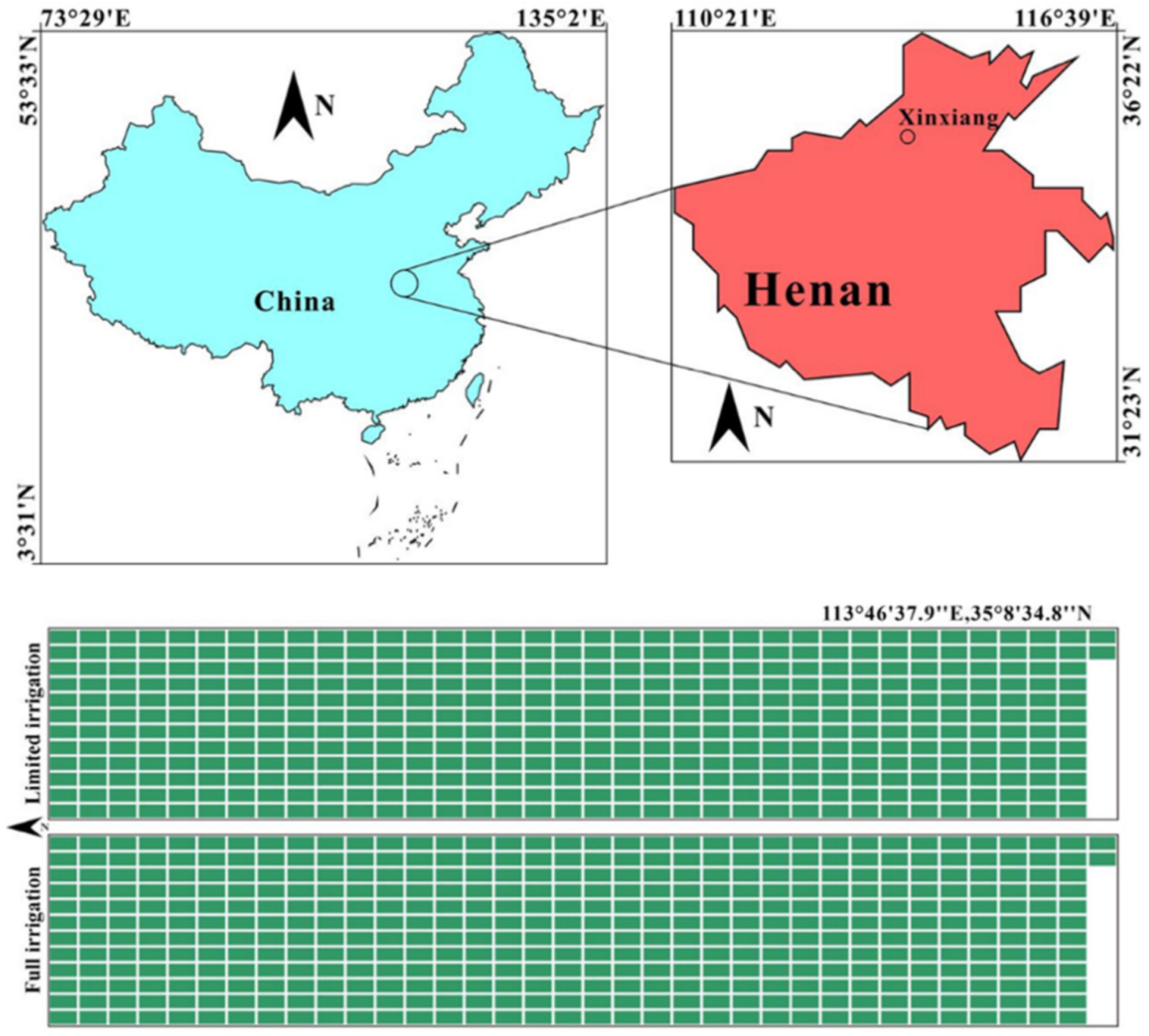
2.1. Plant Materials and Field Trials

Based on a number of UAV-based vegetation indices, a panel of 211 elite winter wheat genotypes was exploited to evaluate the ensemble learning models for grain yield prediction, where 186 accessions were collected from the Yellow and Huai Valleys Winter Wheat Zone (YHVWWZ) of China and 25 from five other countries.
The experiment was conducted at Xinxiang (35°18′N, 113°52′E), Henan province of China during the 2019–2020 cropping season (Figure 1). The genotypes were planted under two irrigation treatments (i.e., full irrigation and limited irrigation) in randomized complete blocks (RCBD) with two replications. A total of 844 plots were phenotype under both irrigation treatments using UAV platform. Each plot consisted of six rows with a length of 3 m, a width of 1.4 m, and inter-row spacing of 0.2 m. The trials were planted on 26 October 2019 with a seeding rate of 270 seedings/m2 and harvested on 2 June 2020. Both irrigation treatments irrigated equal water at the tillering stages, while the full irrigation treatment also flooded in heading and early grain filling stages with 2250–2700 m3 ha−1 of water. The fertilizer and management of both treatments were optimized equally. In addition, the seasonal precipitation was 110.2 mm, and harvesting was done at full maturity using a combine harvester.

2.2. UAV Platform and Flight Mission

A RedEge MX multispectral sensor (Micasense Parrot, Seattle, WA, USA) (https://wwwy.micasense.com/parrotsequoia) (Accessed: 30 November 2020) was mounted on a DJI M210 (SZ DJI Technology Co., Shenzhen, China) for multispectral imagery. The built-in GPS of the Camera provided the position and orientation of the images for data geo-referencing. The RedEdge MX 4.0 can simultaneously collect images of five different bands with GPS information at specific intervals and with the same resolution. The resolution of blue, green, red, red-edge, and near-infrared bands was 32 nm, 27 nm, 14 nm, 12 nm, and 57 nm (half maximum bandwidth), respectively. The detailed information of the band wavelengths is listed in Table 1. Flights were conducted in clear and cloudless weather conditions between 11:00 a.m. to 2:00 p.m. The UAV flew over the trial area in the fully automatic flight mode set by the DJI GS Pro software (https://www.dji.com/cn/ground-station-pro) (Accessed: 1 December 2020). Images for radiometric calibration of the RedEge MX were captured on the flat ground before and after each flight through a calibrated reflectance panel provided by Micasense. To obtain images with high resolution, the forward and side image overlapping was set to 85% and 80%, respectively. The flight altitude was maintained at 40 m for heading and flowering stages, and at 30 m for early and mid grain filling stages. The ground resolution was around 3 cm for the images taken at the altitude of 40 m and 2.5 cm for the altitude of 30 m. The detailed information of the UAV-based data acquisition is presented in Table 2.
In total, around 2000 to 2500 multispectral images were captured from each flight to make mosaic images. Pix4D mapper (Version 1.4, Pix4d, Lausanne, Switzerland) was exploited for orthomosaic generation after each aerial imagery of the experimental field. Meanwhile, plot segmentation for each image was done through QGIS 3.1.0 (https://www.qgis.org/) (Accessed: 30 November 2020). The polygon shapes with a specific ID were designed as masks to extract the spectral data of each plot. The spectral information was extracted using the computer vision algorithms provided by the ENVI software [5].

2.3. Vegetation Indices and Ground Data

As listed in Table 3, twenty vegetation indices were calculated as secondary traits to predict the grain yield. Most of the VIs contain near-infrared and red bands that have been used to quantify the biomass, pigment content, etc. in many crops. Grain yield was estimated for each plot after it was harvested at full maturity.

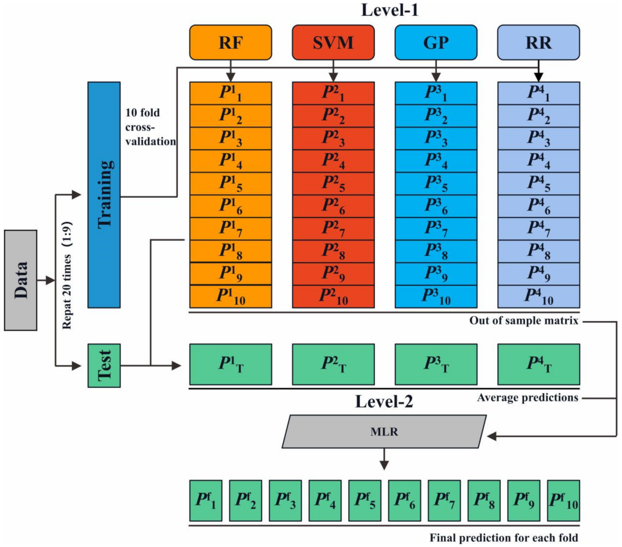
2.4. Stacking Regression Models for Ensemble Learning

Ensemble learning is a machine learning paradigm where multiple base learners are integrated to solve regression or classification problems. Stacking regression is an ensemble learning model proposed by Wolpert (1992) [40] to blend the predictors and improve prediction accuracy. It is commonly used to generate ensembles of heterogeneous predictors. In this study, four regression models including random forest (RF) [24], support vector machine (SVM) [25], Gaussian process (GP) [26], and ridge regression (RR) [27] were integrated for stacking regression-based ensemble learning. The R package “caret” (version 6.0−86) in R 4.0.2 (https://CRAN.R-project.org/package=caret) (Accessed: 30 November 2020) is exploited to build the base learners and the stacking regression framework. The fundamental of stacking regression is illustrated in Figure 2. The data pairs, canopy multispectral reflectance, and grain yield were randomly and evenly split into ten parts, and then one of the parts was used for the test. The predictions for each fold were made by training the model and performing tenfold cross-validation. Based on this, an out-of-sample predictions matrix (OSPM) was obtained. During the tenfold cross-validation, grain yield predictions of each regression model were generated separately to check the results of the base learner on the test set before they were averaged. An OSPM with a dimension of m × n (m is the number of base learners, and n is the number of samples in the training set) was obtained after the m base learners completed the above process. Then, the OSPM was used to train the level-2 regression model to make final predictions. The multiple linear regression (MLR) was used as the level-2 model to avoid collinearity among the prediction results for grain yield. The tenfold cross-validations were also conducted for the level-2 model to reduce uncertainty in prediction results. Especially, the same split process (with tenfold cross-validation) was performed in all models to ensure fair comparisons between the methods. To avoid uncertainty in results, the process of dividing data into training and test sets was repeated 20 times with tenfold cross-validation. This process generated 200 models, and the average prediction accuracy of these 200 models in the test set was taken as the final evaluation index.

2.4.1. Random Forest

Random forest (RF) regression can be regarded as a machine learning model that combines a large number of regression trees [24]. The final output prediction results are the averaged value of all the trees. Regression trees represent a set of conditions or restrictions, and these trees are constructed by bootstrap sampling from a training sample set. This construction strategy overcomes the shortcomings of data and is easy to overfit in the case of complex trees. The key step in constructing an RF is splitting regression trees, and the splitting criterion is based on selecting the input variable with the lowest Gini Index:
I G t X x i = 1 j = 1 m f t X x i , j 2

2.4.2. Support Vector Machine

Support vector machine (SVM) is derived from statistical learning theory and the minimum structural risk principle. SVM is widely applied to data analysis and pattern recognition [25]. The purpose of SVM is to minimize the error by adding a hyperplane and maximizing the margin between positive and negative samples in the training set. The introduction of the loss function allows SVM to solve nonlinear regression problems. Support vector regression can be defined as follows:
f x = i = 1 n a ^ i a i k x i , x + b
where a represents the additional hyperplane alongside the regression line; k (xi, x) is the kernel function, and b is the bias.

2.4.3. Gaussian Process

Gaussian process (GP) is a type of probabilistic kernel machine based on Bayesian and statistical learning theory [26]. It has been extensively used in the field of machine learning. In probability theory and mathematical statistics, GP stands for the observed values in a continuous domain (such as time or space), and it can be regarded as the distribution and inference in a function space. In the process of prediction, GP maximizes the type-II maximum likelihood through the boundary likelihood of observations. In addition, it adjusts the hyperparameters and calculates the posterior distribution of unknown observations. When the observed variable space of GP belongs to a real field, a regression can be conducted to make predictions.

2.4.4. Ridge Regression

Ridge regression was proposed by Tikhonov in 1943 [27] and generalized by Hoerl and Kennard in 1970 [62]. It shrinks the regression coefficients by penalizing them or constraining their possible values. Specifically, ridge regression minimizes the sum of squared errors including an L2-norm penalty on the size of the parameter estimates. The coefficient estimates are, and the corresponding formula is as follows:
β ^ R R =   β   arg   min i = 1 N y i β ^ 0 j = 1 p x i j B ^ j 2 + λ j = 1 p β ^ j 2  
where   λ controls the amount of shrinkage; N represents the number of observations; y is the dependent variable; p and B ^ j   are the number of independent variables and the value of the jth coefficient, respectively.

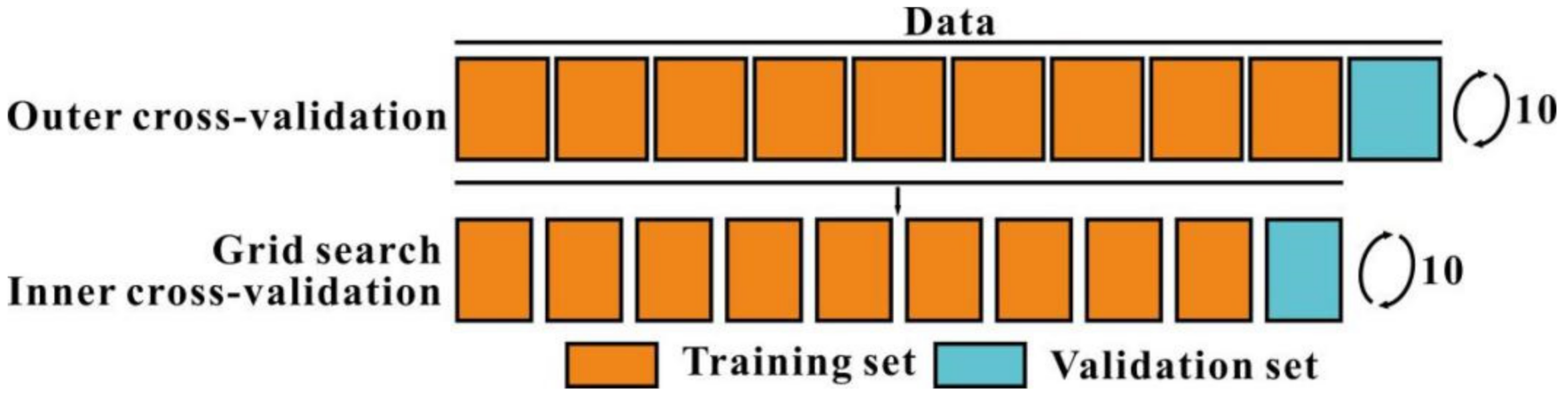
2.4.5. Cross-Validation and Hyperparameter Tune

At level-1 of the stacking regression, the tenfold cross-validation was exploited to form a sample matrix, and this procedure is considered as outer cross-validation. Meanwhile, the inner cross-validation and grid search were conducted to fine-tuning the hyperparameters of the base learners shown in Figure 2. In the outer cross-validation, the original data set was randomly divided into 10 equal subsets (Figure 3). Each time, one of the subsets was used for validating, and the remaining nine subsets for training. Each training set used for the outer cross-validation was also randomly and evenly split into 10 sets, with 10% of the data in the inner validating set and the remaining 90% in the inner training set. In the inner cross-validation, different combinations of candidate hyperparameters were set to construct the model on the inner training set. Then, the constructed model was validated on the inner validating set. Each hyperparameter combination was validated 10 times, and the hyperparameter combination with the highest average validation accuracy on the outer training set was transferred to the outer cross-validation to train the ideal model. The detailed hyperparameters of each machine learning are listed in Table 4.

2.5. Model Performance Evaluation

To evaluate the model performance for grain yield prediction, the coefficients of determination (R2) and root mean square error (RMSE) were calculated through the following equations:
R 2 = 1 i = 1 n y i y ^ i 2 i = 1 n y i y ¯ 2
R M S E = 1 n i = 1 n y i y ^ i 2
where n is the number of samples; y i and y ^ i are the measured and the predicted grain yield of sample i, respectively; y ¯ represents the mean of the measured grain yield. The model with a higher value of R2 and lower values of RMSE can predict grain yield better.

2.6. Statistical Analysis
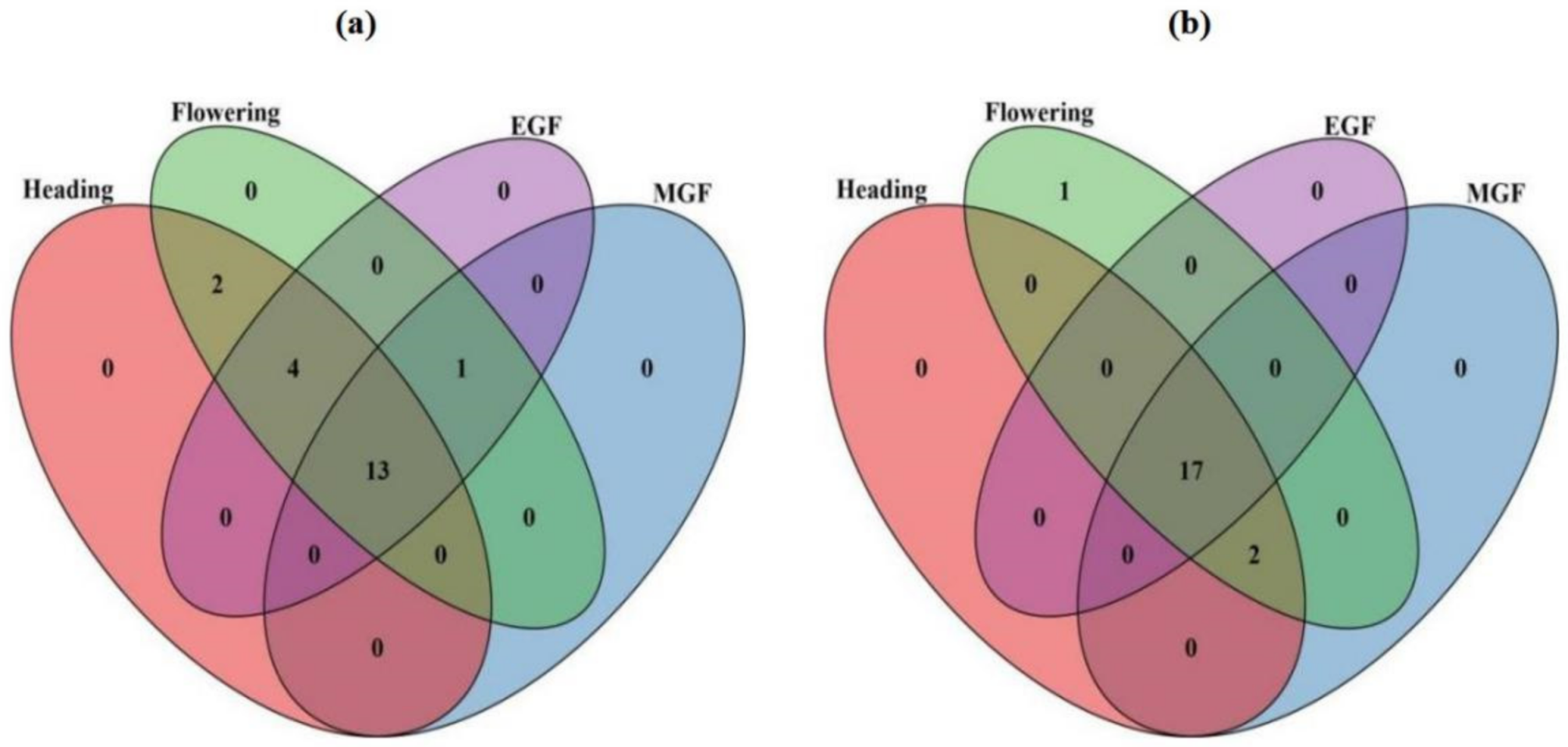
A mixed linear model was exploited to test the significance of variation between genotypes, irrigation treatments, and their interactions for vegetation index and grain yield. The model is presented as follows:
Y = Xβ + Zµ + ε
where Y represents the response demonstrated by fixed effect (β) and random effect (µ) with random error (ε). X and Z are fixed and random effects, respectively. Heritability was estimated through the following formula:
H2 = σg2/(σg2 + σε2/r)
where r is the number of replicates per treatment; σg2 and σε2 indicate the genotypic and error variances, respectively [63]. The spectral traits with low heritability were considered as noise features in previous studies [4]. In this study, the VIs with heritability less than 0.5 were not used as the input features to construct grain yield prediction models.

3. Results

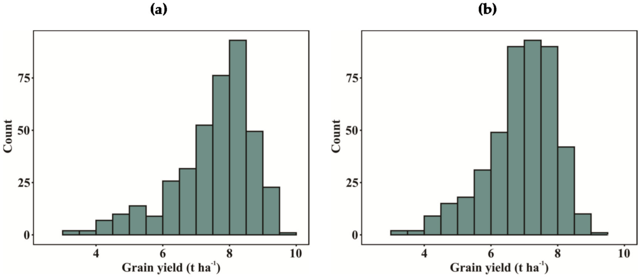
3.1. Phenotypic Analysis

The distribution of averaged grain yield data of irrigation treatments is given in Figure 4. The grain yield under limited irrigation treatment was 8% less than that under full irrigation treatment. It can be seen from the results listed in Table A5 that the coefficient of variation (CV) under full irrigation treatment was 15.7%, which was slightly higher than that under limited irrigation treatment (14.6%). The analysis of variation (ANOVA) results revealed significant variations (p < 0.001) among the genotypes for all vegetation indices (VIs) across the growth stages and grain yield. In addition, there was a significant difference between the two irrigation treatments for all traits (Table A1, Table A2, Table A3, Table A4 and Table A5).
The heritability (H2) was high in the mid-grain filling stage, which ranged from 0.60 to 0.91 for all VIs (Table A1, Table A2, Table A3 and Table A4). The VIs with heritability values greater than 0.5 were selected as the input features for the model to make grain yield prediction for wheat in a particular growth stage. Under full irrigation treatment, the numbers of VIs with a heritability value greater than 0.5 were 17, 14, 18, and 20 for heading flowering EGF and MGF, respectively, and the the numbers of VIs with a heritability value greater than 0.5 under limited irrigation treatment were 19, 19, 18, and 20 across growth stages (Figure 5).

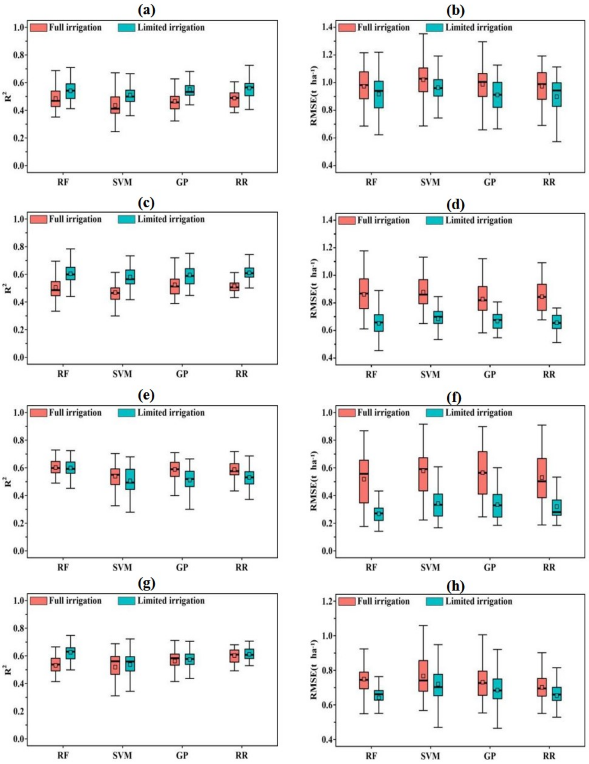
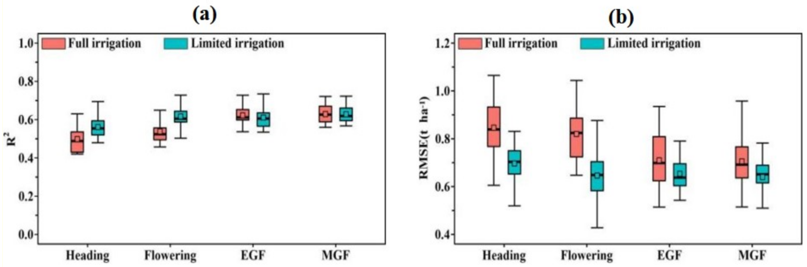
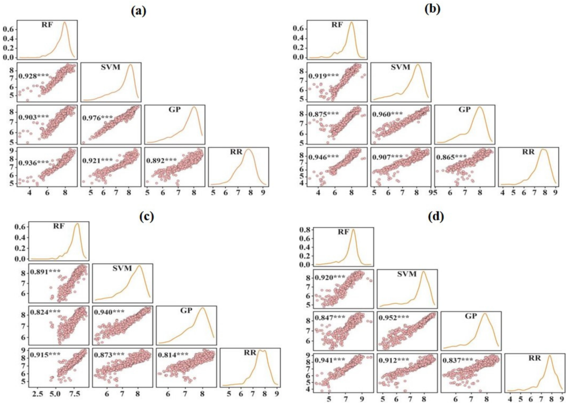
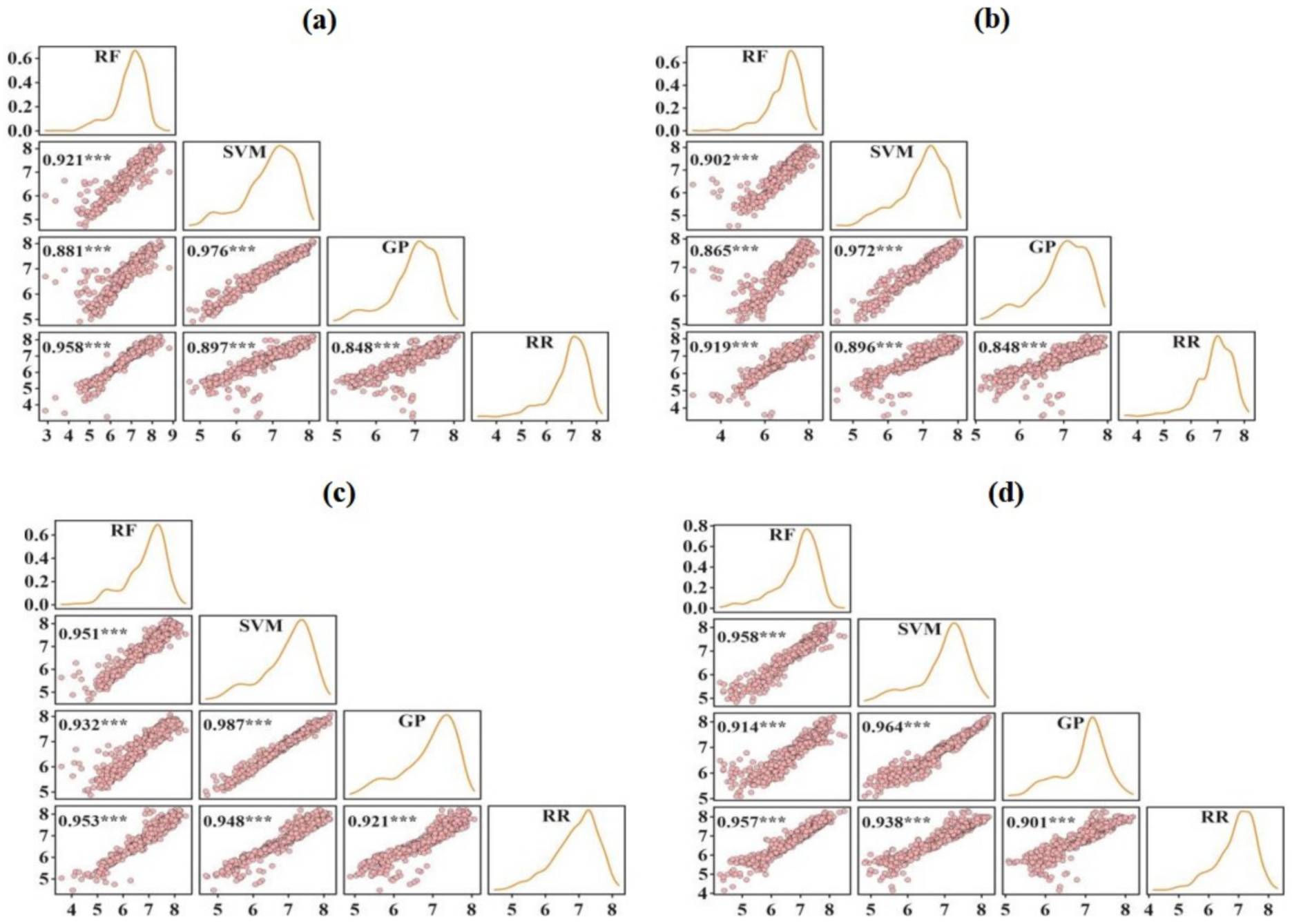
3.2. Performance Base Learners for Grain Yield Prediction

Under full irrigation treatment, the individual base learners achieving the best yield prediction results for the four growth stages are as follows: RR with mean R2 of 0.488 and mean RMSE of 0.859 t ha−1 for the heading stage; GP with mean R2 of 0.520 and mean RMSE of 0.831 t ha−1 for the flowering stage; RF with mean R2 of 0.602 and mean RMSE of 0.711 t ha−1 for the early grain filling stage, and RR with mean R2 of 0.604 and mean RMSE of 0.777 t ha−1 for the mid grain filling stage (Figure 6 and Table 5). SVM did not achieve the best predictions for any of the growth stages. Under limited irrigation treatment, the individual base learners achieving the best yield prediction results for the four growth stages are as follows: RR with mean R2 of 0.561 and mean RMSE of 0.699 t ha−1 for the heading stage; RR with mean R2 of 0.611 and mean RMSE of 0.660 t ha−1 for the flowering stage; RF with mean R2 of 0.599 and mean RMSE of 0.668 t ha−1 for the early grain filling stage, and RF with mean R2 of 0.626 and mean RMSE of 0.641 t ha−1 for the mid grain filling stage. In addition, it can be seen that the prediction results under limited irrigation treatment were slightly higher than those under full irrigation treatment.
As shown in Figure A1 and Figure A2, the Pearson’s correlations between the grain yield from predictions generated by the machine learning algorithms across the four growth stages and the two irrigation treatments were high (r = 0.81–0.97). By contrast, the density curves of the grain yield predictions were slightly different from each other. Moreover, the base learners differed significantly in the distribution interval of the prediction accuracy.

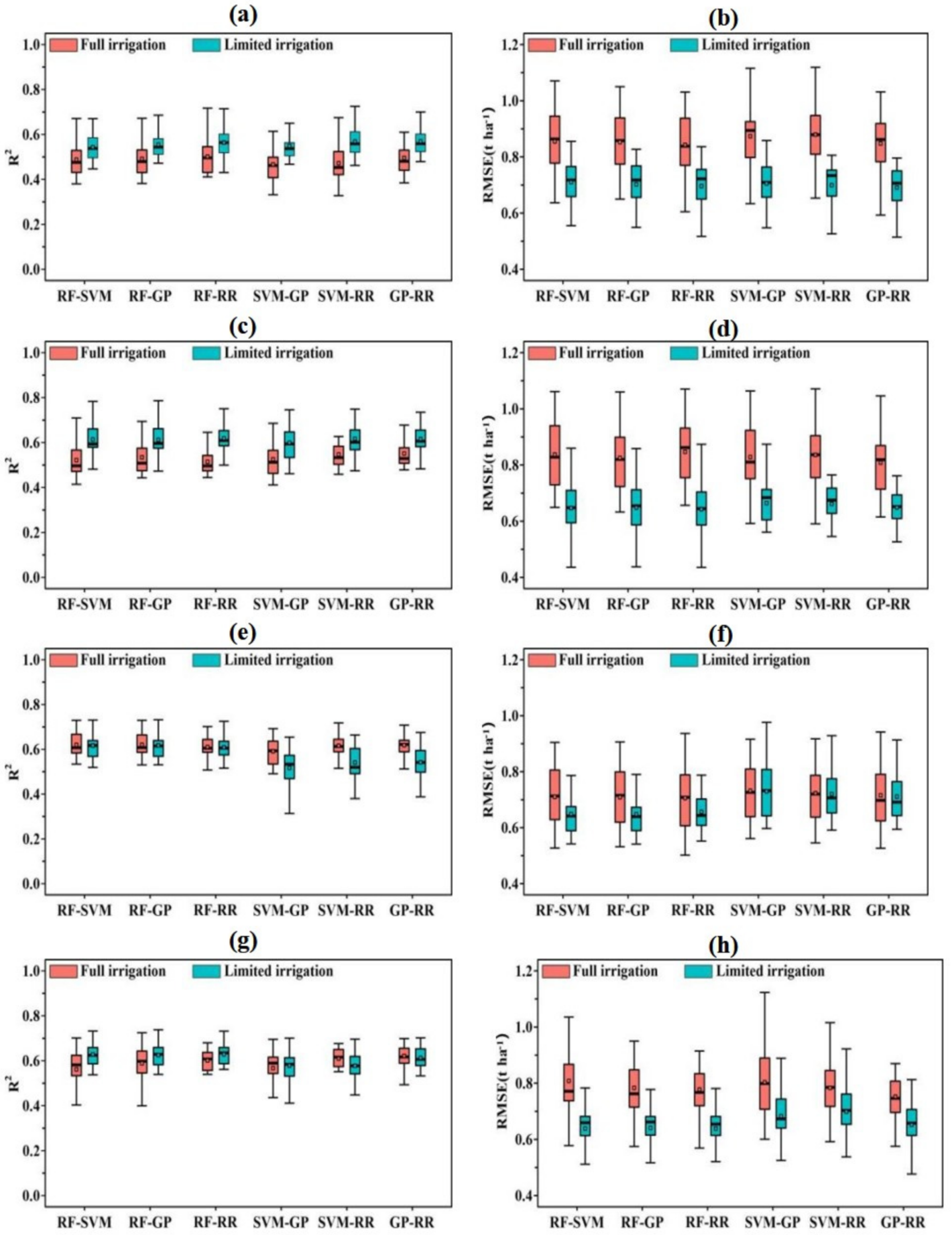
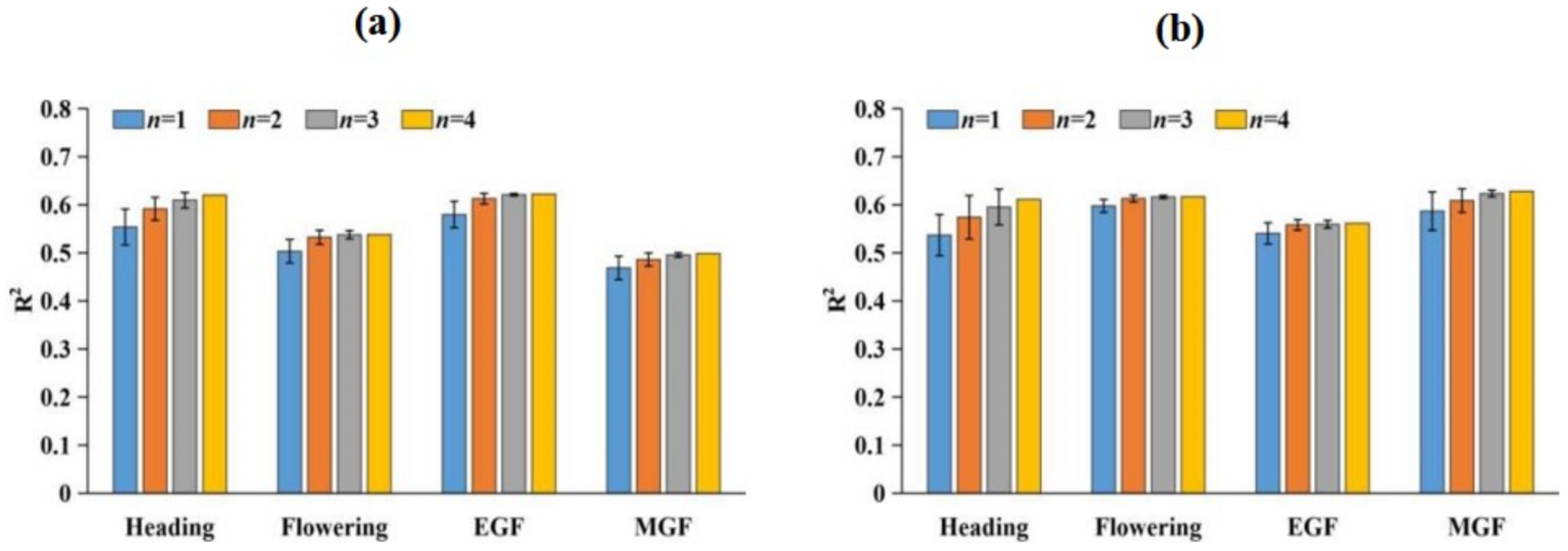
3.3. Ensemble Approach for Grain Yield Prediction

To evaluate the performance of the stacking method, the grain yield prediction is obtained by using different combinations of the base learners for the four growth stages and the two irrigation treatments. The grain yield prediction results obtained by combining two of the base learners are presented in Figure 7 and Table 5. The model combinations achieving the best mean prediction results for the four growth stages under full irrigation treatment are as follows: RF-RR with mean R2 of 0.502 and mean RMSE of 0.843 t ha−1 for the heading stage, GP-RR with mean R2 of 0.551 and mean RMSE of 0.808 t ha−1 for the flowering stage, RF-GP with mean R2 of 0.620 and mean RMSE of 0.709 t ha−1 for the early grain filling stage, and GP-RR with mean R2 of 0.622 and mean RMSE of 0.752 t ha−1 for the mid grain filling stage. The model combinations achieving the best mean prediction results for the four growth stages under the limit irrigation treatment are as follows: GP-RR with mean R2 of 0.570 and mean RMSE of0.691 t ha−1 for the heading stage, RF-RR with mean R2 of 0.619 and mean RMSE of 0.643 t ha−1 for the flowering stage, RF-GP with mean R2 of 0.618 and mean RMSE of 0.648 t ha−1 for the early grain filling stage, and RF-RR with mean R2 of 0.629 and mean RMSE of 0.639 t ha−1 for the mid grain filling stage.
As for the stacking regression combing three base learners, the model combinations with high values of R2 and lowest value of RMSE for the four growth stages under full irrigation treatment are as follows: RF-GP-RR with mean R2 of 0.500 and mean RMSE of 0.845 t ha−1 for the heading stage, SVM-GP-RR with mean R2 of 0.546 and mean RMSE of 0.813 t ha−1 for the flowering stage, RF-SVM-RR with mean R2 of 0.624 and mean RMSE of 0.709 t ha−1 for the early grain filling stage, and SVM-GP-RR with mean R2 of 0.623 and mean RMSE of 0.752 t ha−1 for the mid grain filling stage (Figure 8). The model combinations under limited irrigation treatment, the model combinations achieving the best mean prediction results for the four growth stages under full irrigation treatment are as follows: RF-GP-RR with mean R2 of 0.568 and mean RMSE of 0.693 t ha−1 for the heading stage, RF-SVM-RR with mean R2 of 0.620 and mean RMSE of 0.643 t ha−1 for the flowering stage, RF-SVM-GP with mean R2 of 0.615 and mean RMSE of 0.650 t ha−1 for the early grain filling stage, and RF-SVM-GP with mean R2 of 0.628 and mean RMSE of 0.639 t ha−1 for the mid grain filling stage.
Figure 9 shows the performance of the stacking regression combing all the four base machine learning models for grain yield prediction of the four growth stages. Under full irrigation treatment, the mean values of R2 for the stacking regression were improved to 0.498, 0.538, 0.622, and 0.620 for the heading stage, flowering stage, early grain filling stage, and mid-grain filling stage, respectively. Meanwhile, the mean values of RMSE were reduced to 0.851 t ha−1, 0.820 t ha−1, 0.709 t ha−1, and 0.713 t ha−1 for the heading stage, flowering stage, early grain filling stage, and mid-grain filling stage, respectively. Similar findings were also observed under limited irrigation treatment. The mean values of R2 were up to 0.562, 0.617, 0.611, and 0.628, and the mean values of RMSE were 0.702 t ha−1, 0.647 t ha−1, 0.651 t ha−1, and 0.642 t ha−1, for the heading stage, flowering stage, early filling stage, and mid-grain filling stage, respectively. We estimated the spatial distribution of the grain yield at the plot scale based on the ensemble model by combining four base learners at mid grain filling. The difference of grain yield under the two irrigation treatments can be observed directly in Figure A3.
In terms of the mean R2 and RMSE, most of the ensemble models achieved higher prediction accuracy than the individual best models (Table 5), which confirmed the effectiveness of the ensemble model implemented in this study. In addition, the overall accuracy indicated that the prediction performance of the ensemble model was proportional to the number of base learners (Figure 10).

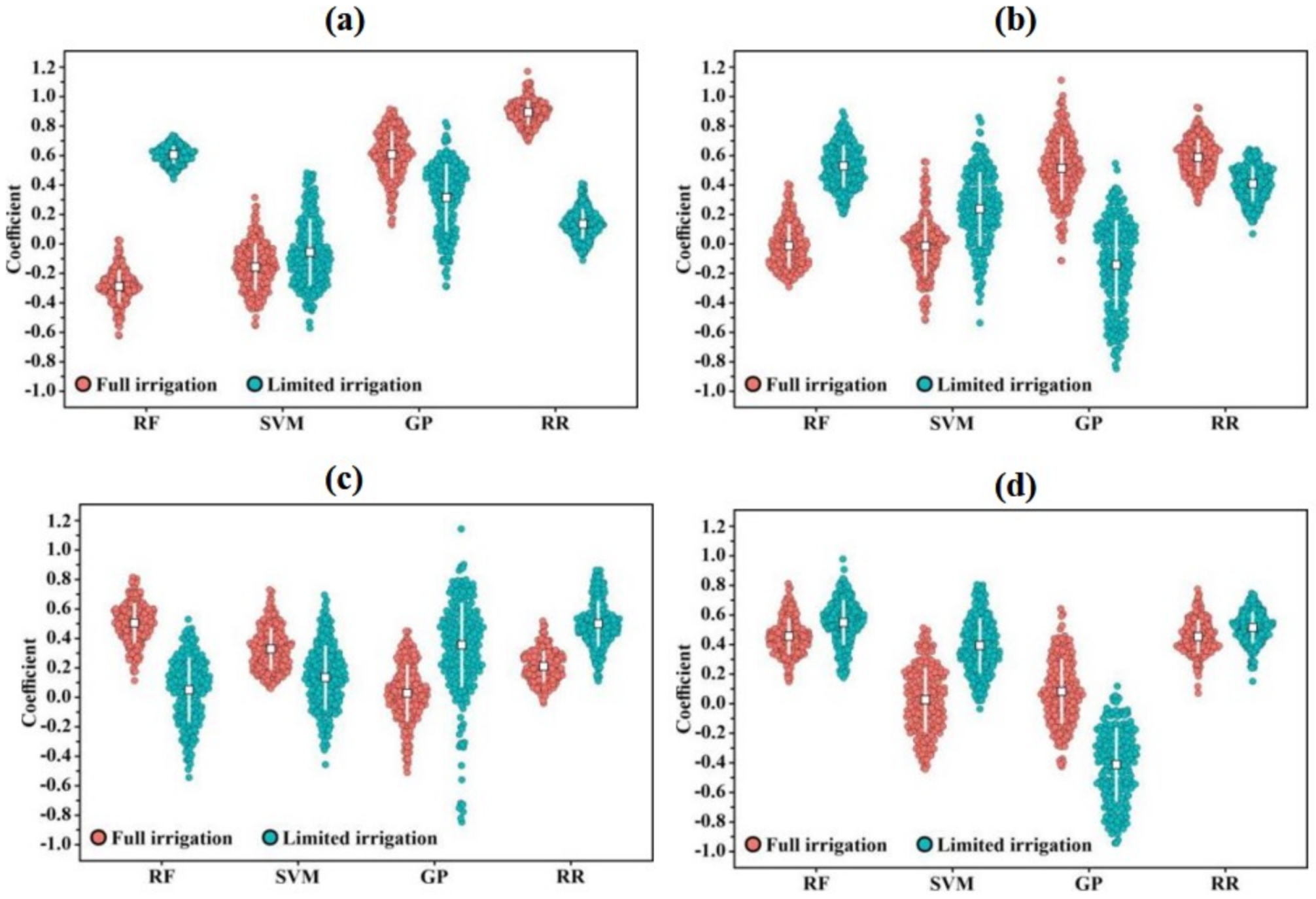
3.4. Regression Coefficient Results for a Secondary Model

Figure 11 illustrates the distribution of the regression coefficients for the four base learners within the secondary model (MLR). A higher regression coefficient of a particular base learner indicated a larger weight in the stacking procedure. Under full irrigation treatment, the stacking performance for the heading stage was strongly influenced by the RR and GP models with high mean regression coefficients of 0.89 and 0.61, respectively. Similar results were observed for the flowering stage, where the mean regression coefficients of the RR and GP were 0.59 and 0.51, respectively. The impacts of the RF and SVM models on the stacking regression were relatively small with the mean regression coefficients of −0.01 and −0.02, respectively. The RF had the highest impact on the stacking performance for the early grain filling stage with a mean regression coefficient of 0.50, followed by the SVM with a mean regression coefficient of 0.33, RR with a mean regression coefficient of 0.03, and GP with a mean regression coefficient of 0.21. For the mid-grain filling stage, the RF and RR models had similar weights with the mean regression coefficients of 0.46 and 0.45, respectively, followed by the GP and SVM with the mean regression coefficients of 0.08 and 0.03. Under limited irrigation, RF showed a higher influence on the stacking performance with a mean regression coefficient of 0.61, while the GP, RR, and SVM models had mean regression coefficients of 0.31, 0.14, and −0.06, respectively. For the flowering stage, early grain filling stage, and mid-grain filling stage, the impact of the RF-based model was with the regression coefficient of 0.53, 0.55, and 0.05, respectively; the impact of the RR-based model was with the regression coefficient of 0.41, 0.52, and 0.50, respectively; the impact of SVM-based model was with the regression coefficient of 0.24, 0.39, and 0.13, respectively, the impact of GP-based model was with the regression coefficient of −1.14, −0.41, and 0.36, respectively. Overall, the results indicated that the stacking regression achieved higher prediction accuracy by allocating a more reasonable weight of base learners under various modeling conditions.

4. Discussion

The UAV-based multispectral vegetation indices have been increasingly exploited to predict plant physiological traits by crop breeding studies [5,64]. In this study, 20 VIs covering all five light bands captured by the multispectral sensor were taken to evaluate the machine learning models for grain yield prediction. The high heritability of the VIs indicated an excellent accuracy of these traits for grain yield prediction (Table A1, Table A2, Table A3 and Table A4). Among these VIs, GNDVI, NDRE, OSAVIREG, MSRREG, and MTCI had a heritability greater than 0.5 under both the treatments and across the growth stages. These five VIs could be selected as the best ones to predict variations among the genotypes for grain yield. Previously, some studies have reported that GNDVI and NDRE were the best predictors for grain yield and nutrient uptake efficiencies across the growth stages [5,64]. Therefore, these VIs can be used to select high-yielding genotypes with high accuracy in large breeding programs. Concerning water stress condition between different irrigation treatments, it has been found that thermal images show a correlation between minor changes in water stress that are undetectable by the multispectral indices as normalized difference vegetation index (NDVI) [65]. Thermal imagery can help diagnosis of water stress in plants, causes by the stomatal closure, which determines the reduction of the transpiration rate and decreasing evaporative cooling increases leaf temperature. In this regard, canopy thermal imaging represents a fast and practical way to evaluate and estimate crop water status, indicating plant’s water content. In some cases, relationship of canopy temperature has also been reported high with grain yield at early grain filling stages but lower at later grain fulling stages [66]. This might be due to low greenness and photosynthetic activity at late maturation stages. When wilting starts and transpiration decreases, the temperature difference between plots could get small which weakened the discrimination ability of canopy temperature at plot level growth. Therefore, data fusion of multispectral and canopy temperature imagery for GY prediction at a critical growth stage can increase the accuracy of prediction analysis. Meanwhile, the introduction of machine learning models can further improve the prediction accuracy and decisions during selection. To achieve precise prediction results and reduce the risk of overfitting, machine learning algorithms usually adopted feature selection strategies to reduce the data dimension to a suitable level [34]. In this study, VIs with heritability greater than 0.5 were selected across the growth stages, which means that all the base learners and their combinations were evaluated at maximum input data accuracy and repeatability. Previously, feature selection algorithms such as recursive feature elimination (RFE) [37] and Boruta [67] have been applied to prediction analysis. Different from RFE and Boruta, the feature selection based on heritability can be performed without knowing the predictor variables in breeding work. The successful use of heritability to reduce the number of input features has been reported in the previous study [4], and it achieved high prediction accuracy. Therefore, taking VIs with high heritability as input data increased the prediction accuracy and reliability of the models to assess the variations of genotypes.
Previously, several studies have exploited different machine learning models such as RR, SVM, RF, and GP to predict grain yield and physiological attributes of plants on remote sensing data sets [32,33,34,35,36]. This study aims to evaluate the combination of the above base learners to form an ensemble learning approach for grain yield prediction in different growth stages. It is difficult for a single machine learning model to predict several plant attributes using similar algorithms. For example, random forest algorithms are among the most powerful machine learning algorithms because of their proven accuracy, adaptability, and simplicity [32]. Such algorithms have been used in applications ranging from forest growth monitoring to winter wheat leaf chlorophyll content estimation [32,68]. However, the model performance of random forest is not as good as ridge regression in most cases considered by this study. Different characteristics of trait composition made it difficult for an algorithm of any model to maintain the prediction ability and accuracy in the case of several varied traits as input data [34,37]. The RR model has been reported to have high accuracy and robustness under most of the modeling conditions [69,70,71,72]. In our study, better prediction results were also obtained by the RR model compared to other models (Figure 6 and Table 5). It might be attributed to the biased nature of the model for collinear data analysis and comprehensive relationship for most of the traits [69,73]. However, the prediction ability of the RR model could be low in some cases, due to traits, growth stages, and growing conditions [74]. Therefore, it is important to find a method that can combine the advantages of multiple models to achieve an improved prediction accuracy under various growth conditions for grain yield prediction.
Ensemble learning approaches have been reported to increase the diversity of algorithms by combining different base learners, and the combination of more heterogeneities of base learners improves the ensemble learning model with higher prediction ability. When implementing a stacking method, it is necessary to include self-sufficient, independent, and diverse base learners for analysis [34,37]. In this study, four machine learning algorithms with different principles and internal structures were successfully combined, which achieved higher accuracy for predicting grain yield than the single base learner. In addition, the accuracy parameters (R2 and RMSE) of the base learners exhibited more fluctuations with the wide ranges than that of the ensemble approaches (Figure 7, Figure 8 and Figure 9), indicating the stability of the ensemble approaches on new data.
Among all the combinations with two, three, and four base learners, the one that contained the RR model performed well in terms of prediction accuracy across growth stages and treatments. Meanwhile, the regression coefficient analysis of combining the four base learners showed a higher weight of RR in most of the cases. Therefore, the RR model had a great influence on the ensemble method for grain yield prediction. Combining two or three base learners can contribute to higher prediction accuracy than combining four base learners in some cases, but these model combinations were unstable and performed poorly in other situations. Conversely, the model combination of four base learners exhibited good accuracy and stability in all the cases, which is of great significance to the practical applications of the prediction model. Overall, the stacking regression method can achieve higher prediction accuracy than individual base learners, and the improvement was proportional to the number of base learners (Figure 10). This is consistent with the conclusion of a previous study for estimating hourly and continuous ground-level PM2.5 concentrations [44]. The stacking regression can be further optimized for grain yield prediction. The results of this study showed that the larger the number of base learners, the higher the accuracy of the final model (Figure 10). It means that more machine learning algorithms should be incorporated by the stacking regression method. Therefore, deep learning-based regression methods such as multilayer perceptron (MLP) [75] can be used as a new algorithm in the stacking procedure, while multiple birth SVM regression [76] and parallel RF regression [77] can be respectively used as variants of the SVM and RF regression for further improvement of the model. In addition, stacking a large number of base learners requires a level-2 model to perform the multicollinearity data analysis in the model [78]. Thus, ridge regression, least absolute shrinkage, selection operator (LASSO), and elastic net regression (ENET) can be used as level-2 models for collinearity analysis [78,79,80,81]. The grain yield predictions made by single models under full and limited irrigation treatments were similar across the growth stages, indicating the adaptability of UAV data for grain yield prediction. The prediction results obtained from ensemble learning were very similar under both irrigation treatments i.e., full irrigation treatment (R2 = 0.625) and limited irrigation treatment (R2 = 0.628) at the mid-grain filling stage. This result indicated that the mid-grain filling stage is the most appropriate stage to predict the grain yield under full and limited irrigation treatments. This is rational since grain filling is the stage where wheat transfers organic matter such as starch and protein produced by photosynthesis from the vegetative organs to the grains, and the vegetation indexes in this period are closely related to the final quality of thousand-grain weight [82].

5. Conclusions

Recently, there is an increasing focus on using multi-model fusion for data analysis to increase the prediction accuracy in crops. We have successfully used the ensemble learning method to stack the multiple base leaners to increase the grain yield prediction accuracy in wheat. The experimental results showed that the stacking of multi base learners possess the capability to improve the traits estimations effectively as compared to simple regression methods. Since UAV based phenotyping platforms can estimate spectral information from multiple growth stages cost-effectively, the use of ensemble learning approaches is important in increasing the accuracy of within season yield predictions. Our results illustrated the usefulness of ensemble learning approach for yield prediction using multi-stage multispectral data. We also demonstrated the weight of each base leaner such as random forest (RF), support vector machine (SVM), Gaussian process (GP), and ridge regression (RR) in ensemble leaning model development for yield prediction. Grain yield prediction results were high at a mid grain filling stage when a four base learner combination was used in an ensemble learning model as compared to other growth stages and base leaner combinations. To date, relatively few studies have been done to use the information obtained by UAV based sensors as inputs in ensemble learning model prediction of grain yield in winter wheat. Further validations of ensemble learning methods on multiple crops and UAV based data are required to increase its validity and authenticity in crop breeding.

Author Contributions

S.F. and M.A.H. collected the data, analyzed the data, and wrote the paper under the supervision of C.L., Y.X. managed and directed the trial. M.S., Z.C., Z.H., and J.W. gave comments and suggestions to improve the manuscript. All authors have read and agreed to the published version of the manuscript.

Funding

This work was funded by the Fundamental Research Funds for the Institute Planning in the Chinese Academy of Agricultural Sciences (S2018QY02), and the National Natural Science Foundation of China (31671691, 3171101265).

Institutional Review Board Statement

Not applicable.

Informed Consent Statement

Not applicable.

Data Availability Statement

Data will be available on demand.

Conflicts of Interest

There is no conflict of interest regarding this study.

Appendix A

Table A1. Main statistical parameters of grain yield under two irrigation treatments.
TreatmentMean (t ha−1)CV (%)F-ValueH2
Genotype (G)Treatment (T)G × T
Full Irrigation7.5915.710.401 ***264.432 ***0.980.85
Limited Irrigation6.9214.60.89
***, significant at p < 0.001; CV means coefficient of variation.
Table A2. Significance test and heritability of the vegetation indexes extracted in the heading stage.
Vegetation IndexGenotype (G)Treatment (T)G × TH2
F-ValueF-ValueF-ValueFull IrrigationLimited Irrigation
NDVI4.854 ***743.179 ***1.263 *0.510.78
SAVI4.855 ***743.178 ***1.262 *0.510.78
OSAVI4.856 ***743.226 ***1.262 *0.510.78
NRI4.599 ***1284.147 ***1.344 *0.520.80
GNDVI5.998 ***235.842 ***1.1040.700.74
SIPI3.439 ***564.833 ***1.222 *0.500.62
PSRI1.1480.7711.1560.140.13
CRI7.058 ***7.053 **0.9680.780.72
EVI7.777 ***480.102 ***1.482 **0.820.71
MSR3.952 ***710.450 ***1.0220.470.75
NLI4.184 ***1446.413 ***1.261 *0.440.74
RDVI4.298 ***325.237 ***0.9880.560.73
TVI4.890 ***741.107 ***1.278 *0.510.78
MTVI28.176 ***1005.586 ***1.436 **0.810.76
NDRE17.346 ***139.202 ***1.1660.880.90
DVIREG7.126 ***1302.732 ***0.9280.650.82
OSAVIREG17.346 ***139.204 ***1.1660.880.90
RDVIREG9.764 ***1103.257 ***1.349 *0.730.87
MSRREG17.958 ***138.719 ***1.1770.880.91
MTCI17.304 ***184.176 ***1.1870.880.91
*, **, ***, significant at p < 0.05, p < 0.01 and p < 0.001, respectively.
Table A3. Significance test and heritability of the vegetation indexes extracted in the flowering stage.
Vegetation IndexGenotype (G)Treatment (T)G × TH2
F-ValueF-ValueF-ValueFull IrrigationLimited Irrigation
NDVI6.436 ***948.477 ***1.408 *0.710.77
SAVI6.436 ***948.481 ***1.408 *0.710.77
OSAVI6.436 ***948.440 ***1.408 *0.710.77
NRI3.687 ***502.703 ***1.1320.590.57
GNDVI6.622 ***740.962 ***1.463 **0.730.78
SIPI5.619 ***2053.124 ***1.565 ***0.670.75
PSRI1.1532.0171.1580.640.13
CRI1.929 ***3.6241.281 *0.340.54
EVI1.725 ***154.691 ***1.481 **0.350.51
MSR5.995 ***1008.409 ***1.371 *0.700.76
NLI3.189 ***694.061 ***1.511 **0.460.72
RDVI2.950 ***253.226 ***1.1950.440.70
TVI6.458 ***937.304 ***1.413 *0.710.77
MTVI22.009 ***292.869 ***1.487 **0.390.59
NDRE10.989 ***35.906 ***1.0440.770.91
DVIREG3.525 ***244.143 ***1.347 *0.490.80
OSAVIREG10.989 ***35.908 ***1.0440.770.91
RDVIREG4.918 ***209.064 ***1.526 ***0.560.85
MSRREG11.078 ***34.183 ***1.0460.770.91
MTCI10.682 ***73.627 ***1.0530.770.90
*, **, ***, significant at p < 0.05, p < 0.01 and p < 0.001, respectively.
Table A4. Significance test and heritability of the vegetation indexes extracted in the early grain filling stage.
Vegetation IndexGenotype (G)Treatment (T)G × TH2
F-ValueF-ValueF-ValueFull IrrigationLimited Irrigation
NDVI6.407 ***131.876 ***1.484 **0.690.79
SAVI6.407 ***131.873 ***1.484 **0.690.79
OSAVI6.407 ***131.889 ***1.484 **0.690.79
NRI5.019 ***906.706 ***1.424 **0.510.79
GNDVI9.13 ***45.687 ***1.452 **0.790.83
SIPI7.784 ***17.953 ***1.705 ***0.750.83
PSRI1.1560.3031.1620.750.13
CRI5.786 ***442.256 ***1.0820.690.72
EVI4.652 ***751.814 ***1.1290.640.67
MSR5.834 ***139.053 ***1.327 *0.650.79
NLI3.265 ***812.713 ***1.1440.450.56
RDVI5.635 ***2.0481.1040.640.78
TVI6.404 ***131.186 ***1.49 **0.690.78
MTVI24.417 ***886.16 ***1.1060.600.66
NDRE19.785 ***67.904 ***1.349 *0.880.93
DVIREG2.376 ***450.393 ***0.8040.370.35
OSAVIREG19.785 ***67.9 ***1.349 *0.880.93
RDVIREG3.432 ***342.097 ***0.7460.580.48
MSRREG20.303 ***67.16 ***1.375 *0.880.93
MTCI19.822 ***45.575 ***1.401 *0.880.93
*, **, ***, significant at p < 0.05, p < 0.01 and p < 0.001, respectively.
Table A5. Significance test and heritability of the vegetation indexes extracted in the mid-grain filling stage.
Vegetation IndexGenotype (G)Treatment (T)G × TH2
F-ValueF-ValueF-ValueFull IrrigationLimited Irrigation
NDVI9.091 ***1121.021 ***1.365 *0.800.81
SAVI9.091 ***1121.035 ***1.365 *0.800.81
OSAVI9.091 ***1121.020 ***1.365 *0.800.81
NRI4.860 ***1682.199 ***1.275 *0.630.69
GNDVI13.186 ***614.600 ***1.223 *0.860.86
SIPI8.883 ***765.657 ***1.357 *0.780.82
PSRI8.278 ***779.147 ***1.544 ***0.750.81
CRI6.456 ***2.3740.9280.710.76
EVI4.408 ***576.88 ***1.0960.600.68
MSR7.881 ***1353.925 ***1.1040.760.79
NLI5.014 ***1205.454 ***1.1840.620.71
RDVI6.774 ***785.527 ***1.0800.720.79
TVI9.124 ***1073.981 ***1.398 *0.800.81
MTVI24.487 ***791.938 ***1.1130.610.68
NDRE17.429 ***528.708 ***1.0890.880.91
DVIREG8.626 ***997.224 ***1.0440.780.81
OSAVIREG17.429 ***528.698 ***1.0890.880.91
RDVIREG7.046 ***761.566 ***1.1440.730.77
MSRREG18.188 ***526.719 ***1.1060.880.91
MTCI17.312 ***636.939 ***1.1110.880.90
*, **, ***, significant at p < 0.05, p < 0.01 and p < 0.001, respectively.
Figure A1. Regression plots, density curves, and correlation coefficient of the grain yield prediction generated by various machine learning methods at four growth stages under full irrigation treatment; (a) heading stage; (b) flowering stage; (c) early grain filling stage; (d) mid-grain filling stage significant (***) at p < 0.001. Abbreviations: RF, random forest; SVM; support vector machine; GP, Gaussian process; and RR, ridge regression.
Remotesensing 13 02338 g0a1
Figure A2. Regression plots, density curves, and correlation coefficient of grain yield prediction generated by various machine learning methods at four growth stages under limited irrigation treatment; (a) heading stage; (b) flowering stage; (c) early grain filling stage; (d) mid-grain filling stage significant (***) at p < 0.001. Abbreviations: RF, random forest; SVM; support vector machine; GP, Gaussian process; and RR, ridge regression.
Remotesensing 13 02338 g0a2
Figure A3. Spatial distribution of grain yield (t ha−1) at the plot scale using an ensemble learning model.
Remotesensing 13 02338 g0a3

References

  1. Ray, D.K.; Mueller, N.D.; West, P.C.; Foley, J.A. Yield Trends Are Insufficient to Double Global Crop Production by 2050. PLoS ONE 2013, 8, e66428. [Google Scholar] [CrossRef] [PubMed] [Green Version]
  2. Reynolds, M.; Tattaris, M.; Cossani, C.M.; Ellis, M.; Yamaguchi-Shinozaki, K.; Pierre, C.S. Exploring Genetic Resources to Increase Adaptation of Wheat to Climate Change. In Advances in Wheat Genetics: From Genome to Field, Proceedings of the 12th International Wheat Genetics Symposium, Yokohama, Japan, 8–14 September 2013; Ogihara, Y., Takumi, S., Handa, H., Eds.; Springer Science and Business Media LLC: Tokyo, Japan, 2015; pp. 355–368. [Google Scholar]
  3. Lesk, C.; Rowhani, P.; Ramankutty, N. Influence of extreme weather disasters on global crop production. Nature 2016, 529, 84–87. [Google Scholar] [CrossRef] [PubMed]
  4. Montesinos-Lopez, O.A.; Montesinos-Lopez, A.; Crossa, J.; de Los Campos, G.; Alvarado, G.; Suchismita, M.; Rutkoski, J.; Gonzalez-Perez, L.; Burgueno, J. Predicting grain yield using canopy hyperspectral reflectance in wheat breeding data. Plant Methods 2017, 13, 4. [Google Scholar] [CrossRef] [PubMed] [Green Version]
  5. Hassan, M.A.; Yang, M.; Rasheed, A.; Yang, G.; Reynolds, M.; Xia, X.; Xiao, Y.; He, Z. A Rapid monitoring of NDVI across the wheat growth cycle for grain yield prediction using a multi-spectral UAV platform. Plant Sci. 2019, 282, 95–103. [Google Scholar] [CrossRef]
  6. Rutkoski, J.; Poland, J.; Mondal, S.; Autrique, E.; Pérez, L.G.; Crossa, J.; Reynolds, M.; Singh, R. Canopy temperature and vegetation indices from high-throughput phenotyping improve accuracy of pedigree and genomic selection for grain yield in wheat. G3 Genes Genomes Genet. 2016, 6, 2799–2808. [Google Scholar] [CrossRef] [Green Version]
  7. Großkinsky, D.K.; Jesper, S.; Svend, C.; Thomas, R. Plant phenomics and the need for physiological phenotyping across scales to narrow the genotype-to-phenotype knowledge gap. J. Exp. Bot. 2015, 66, 5429–5440. [Google Scholar] [CrossRef] [Green Version]
  8. Furbank, R.T.; Tester, M. Phenomics—Technologies to relieve the phenotyping bottleneck. Trends Plant Sci. 2011, 16, 635–644. [Google Scholar] [CrossRef]
  9. Araus, J.L.; Cairns, J.E. Field high-throughput phenotyping: The new crop breeding frontier. Trends Plant Sci. 2014, 19, 52–61. [Google Scholar] [CrossRef]
  10. Xie, C.; Yang, C. A review on plant high-throughput phenotyping traits using UAV-based sensors. Comput. Electron. Agric. 2020, 178, 105731. [Google Scholar] [CrossRef]
  11. Fenner, H.; Andrew, R.; Adam, M.; March, C.; Martin, W.; Malcolm, H. High Throughput field phenotyping of wheat plant height and growth rate in field plot trials using UAV based remote sensing. Remote Sens. 2016, 8, 1031. [Google Scholar]
  12. Lin, Y.C.; Zhou, T.; Wang, T.; Crawford, M.; Habib, A. New orthophoto generation strategies from UAV and ground remote sensing platforms for high-throughput phenotyping. Remote Sens. 2021, 13, 860. [Google Scholar] [CrossRef]
  13. Di Gennaro, S.F.; Rizza, F.; Badeck, F.W.; Berton, A.; Delbono, S.; Gioli, B.; Toscano, P.; Zaldei, A.; Matese, A. UAV-based high-throughput phenotyping to discriminate barley vigour with visible and near-infrared vegetation indices. Int. J. Remote Sens. 2018, 39, 5330–5344. [Google Scholar] [CrossRef]
  14. Hassan, M.; Yang, M.; Rasheed, A.; Jin, X.; Xia, X.; Xiao, Y.; He, Z. Time-series multispectral indices from unmanned aerial vehicle imagery reveal senescence rate in bread wheat. Remote Sens. 2018, 10, 809. [Google Scholar] [CrossRef] [Green Version]
  15. Zhu, X.; Liu, D. Improving forest aboveground biomass estimation using seasonal Landsat NDVI time-series. ISPRS J. Photogramm. 2015, 102, 222–231. [Google Scholar] [CrossRef]
  16. Prananda, A.; Kamal, M.; Kusuma, D.W. The effect of using different vegetation indices for mangrove leaf area index modelling. IOP Conf. Ser. Earth Environ. Sci. 2020, 500, 012006. [Google Scholar] [CrossRef]
  17. Han, L.; Yang, G.; Dai, H.; Xu, B.; Yang, H.; Feng, H.; Li, Z.; Yang, X. Modeling maize above-ground biomass based on machine learning approaches using UAV remote-sensing data. Plant Methods 2019, 15, 10. [Google Scholar] [CrossRef] [Green Version]
  18. Dahms, T.; Seissiger, S.; Borg, E.; Vajen, H.; Fichtelmann, B.; Conrad, C. Important variables of a rapideye time series for modelling biophysical parameters of winter wheat. Photogramm. Fernerkund. Geoinf. 2016, 2016, 285–299. [Google Scholar] [CrossRef] [Green Version]
  19. Liu, Y.; Cheng, T.; Zhu, Y.; Tian, Y.; Cao, W.; Yao, X.; Wang, N. Comparative analysis of vegetation indices, non-parametric and physical retrieval methods for monitoring nitrogen in wheat using UAV-based multispectral imagery. In Proceedings of the International Geoscience and Remote Sensing Symposium (IGARSS), Beijing, China, 10–15 July 2016; pp. 7362–7365. [Google Scholar]
  20. Sonobe, R.; Sano, T.; Horie, H. Using spectral reflectance to estimate leaf chlorophyll content of tea with shading treatments. Biosyst. Eng. 2018, 175, 168–182. [Google Scholar] [CrossRef]
  21. Gleason, C.J.; Im, J. Forest biomass estimation from airborne LiDAR data using machine learning approaches. Remote Sens. Environ. 2012, 125, 80–91. [Google Scholar] [CrossRef]
  22. Montes, J.M.; Technow, F.; Dhillon, B.S.; Mauch, F.; Melchinger, A.E. High-throughput non-destructive biomass determination during early plant development in maize under field conditions. Field Crop. Res. 2011, 121, 268–273. [Google Scholar] [CrossRef]
  23. Prasad, R.; Pandey, A.; Singh, K.P.; Singh, V.P.; Mishra, R.K.; Singh, D. Retrieval of spinach crop parameters by microwave remote sensing with back propagation artificial neural networks: A comparison of different transfer functions. Adv. Space Res. 2012, 50, 363–370. [Google Scholar] [CrossRef]
  24. Breiman, L. Random forests. Mach. Learn. 2001, 45, 5–32. [Google Scholar] [CrossRef] [Green Version]
  25. Cortes, C.; Vapnik, V. Support-vector networks. Mach. Learn. 1995, 20, 273–297. [Google Scholar] [CrossRef]
  26. Ounpraseuth, S. Gaussian processes for machine learning. J. Am. Stat. Assoc. 2008, 103, 429. [Google Scholar] [CrossRef]
  27. Tikhonov, A.N. On the stability of inverse problems. C.R. Acad. Sci. URSS 1943, 39, 176-170. [Google Scholar]
  28. Wang, L.A.; Zhou, X.; Zhu, X.; Dong, Z.; Guo, W. Estimation of biomass in wheat using random forest regression algorithm and remote sensing data. Crop. J. 2016, 4, 212–219. [Google Scholar] [CrossRef] [Green Version]
  29. Wang, J.; Chen, Y.; Chen, F.; Shi, T.; Wu, G. Wavelet-based coupling of leaf and canopy reflectance spectra to improve the estimation accuracy of foliar nitrogen concentration. Agric. For. Meteorol. 2018, 248, 306–315. [Google Scholar] [CrossRef]
  30. Houborg, R.; McCabe, M.F. A Hybrid training approach for leaf area index estimation via cubist and random forests machine-learning. ISPRS J. Photogramm. Remote Sens. 2018, 135, 173–188. [Google Scholar] [CrossRef]
  31. Zhang, J.; Cheng, T.; Guo, W.; Xu, X.; Qiao, H.; Xie, Y.; Ma, X. Leaf area index estimation model for UAV image hyperspectral data based on wavelength variable selection and machine learning methods. Plant Methods 2021, 17, 49. [Google Scholar] [CrossRef]
  32. Shah, S.H.; Angel, Y.; Houborg, R.; Ali, S.; McCabe, M.F. A random forest machine learning approach for the retrieval of leaf chlorophyll content in wheat. Remote Sens. 2019, 11, 920. [Google Scholar] [CrossRef] [Green Version]
  33. Liang, L.; Geng, D.; Yan, J.; Qiu, S.; Di, L.; Wang, S.; Xu, L.; Wang, L.; Kang, J.; Li, L. Estimating crop LAI using spectral feature extraction and the hybrid inversion method. Remote Sens. 2020, 12, 3534. [Google Scholar] [CrossRef]
  34. Yoosefzadeh-Najafabadi, M.; Earl, H.J.; Tulpan, D.; Sulik, J.; Eskandari, M. Application of machine learning algorithms in plant breeding: Predicting yield from hyperspectral reflectance in soybean. Front. Plant Sci. 2021, 11, 624273. [Google Scholar] [CrossRef]
  35. Xie, R.; Darvishzadeh, R.; Skidmore, A.K.; Heurich, M.; Holzwarth, S.; Gara, T.W.; Reusen, I. Mapping leaf area index in a mixed temperate forest using fenix airborne hyperspectral data and gaussian processes regression. Int. J. Appl. Earth Obs. Geoinf. 2021, 95, 102242. [Google Scholar] [CrossRef]
  36. Fu, Y.; Yang, G.; Li, Z.; Song, X.; Li, Z.; Xu, X.; Wang, P.; Zhao, C. Winter wheat nitrogen status estimation using UAV-based RGB imagery and gaussian processes regression. Remote Sens. 2020, 12, 3778. [Google Scholar] [CrossRef]
  37. Feng, L.; Zhang, Z.; Ma, Y.; Du, Q.; Williams, P.; Drewry, J.; Luck, B. Alfalfa yield prediction using UAV-based hyperspectral imagery and ensemble learning. Remote Sens. 2020, 12, 2028. [Google Scholar] [CrossRef]
  38. Zhang, Z.; Pasolli, E.; Crawford, M.M.; Tilton, J.C. An active learning framework for hyperspectral image classification using hierarchical segmentation. IEEE J. Sel. Top. Appl. Earth Obs. Remote Sens. 2015, 9, 640–654. [Google Scholar] [CrossRef]
  39. Zhang, Z.; Pasolli, E.; Crawford, M.M. An adaptive multiview active learning approach for spectral-spatial classification of hyperspectral images. IEEE Trans. Geosci. Remote Sens. 2019, 58, 2557–2570. [Google Scholar] [CrossRef]
  40. Wolpert, D.H. Stacked generalization. Neural Netw. 1992, 5, 241–259. [Google Scholar] [CrossRef]
  41. Breiman, L. Stacked regressions. Mach. Learn. 1996, 24, 49-64. [Google Scholar] [CrossRef] [Green Version]
  42. Clinton, N.; Yu, L.; Gong, P. Geographic stacking: Decision fusion to increase global land cover map accuracy. ISPRS J. Photogramm. Remote Sens. 2015, 103, 57–65. [Google Scholar] [CrossRef]
  43. Healey, S.P.; Cohen, W.B.; Yang, Z.; Brewer, C.K.; Brooks, E.B.; Gorelick, N.; Hernandez, A.J.; Huang, C.; Hughes, M.J.; Kennedy, R.E.; et al. Mapping forest change using stacked generalization: An ensemble approach. Remote Sens. Environ. 2018, 204, 717–728. [Google Scholar] [CrossRef]
  44. Feng, L.; Li, Y.; Wang, Y.; Du, Q. Estimating hourly and continuous ground-level PM2.5 concentrations using an ensemble learning algorithm: The ST-stacking model. Atmos. Environ. 2020, 223, 117242. [Google Scholar] [CrossRef]
  45. Rouse, J.W., Jr.; Haas, R.H.; Schell, J.; Deering, D. Monitoring the Vernal Advancement and Retrogradation (Green Wave Effect) of Natural Vegetation: Prog. Rep. RSC 1978–1; Texas A&M University: College Station, TX, USA, 1973. [Google Scholar]
  46. Huete, A.; Didan, K.; Miura, T.; Rodriguez, E.P.; Gao, X.; Ferreira, L.G. Overview of the radiometric and biophysical performance of the modis vegetation indices. Remote Sens. Environ. 2002, 83, 195–213. [Google Scholar] [CrossRef]
  47. Rondeaux, G.; Steven, M.; Baret, F. Optimization of soil-adjusted vegetation indices. Remote Sens. Environ. 1996, 55, 95–107. [Google Scholar] [CrossRef]
  48. Schleicher, T.D.; Bausch, W.C.; Delgado, J.A.; Ayers, P.D. Evaluation and refinement of the nitrogen reflectance index (NRI) for site-specific fertilizer management. ASAE Annu. Meet. 2001, 2001, 011151. [Google Scholar]
  49. Gitelson, A.A.; Merzlyak, M.N. Remote sensing of chlorophyll concentration in higher plant leaves. Adv. Space Res. 1998, 22, 689–692. [Google Scholar] [CrossRef]
  50. Peñuelas, J.; Filella, I. Visible and Near-infrared reflectance techniques for diagnosing plant physiological status. Trends Plant Sci. 1998, 3, 151–156. [Google Scholar] [CrossRef]
  51. Sims, D.A.; Gamon, J.A. Relationships between leaf pigment content and spectral reflectance across a wide range of species, leaf structures and developmental stages. Remote Sens. Environ. 2002, 81, 337–354. [Google Scholar] [CrossRef]
  52. Gitelson, A.A.; Zur, Y.; Chivkunova, O.B.; Merzlyak, M.N. Assessing carotenoid content in plant leaves with reflectance spectroscopy. Photochem. Photobiol. 2002, 75, 272–281. [Google Scholar] [CrossRef]
  53. Nagler, P.L.; Scott, R.L.; Westenburg, C.; Cleverly, J.R.; Glenn, E.P.; Huete, A.R. Evapotranspiration on western U.S. rivers estimated using the Enhanced Vegetation Index from MODIS and data from eddy covariance and Bowen ratio flux towers. Remote Sens. Environ. 2005, 97, 337–351. [Google Scholar] [CrossRef]
  54. Chen, J.M. Evaluation of vegetation indices and a modified simple ratio for boreal applications. Can. J. Remote Sens. 1996, 22, 229–242. [Google Scholar] [CrossRef]
  55. Goel, N.S.; Qin, W. Influences of canopy architecture on relationships between various vegetation indices and LAI and FPAR: A computer simulation. Remote Sens. Rev. 1994, 10, 309–347. [Google Scholar] [CrossRef]
  56. Wang, K.; Shen, Z.Q.; Wang, R.C. Effects of nitrogen nutrition on the spectral reflectance characteristics of rice leaf and canopy. J. Zhejiang Agric. Univ. 1998, 24, 93–97. [Google Scholar]
  57. Broge, N.H.; Leblanc, E. Comparing Prediction power and stability of broadband and hyperspectral vegetation indices for estimation of green leaf area index and canopy chlorophyll density. Remote Sens. Environ. 2001, 76, 156–172. [Google Scholar] [CrossRef]
  58. Haboudane, D.; Miller, J.R.; Pattey, E.; Zarco-Tejada, P.J.; Strachan, I.B. Hyperspectral vegetation indices and novel algorithms for predicting green LAI of crop canopies: Modeling and validation in the context of precision agriculture. Remote Sens. Environ. 2004, 90, 337–352. [Google Scholar] [CrossRef]
  59. Barnes, E.M.; Clarke, T.R.; Richards, S.E.; Colaizzi, P.D.; Haberland, J.; Kostrzewski, M.; Waller, P.; Choi, C.; Riley, E.; Thompson, T. Coincident detection of crop water stress, nitrogen status and canopy density using ground-based multispectral data. In Proceedings of the Fifth International Conference on Precision Agriculture and Other Resource Management, Bloomington, MN, USA, 16–19 July 2000; pp. 1–15. [Google Scholar]
  60. Chen, P.; Feng, H.k.; Li, C.C.; Yang, G.J.; Yang, J.S.; Yang, W.P.; Liu, S.B. Estimation of chlorophyll content in potato using fusion of texture and spectral features derived from UAV multispectral image. Trans. CSAE 2019, 35, 63–74. [Google Scholar]
  61. Gitelson, A.A.; Viña, A.; Verma, S.B.; Rundquist, D.C.; Arkebauer, T.J.; Keydan, G.; Leavitt, B.; Ciganda, V.; And, G.; Suyker, A.E. Relationship between gross primary production and chlorophyll content in crops: Implications for the synoptic monitoring of vegetation productivity. J. Geophys. Res. Atmos. 2006, 111, D8. [Google Scholar] [CrossRef] [Green Version]
  62. Hoerl, A.E.; Kennard, R.W. Ridge Regression: Applications to nonorthogonal problems. Technometrics 1970, 12, 69–82. [Google Scholar] [CrossRef]
  63. Sehgal, D.; Skot, L.; Singh, R.; Srivastava, R.K.; Das, S.P.; Taunk, J.; Sharma, P.C.; Pal, R.; Raj, B.; Hash, C.T.; et al. Exploring potential of pearl millet germplasm association panel for association mapping of drought tolerance traits. PLoS ONE 2015, 10, e0122165. [Google Scholar] [CrossRef] [Green Version]
  64. Yang, M.; Hassan, M.A.; Xu, K.; Zheng, C.; Rasheed, A.; Zhang, Y.; Jin, X.; Xia, X.; Xiao, Y.; He, Z. Assessment of water and nitrogen use efficiencies through UAV-based multispectral phenotyping in winter wheat. Front. Plant Sci. 2020, 11, 927. [Google Scholar] [CrossRef]
  65. Messina, G.; Modica, G. Applications of UAV thermal imagery in precision agriculture: State of the art and future research outlook. Remote Sens. 2020, 12, 1491. [Google Scholar] [CrossRef]
  66. Sagan, V.; Maimaitijiang, M.; Sidike, P.; Eblimit, K.; Peterson, K.; Hartling, S.; Esposito, F.; Khanal, K.; Newcomb, M.; Pauli, D.; et al. UAV-based high resolution thermal 663 imaging for vegetation monitoring, and plant phenotyping using ICI 8640 P, FLIR 664 Vue Pro R 640, and thermoMap Cameras. Remote Sens. 2019, 11, 330. [Google Scholar] [CrossRef] [Green Version]
  67. Qu, J.; Ren, K.; Shi, X. Binary Grey wolf optimization-regularized extreme learning machine wrapper coupled with the boruta algorithm for monthly streamflow forecasting. Water Resour. Manag. 2021, 35, 1029–1045. [Google Scholar] [CrossRef]
  68. Abdel-Rahman, E.M.; Mutanga, O.; Adam, E.; Ismail, R. Detecting sirex noctilio grey-attacked and lightning-struck pine trees using airborne hyperspectral data, random forest and support vector machines classifiers. ISPRS J. Photogramm. Remote Sens. 2014, 88, 48–59. [Google Scholar] [CrossRef]
  69. Hernandez, J.; Lobos, G.; Matus, I.; Del Pozo, A.; Silva, P.; Galleguillos, M. Using ridge regression models to estimate grain yield from field spectral data in bread wheat (Triticum aestivum L.) grown under three water regimes. Remote Sens. 2015, 7, 2109–2126. [Google Scholar] [CrossRef] [Green Version]
  70. Hang, R.; Liu, Q.; Song, H.; Sun, Y.; Pei, H. Graph regularized nonlinear ridge regression for remote sensing data analysis. IEEE J. Sel. Top. Appl. Earth Obs. Remote Sens. 2017, 10, 277–285. [Google Scholar] [CrossRef]
  71. Takeuchi, F.; Kato, N. Nonlinear ridge regression improves cell-type-specific differential expression analysis. BMC Bioinform. 2021, 22, 1–25. [Google Scholar] [CrossRef]
  72. Yu, C.; Gao, F.; Wen, Q. An improved quantum algorithm for ridge regression. IEEE Trans. Knowl. Data Eng. 2019, 33, 1. [Google Scholar] [CrossRef] [Green Version]
  73. Lazaridis, D.C.; Verbesselt, J.; Robinson, A.P. Penalized regression techniques for prediction: A case study for predicting tree mortality using remotely sensed vegetation indices. Can. J. For. Res. 2011, 41, 24–34. [Google Scholar] [CrossRef]
  74. Yue, J.; Yang, G.; Li, C.; Li, Z.; Wang, Y.; Feng, H.; Xu, B. Estimation of winter wheat above-ground biomass using unmanned aerial vehicle-based snapshot hyperspectral sensor and crop height improved models. Remote Sens. 2017, 9, 708. [Google Scholar] [CrossRef] [Green Version]
  75. Montesinos-Lopez, O.A.; Martin-Vallejo, J.; Crossa, J.; Gianola, D.; Hernandez-Suarez, C.M.; Montesinos-Lopez, A.; Juliana, P.; Singh, R. A Benchmarking between deep learning, support vector machine and Bayesian threshold best linear unbiased prediction for predicting ordinal traits in plant breeding. G3 Genes Genomes Genet. 2019, 9, 601–618. [Google Scholar] [CrossRef] [Green Version]
  76. Zhang, Z.; Ding, S.; Sun, Y. MBSVR: Multiple birth support vector regression. Inform. Sci. 2021, 552, 65–79. [Google Scholar] [CrossRef]
  77. Band, S.S.; Janizadeh, S.; Pal, S.C.; Saha, A.; Chakrabortty, R.; Melesse, A.M.; Mosavi, A. Flash flood susceptibility modeling using new approaches of hybrid and ensemble tree-based machine learning algorithms. Remote Sens. 2020, 12, 3568. [Google Scholar] [CrossRef]
  78. Fu, P.; Meacham-Hensold, K.; Guan, K.; Bernacchi, C.J. Hyperspectral leaf reflectance as proxy for photosynthetic capacities: An ensemble approach based on multiple machine learning algorithms. Front. Plant Sci. 2019, 10, 730. [Google Scholar] [CrossRef]
  79. Zou, H.; Hastie, T. Regularization and variable selection via the elastic net. J. R. Statist. Soc. B 2005, 67, 301–320. [Google Scholar]
  80. Tibshirani, R.J. Regression shrinkage and selection via the lasso. J. R. Statist. Soc. B Stat. Methodol. 1996, 73, 273–282. [Google Scholar] [CrossRef]
  81. Montesinos-López, O.A.; Montesinos-López, A.; Crossa, J.; Cuevas, J.; Singh, R. A bayesian genomic multi-output regressor stacking model for predicting multi-trait multi-environment plant breeding data. G3-Genes Genom. Genet. 2019, 9. [Google Scholar] [CrossRef] [Green Version]
  82. Guan, K.; Wu, J.; Kimball, J.; Anderson, M.; Frolking, S.; Li, B.; Hain, C.; Lobell, D. The shared and unique values of optical, fluorescence, thermal and microwave satellite data for estimating large-scale crop yields. Remote Sens. Environ. 2017, 199, 333–349. [Google Scholar] [CrossRef] [Green Version]
Figure 1. Field location and experimental design.
Remotesensing 13 02338 g001
Figure 2. The workflow of the stacking regression model for grain yield prediction; RF, random forest; SVM, support vector machine; GP, Gaussian process; and RR, ridge regression. P are model predictions.
Remotesensing 13 02338 g002
Figure 3. The schematic diagram indicating inner and outer cross-validation.
Remotesensing 13 02338 g003
Figure 4. Grain yield distribution under (a) full irrigation treatment; (b) limited irrigation treatment.
Remotesensing 13 02338 g004
Figure 5. The Venn diagram of the vegetation indices with heritability greater than 0.5 for each growth stage; (a) full irrigation treatment; (b) limited irrigation treatments. Abbreviations: EGF, early grain filling; MGF, mid-grain filling.
Remotesensing 13 02338 g005
Figure 6. The statistical distributions of the prediction accuracy of each machine learning algorithm for grain yield prediction in the test phases; (a) distributions of R2 at the heading stage; (b) distributions of RMSE at the heading stage; (c) distributions of R2 at the flowering stage; (d) distributions of RMSE at the flowering stage; (e) distributions of R2 at the early grain filling stage; (f) distributions of RMSE at the early grain filling stage; (g) distributions of R2 at the mid-grain filling stage; (h) distributions of RMSE at the mid-grain filling stage. Abbreviations: RF, random forest; SVM; support vector machine; GP, Gaussian process; and RR, ridge regression.
Remotesensing 13 02338 g006
Figure 7. The statistical distributions of prediction accuracy of the stacking regression when including two base learners for predicting grain yield in the test phases; (a) distributions of R2 in the heading stage; (b) distributions of RMSE at the heading stage; (c) distributions of R2 in the flowering stage; (d) distributions of RMSE at the flowering stage; (e) distributions of R2 in the early grain filling stage; (f) distributions of RMSE at the early grain filling stage; (g) distributions of R2 at the mid-grain filling stage; (h) distributions of RMSE at mid-grain filling stage. Abbreviations: RF, random forest; SVM; support vector machine; GP, Gaussian process; and RR, ridge regression.
Remotesensing 13 02338 g007
Figure 8. The statistical distributions of prediction accuracy of the stacking regression when including three base learners for grain yield prediction in the test phases; (a) distributions of R2 at the heading stage; (b) distributions of RMSE at the heading stage; (c) distributions of R2 at the flowering stage; (d) distributions of RMSE at the flowering stage; (e) distributions of R2 at the early grain filling stage; (f) distributions of RMSE at the early grain filling stage; (g) distributions of R2 at the mid-grain filling stage; (h) distributions of RMSE at the mid-grain filling stage. Abbreviations: RF, random forest; SVM; support vector machine; GP, Gaussian process; and RR, ridge regression.
Remotesensing 13 02338 g008
Figure 9. The statistical distributions of prediction accuracy of the stacking regression when including four base learners for predicting grain yield in the test phases; (a) distributions of R2 at the heading stage; (b) distributions of RMSE at heading; EGF, early grain filling and MGF, mid-grain filling.
Remotesensing 13 02338 g009
Figure 10. The overall prediction accuracy (R2) when stacking regression including different number of base learners; (a) under full irrigation treatment; (b) under limited irrigation treatment; when n is 1, it represents the overall accuracy of the four base learners; the bars represent the standard deviations. Abbreviations: EGF, early grain filling and MGF, mid-grain filling stages.
Remotesensing 13 02338 g010
Figure 11. The distribution of regression coefficient within the level-2 model (MLR); (a) heading stage; (b) flowering stage; (c) early gain filling stage; (d) mid gain filling stage. Abbreviations: RF, random forest; SVM; support vector machine; GP, Gaussian process; and RR, ridge regression.
Remotesensing 13 02338 g011
Table 1. Specification of the multispectral camera used in this study.
BandBandwidthWavelengthDefinitionImage Resolution
Blue475321.4 mp1280 × 960
Green560271.4 mp1280 × 960
Red668141.4 mp1280 × 960
Red-edge717121.4 mp1280 × 960
Near infrared842571.4 mp1280 × 960
Table 2. Flight details of the unmanned aerial vehicle imagery system.
Growth StageZadok’s
Stage
Flight
Altitude (m)
Snap Shoot
Interval (s)
Ground
Resolution (cm)
HeadingZS-56401.53.0
FloweringZS-65401.53.0
Early grain fillingZS-73301.52.5
Mid-grain fillingZS-85301.52.5
ZS, Zadok’s stage.
Table 3. Introduction of the multispectral vegetation indices.
Vegetation IndexFull NameEquationReference
NDVINormalized Difference Vegetation Index(NIR − R)/(NIR + R)[45]
SAVISoil-Adjusted Vegetation Index(NIR − R)/(NIR + R + 0.5) × 1.5[46]
OSAVIOptimized Soil-Adjusted Vegetation Index(NIR − R)/(NIR + R + 1.6) × 1.16[47]
NRINitrogen Reflectance Index(G − R)/(G + R)[48]
GDNVIGreen Normalized Difference Vegetation Index(NIR − G)/(NIR + G)[49]
SIPIStructure Insensitive Pigment Index(NIR − B)/(NIR + B)[50]
PSRIPlant Senescence Reflectance Index(R − B)/NIR[51]
CRICarotenoid Reflectance Index1/G + 1/NIR[52]
EVIEnhanced Vegetation Index2.5 × (NIR − R)/(1 + NIR + 6 × R − 7.5 × B)[53]
MSRModified Simple Ratio Index((NIR/R) − 1)/((NIR/R) +1) × 0.5[54]
NLINonlinear Vegetation Index(NIR × NIR − R)/(NIR × NIR + R)[55]
RDVIRe-normalized Difference Vegetation Index(NIR − R)/(NIR + R) × 0.5[56]
TVITransformational Vegetation Index(NDVI + 0.5)0.5[57]
MTVIModified Triangular Vegetation Index1.5 × [1.2 × (NIR − G) − 2.5 × (R − G)]/[(2 × (NIR − G) − 6 × NIR + 5 × R0.5)0.5–0.5][58]
NDRERed edge Normalized Difference Vegetation Index(NIR − REG)/(NIR + REG)[59]
DVIREGRed-edge Difference Vegetation IndexNIR − REG[60]
OSAVIREGRed-edge optimized Soil-Adjusted Vegetation Index(NIR − REG)/(NIR + REG + 1.6) × 1.16[60]
RDVIREGRed-edge Re-normalized Difference Vegetation Index(NIR − REG)/(NIR + REG)0.5[60]
MSRREGRed edge modified Simple Ratio Index((NIR/REG) − 1)/((NIR/REG) +1)0.5[60]
MTCIMERIS Terrestrial Chlorophyll Index(NIR − REG)/(REG − R)[61]
Table 4. Candidate hyperparameters of each machine learning algorithm.
NumberRFSVMRRGP
NtreeMtryCostGammaLambdaSigma
140530.2500.4500.000580.41
241040.2630.4530.000630.42
341550.2750.4550.000670.43
442060.2880.4580.000720.44
542570.3000.4600.000770.45
643080.3130.4630.000830.46
743590.3250.4650.000890.47
8440100.3380.4680.000950.48
9445110.3500.4700.001020.49
10450120.3630.4730.001100.50
11455130.3750.4750.001180.51
12460140.3880.4780.001260.52
13465150.4000.4800.001360.53
14470160.4130.4830.001460.54
15475170.4250.4850.001560.55
16480180.4380.4880.001680.56
17485190.4500.4900.001800.57
18490200.4630.4930.001930.58
19495210.4750.4950.002070.59
20500220.4880.4980.000580.60
ntree means the number of regression trees, and mtry means the number of input variables per node; cost is the parameter that controls the trade-off between minimization of the model’s complexity and minimization of the training error; gamma is the parameter for radial basis kernel function, and it determines the distribution of the data mapped to the new feature space; lambda is model penalization value; sigma is the parameter that inverses kernel width for the radial basis kernel function; RF, random forest; SVM; support vector machine; GP, Gaussian process; and RR, ridge regression.
Table 5. Test accuracies (R2) of base models and ensemble models for grain yield prediction.
ModelFull IrrigationLimited Irrigation
Coefficient of Determination (R2)Coefficient of Determination (R2)
HeadingFloweringEGFMGFHeadingFloweringEGFMGF
RF0.4850.5050.6020.5310.5410.6040.5990.626
SVM0.4350.4690.5400.5190.5100.5800.5060.537
GP0.4650.5200.5890.5630.5500.5950.5120.573
RR0.4880.5150.5880.6040.5610.6110.5310.612
RF-SVM0.4880.5220.6200.5620.5430.6140.6170.628
RF-GP0.4920.5340.6200.5890.5550.6120.6180.625
RF-RR0.5020.5150.6110.6010.5640.6190.6090.629
SVM-GP0.4670.5260.5910.5670.5490.6000.5170.579
SVM-RR0.4720.5470.6160.6100.5690.6170.5410.578
GP-RR0.4960.5510.6180.6220.5700.6160.5420.613
RF-SVM-GP0.4900.5280.6190.5880.5490.6120.6150.628
RF-SVM-RR0.4990.5330.6240.6070.5630.6200.6130.627
SVM-GP-RR0.4930.5460.6190.6230.5640.6170.5400.613
RF-GP-RR0.5000.5440.6210.6200.5680.6160.6130.628
RF-SVM-GP-RR0.4980.5380.6220.6200.5620.6170.6110.628
The ensemble models with prediction accuracy lower than base models are highlighted by underline. Abbreviations: RF, random forest; SVM; support vector machine; GP, Gaussian process; and RR, ridge regression.
Publisher’s Note: MDPI stays neutral with regard to jurisdictional claims in published maps and institutional affiliations.

