
Computation Approach for Quantitative Dielectric Constant from Time Sequential Data Observed by CYGNSS Satellites


1
Department of Earth and Space Science and Engineering, Lassonde School of Engineering, York University, Toronto, ON M3J 1P3, Canada
2
Satellite Technology Research Center, Korea Advanced Institute of Science and Technology, Daejeon 34141, Korea
*
Author to whom correspondence should be addressed.
Remote Sens. 2021, 13(11), 2032; https://doi.org/10.3390/rs13112032
Submission received: 9 April 2021
/
Revised: 17 May 2021
/
Accepted: 17 May 2021
/
Published: 21 May 2021
(This article belongs to the Special Issue Applications of GNSS Reflectometry for Earth Observation)
Abstract
:This paper describes a computation method for obtaining dielectric constant using Global Navigation Satellite System reflectometry (GNSS-R) products. Dielectric constant is a crucial component in the soil moisture retrieval process using reflected GNSS signals. The reflectivity for circular polarized signals is combined with the dielectric constant equation that is used for radiometer observations. Data from the Cyclone Global Navigation Satellite System (CYGNSS) mission, an eight-nanosatellite constellation for GNSS-R, are used for computing dielectric constant. Data from the Soil Moisture Active Passive (SMAP) mission are used to measure the soil moisture through its radiometer, and they are considered as a reference to confirm the accuracy of the new dielectric constant calculation method. The analyzed locations have been chosen that correspond to sites used for the calibration and validation of the SMAP soil moisture product using in-situ measurement data. The retrieved results, especially in the case of a specular point around Yanco, Australia, show that the estimated results track closely to the soil moisture results, and the Root Mean Square Error (RMSE) in the estimated dielectric constant is approximately 5.73. Similar results can be obtained when the specular point is located near the Texas Soil Moisture Network (TxSON), USA. These results indicate that the analysis procedure is well-defined, and it lays the foundation for obtaining quantitative soil moisture content using the GNSS reflectometry results. Future work will include applying the computation product to determine the characteristics that will allow for the separation of coherent and incoherent signals in delay Doppler maps, as well as to develop local soil moisture models.
1. Introduction
Soil moisture research has been recognized as an important subject, as the amount of water that is stored in soil is a key parameter in understanding the hydrological and geophysical processes in the Earth’s climate. Soil moisture has significant effects on various biological subjects, such as agriculture, ecology, wildlife, public health, and climate change [1]. There have been numerous attempts at large-scale soil moisture observations using various techniques aboard satellites; for example, the microwave imager [2], multi-channel microwave radiometer [3,4,5], as well as radar techniques [6,7] have been used for obtaining soil moisture contents. Aside from these numerous endeavors for detecting soil moisture, it is still a challenging problem to retrieve accurate and calibrated soil moisture from electromagnetic waves.
Global Navigation Satellite System reflectometry (GNSS-R) observes freely available, ubiquitously reflected GNSS signals over the surface of the Earth to estimate the geophysical characteristics. Since Martin-Neira first proposed the method in 1993 during the ocean altimetry project Passive Reflectometry and Interferometry System [8], GNSS-R has been used to measure particular geophysical characteristics of the Earth’s surface properties. For instance, inferring ocean roughness and ocean winds were examined in [9]. Over the last two decades, [10], and other similar research has examined sea ice coverage [11], soil moisture [12,13,14,15,16,17,18], and potentially mean sea slope and topography [19,20,21]. In addition, the compact size, low mass, and power consumption are major advantages of a GNSS-R receiver when compared with other remote sensing instruments, such as Synthetic Aperture Radar (SAR). Diverse research has implemented GNSS-R receivers on multiple platforms, from ground to airborne missions, and has estimated or inferred various geophysical characteristics of the Earth’s surface [22,23]. The NASA Cyclone Global Navigation Satellite System (CYGNSS) is the recent satellite mission that has popularized GNSS-R instruments, which is designed to measure wind speed over Earth’s oceans and predict hurricanes using the GPS signals received by the Delay Doppler Map Instrument (DDMI) aboard each of the eight nanosatellites [24].
Soil moisture retrieval by GNSS-R remains a challenging problem in formulating the mathematical model and understanding other surface source effects on GNSS reflected signal changes. There has been significant research contributing to obtaining qualitative comparisons between the soil moisture content from reference data and GNSS-R reflectivity, which is the ratio of direct signal power from the zenith direction antenna and reflected signal power measured from the nadir direction antenna. For example, [12] demonstrated the positive linear correlation between soil moisture data from the SMAP satellite and reflectivity from CYGNSS satellites [12], and [25] evaluated the CYGNSS-derived relative (zenith versus nadir antenna) signal-to-noise ratio (SNR) to estimate soil moisture over a moderately vegetated region [26]. In addition, they attempted to retrieve soil moisture using UK’s TechdemoSat-1 (TDS-1) and CYGNSS based on a back-propagation artificial neural network (BP-ANN) [27]. The referred approaches offer the valuable perspective of a direct relationship between soil moisture and GNSS-R relative SNR; however, understanding the physical relationship between dielectric constant and soil moisture constitutes an important part of soil related research.
Amongst the parameters that are known to be related to soil moisture, such as surface soil temperature, composition of soil, and salinity, it is known that the relative dielectric constant presents a strong dependence on soil moisture contents, especially at microwave frequency ranges. Hallikainen presented an empirical polynomial model for dielectric constant as a function of volumetric water, clay, and sand contents based on five soil types, and a wide range of moisture conditions from 1.4 to 18 GHz; this is the range of microwave frequencies [28]. The Dobson model, which is also called the semi-empirical model [29], was developed on the basis of the same dielectric measurements as the Hallikainen model, where the observation frequency was extended down to 0.3 GHz. The more recent Mironov model is based on the refractive dielectric mixing model. It was developed from dielectric measurements from 15 soil types, covering a wide range of moisture and frequency conditions at the temperature of 20 °C. In contrast to the Dobson model, the Mironov model employs the spectra that are explicitly related to the surface of water either bound to soil or free to the soil [26]. However, the direct relationship between dielectric constant and soil moisture remains unknown.
This paper presents a straightforward approach for computing the quantitative value of dielectric constant using GNSS-R data that were measured by the CYGNSS satellites. This work is part of on-going research at the GNSS Laboratory at York University, Toronto, Canada, being funded by the Canadian Space Agency (CSA) with a GNSS-R soil moisture research grant. Reflectivity, which defined as the ratio of SNR from direct and reflected signals from GNSS satellites, is converted to the Fresnel coefficient to estimate dielectric constants. In order to implement this approach, low incidence angles of reflected signals have been chosen because it is known that the magnitude of horizontal and vertical Fresnel coefficients is identical at low incident angles of less than 60° [30,31]. It is also known that scattering features turn into incoherent scattering when the incident angle is close to normal direction of the reflection surface [21]. The dielectric constant calculated at different locations has showed a positive correlation with the radiometer data from the SMAP satellite, which is used to validate the presented analysis by means of conversion from soil moisture to dielectric constant using the semi-empirical model for simplicity. It is noticed that the semi-empirical model delivers soil moisture content, including unexpected errors when the remote sensing data are applied for soil moisture calculation, as the semi-empirical model was based on in-situ measurements by microwave.
Section 2 provides brief descriptions of the CYGNSS and SMAP missions. In Section 3, the developed methodology for calculating dielectric constant is described in detail, followed by the results of calculations with the method shown in Section 4. Further validation results for dielectric constant by comparing SMAP data are provided in Section 5. Finally, conclusions and future work are summarized in Section 6.
2. Site Study and Database
The relation between the reflected GNSS signal and surface roughness is trivial knowledge in electromagnetic scattering. Regardless of the complexity in electromagnetic scattering theory, considerable research has contributed to determining soil moisture from GNSS-R, as summarized in the previous section. This research is different from the past research, as it contributes to the computational process of soil moisture with the derived dielectric constant, rather than reflectivity, because the dielectric constant plays a crucial role in understanding the physical characteristics of soil moisture. Accordingly, only flat surfaces were considered in the analysis in order to make the computation process for dielectric constant efficient. The sites used in the analysis were selected for the purposes of calibrating and validating SMAP soil moisture data. Descriptions regarding the sites and instruments used in analysis are discussed in below.
2.1. Site Study
An analysis of the locations for GNSS-R reflection specular point comparisons is provided in [32], which describes the core validation sites to use in assessing the soil moisture retrieval algorithm using SMAP. Thirty-four candidate sites for core validation were presented in [32], and these sites provided well-calibrated, in-situ soil moisture measurements within SMAP grid pixels (the structure of the pixels is called EASE grid, and it is presented in Section 3). Out of the 34 candidate sites, 18 sites satisfied all resolutions that SMAP provided in public, such as 36-km, 9-km, and 3-km for down-scaling. The data from the core validation sites were quality controlled by applying a site-specific spatial scaling function and comparing with SMAP-derived soil moisture to acquire precise soil moisture values. Therefore, by using the core validation sites, the derived result in this study can be guaranteed through the qualified references.
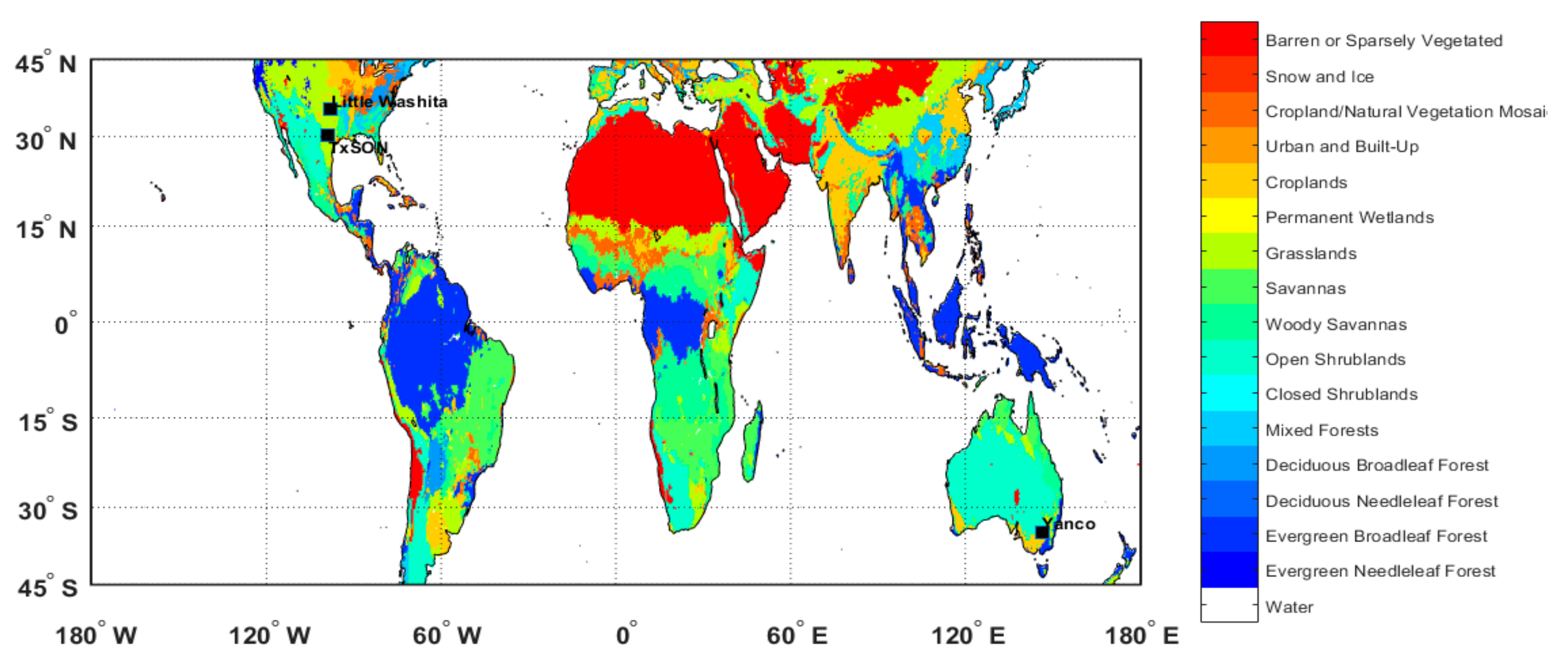
Figure 1 represents the International Geosphere-Biosphere Programme (IGBP) land classification, which arranged the type of Earth’s surface into 16 classes of land, including water. The IGBP is created by using Moderate Resolution Imaging Spectroradiometer (MODIS) data and it is included in SMAP metadata with equivalent resolution to soil moisture. Among the 16 classes of the land, the land cover classification of “grasslands” is used in the analysis process. As an initial study for calculating quantitative dielectric constant using GNSS-R, this research has only considered the reflection occurring on flat surfaces with grasslands. Some researchers have reported the results of the relationship between land classification and the qualities of the reflected signals from GNSS satellites [33,34,35]. In relation to this study, the quantitative effect of land classification to soil moisture will be the subject of a future study.
2.2. Data
As described, there have been numerous remote sensing satellite missions for measuring and monitoring soil moisture around the world. This paper focuses on data sets derived from two recent missions: SMAP and CYGNSS. The SMAP satellite was launched on 31 January 2015 with the objective of producing global soil moisture mapping and landscape freeze/thaw state via the L-band radar and radiometer employed [36]. The radiometer observes microwave emissions from the Earth’s surface through a 6 m antenna, measuring both vertical and horizon polarization. The observation results are provided by four levels of data product with various special resolutions being derived by the scientific objective for each level and available to access through the Alaska Satellite Facility (ASF) and the National Snow and Ice Data Center (NSIDC) website [37]. This research uses Level 3 version 6 soil moisture data with 36 km × 36 km spatial resolution being drawn on same distance of geophysical latitude and longitude, called the Equal-Area Scalable Grid (EASE-Grid) [38]. Additionally, a quality flag indicating the condition of the data accompanying SMAP metadata is used to acquire qualified and validated dielectric constant. The detailed process can be found in Section 4.
CYGNSS performing GNSS-R technology consists of eight nanosatellites for observing wind speed over the Earth’s tropical oceans to understand and predict the characteristics of hurricanes. The satellites were launched on 15 December 2016, orbiting an equatorial region with an inclination of 35°, 514 km perigee, and 536 km apogee. Each satellite’s orbit limits the instrument surface coverage to a latitude range of ±38°. The observations from each satellite have been made available by the Physical Oceanography Distributed Active Archive Center (PODAAC) (https://podaac.jpl.nasa.gov (accessed on 15 May 2021)) [39] since March 2017.
Each CYGNSS satellite contains a Delay Doppler Mapping Instrument (DDMI), which measures both the direct GPS signals and the GPS signals that are reflected from Earth’s surface. The DDMI can process up to four reflections simultaneously. The antenna on each satellite is capable of sensing the Right Hand Circular Polarization (RHCP) signals in the zenith direction and the Left Hand Circular Polarization (LHCP) signals in the nadir direction for the GPS L1 frequency. The observed signals are compressed and downloaded to the ground station, and then a post-processing procedure is applied to generate scientific observables satisfying the mission objective.
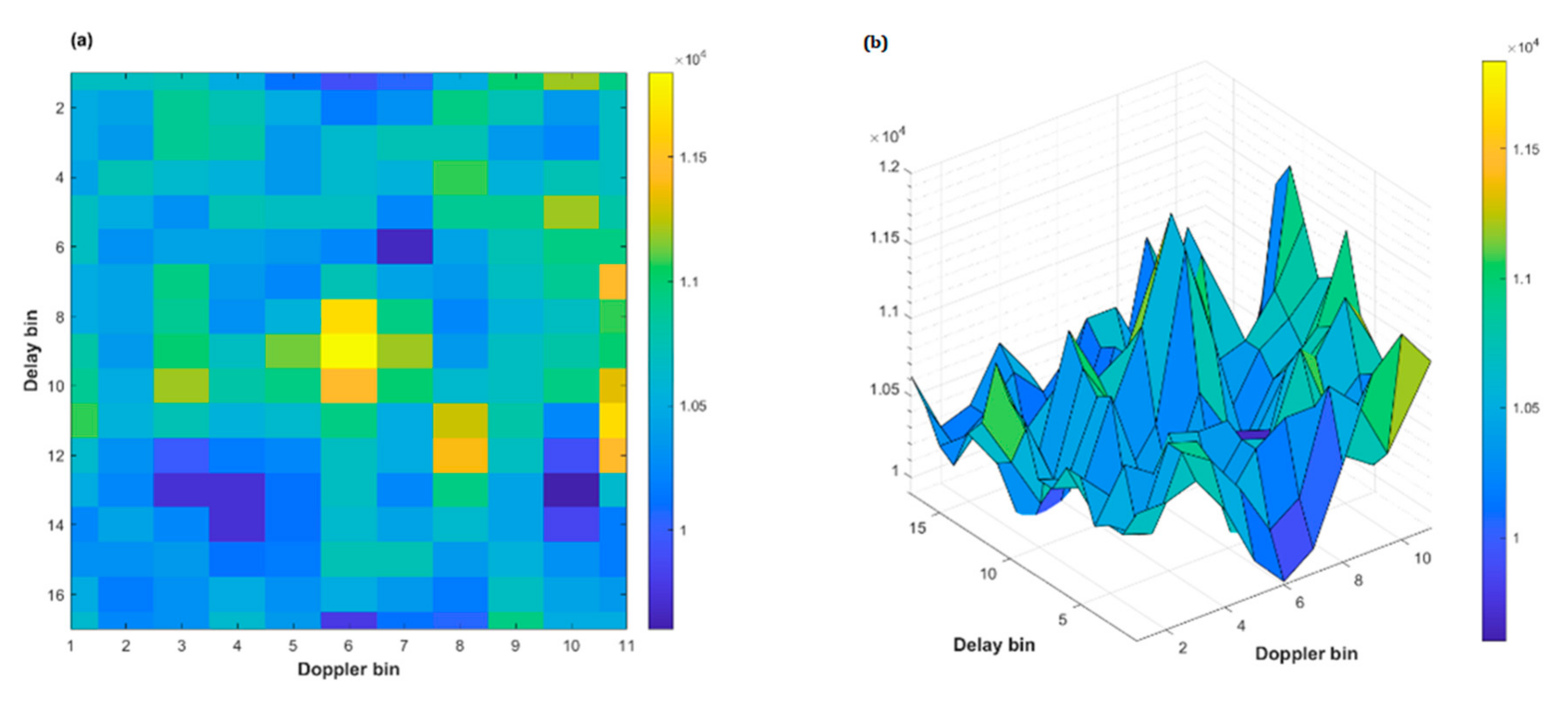
There are three accessible data levels published for the community. Level 1 (L1), version 2.1 data are used for the quantitative dielectric constant analysis in this study. Each observation file contains a number of observables and metadata, including Delay Doppler Maps (DDM—scattered power from specular point), as well as geometry information arranged by GPS satellite as transmitter, receiver, and specular power stored in daily NetCDF files. Detailed specifications and processing schemes can be found in [40]. The DDM is the fundamental product that is related to scattering physics affected by scattering geometry and conditions; this information is essential in progressing the analysis of GNSS-R data. Figure 2 provides a DDM example using CYGNSS data from 1 January 2019. CYGNSS data have been used for a variety of geophysical research, because the provided metadata include reflection geometry. The GNSS-R bistatic configurability differs from other active/passive remote sensing instruments, allowing for high surface spatial resolution. The first Fresnel zone or first glistening zone is regarded as the reflection zone for obtaining spatial resolution for a GNSS-R instrument. For example, in [41], the author evaluates that the spatial resolution of a CYGNSS signal, indicating the first Fresnel reflection zone, is approximately . However, it is still challenging to specify a definitive reflection region to produce authentic spatial resolution.
3. Methodology
This section presents the equations used in the data process as well as grid information to draw a 2D global image in analysis. The equations are composed of a reflection equation from electromagnetic theory combined with coherent radar equation. Computation results are drawn as 2D images using EASE grid v2.0, which have same distance in the latitudinal and longitudinal directions.
3.1. Analysis Method
According to conditions, such as surface roughness, incident angle, and vegetation type, GNSS signals experience two types of reflections: coherent scattering with identical incident and reflection angles; and, incoherent scattering, which has randomly distributed reflection angles. The scattering type can be determined by the maximum value and shape and magnitude of values around the maximum value in the DDM, as shown in Figure 2 and described in [13]. Theoretically, coherent scattering corresponds to a sharp peak in the DDM, because it has less obstacles for disrupting the original signal. An incoherent signal can be shown broadening around the maximum value as compared to signals from coherent scattering. Because a GNSS satellite broadcasts at the microwave frequency, both of the scattering signals are measured simultaneously by a nadir antenna.
The measured signal power, , from the nadir antenna can simply be expressed as the summation of coherent scattering and incoherent scattering , as in Equation 1.
In recent research, it is reported that the presence of an inland water body is associated with coherent reflection over land according to the spaceborne motivated observation and the extracting method developed for coherent scattering signals from an observed DDM by applying the Woodward ambiguity function [42]. Nevertheless, a restricted incident angle approach is used in this analysis to make the analysis process less complicated. As mentioned previously, higher incident angles have large opportunities for observing coherent scattering signals, given the concept that a small incident angle will increase the signal-to-noise ratio at the receiver and be applicable for neglecting coherent scattered signals from GNSS satellites. It was shown by [43] that the incident angles of less than 35° are able to represent the coherent scattering; thus, incident angles less than 20° from CYGNSS data are applied in this computation. The incident angle of 20° presenting the most correlated results has been selected to apply the computation progress in this analysis.
Equation (2) describes the coherent scattering equation, which is used to calculate the reflectivity Γ using the bi-static geometry of GNSS-R with coherent scattered signal power from the DDM [44].
Where is the peak value of DDM scattered power that is calculated from the raw count in CYGNSS data; N denotes the noise floor; and are the distant of transmitter and receiver from specular point, respectively; is the transmitter equivalent isotopically radiated power (EIRP); and, represents the receiver antenna gain in the direction of the specular point. In addition, the subscript ‘lr’ on the left-hand side expresses the polarization of incident signals and reflected signals, and r and t on the right-hand side indicate the reflected signals and direct signals, respectively. All of the variables are obtained from the v2.1 Level 1 CYGNSS product, as denoted.
The Fresnel coefficient, , is another important parameter in this analysis is that describes the reflection and transmission of electromagnetic radiation when an incident on an interface between different media occurs. The Fresnel coefficient connects the observable reflectivity and surface parameter, such as roughness and vegetations, and it is employed to convert the circular polarization properties of GNSS signals into linear polarization waves, which are generally adopted in electromagnetic reflection theory.
Equation (3) expresses the relation between the reflectivity and Fresnel coefficient as a function of wave number k, surface roughness σ, and elevation angle . The surface roughness is derived from the Shuttle Radar Topography Mission (SRTM) Digital Elevation Model (DEM) [45], and the wave number and incident angle are obtained from Level 1 CYGNSS data.
It is noted that the current electromagnetic scattering theory explains the natural phenomena with linear polarization waves; however, this circumstance exposes the necessity of expanding scattering theory in terms of circular polarization waves to infer accurate geophysical properties while using reflected GNSS signals. The Fresnel coefficient of circularly polarized waves being expressed as a linear combination of horizontal, h, and vertical, v was discussed by [46]. Fresnel coefficients use the transformation matrix shown in Equation (4):
The subscripts on both sides of Equation (4) represent the change in the wave polarization from the latter to the former subscript. For example, rl represents that the left-hand circular polarization wave changed to right-hand circular polarization. The linear polarized Fresnel coefficient of the horizontal and vertical direction can be expressed as Equation (5) [47]:
where is the signal incident angle and denotes the dielectric constant, which implies an electrical property of insulating material—a dielectric. The constant is the main parameter that is used to infer soil moisture using GNSS-R. With the inverted Fresnel equation for horizontal polarization, the dielectric constant can be simply expressed as Equation (6) in terms of the surface reflectivity and incident angle, as derived in [48]:
For CYGNSS data, the dielectric constant is computed using Equation (6) and it accumulated on the EASE grid. The detail process will be addressed in the following section.
3.2. EASE Grid 2.0
Spatial mismatch is the most common problem when the CYGNSS product is compared with SMAP satellite data. When compared to 2D images with the 36 km × 36 km spatial resolution from the SMAP product, CYGNSS data are provided with a list of tables containing post-processed results that are a sequence of observation results and metadata regarding orbit and satellite information. We applied the averaging method that was used in [12] to overcome the spatial resolution mismatch in comparing CYGNSS and SMAP reflectivity and dielectric constant. For this reason, CYGNSS reflectivity data on each EASE are located in the same grid of SMAP data. The EASE grid is defined as a global scale of gridding with the use of an equal area projection. Because the resolution of the EASE grid is varies depending on usage, the SMAP data provide soil moisture and other variables with varying spatial resolution, such as 3 km, 9 km, or 36 km. V2.0 denotes the updated method for reducing the spatial distortion when the projection is applied.
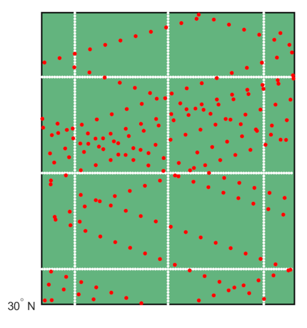
Figure 3 illustrates the orbit of CYGNSS satellites when one of eight satellites passes above the site TxSON in the United States. The white straight lines depict the EASE grid border and red dots represent the specular points that are measured by a CYGNSS satellite. The selected locations for analysis can be converted from geographic coordinates into the EASE grid using the conversion function shown in [49]. Subsequently, 2D images can be drawn by removing the average from the reflectivities belonging to same EASE grid of SMAP. When the average is applied, the time interval for the average is one day, and the data from eight satellites are used simultaneously without distinction. It is assumed that every satellite has identical measurement properties when they are measured by the reflected signals over the land. The assumption is caused by the fact that a specialized calibration process was not created for the measurement data from individual satellites. The calibration method for land-reflected GNSS signals will be specified by future work, and the soil moisture and dielectric constant values that are derived from GNSS-R observations will become more accurate.
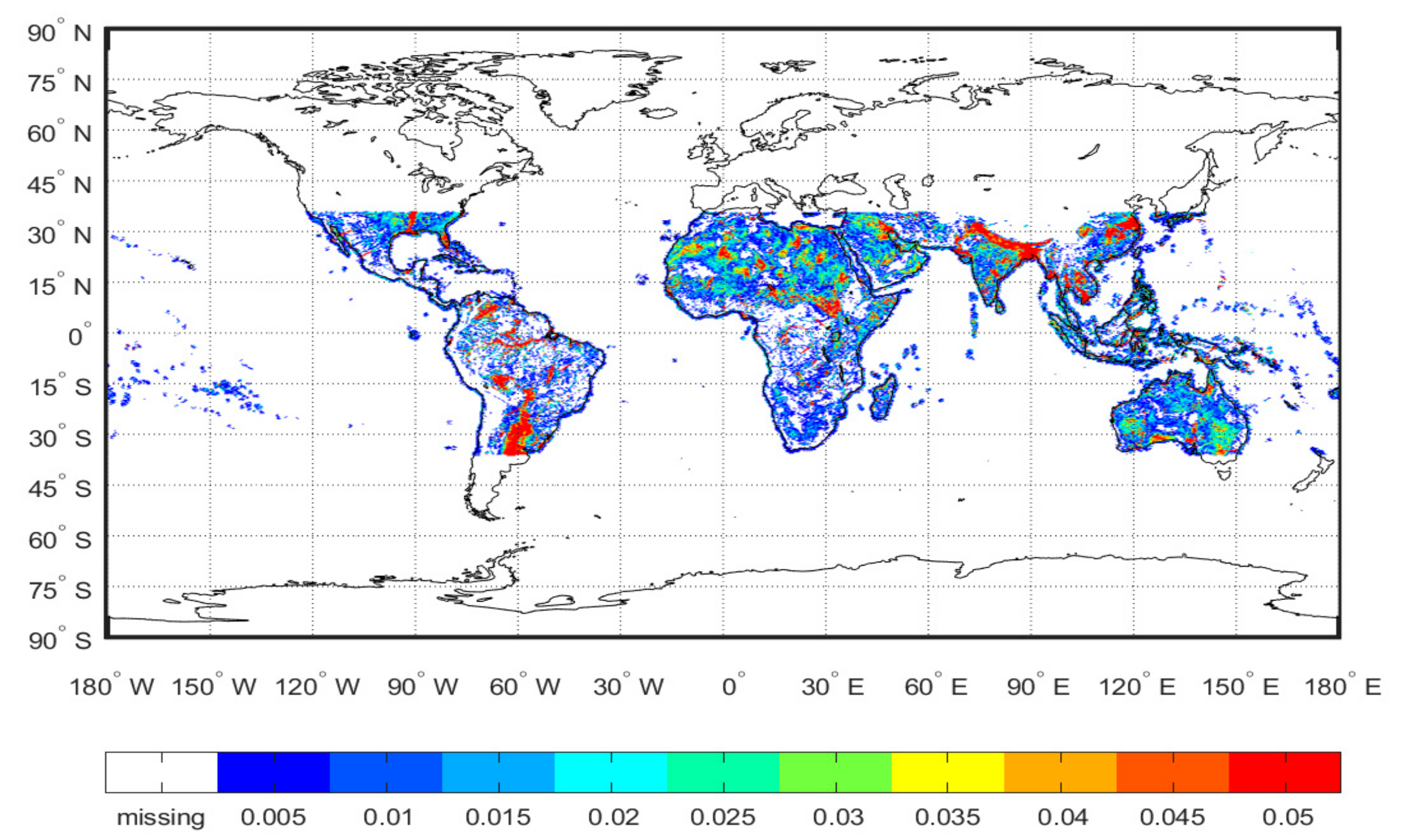
The averaged 2D global image of reflectivity using CYGNSS data can be obtained every day; then, by iterating the same process with another date of observation, a global number reflectivity is acquired. Figure 4 shows the global reflectivity map that was calculated with CYGNSS data using Equations (2) through (6) on the EASE grid v2.0 and accumulated observation data of satellite 1 from 18 March 2017 to 28 February 2018. Despite the low spatial resolution that is given by the 36 km × 36 km EASE grid, this method simplifies the comparison between CYGNSS and SMAP data. Additionally, it is a straightforward approach for applying the same process to other locations by changing the target pixel of analysis. As noted earlier, the data with incident angle greater than 20° have been removed in CYGNSS data. Iterated results at diverse locales are given in the following sections. The data correlation time series and seasonal variations will be examined in order to determine the time related properties.
4. Results
Following the analysis approach that is described in the previous section, the daily variation of dielectric constant from CYGNSS has been examined and compared with the SMAP data. The calculation and comparison processes are applied to three locations in the grass field category. The characteristics of dielectric constant along with the change of the season are also explored by comparing with the reference SMAP datasets.
4.1. Daily Time Variation of Dielectric Constant
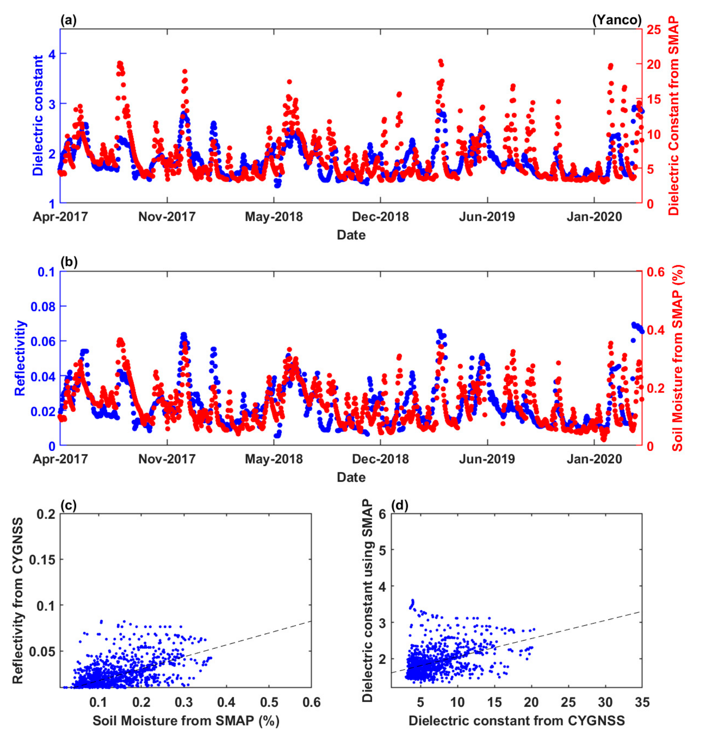
A typical feature of the derived dielectric constant using CYGNSS data along with daytime interval is investigated at distinct locations that were selected from the list of core validation sites for SMAP soil moisture. Figure 5 shows the time series comparisons and correlation scatter plots between CYGNSS and SMAP data when specular points occur at Yanco, Australia. The methods for drawing a 2D global image with EASE grid are applied to CYGNSS data, as explained in Section 3. Subsequently, the search process is applied to find the location of the pixel containing the geographical position of Yanco. Because the global soil moisture map from SMAP has been built on an EASE grid, the location of the pixel in CYGNSS 2D global map is identical to the SMAP global image. Analysis data observed on the desired specular point are extracted from the specific pixel in the 2D global map using CYGNSS and SMAP data. By repeating the described process to the entire satellite dataset, a daily time series figure can be obtained, as seen in Figure 5, Figure 6 and Figure 7. Approximately three years of CYGNSS and SMAP data were examined, spanning from March 2017 to April 2020. In Figure 5a,b, blue dots represent the dielectric constant and reflectivity from CYGNSS satellites and red dots indicate the soil moisture and dielectric constant that originated from the SMAP satellite. Figure 5a demonstrates the results of the dielectric constant derived from Equations (2) through (6) from CYGNSS data as compared with the dielectric constant calculated from the semi-empirical model that was applied to SMAP data. Figure 5b presents the comparison plot between reflectivity from Equation (2) with CYGNSS data and SMAP soil moisture data.
The CYGNSS-based estimation has the tendency of clearly following a SMAP-based dielectric constant and soil moisture, as seen in both Figure 5a,b. The computed dielectric constant and reflectivity results are also within the expected values: the dielectric constant is larger than 1 and the reflectivity is between 0 and 1, with no shifting of the data axis or normalization method applied to the CYGNSS data. These results are encouraging, as, at 6.6 times less the cost, the CYGNSS mission can provide soil moisture estimates that are comparable to those of the SMAP mission. Additionally, these correlations support quantitative values of soil moisture from CYGNSS satellites, because the dielectric constant, which plays an important role to calculate soil moisture, exists in a reasonable range when the GNSS-R data are applied. The difference of peak values between CYGNSS and SMAP can be observed in both Figure 5a,b. The peak values of dielectric constant presented in Figure 5a are shown to be distinct, and they are considered to have relations to weather condition, season, surface roughness, and, mostly, the calibration process. A more detailed comparison between the dielectric constant from CYGNSS and SMAP with the GNSS-R specified soil moisture model is an important part of future research.
Figure 5c,d demonstrate the statistical results by plotting the scattering features using the results presented in Figure 5a,b: Figure 5c shows the scattering plot using the reflectivity from CYGNSS and soil moisture from SMAP; Figure 5d is used to determine the correlation between the dielectric constant from CYGNSS and SMAP. The Root Mean Square Error (RMSE) and unbiased RMSE (ubRMSE) are used to capture the degree of correspondence between the estimated values and reference values [36], as well as to verify the developed method in the correlation plots. Figure 5a presents an RMSE of 5.73, while Figure 5b depicts a much lower RMSE of 0.13. The RMSE value using reflectivity and soil moisture is reasonable, since it is comparable to the results shown in previous research [12], and the RMSE of the dielectric constant has not been investigated in the published GNSS-R research. These results indicate that: (i) the dielectric constant obtained from GNSS-R using the devised method has greater equivalence than reflectivity as a function of soil moisture from the SMAP results; (ii) the calculated dielectric constant is estimated well with CYGNSS data; and, (iii) it is possible to quantitatively produce a dielectric constant using GNSS-R measurements.
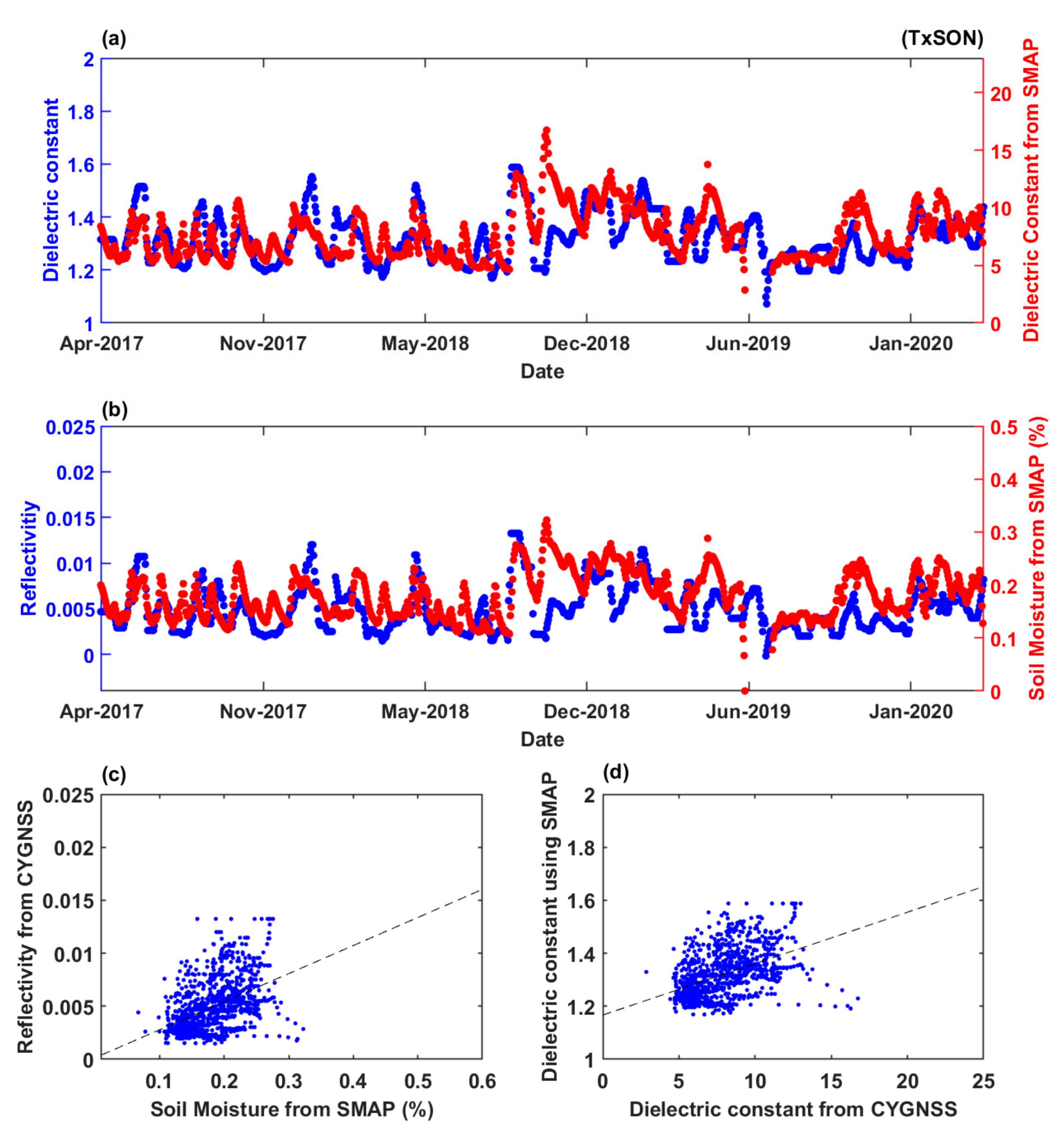
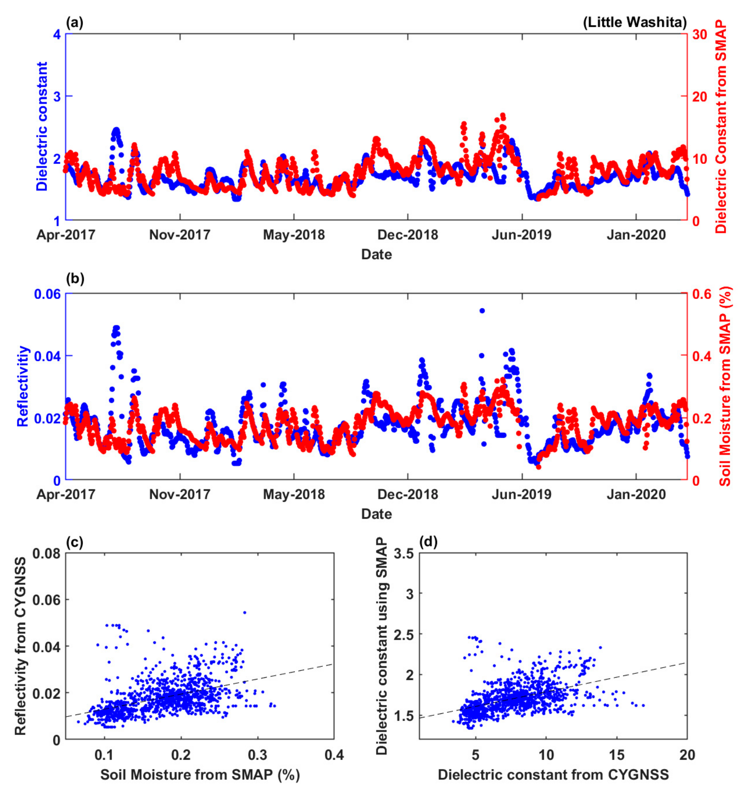
Figure 6 and Figure 7 illustrate additional comparison results between CYGNSS and SMAP satellite data that were measured at two other locations with substantially different environments. The observation results from TxSON, Texas, and Little Washita, Oklahoma in the U.S. have been investigated, and the equivalent analysis was performed as in Figure 5. As seen in Figure 6 and Figure 7, the computed dielectric constant and reflectivity results using CYGNSS data have comparable results with the dielectric constant and soil moisture from SMAP. The RMSE from the dielectric constant results is 6.65 at TxSON and 6.40 at Little Washita, which show comparable, but minimally distinct results from Yanco. This implies that computing the dielectric constant using GNSS-R is required for considering regional characteristics, such as roughness, topography, season, weather, etc. Seasonal variation is investigated in the following section and the topographic effects are analyzed by [50]; yet, the more combined analysis of the regional characteristics is necessary for obtaining precise dielectric constant and soil moisture using GNSS-R.
Table 1 lists additional results of confirmation metric, including unbiased RMSE for the three sets of analyses. The ubRMSE values are also calculated to remove the possible biases incurred in either mean or amplitude fluctuations in the retrieval process [36], and the data for calculating RMSE for the first and ubRMSE for the third row in the table are used in the computation. The second row represents the RMSE calculation and the fourth row depicts the ubRMSE computation that were used for data when Figure 5, Figure 6, and Figure 7b are drawn. The results indicate that the dielectric constants observed at the three different locations are similar to the SMAP results, as confirmed by the statistical analysis, and, when biases are reduced, the GNSS-R estimated dielectric constant is even more similar to the observation results from SMAP. The Pearson correlation coefficient is also calculated and evaluated for the three analysis locations. Two correlation coefficients show positive correlation, and they are comparable with each other, similar to RMSE and ubRMSE, as seen in Table 1. The results indicate that the correlation coefficient results also support the compatibility of the computation approach to compute the dielectric constant using the GNSS reflectometry instrument. On the other hand, it will also arise in future analysis when considering the regional characteristics.
Therefore, it can be concluded that the developed method for calculating the dielectric constant using CYGNSS data produces a consistent dielectric constant that corresponds to satellite-based references, especially when the specular point occurs on flat and grass field areas. Future work will determine the dielectric constant that is measured at locations other than core validation sites, and distinct land classifications will be explored. Investigations of other locations or vegetation will also be instructive in finding out the characteristics of the dielectric constant or soil moisture according to topography, as per [50].
4.2. Seasonal Variation at Various Locations
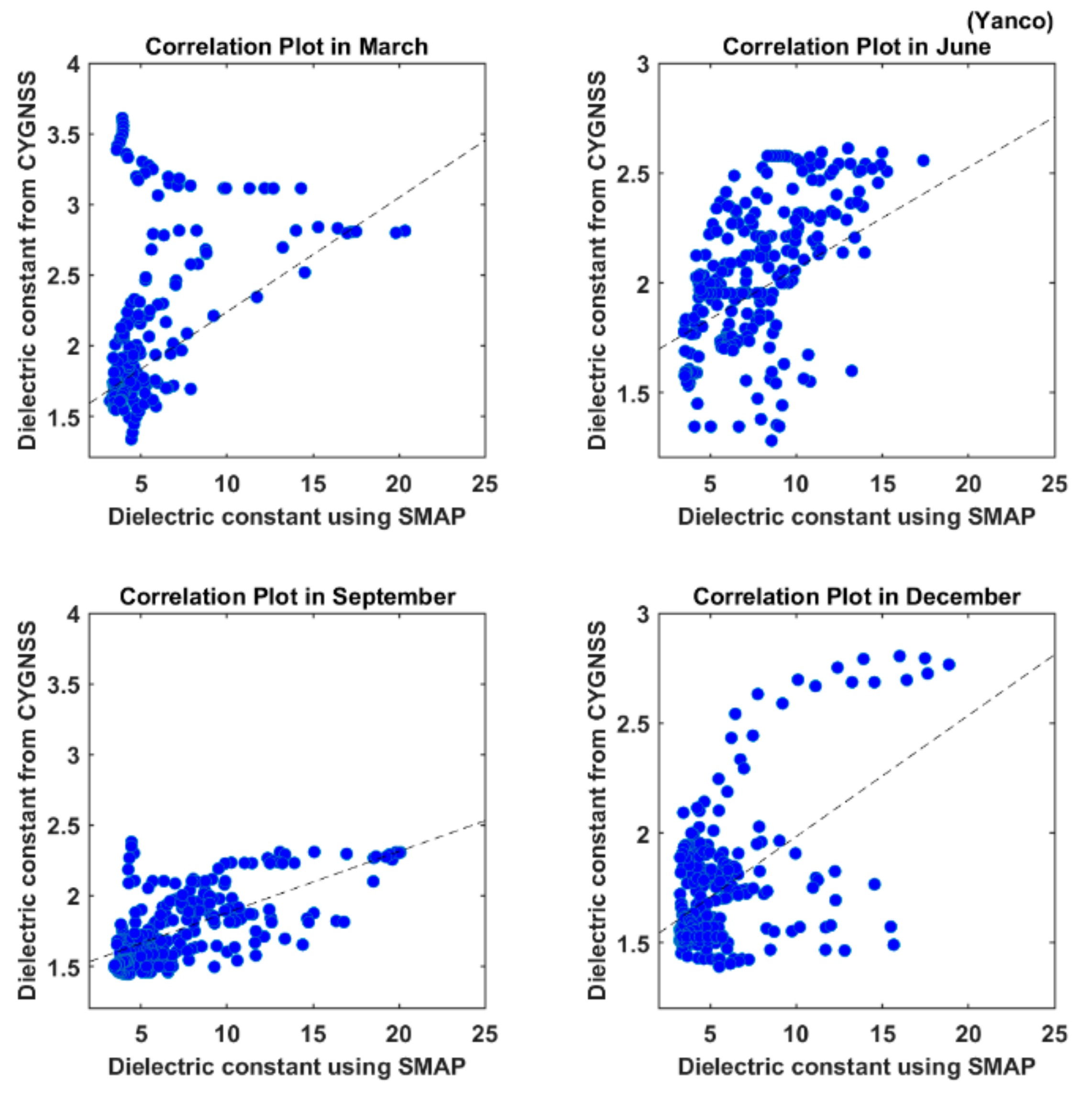
The seasonal variations of the derived dielectric constant are examined in this section, which is necessary for speculating how adequately the dielectric constants are estimated by using reflected GNSS signals. This analysis is used to understand the effect of the environmental change on dielectric constant, as well as vegetation effects. Figure 8 through 10 illustrate the scattering plots separated by the four seasons. The dielectric constants used in analysis are calculated from CYGNSS and SMAP exactly as per the previous section. Each dataset is separated into four seasons: March Equinox, June Solstice, September Equinox, and December Solstice while following the described sequence: (1) determine the Solstice and Equinox dates in each year; (2) gather data from 45 days prior to 45 days after each Solstice/Equinox; (3) apply the data collection process to other years of data; (4) merge the yearly separated data to one variable according to the Solstice and Equinox event; and, finally, (5) draw correlation plots in terms of each season. The entire separation process is repeated for the same core SMAP validation sites: Yanco, TxSON, and Little Washita.
Additionally, it is noted that SMAP Level 3 products are not available from mid-June 2019 to the end of July 2019. On the evening of 19 June 2019, the SMAP satellite turned into safe mode, which is a state of shutting down all instruments and, therefore, data collection was disrupted. After several recovery attempts, SMAP returned to science mode and resumed science data collection on 23 July 2019 [51]. With this absence of observations, the analysis results in June for every seasonal plot will be statistically insufficient and, therefore, cause errors.
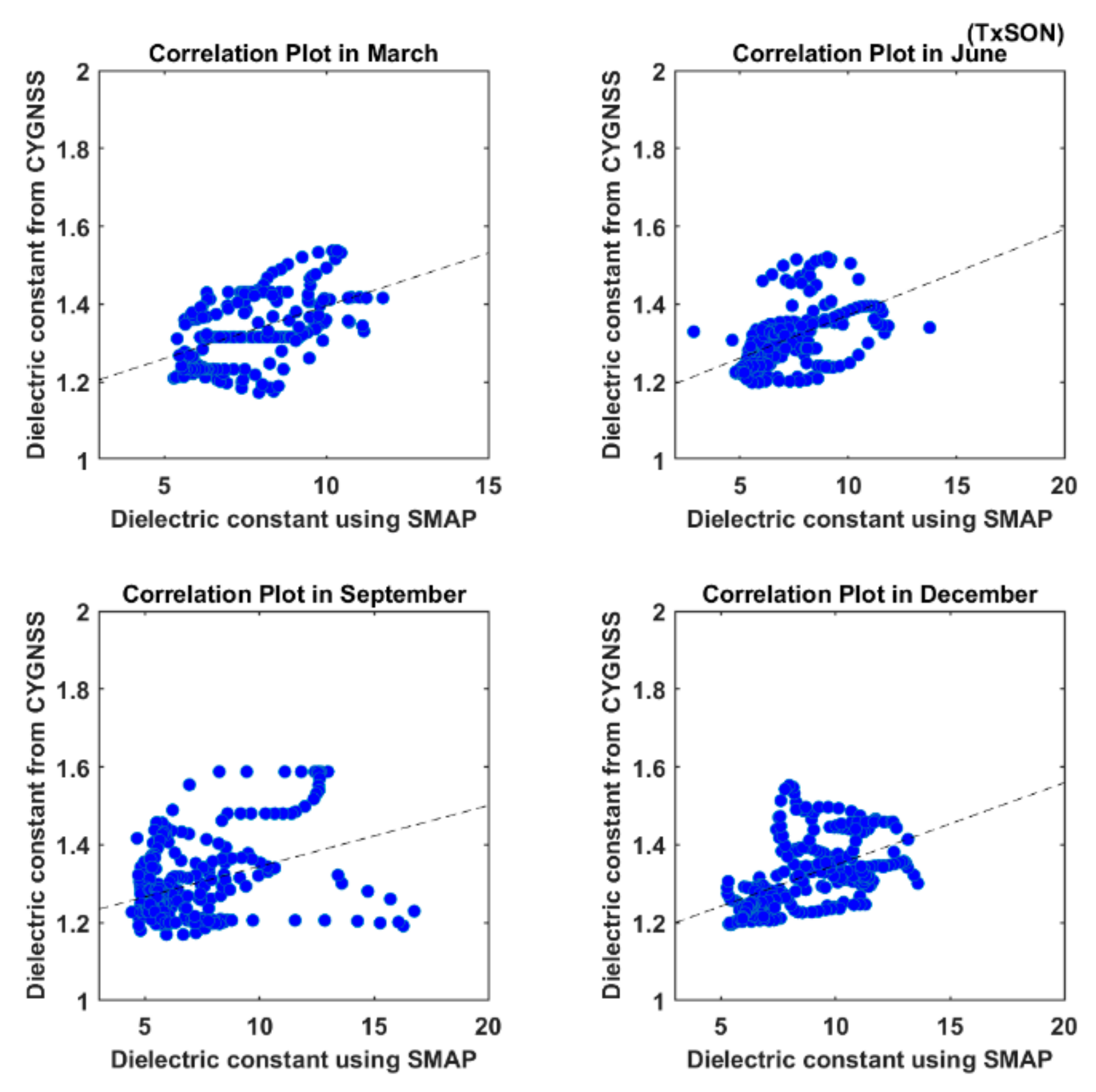
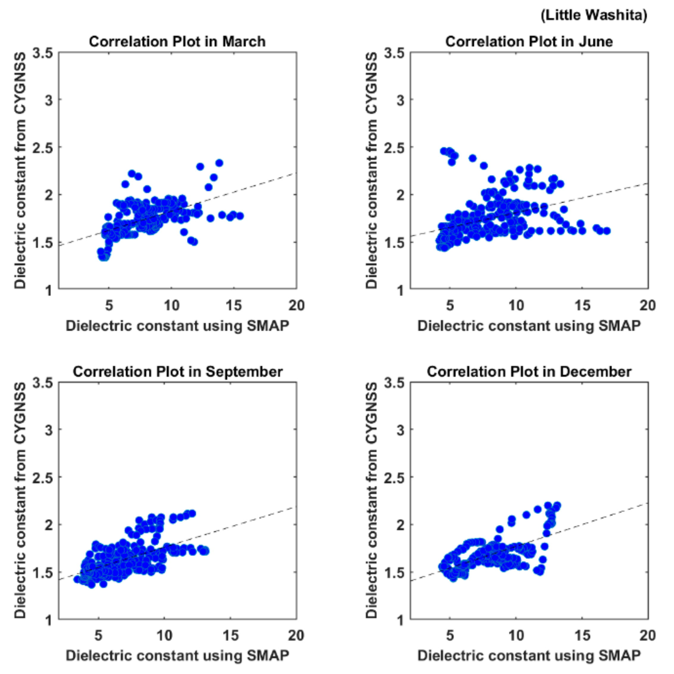
The dielectric constant that is determined from CYGNSS is correlated with dielectric constant from SMAP in every season, as shown in Figure 8 through 10. RMSE has been calculated for every season in order to evaluate the variance of the derived dielectric constant when compared with this reference. Table 2 lists the results of RMSE, ubRMSE, and correlation coefficient statistics using the dielectric constant measured at Yanco, TxSON, and Little Washita. The equivalent data used to draw Figure 8, Figure 9 and Figure 10 are adapted to calculate Table 2.
The results shown in Table 2 indicate that each confirmation parameter is comparable with the value calculated using the entire duration of data. In addition, the confirmation results show that the relevant variation depends on the season, but the factors causing seasonal variation require identification by further investigation. Even though the eight CYGNSS satellites cover the tropical region of the Earth, the specular points are sparsely distributed on the EASE grid, because a single observation using reflected GPS L1 signals will span approximately four months to cover the entire Earth. Thus, by adding more satellites or implementing a multi-GNSS constellation receiver, observing not only GPS L1, but also signal transmitted from GLONASS, Galileo, and Beidou, may allow for reliable determination of seasonal variation.
5. Discussion
Dielectric constant, which is a crucial indicator for soil moisture retrieval, has been estimated using the products from a GNSS-R instrument, specifically from the CYGNSS satellite constellation mission. In this study, sequential and seasonal variations of dielectric constant have been evaluated using the method, as described in [43]. The dielectric constant has been validated by the comparisons of the reference data to the SMAP satellite-derived soil moisture, and it has been statistically quantified by low values of confirmation metrics. A few subjects are addressed in this section in order to identify the parameters that influence the determination of dielectric constant from GNSS-R and soil moisture. Each topic is required to be analyzed further in order to anticipate the quantitative soil moisture content determination using GNSS-R data.
- Vegetation type or land classification: the classification of land can be of concern due to the parameters that affect the calculation of dielectric constant when the reflectivity is transformed to the Fresnel reflection coefficient (Equation (3)). Therefore, an investigation, including vegetation type, is essential for improving the qualities of soil moisture or dielectric constant retrieval. Over the past few decades, there has been an attempt to classify land type by observing topography using satellite instruments, such as the International Geosphere–Biosphere Programme (IGBP) Land Classification. With comprehensive analysis regarding reflections over distinct land classifications, the results from GNSS-R will be similar to the reference instrument. NDVI or Freeze/thaw state will also be related to the dielectric constant, as referred to in [52]. Elaborated analysis for figuring out the characteristics of derived dielectric constant will be done in future research.
- Spatial resolution: in this research, the EASE grid v2.0 with 36 km × 36 km of resolution is applied to build two-dimensional images and to acquire information from assigned pixels according to specified locations. From the perspective of global images, the 36 km resolution is good enough to produce usable imagery. The land surface and other classifications, such as urban, cropland, or grassland, were included in the designated pixel. In other words, two specular points in the same pixel are possible for experiencing the reflection on different land classifications. Because the averaging of data over the same pixel has been implemented, the resulting dielectric constant estimates must contain an error. Increasing spatial resolution and investigating land classification is required to remove errors. However, the specific approach is demanding, because high spatial resolution can cause statistical errors for short periods of observations.
- Soil moisture model: a soil moisture model was applied to convert soil moisture from SMAP to the dielectric constant. In this conversion, the semi-empirical model is used [29]; although, the semi-empirical model was developed based on the in-situ measurements of microwave frequency waves rather than a remote sensing technique. Because the semi-empirical soil moisture model is not specialized to GNSS-R, it consistently contains unexpected errors in conversion. Even though it was established to deal with remote sensing observation results, it still required particular soil moisture to produce coincident results while using GNSS-R.
6. Conclusions
A procedure for calculating dielectric constant using GNSS-R has been tested with data from the CYGNSS satellites. Version 2.1 CYGNSS data were used for the computation method, and Level 3 SMAP soil moisture data with 36 km × 36 km were used as a reference to validate the calculation results. A restriction of incident angle was applied in order to extract coherent scattering components from combined signals that were captured by the LHCP antenna on each CYGNSS satellite. A multi-step mathematical approach has been implemented for approximately three years of data with the objective of synthesizing calculation process to acquire dielectric constant. Reflectivity, which is the ratio of GNSS signal captured by the zenith direction antenna and nadir direction antenna, from the CYGNSS data is converted to Fresnel reflection coefficient with surface roughness information from SRTM. The Fresnel reflection coefficient was applied through the use of an equation developed to derive dielectric constant from radiometer observations. The spatial resolution of CYGNSS data was adjusted on the EASE grid v2.0 coordinates for drawing a 2D global image. The derived dielectric constant has been validated with soil moisture, and the dielectric constant was converted by the semi-empirical soil moisture model. The dielectric constant that was retrieved from CYGNSS data shows values ranging between 1 to 3; whereas, the dielectric constant retrieved from SMAP data shows values that ranged from approximately 5 to 20. Both of the dynamic ranges have different values with a range from 2 to 16 for the dielectric constant retrieved from reflected GPS signals, as presented by [16]. The dynamic range difference is potentially caused by the simplified model that is used to understand the link between land geophysical parameters, because the dielectric constant is dependent on different soil characteristics (soil moisture, soil salinity content, soil type, and/or temperature).
In addition, it is understood that the dielectric constant should not be influenced by changing the observation instruments as well as retrieval models. Nevertheless, selecting the correct mathematical model is important in data analysis, especially in GNSS reflectometry, during the calculation of the dielectric constant or soil moisture because an established retrieval model is based on specific experimental results. This research applied a mathematical model that was developed for handling radiometer data and used to calculate the dielectric constant. This retrieval model is useful for estimating dielectric constant, because it only requires the reflectivity results from the instruments, though it is inevitable to contain errors in the dynamic range, because the model is built to implement radiometer data. On the contrary, [16] used the Wang and Schmugge empirical model in computing the dielectric constant, which requires other parameters, such as frequency and temperature. Therefore, [16] represented the accurate dynamic range of the dielectric constant, even though this research produced significant results emphasizing a practical usage of GNSS Reflectometry instrument by only using the GNSS-R results and generating the dynamic range within the accurate dielectric constant range. In addition, the restriction of the incident angle in this analysis may affect the dielectric constant results, so needs to be further investigated.
Yanco, TxSON, and Little Washita were used in the analysis, which are core validation sites for verifying SMAP soil moisture data using in-situ measurement data. These reference sites were selected for the characteristics of flat and grass field in order to ignore the effect of roughness in the reflected GNSS signals and concentrate on the computation process for dielectric constant. The daily time series plots from these reference sites indicate that the analysis process can be regarded as consistent with other research, because the dielectric constant from CYGNSS corresponds to the dielectric constant that is converted from SMAP soil moisture using the semi-empirical soil moisture model. The confirmation metrics, RMSE, ubRMSE, and Pearson correlation coefficient were used to validate the dielectric constant results. It is reported that the RMSE and ubRMSE values using dielectric constants from CYGNSS and SMAP are 5.71 and 3.31, respectively, and the Pearson correlation coefficient is approximately 0.4 in the case of analysis on Yanco. The other two locations have comparable results in the confirmation metrics to the results at Yanco. It can be concluded that the multi-step mathematical approach is well established, and it is required to include vegetation and topographical analysis to acquire a precise dielectric constant from GNSS-R. A seasonal analysis was also performed, and shows the annual variation of the derived dielectric constant by comparing it to the SMAP data. The confirmation metrics for seasonal analysis are comparable to the time series results, but there was no correlated tendency among the different analysis sites. This result means that it is necessary to determine the parameters influencing the seasonal variation in soil moisture in future analysis. The types of vegetation, surface roughness, and spatial resolution are considered as variables for improving the accuracy of soil moisture retrieval using GNSS-R instruments. Using a distinct soil moisture model that is derived from GNSS-R observation rather than in-situ measurements is also required for acquiring a precise soil moisture model.
7. Future Work
In regard to future research in this field of study, the main concern in soil moisture retrieval will be to obtain quantitative soil moisture estimates from dielectric constant values and advanced research to determine more accurate dielectric constant. Researching the effect of land classification types on the dielectric constant can be achieved using analysis that is similar to that used in this study. In addition, the separation of coherent and incoherent scattering components in delayed Doppler maps is a challenging domain of research due to the combination of electromagnetic scattering theory and data analysis. Regardless of the difficulty, the separation of scattering components will contribute to not only GNSS reflectometry, but also electromagnetic theory. Moreover, the results of this work will maximize the benefit of a GNSS-R instrument by investigating the effect of incident angle on scattering. Observing RHCP reflected GNSS signals in the nadir direction will also require accurate dielectric constant values.
The GNSS Lab at York University, Canada, is developing a Field Programmable Gate Array (FPGA)-based GNSS-R receiver, which is funded by the Canadian Space Agency. Its general objective is to teach students to develop their knowledge of space. Its scientific objective is to estimate the soil moisture content onboard various platforms and it is scheduled to be flown on an unmanned aerial vehicle (UAV) and an aircraft. With these experimental experiences, the GNSS Lab will be designing and developing a receiver for use on a nanosatellite in low Earth orbit. At present, a prototype GNSS-R receiver has been built using commercial off-the-shelf parts. Outdoor testing will be conducted over longer periods, and across various soil types, vegetation, and topography. The results from this GNSS-R receiver will contribute to organizing the calibration method for the instrument on land surfaces and local soil moisture modelling. It is then expected that this process will provide quantitative soil moisture data, not only for local regions, but also global places, and will induce positive interactions with various fields, such as climate research and the agricultural industry.
Author Contributions
Conceptualization, J.L.; Data curation, N.G.K.; Investigation, J.L.; Methodology, J.L.; Project administration, S.B.; Resources, S.B.; Supervision, S.B. and R.S.K.L.; Validation, J.L. and N.G.K.; Visualization, J.L.; Writing—original draft, J.L.; Writing—review & editing, S.B., R.S.K.L. and N.G.K. All authors have read and agreed to the published version of the manuscript.
Funding
This research was funded by Canadian Space Agency (CSA), grant number 18FAYORA09.
Data Availability Statement
The data presented in this study are openly available in PO.DAAC, reference number [39].
Acknowledgments
This work is supported by the Canadian Space Agency’s Flights and Fieldwork for the Advancement of Science and Technology (FAST) funding program.
Conflicts of Interest
The authors declare no conflict of interest.
References
- Lakshmi, V. Remote Sensing of Soil Moisture. ISRN Soil. Sci. 2013, 2013, 1–33. [Google Scholar] [CrossRef]
- Hollinger, J.P.; Peirce, J.L.; Poe, G.A. SSM/I Instrument Evaluation. IEEE Trans. Geosci. Remote Sens. 1990, 28, 781–790. [Google Scholar] [CrossRef]
- Paloscia, S.; Macelloni, G.; Santi, E.; Koike, T. A Multifrequency Algorithm for the Retrieval of Soil Moisture on a Large Scale Using Microwave Data from SMMR and SSM/I Satellites. IEEE Trans. Geosci. Remote Sens. 2019, 39, 1655–1661. [Google Scholar] [CrossRef]
- Guha, A.; Lakshmi, V. Sensitivity, Spatial Heterogeneity, and Scaling of C-Band Microwave Brightness Temperatures for Land Hydrology Studies. IEEE Trans. Geosci. Remote Sens. 2002, 40, 2626–2635. [Google Scholar] [CrossRef]
- Guha, A.; Lakshmi, V. Use of the Scanning Multichannel Microwave Radiometer (SMMR) to Retrieve Soil Moisture and Surface Temperature over the Central United States. IEEE Trans. Geosci. Remote Sens. 2004, 42, 1482–1494. [Google Scholar] [CrossRef]
- Ulaby, F.T.; Dubois, P.C.; van Zyl, J. Radar Mapping of Surface Soil Moisture. J. Hydrol. 1996, 184, 57–84. [Google Scholar] [CrossRef]
- Schmugge, T.J.; Kustas, W.P.; Ritchie, J.C.; Jackson, T.J.; Rango, A. Remote Sensing in Hydrology. Adv. Water Resour. 2002, 25, 1367–1385. [Google Scholar] [CrossRef]
- Martin-Neira, M. A Passive Reflectometry and Interferometry System (PARIS): Applications to Ocean Altimetry. ESA J. 1993, 17, 331–355. [Google Scholar]
- Garrison, J.L.; Komjathy, A.; Zavorotny, V.U.; Katzberg, S.J. Wind Speed Measurement Using Forward Scattered GPS Signals. IEEE Trans. Geosci. Remote Sens. 2002, 40, 50–65. [Google Scholar] [CrossRef] [Green Version]
- Zavorotny, V.U.; Voronovich, A.G. Scattering of GPS Signals from the Ocean with Wind Remote Sensing Application. IEEE Trans. Geosci. Remote Sens. 2000, 38, 951–964. [Google Scholar] [CrossRef] [Green Version]
- Cardellach, E.; Fabra, F.; Rius, A.; Pettinato, S.; D’Addio, S. Characterization of Dry-Snow Sub-Structure Using GNSS Reflected Signals. Remote Sens. Environ. 2012, 124, 122–134. [Google Scholar] [CrossRef]
- Chew, C.C.; Small, E.E. Soil Moisture Sensing Using Spaceborne GNSS Reflections: Comparison of CYGNSS Reflectivity to SMAP Soil Moisture. Geophys. Res. Lett. 2018, 45, 4049–4057. [Google Scholar] [CrossRef] [Green Version]
- Chew, C.; Shah, R.; Zuffada, C.; Hajj, G.; Masters, D.; Mannucci, A.J. Demonstrating Soil Moisture Remote Sensing with Observations from the UK TechDemoSat-1 Satellite Mission. Geophys. Res. Lett. 2016, 43, 3317–3324. [Google Scholar] [CrossRef] [Green Version]
- Camps, A.; Park, H.; Pablos, M.; Foti, G.; Gommenginger, C.P.; Liu, P.-W.; Judge, J. Sensitivity of GNSS-R Spaceborne Observations to Soil Moisture and Vegetation. IEEE J. Sel. Top. Appl. 2016, 9, 4730–4742. [Google Scholar] [CrossRef] [Green Version]
- Egido, A.; Paloscia, S.; Motte, E.; Guerriero, L.; Pierdicca, N.; Caparrini, M.; Santi, E.; Fontanelli, G.; Floury, N. Airborne GNSS-R Polarimetric Measurements for Soil Moisture and Above-Ground Biomass Estimation. IEEE J. Sel. Top. Appl. 2014, 7, 1522–1532. [Google Scholar] [CrossRef]
- Katzberg, S.J.; Torres, O.; Grant, M.S.; Masters, D. Utilizing Calibrated GPS Reflected Signals to Estimate Soil Reflectivity and Dielectric Constant: Results from SMEX02. Remote Sens. Environ. 2006, 100, 17–28. [Google Scholar] [CrossRef] [Green Version]
- Rodriguez-Alvarez, N.; Bosch-Lluis, X.; Camps, A.; Vall-llossera, M.; Valencia, E.; Marchan-Hernandez, J.F.; Ramos-Perez, I. Soil Moisture Retrieval Using GNSS-R Techniques: Experimental Results Over a Bare Soil Field. IEEE Trans. Geosci. Remote Sens. 2009, 47, 3616–3624. [Google Scholar] [CrossRef]
- Small, E.E.; Larson, K.M.; Chew, C.C.; Dong, J.; Ochsner, T.E. Validation of GPS-IR Soil Moisture Retrievals: Comparison of Different Algorithms to Remove Vegetation Effects. IEEE J. Sel. Top. Appl. 2016, 9, 4759–4770. [Google Scholar] [CrossRef]
- Clarizia, M.P.; Ruf, C.S. On the Spatial Resolution of GNSS Reflectometry. IEEE Geosci. Remote Sens. Lett. 2016, 13, 1064–1068. [Google Scholar] [CrossRef]
- Cardellach, E.; Rius, A.; Martin-Neira, M.; Fabra, F.; Nogues-Correig, O.; Ribo, S.; Kainulainen, J.; Camps, A.; D’Addio, S. Consolidating the Precision of Interferometric GNSS-R Ocean Altimetry Using Airborne Experimental Data. IEEE Trans. Geosci. Remote Sens. 2014, 52, 4992–5004. [Google Scholar] [CrossRef]
- Cardellach, E.; Li, W.; Rius, A.; Semmling, M.; Wickert, J.; Zus, F.; Ruf, C.S.; Buontempo, C. First Precise Spaceborne Sea Surface Altimetry with GNSS Reflected Signals. IEEE J. Sel. Top. Appl. 2019, 13, 102–112. [Google Scholar] [CrossRef]
- Zavorotny, V.U.; Voronovich, A.G. Bistatic GPS Signal Reflections at Various Polarizations from Rough Land Surface with Moisture Content. In Proceedings of the IEEE 2000 International Geoscience and Remote Sensing Symposium—Taking the Pulse of the Planet: The Role of Remote Sensing in Managing the Environment, Honolulu, HI, USA, 24–28 July 2000; Volume 7, pp. 2852–2854. [Google Scholar] [CrossRef]
- Rodriguez-Alvarez, N.; Camps, A.; Vall-Llossera, M.; Bosch-Lluis, X.; Monerris, A.; Ramos-Perez, I.; Valencia, E.; Marchan-Hernandez, J.F.; Martinez-Fernandez, J.; Baroncini-Turricchia, G.; et al. Land Geophysical Parameters Retrieval Using the Interference Pattern GNSS-R Technique. IEEE Trans. Geosci. Remote Sens. 2011, 49, 71–84. [Google Scholar] [CrossRef]
- Ruf, C.S.; Atlas, R.; Chang, P.S.; Clarizia, M.P.; Garrison, J.L.; Gleason, S.; Katzberg, S.J.; Jelenak, Z.; Johnson, J.T.; Majumdar, S.J.; et al. New Ocean Winds Satellite Mission to Probe Hurricanes and Tropical Convection. Bull. Am. Meteorol. Soc. 2016, 97, 385–395. [Google Scholar] [CrossRef]
- Kim, H.; Lakshmi, V. Use of Cyclone Global Navigation Satellite System (CyGNSS) Observations for Estimation of Soil Moisture. Geophys. Res. Lett. 2018, 45, 8272–8282. [Google Scholar] [CrossRef] [Green Version]
- Guo, P.; Shi, J.; Gao, B.; Wan, H. Evaluation of Errors Induced by Soil Dielectric Models for Soil Moisture Retrieval at L-Band. In Proceedings of the 2016 IEEE International Geoscience and Remote Sensing Symposium (IGARSS), Beijing, China, 10–15 July 2016; pp. 1679–1682. [Google Scholar] [CrossRef]
- Yang, T.; Wan, W.; Sun, Z.; Liu, B.; Li, S.; Chen, X. Comprehensive Evaluation of Using TechDemoSat-1 and CYGNSS Data to Estimate Soil Moisture over Mainland China. Remote Sens. 2020, 12, 1699. [Google Scholar] [CrossRef]
- Hallikainen, M.; Ulaby, F.; Dobson, M.; El-rayes, M.; Wu, L. Microwave Dielectric Behavior of Wet Soil-Part 1: Empirical Models and Experimental Observations. IEEE Trans. Geosci. Remote Sens. 1985, GE-23, 25–34. [Google Scholar] [CrossRef]
- Dobson, M.C.; Ulaby, F.T.; Hallikainen, M.T.; El-Rayes, M.A. Microwave Dielectric Behavior of Wet Soil-Part II: Dielectric Mixing Models. IEEE Trans. Geosci. Remote Sens. 1985, GE-23, 35–46. [Google Scholar] [CrossRef]
- Jia, Y.; Savi, P.; Canone, D.; Notarpietro, R. Estimation of Surface Characteristics Using GNSS LH-Reflected Signals: Land Versus Water. IEEE J. Sel. Top. Appl. 2016, 9, 4752–4758. [Google Scholar] [CrossRef]
- Egido, A.; Ruffini, G.; Caparrini, M.; Martin, C.; Farres, E.; Banque, X. Soil moisture monitorization using gnss reflected signals. arXiv 2008, arXiv:0805.1881. [Google Scholar]
- Colliander, A.; Jackson, T.J.; Bindlish, R.; Chan, S.; Das, N.; Kim, S.B.; Cosh, M.H.; Dunbar, R.S.; Dang, L.; Pashaian, L.; et al. Validation of SMAP Surface Soil Moisture Products with Core Validation Sites. Remote Sens. Environ. 2017, 191, 215–231. [Google Scholar] [CrossRef]
- Pierdicca, N.; Guerriero, L.; Giusto, R.; Brogioni, M.; Egido, A. SAVERS: A Simulator of GNSS Reflections from Bare and Vegetated Soils. IEEE Trans. Geosci. Remote Sens. 2014, 52, 6542–6554. [Google Scholar] [CrossRef]
- Small, E.E.; Larson, K.M.; Braun, J.J. Sensing Vegetation Growth with Reflected GPS Signals. Geophys. Res. Lett. 2010, 37, L12401. [Google Scholar] [CrossRef]
- Hu, C.; Benson, C.; Park, H.; Camps, A.; Qiao, L.; Rizos, C. Detecting Targets above the Earth’s Surface Using GNSS-R Delay Doppler Maps: Results from TDS-1. Remote Sens. 2019, 11, 2327. [Google Scholar] [CrossRef] [Green Version]
- Entekhabi, D.; Reichle, R.H.; Koster, R.D.; Crow, W.T. Performance Metrics for Soil Moisture Retrievals and Application Requirements. J. Hydrometeorol. 2010, 11, 832–840. [Google Scholar] [CrossRef]
- SMAP L3 Radiometer Global Daily 36 Km EASE-Grid Soil Moisture, Version 6. Available online: https://nsidc.org/data/SPL3SMP/versions/6 (accessed on 15 May 2021).
- O’Neill, P.E.; Chan, S.; Njoku, E.G.; Jackson, T.; Bindlish, R.; Chaubell, J. SMAP L3 Radiometer Global Daily 36 Km EASE-Grid Soil Moisture, Version 6. Available online: https://doi.org/10.5067/EVYDQ32FNWTH (accessed on 15 August 2019).
- PO.DAAC. Available online: https://podaac.jpl.nasa.gov/ (accessed on 14 May 2018).
- Ruf, C.; Chang, P.S.; Clarizia, M.-P.; Gleason, S.; Jelenak, Z.; Majumdar, S.; Morris, M.; Murray, J.; Musko, S.; Posselt, D.; et al. CYGNSS Handbook Cyclone Global Navigation Satellite System: Deriving Surface Wind Speeds in Tropical Cyclones; National Aeronautics and Space Administration: Ann Arbor, MI, USA, 2016; ISBN 978-1-60785-380-0.
- Chew, C.; Lowe, S.; Parazoo, N.; Esterhuizen, S.; Oveisgharan, S.; Podest, E.; Zuffada, C.; Freedman, A. SMAP Radar Receiver Measures Land Surface Freeze/Thaw State through Capture of Forward-Scattered L-Band Signals. Remote Sens. Environ. 2017, 198, 333–344. [Google Scholar] [CrossRef]
- Al-Khaldi, M.M.; Johnson, J.T.; O’Brien, A.J.; Balenzano, A.; Mattia, F. Time-Series Retrieval of Soil Moisture Using CYGNSS. IEEE Trans. Geosci. Remote Sens. 2019, 57, 4322–4331. [Google Scholar] [CrossRef]
- Calabia, A.; Molina, I.; Jin, S. Soil Moisture Content from GNSS Reflectometry Using Dielectric Permittivity from Fresnel Reflection Coefficients. Remote Sens. 2020, 12, 122. [Google Scholar] [CrossRef] [Green Version]
- Clarizia, M.P.; Pierdicca, N.; Costantini, F.; Floury, N. Analysis of CYGNSS Data for Soil Moisture Retrieval. IEEE J. Sel. Top. Appl. 2019, 12, 2227–2235. [Google Scholar] [CrossRef]
- Jarvis, A.; Reuter, H.I.; Nelson, A.; Guevara, E. Hole-Filled Seamless SRTM Data V4. Available online: http://srtm.csi.cgiar.org/ (accessed on 5 May 2021).
- Stutzman, W.L. Polarization in Electromagnetic Systems; Artech House: Norwood, MA, USA, 1993. [Google Scholar]
- Griffiths, D.J. Introduction to Electrodynamics; Cambridge University Press: Cambridge, UK, 2017. [Google Scholar]
- Jackson, T.J.; Hurkmans, R.; Hsu, A.; Cosh, M.H. Soil Moisture Algorithm Validation Using Data from the Advanced Microwave Scanning Radiometer (AMSR-E) in Mongolia. Ital. J. Remote Sens. 2004, 30, 23–32. [Google Scholar]
- Brodzik, M.J.; Billingsley, B.; Haran, T.; Raup, B.; Savoie, M.H. EASE-Grid 2.0: Incremental but Significant Improvements for Earth-Gridded Data Sets. ISPRS Int. Geo-inf. 2012, 1, 32–45. [Google Scholar] [CrossRef] [Green Version]
- Dente, L.; Guerriero, L.; Comite, D.; Pierdicca, N. Space-Borne GNSS-R Signal Over a Complex Topography: Modeling and Validation. IEEE J. Sel. Top. Appl. 2019, 13, 1218–1233. [Google Scholar] [CrossRef]
- National Snow & Ice Data Center. Update: SMAP in Safe Mode. Available online: https://nsidc.org/the-drift/data-update/update-smap-in-safe-mode/ (accessed on 27 June 2019).
- Comite, D.; Cenci, L.; Colliander, A.; Pierdicca, N. Monitoring Freeze-Thaw State by Means of GNSS Reflectometry: An Analysis of TechDemoSat-1 Data. IEEE J. Sel. Top. Appl. 2019, 13, 2996–3005. [Google Scholar] [CrossRef]
Figure 1.
Global image of International Geosphere–Biosphere Programme (IGBP) Land Classification, including water, categorized by using Moderate Resolution Imaging Spectroradiometer (MODIS) data.
Figure 1.
Global image of International Geosphere–Biosphere Programme (IGBP) Land Classification, including water, categorized by using Moderate Resolution Imaging Spectroradiometer (MODIS) data.

Figure 2.
Example of the Delay Doppler Map (DDM) in (a) 2D plot and (b) 3D plot using observation results from v 2.1 Level 1 CYGNSS data measured by satellite 1 on 1 Jan 2019 in the case of specular point on land. X and Y axis in both plots denote the number of pixels in Doppler bin and delay bin, respectively.

Figure 3.
Specular points (red dots) occurred on EASE grid when eight CYGNSS satellite were passing above the TxSON region during Mar 2017. The straight white lines denote an EASE grid, which is the grid system having equal distance in both the latitude and longitude directions.
Figure 3.
Specular points (red dots) occurred on EASE grid when eight CYGNSS satellite were passing above the TxSON region during Mar 2017. The straight white lines denote an EASE grid, which is the grid system having equal distance in both the latitude and longitude directions.

Figure 4.
Global image of reflectivity drawn on EASE grid 2.0 using CYGNSS data that were measured by satellite 1 from 18 March 2017 to 28 February 2018.
Figure 4.
Global image of reflectivity drawn on EASE grid 2.0 using CYGNSS data that were measured by satellite 1 from 18 March 2017 to 28 February 2018.

Figure 5.
(a) Time series plot of dielectric constant at measurement site Yanco, Australia using CYGNSS and SMAP; (b) time series plot of reflectivity and soil moisture at same location with reflectivity from CYGNSS and soil moisture from SMAP using (a); (c) scattering plot of CYGNSS-derived reflectivity and SMAP using (a); and, (d) scattering plot of CYGNSS-derived dielectric constant and SMAP dielectric constant using results of (b).

Figure 6.
(a) Time series plot of dielectric constant at measurement site Texas Soil Moisture Network, U.S using CYGNSS and SMAP; (b) time series plot of reflectivity and soil moisture at same location with reflectivity from CYGNSS and soil moisture from SMAP using (a); (c) scattering plot of CYGNSS-derived reflectivity and SMAP using (a); and, (d) the scattering plot of CYGNSS-derived dielectric constant and SMAP dielectric constant using results of (b).

Figure 7.
(a) Time series plot of dielectric constant at measurement site at Little Washita in United State using CYGNSS and SMAP; (b) time series plot of reflectivity and soil moisture at the same location with reflectivity from CYGNSS and soil moisture from SMAP using (a); (c) scattering plot of CYGNSS-derived reflectivity and SMAP using (a); and, (d) scattering plot of CYGNSS-derived dielectric constant and SMAP dielectric constant using results of (b).

Figure 8.
Seasonal scattering plots centered on the spring and fall equinoxes and summer and winter solstices using the dielectric constant estimated from CYGNSS with the new technique and measured by SMAP at Yanco, Australia.
Figure 8.
Seasonal scattering plots centered on the spring and fall equinoxes and summer and winter solstices using the dielectric constant estimated from CYGNSS with the new technique and measured by SMAP at Yanco, Australia.

Figure 9.
Seasonal scattering plots centered on the spring and fall equinoxes and summer and win solstices using dielectric constant estimated from CYGNSS with the new technique and measured by SMAP at TxSON, Texas in U.S.
Figure 9.
Seasonal scattering plots centered on the spring and fall equinoxes and summer and win solstices using dielectric constant estimated from CYGNSS with the new technique and measured by SMAP at TxSON, Texas in U.S.

Figure 10.
Seasonal scattering plots centered on the spring and fall equinoxes and summer and winter solstices using dielectric constant estimated from CYGNSS with the new technique and measured by SMAP at Little Washita, Oklahoma in U.S.
Figure 10.
Seasonal scattering plots centered on the spring and fall equinoxes and summer and winter solstices using dielectric constant estimated from CYGNSS with the new technique and measured by SMAP at Little Washita, Oklahoma in U.S.


Table 1.
The RMSE, ubRMSE, and correlation coefficient results from the scattering plots for measurements at Yanco TxSON and Little Washita (L.W.).
Table 1.
The RMSE, ubRMSE, and correlation coefficient results from the scattering plots for measurements at Yanco TxSON and Little Washita (L.W.).
| Yanco | TxSON | L.W. | |
|---|---|---|---|
| RMSE (a) | 5.73 | 6.74 | 6.40 |
| RMSE (b) | 0.13 | 0.18 | 0.17 |
| ubRMSE (a) ubRMSE (b) | 3.31 0.07 | 2.08 0.04 | 2.32 0.05 |
| C.C. (a) | 0.4495 | 0.4680 | 0.4714 |
| C.C. (b) | 0.4116 | 0.4687 | 0.4494 |
Table 2.
RMSE, ubRMSE, and correlation coefficient results from the seasonal scattering plots for measurements at Yanco, TxSON, and Little Washita (L.W.).
Table 2.
RMSE, ubRMSE, and correlation coefficient results from the seasonal scattering plots for measurements at Yanco, TxSON, and Little Washita (L.W.).
| RMSE Yanco | RMSE TxSON | RMSE L.W. | |
|---|---|---|---|
| March | 4.32 | 6.43 | 6.23 |
| June | 6.33 | 6.17 | 6.78 |
| September | 6.57 | 6.20 | 5.72 |
| December | 4.65 | 7.69 | 6.56 |
| ubRMSE Yanco | ubRMSE TxSON | ubRMSE L.W. | |
| March | 2.82 | 1.52 | 2.23 |
| June | 2.77 | 1.75 | 2.69 |
| September | 3.29 | 2.16 | 2.44 |
| December | 2.77 | 2.12 | 2.02 |
| C.C. Yanco | C.C. TxSON | C.C. L.W. | |
| March | 0.4904 | 0.5010 | 0.5538 |
| June | 0.5944 | 0.4955 | 0.5759 |
| September | 0.6465 | 0.3875 | 0.6279 |
| December | 0.5492 | 0.5217 | 0.6738 |
Publisher’s Note: MDPI stays neutral with regard to jurisdictional claims in published maps and institutional affiliations. |
© 2021 by the authors. Licensee MDPI, Basel, Switzerland. This article is an open access article distributed under the terms and conditions of the Creative Commons Attribution (CC BY) license (https://creativecommons.org/licenses/by/4.0/).
Share and Cite
MDPI and ACS Style
Lee, J.; Bisnath, S.; Lee, R.S.K.; Kilane, N.G. Computation Approach for Quantitative Dielectric Constant from Time Sequential Data Observed by CYGNSS Satellites. Remote Sens. 2021, 13, 2032. https://doi.org/10.3390/rs13112032
AMA Style
Lee J, Bisnath S, Lee RSK, Kilane NG. Computation Approach for Quantitative Dielectric Constant from Time Sequential Data Observed by CYGNSS Satellites. Remote Sensing. 2021; 13(11):2032. https://doi.org/10.3390/rs13112032
Chicago/Turabian StyleLee, Junchan, Sunil Bisnath, Regina S.K. Lee, and Narin Gavili Kilane. 2021. "Computation Approach for Quantitative Dielectric Constant from Time Sequential Data Observed by CYGNSS Satellites" Remote Sensing 13, no. 11: 2032. https://doi.org/10.3390/rs13112032
Note that from the first issue of 2016, this journal uses article numbers instead of page numbers. See further details here.