
Mid-Latitude Daytime F2-Layer Disturbance Mechanism under Extremely Low Solar and Geomagnetic Activity in 2008–2009


1
Pushkov Institute of Terrestrial Magnetism, Ionosphere and Radio Wave Propagation (IZMIRAN), Troitsk, 108840 Moscow, Russia
2
Istituto Nazionale di Geofisica e Vulcanologia (INGV), 00143 Rome, Italy
3
Fedorov Institute of Applied Geophysics (IAG), 129128 Moscow, Russia
*
Author to whom correspondence should be addressed.
Remote Sens. 2021, 13(8), 1514; https://doi.org/10.3390/rs13081514
Submission received: 22 March 2021
/
Revised: 9 April 2021
/
Accepted: 11 April 2021
/
Published: 14 April 2021
(This article belongs to the Special Issue Space Weather: Observations and Modeling of the Near Earth Environment)
Abstract
:European near-noontime ionosonde observations were considered during the period of deep solar minimum in 2008–2009 to analyze foF2 perturbations not related to solar and geomagnetic activity. Sudden stratospheric warming (SSWs) events in January 2008 and 2009 were analyzed. An original method was used to retrieve aeronomic parameters from observed electron concentration in the ionospheric F-region. Atomic oxygen was shown to be the main aeronomic parameter responsible both for the observed day-to-day and long-term (during SSWs) foF2 variations. Atomic oxygen rather than neutral temperature mainly controls the decrease of thermospheric neutral gas density in the course of the SSW events. Day-to-day variations of thermospheric circulation and an intensification of eddy diffusion during SSWs are suggested to be the processes changing the atomic oxygen abundance in the upper atmosphere for the periods in question. Recent Global-Scale Observations of the Limb and Disk (GOLD) observations of O/N2 column density confirm the depletion of the atomic oxygen abundance not related to geomagnetic activity during SSWs.
1. Introduction
Quiet time F2-layer disturbances (Q-disturbances) present a special class of NmF2 perturbations occurring under magnetically quiet conditions. Their morphology and the formation mechanism differ from F2-layer storm effects related to enhanced geomagnetic activity [1,2,3,4]. Such day-to-day NmF2 variations may be considered in the framework of F2-layer variability [5,6,7]. According to [7,8], NmF2 varies day to day with a standard deviation of 15–20%, while in [6] an NmF2 variability of ±25–35% was observed for magnetically quiet (Kp < 1) conditions considering the periods from a few hours to 1–2 days; for longer periods, i.e., 2–30 days, the NmF2 variability is ±15–20%. The NmF2 variability does not manifest any dependence on the solar cycle level and in general it is attributed to ‘solar,’ ‘geomagnetic’ and ‘other’ causes [6,9]. A large part of F2-layer variability is linked to geomagnetic activity; the rest is attributed to ‘meteorological’ sources at lower levels in the atmosphere [7]. Solar EUV radiation is a slowly varying parameter and its contribution to NmF2 day-to-day variations is the lowest.
There is a widely spread opinion that F2-layer Q-disturbances are related to the impact from below—the so-called ‘meteorological control’ of the Earth’s ionosphere [8,10,11,12,13,14].
The ‘meteorological control’ includes F2-layer effects which cannot be directly related to solar and geomagnetic activity variations, among them quasi 2-day foF2 (QTD) oscillations [5,15] and F2-layer perturbations occurring during sudden stratospheric warming (SSW) which are generated inside the atmosphere. The magnitude of QTD variations is ±(0.4–1.0) MHz with maximal occurrence in the summer months. At middle latitudes, zonal structure corresponds to westward propagation with zonal wave number s = 1, or a stationary oscillation. Zonal wave numbers are different from zonal wave numbers s = 3 and s = 4, which characterize QTD oscillations in mesospheric winds [5].
SSW effects in the thermosphere and ionosphere are widely discussed in the literature. The most pronounced SSW effects are revealed in the equatorial and low-latitude ionosphere and are mainly related to variations of equatorial ExB drifts; however, disturbed variations of ionospheric parameters during SSW events are observed at middle latitudes as well. The SSW events in January 2008 and 2009 are the most interesting for our analysis as they took place during a very deep minimum of solar and geomagnetic activity when the observed foF2 perturbations may be attributed to the meteorological impact. Therefore, let us consider the revealed morphological results and their possible explanations for the two SSW periods.
Using Millstone Hill ISR observations during a minor SSW event during 17 January–01 February 2008, the authors [16] revealed alternating regions of the thermosphere cooling in a large altitude range (150–300) km and warming in the (120–140) km altitude band. The maximal cooling of ~75 K took place in the F1–F2 region and the warming exceeded 80 K. During the strongest and most prolonged major SSW in January 2009, large TEC anomalous variations were observed in the low-latitude ionosphere [17]. Using model simulations, these observations were interpreted in terms of large changes in atmospheric tides from their nonlinear interaction with planetary waves that are strengthened during SSW events.
An analysis of COSMIC observations during the SSW 2008 and 2009 events [18] has revealed an average (global mean) foF2 decrease by (0.7–0.8) MHz and an average hmF2 decrease by (10–12) km with a 2–3-day delay relatively to the temperature peak in the stratosphere. An increase of zonal thermospheric wind producing an enhanced downward plasma drift was suggested as a mechanism to explain the decrease in foF2 and hmF2.
However, other authors [19], using the same COSMIC observations for the SSW 2009 event but a different method of data analysis, have obtained a different pattern of NmF2 global variations in the Northern Hemisphere. Increases and decreases of NmF2 were revealed in different latitude/longitude and LT sectors. In particular, a (10–20)% NmF2 increase during daytime hours was found in the European sector analyzed in our paper. Due to a lack of necessary aeronomic parameters, the authors did not provide any physical explanation to the revealed NmF2 variations.
A similar analysis of the SSW 2009 using COSMIC observations was undertaken in [20]. The authors have confirmed the global response of the ionosphere to this SSW event. The peak density (NmF2), peak height (hmF2) and ionospheric total electron content (ITEC) increase in the morning (08–13) LT hours and decrease in the afternoon globally for 75% of the cases. NmF2, hmF2 and ITEC during SSW days, on average, increase by 19%, 12 km and 17% in the morning and decrease by 23%, 19 km and 25% in the afternoon. As usual, morphological analyses of this type are accompanied by a speculative mechanism to explain the revealed variations. In this case the following was suggested: “the ionospheric variations at the middle and high latitude during the SSW might be attributed to the neutral background changes due to the direct propagation of tides from the lower atmosphere to the ionospheric F2 region. The competitive effects of different physical processes, such as the electric field, neutral wind, and composition, might cause the complex features of ionospheric variations during this SSW event” [20], This means that the actual mechanism has not been revealed.
A strong neutral gas density decrease mainly in the equatorial region has been revealed by CHAMP and GRACE satellite observations analyzing the SSW event in January 2009 [21]. This large-density drop was interpreted in terms of neutral temperature decrease of about 50 K. CHAMP observations of plasma density at 325 km manifested a significant depletion which closely followed the thermospheric temperature variation with a delay of 1–2 days. This result was questioned by [22], who declared that the apparent density reduction reported in [21] can be explained by changes of geomagnetic activity. Their main conclusion was that there is no evidence of thermospheric effects during the January 2009 SSW [22].
A subsequent analysis of the same COSMIC observations during the SSW January 2009 event [23] revealed a global NmF2 reduction relative to the 2007–2009 average seasonal climatology in zonal and diurnal mean NmF2 by ~15% in the equatorial and by (5–10)% at middle latitudes of the Northern Hemisphere. It was stressed that the analyzed period characterized by quiet solar and geomagnetic activity, and the observed NmF2 variability can, thus, be attributed to SSW. Using NCAR TIE-GCM model simulations, they hypothesize that a migrating semidiurnal solar tide SW2 enhancement during the SSW is the primary source of the zonal and diurnal mean NmF2 and [O]/[N2] reductions. Therefore, the SSW 2008 and SSW 2009 events are interesting in the framework of our analysis of F2-layer disturbances under extremely low solar and geomagnetic activity. On the other hand, there is no consensus on the thermospheric and ionospheric reaction to SSWs. The mechanism of SSW impact on the ionospheric F2-layer also needs further considerations.
The method [24] of solving an inverse problem of aeronomy opens a possibility to analyze self-consistent variations of ionospheric and thermospheric parameters—both day to day and during SSW events. Taking the observed daytime NmF2 and Ne at F1-region heights, the method provides a consistent set of the main aeronomic parameters responsible for the formation of a particular F2-layer perturbation. Our analysis [4] of large prolonged (≥3 h) negative and positive noontime F2-layer Q-disturbances with deviations of NmF2 > 35% at Rome has shown that day-to-day atomic oxygen variations at F2-region heights specify the type (positive or negative) of the observed perturbations. In that analysis [4], we did not specially separate the ‘meteorological’ effects, which could take place during the periods in question but were overlapped by geomagnetic activity and solar EUV effects. Therefore, a special analysis is required to identify pure ‘meteorological’ effects in NmF2 variations. This can be done considering the period of the deep solar minimum in 2008–2009, when solar and geomagnetic activity was at the lowest level. Due to the Solar Radiation and Climate Experiment (SORCE) mission and the Thermosphere, Mesosphere, Ionosphere, Energetic and Dynamics (TIMED) mission, daily EUV (100–1200) Å observations (http://lasp.colorado.edu/lisird/) are available dating back to 2002 [25]. These data were used to control day-to-day EUV variations for the periods in question. Due to a lucky coincidence, the CHAllenging Minisatellite Payload (CHAMP ftp://[email protected]/champ/) satellite neutral gas density observations were available for the SSW 2008 and SSW 2009 events, and these observations were also used in our analysis to specify the NmF2 disturbance mechanism.
The aims of our analysis may be formulated as follows.
- To find periods with pronounced day-to-day NmF2 variations under very low solar and geomagnetic activity in 2008–2009, which presumably have a meteorological origin.
- To retrieve the aeronomic parameters responsible for the observed NmF2 perturbations and estimate their contribution to the formation of the observed Q-disturbances during the analyzed periods.
- To analyze the periods of SSW in January 2008 and 2009 using mid-latitude ionosonde observations and to establish the role of individual aeronomic parameters in the observed F2-layer effects. The meteorological origin of SSW impact on F2-layer is doubtless.
2. Observations, Method and Results
The 2008–2009 period manifested the deepest minimum of solar activity for the whole history of ionospheric observations. Geomagnetic and solar activity was at extremely low levels with small day-to-day variations. This allowed us to analyze NmF2 perturbations presumably related to the ‘meteorological’ impact. We analyzed foF2 observations in the European sector using Chilton (51.5° N; 359.4° E), Roquetes (40.8° N; 0.5° E), Rome (41.9° N; 12.5° E), Athens (38.0° N; 23.6° E), Juliusruh (54.6° N; 13.4° E) and Moscow (55.5° N; 37.3° E) stations. Averaged over (11, 12, 13) LT, the observed foF2 were used to select the periods of interest.
The selection of the background level is a crucial point dealing with Q-disturbances and various approaches are used to specify it. The earlier-mentioned different morphologic results obtained from the same COSMIC observations manifest not only different methods of data analysis but also different backgrounds used to specify foF2 deviations. Traditionally, medians rather than mean values are used by ionospheric researchers. This is because the ionospheric F2-layer, apart from the dependence on solar activity, season and the location (which specify the climatology, see for instance, the IRI model), strongly depends on the auroral activity (magnetospheric electric fields penetrating the middle and lower latitudes and particle precipitation) heating the thermosphere. In fact, auroral activity specifies to a great extend the weather in the F2 region. Splashes of auroral activity and their intensity are practically unpredictable (or they are predicted with a poor accuracy), but they may result in strong foF2 deviations from the climatologic level. Under strong individual deviations in hourly foF2 observations monthly mean foF2 will be inevitably biased from the climatologic level, while the monthly median (due to the very method of its calculation) does not take into account such individual strong deviations and better provides F2-layer climatology.
Monthly or running medians calculated over previous 27–30 days are often used as a background. However, any median includes the effects of geomagnetic activity that occurred during the previous period; therefore, different periods have different conditions. Better results should give a selection of magnetically quiet days at a station by binning them in terms of hours and months and the range of solar activity. The mean value for each bin provides a quiet-time background level which can be applied with suitable interpolation to any day of a month [26,27,28,29]. However, Q-disturbances inevitably contribute to such background levels.
Another direction is based on using the model monthly median foF2 as a background level [30,31]. Taking the average foF2 monthly medians obtained over 30–70 years under various geomagnetic conditions but similar levels of solar activity, one may hope that this average median presents a climatologic level corresponding to a given level of solar activity at a given station. We have derived such local monthly median foF2 models for many ionosonde stations [32], which are based on the ionospheric T-index [33,34] as an indicator of solar activity level. An interpolation for a given day of month is done using model medians for neighboring months. Such model monthly medians are used in our analysis.
The selected periods/days were developed with the method [24] to retrieve a consistent set of the main aeronomic parameters responsible for the formation of the daytime mid-latitude F-layer. The method is based on solving an inverse problem of aeronomy using observed noontime foF2 and five at (10, 11, 12, 13, 14) LT values of plasma frequency fp180 at 180 km height along with standard indices of solar (F10.7) and geomagnetic (Ap) activity as input information. Data on foF2 and fp180 are mainly available from DPS-4 [35] ground-based ionosonde observations. Manually and automatically scaled foF2 may differ, and this affects the retrieved parameters. The preference should be given to ionospheric characteristics obtained with manual ionogram scaling if such an opportunity exists. There are two ionosondes at Rome and DPS-4 automatically scaled observations can be controlled by the Italian ionosonde (http://www.eswua.ingv.it/). Therefore, Rome manually scaled foF2 and DPS-4 plasma frequencies fp180 were used in our analysis.
The retrieved parameters include: neutral composition (O, O2, N2 concentrations), exospheric temperature Tex, the total solar EUV flux with λ ≤ 1050 Å and the vertical plasma drift W = VnxsinIcosI, mainly related to the meridional thermospheric wind, Vnx and the magnetic inclination, I. By fitting the calculated NmF2 to the observed ones, the method provides hmF2 values which are used for physical interpretation.
The retrieved atomic oxygen concentration at a fixed height (say 300 km) manifests both changes of the total [O] abundance and neutral temperature variations. To simplify the analysis, we have also calculated the total column atomic oxygen content, which is independent from the neutral temperature profile. Atomic oxygen is produced and lost in the upper atmosphere [36], above ~70 km, and we have found the atomic oxygen column content above this height.
2.1. Day-to-Day foF2 Variations
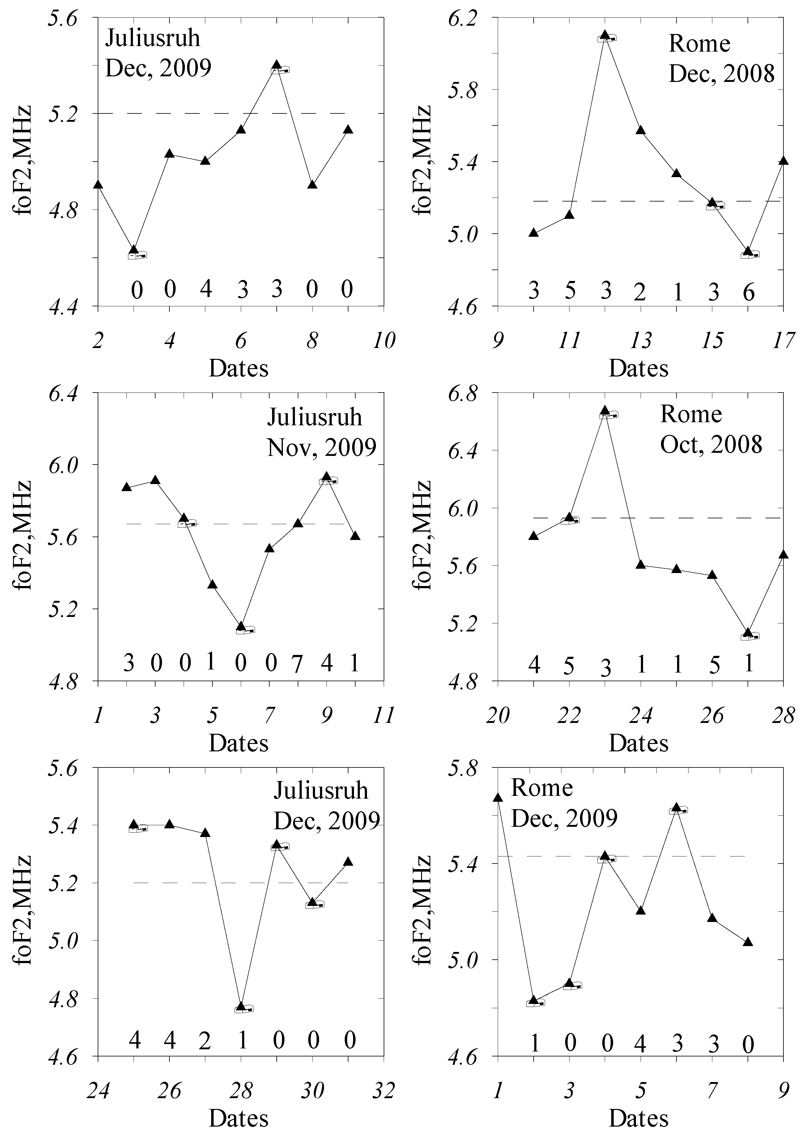
The (2008–2009) period with foF2 observations at the Rome and Juliusruh (located in one longitudinal sector) stations was checked to find events corresponding to the following requirements. Pronounced adjoining positive and negative foF2 deviations from the median level should take place within some days. Magnetic activity should be at a very low level for all days in question. The intensity of EUV radiations should also manifest small variations for the analyzed days. Selected cases of this type are given in Figure 1.
In general, ‘meteorological’ foF2 effects are of less magnitude compared to the Q-disturbance cases analyzed in [4]; foF2 deviations of ± 1 MHz are at their best. Therefore, we tried to find cases with maximal deviations within a month omitting lots of others with less magnitude. The observed foF2 variations (Figure 1) are presumably not related to geomagnetic activity, which was at a very low level (numbers at the bottom of panels); they also do not manifest QTD variations considering maximal and minimal foF2 values inside the analyzed periods. No system in the selected foF2 deviations has been found. The method from [24] was applied to the selected dates and the results are given in Table 1.
Figure 1 and Table 1 and Table 2 manifest that NmF2 deviations Δ = (δNmF2 − 1.0) may be both positive and negative. Observed EUV variations which mainly follow (F + F81)/2 [37] are small and unable to explain the observed NmF2 variations. The sign of Δ deviations is determined by the concentration of atomic oxygen. Positive Δ deviations correspond to larger [O]300 (bold font in Table 1 and Table 2), while negative Δ deviations correspond to smaller [O]300 (normal font). The correlation coefficient between NmF2 and [O]300 is 0.757 ± 0.314, which is significant at a 99.9% confidence level. Therefore, day-to-day variations of atomic oxygen provide the main contribution to NmF2 variations for the events given in Table 1 and Table 2. This is not a surprise bearing in mind that NmF2 ~[O]4/3 [38]. The contribution of other parameters is less significant. All days in question are characterized by negative (downward) vertical plasma drifts W corresponding to poleward thermospheric wind Vnx. Vertical drifts are more positive (a weaker poleward Vnx) for days with positive NmF2 deviations, and downward W is stronger for days with negative NmF2 deviations. The height of F2-layer maximum, hmF2, is known to be strongly controlled by vertical drift and neutral temperature, see, e.g., [39]. Days with positive Δ deviations manifest larger hmF2 and vice versa (Table 1 and Table 2). The magnitude of Tex variations is small and no system in its variations is seen. Therefore, under very low geomagnetic activity and practically invariable solar EUV radiation, day-to-day NmF2 variations are mainly due to day-to-day changes in atomic oxygen concentration at F2-region heights. The controlling role of atomic oxygen in the formation of large F2-layer daytime Q-disturbances was stressed earlier [2,3,4]. On the other hand, there is no confidence that the analyzed F2-layer perturbations have a meteorological origin.
2.2. SSW Event in January 2009
An excellent example of real meteorological impact on F2-region exhibit sudden stratospheric warming (SSW) events. SSW is a large-scale disturbance in the middle atmosphere, which is caused by the interaction between quasi-stationary planetary waves and the zonal mean flow [40]. This is a large-scale meteorological process in winter hemisphere which may last days or weeks [41]. The major SSW event in January 2009 is ideal to study the F2-layer reaction to lower atmospheric processes. During this event, solar and geomagnetic activity was at a very low level and the observed F2-layer long-term perturbations (not day-to-day variations) may be attributed to the impact from below. According to observations of the National Center for Environmental Predictions (NCEP), the peak warming at the 10 hPa level was reached on 23–24 January 2009 with stratospheric temperatures at 90° N having increased by more than 70 K. Previous considerations of this event [17,19,21] dealt with global TEC and COSMIC observations with the accent on low-latitude and equatorial ionosphere. We are considering European ground-based mid-latitude ionosonde and CHAMP neutral gas density observations to specify the F2-layer reaction to this SSW event.
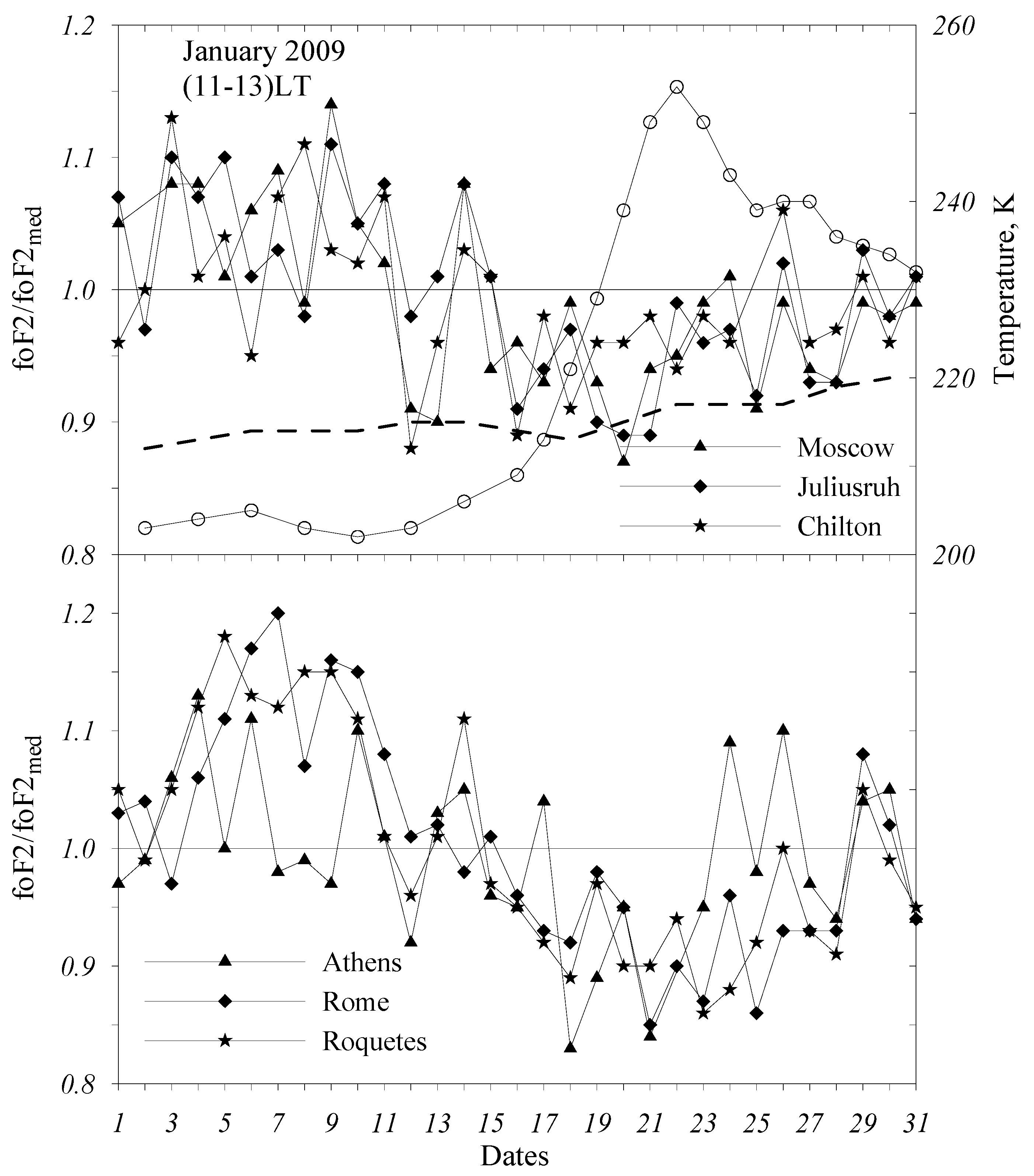
Previous analyses of SSWs have shown that this is a global phenomenon, and unlike earlier considered day-to-day foF2 variations which do not correlate at different stations, the ionospheric SSW effect should be seen simultaneously at all stations in question. To check this, we have divided our stations in two groups. A comparison of the higher latitude stations of Moscow, Juliusruh and Chilton to the lower latitude stations of Athens, Rome and Roquetes is given in Figure 2 for the foF2/foF2med ratio. Averaged over (11–13) LT, observed foF2 were used in this analysis. Stratospheric (10 hPa) temperature at high latitudes (60–90° N) in January 2009 along with the 30-year median is given in Figure 2. A pronounced depression in the foF2/foF2med ratio is seen in the vicinity of the SSW maximum development; however, the minimum is reached around 18–23 January, i.e., slightly before the SSW peak, contrary to the conclusion made in [18]. The minimum in NmF2 variations shortly before the peak of the SSW 2009 was also noted in [23].
Other authors [18] have revealed that the magnitude of ionospheric perturbations increases towards the equator. The foF2/foF2med variations for two groups of stations (Figure 2) do not differ significantly according to the Student criterion. However, the same groups of stations manifest different variations for the minor SSW 2008, confirming the conclusion [18] (Figure 5). This may tell us that the magnitude of foF2 depression (its latitudinal variation) depends on the intensity of SSW.
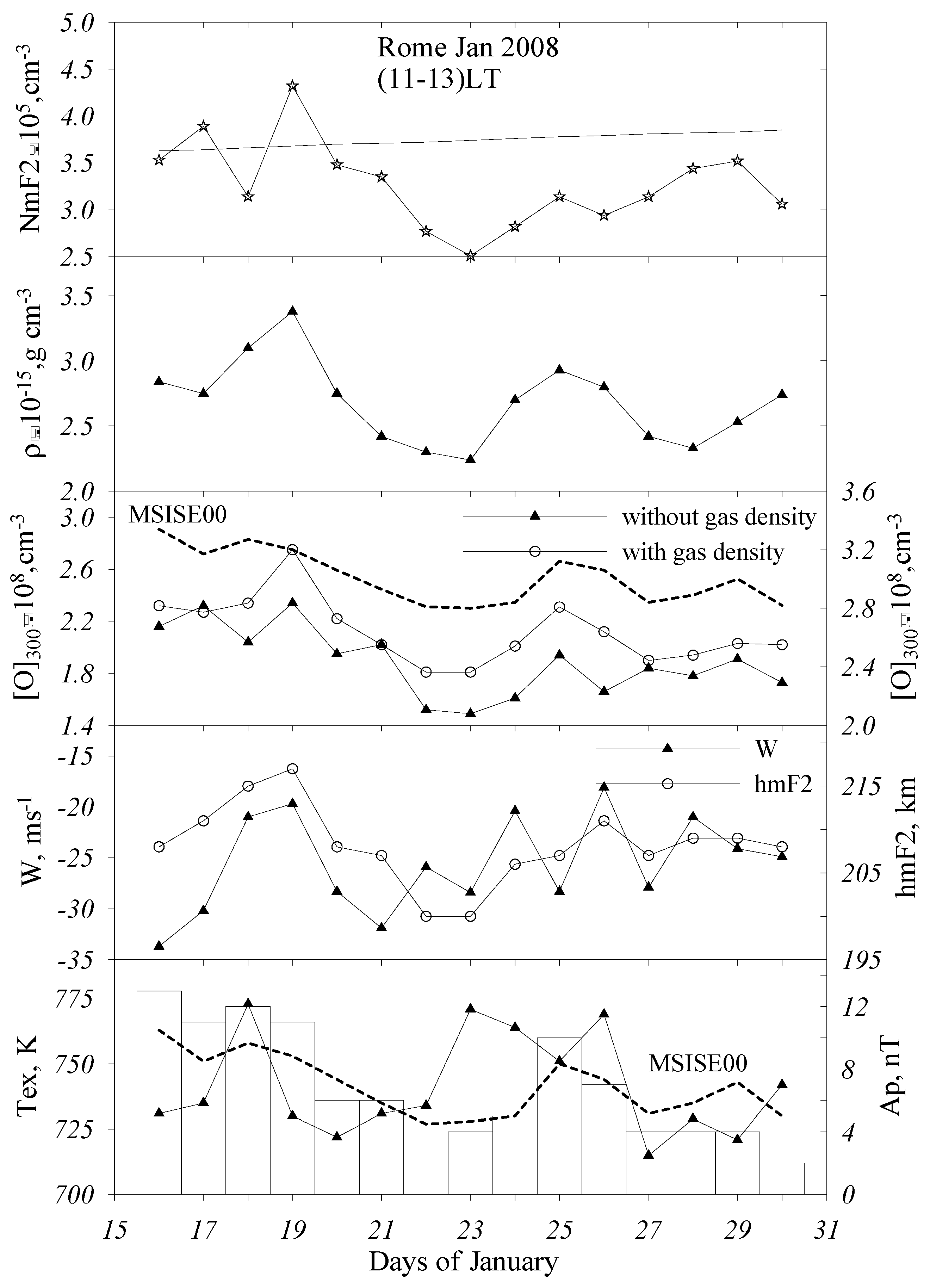
For the earlier-mentioned reason, Rome observations were selected for further analysis. Averaged over (11–13) LT, the daily foF2 variations are shown in Figure 3. Apart from small day-to-day foF2 changes, a long-term foF2 variation takes place in January 2009. Near-noontime foF2 observations manifest a well-pronounced depression in 20–28 January, which includes the period of maximal development of SSW in the stratosphere [17,42]. Initial (not reduced) CHAMP neutral gas density (ρ) observations in the European sector around Rome latitudes at (15–18) UT are given in a comparison to the MSISE00 [43] thermospheric model. Daily variations of the total EUV (100–1200) Å solar flux [25], along with Ap indices, are also given in Figure 3 to characterize the geophysical situation. The MSISE00 model, which is driven by solar and geomagnetic activity indices, gives quite different neutral gas density variations compared to CHAMP, without any depression on 22–24 January; moreover, the in general observed ρ values after 19 January are lower compared to the model ones (the upsurge on 26 January is due to the increase in geomagnetic activity). The magnitude of the observed EUV variations within the analyzed period is very small (~3%), being incomparable with the observed variations in foF2 and neutral gas density. Therefore, both foF2 and ρ indicate the SSW impact on the upper atmosphere and the ionospheric F2-region in accordance with the earlier obtained results [18,19,21,42,44,45], contrary to the conclusions in [22].
The method described in [24] was applied to the ionospheric near-noontime hour observations at Rome for January 2009. Two versions of our method were used to check the leading role of atomic oxygen in the analyzed variations of neutral gas density and ionospheric parameters. The basic version uses only observed electron concentration in the F1 and F2 layers. The extended version additionally uses observed neutral gas density (when available) as a fitted parameter. The retrieved aeronomic parameters, along with the observed NmF2 and geomagnetic indices, are given in Figure 4. MSISE00 model atomic oxygen and exospheric temperature variations are given for a comparison and further discussion.
Both versions are seen to give the depression in [O]300 variations with the minimum around the peak of SSW on 24 January (Figure 4). One may conclude that the retrieved [O]300 variations are not induced by the corresponding neutral gas density variations, but rather manifest the variations embedded in the observed electron concentration. The correlation coefficient between the observed NmF2 and the retrieved [O]300 (basic version of the method) is 0.840 ± 0.193 (R2 = 0.71), which is significant at the 99.9% confidence level. This means that ~70% of NmF2 variability is related to atomic oxygen variations. Retrieved atomic oxygen correlates with the observed neutral gas density with the correlation coefficient of 0.892 ± 0.134 (R2 ~0.8), being significant at the 99.9% confidence level. This means that 80% of neutral gas density variability is explained by atomic oxygen; the rest may be attributed to neutral temperature variations. Atomic oxygen is the main contributor to ρ at ~323 km—the height of the CHAMP measurements in Europe (January 2009).
MSISE00, which is driven by solar (F10.7) and geomagnetic (Ap) indices, predicts very small [O]300 variations during January 2009 with an average value of (2.67 ± 0.11) × 108 cm−3, and unlike the retrieved [O]300, indicates no pronounced depression in the vicinity of 23–24 January (Figure 4).
Both retrieved and MSISE00 Tex mainly follows Ap index variations, but the magnitude of retrieved Tex is larger (60–70 K), while MSISE00 retrieved a magnitude that is two times as small. A decrease in Tex of ~55 K is seen during 18–24 January (Figure 4), and this seemingly agrees with Millstone Hill ISR observations [16]. On the other hand, large thermospheric cooling by ~50 K during the SSW event in January 2009 [21] cannot be related to small variations of Ap indices (see MSISE00 Tex variations), as was supposed in [22]. Thus, the observed depression in neutral gas density during the SSW 2009 event (Figure 4) is mainly due to a decrease in the atomic oxygen concentration, while Tex variations play a secondary role.
Vertical plasma drift W, mainly related to meridional thermospheric wind, demonstrates some depression around the middle of January, i.e., the northward neutral wind increases along with the SSW development and reaches its maximum on 22 January, i.e., close to the SSW peak. The retrieved hmF2 at Rome clearly indicates a depression with the minimum around 23 January. The height of the F2-layer maximum mainly follows W variations during the analyzed period (Figure 4) as the dependence on atomic oxygen is weaker via logarithm and the absolute Tex changes are not large. The hmF2 dependence on aeronomic parameters is given by the following expression [39,46]:
where H = kT/mg—scale height, [O]1—concentration of neutral atomic oxygen at a fixed height h1 (say 300 km), β = γ1[N2] + γ2[O2]—linear loss coefficient, d = D × [O]1, D—ambipolar diffusion coefficient at h1 height and f(W)—an empirical expression obtained in [39] after the analysis of the Millstone Hill ISR observations. The hmF2 depression is around 10–15 km (Figure 4), which coincides with the results [18] obtained using COSMIC observations for the SSW 2009 event.
2.3. SSW Event in January 2008
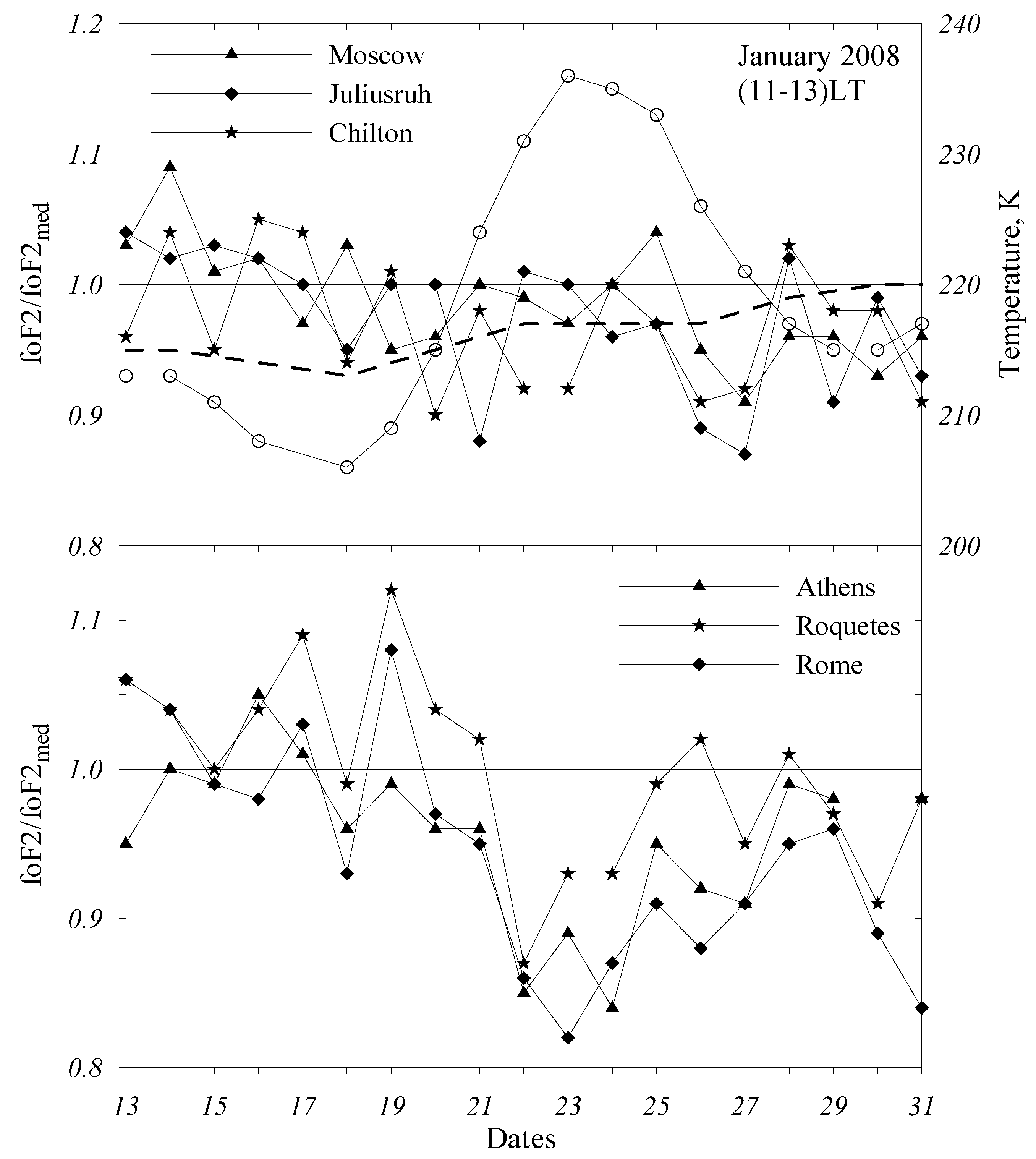
Unlike the January SSW 2009, which was the strongest and the longest-lasting major SSW recorded event, the January SSW 2008 was a minor one, presented by four separate warming periods [47], Figure 1. This difference was manifested in different ionospheric parameter variations during the two periods as this was shown by Pancheva and Mukhtarov [18]. Our analysis also confirms this difference. Higher latitude stations manifest a small (≤10%) foF2 depression around the SSW maximum development (Figure 5), while three lower latitude stations demonstrate a well-pronounced trough after 21 January. A comparison of the two groups of deviations after 21 January (the maximal warming took place around 23 January [47]) indicates a difference between two groups which is significant at the 98% confidence level according to the t-criterion.
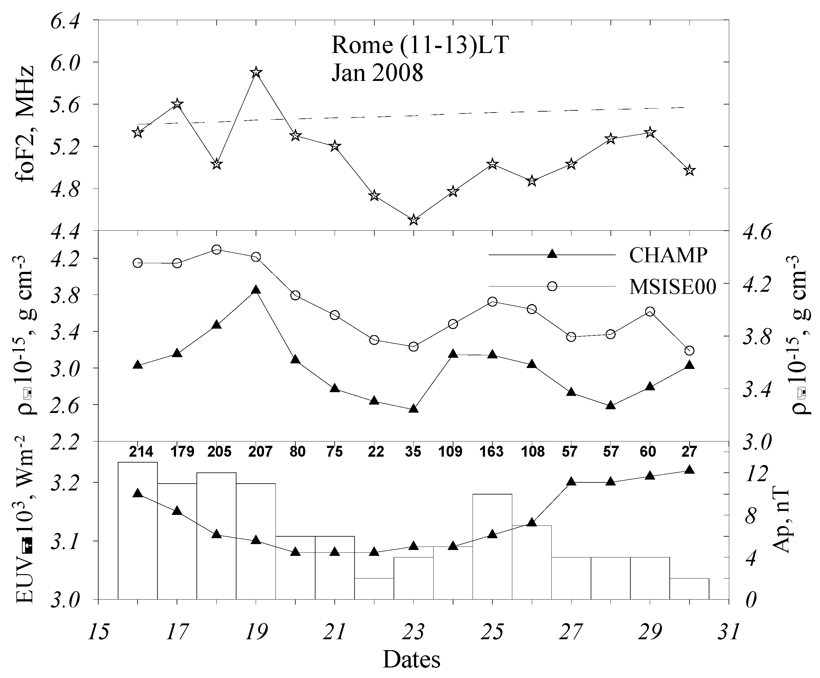
Rome observations are considered for the further analysis. Figure 6 indicates the foF2 depression depth of 25% (56% in NmF2) with respect to the median level is. This is incomparable to the magnitude of EUV variations—around 3%. MSISE00 model neutral gas density is seen to follow Ap index variations with a magnitude of ~19%, which is much less than the magnitude of the ρ variations (~52%) observed with CHAMP. Therefore, similar to the SSW 2009 event, both foF2 and neutral gas density manifest a pronounced depression in the vicinity of the SSW 2008 maximum development not related to EUV nor geomagnetic activity variations.
Ionospheric observations at Rome in January 2008 were developed with the method described in [24] to retrieve aeronomic parameters responsible for the observed NmF2 variations. The extracted parameters along with observed NmF2 neutral gas density, and geomagnetic indices are given in Figure 7. MSISE00 model atomic oxygen and exospheric temperature variations are given for the further discussion. Both versions of our method give [O]300 variations similar to the MSISE00 model ones with the minimum on 22–23 January following Ap index variations. However, a comparison of 16–17 January to 22–23 January gives a difference of ~49% for the retrieved [O] variations, and only a 16% difference for MSISE00 variations. We remind the reader that MSISE00 is driven by solar and geomagnetic activity indices. This means that the [O]300 depression around 22–23 January is only partly due to geomagnetic activity variations, while the main contribution is related to the SSW impact.
Similar to the SSW 2009 results, the correlation coefficient between the observed NmF2 and the retrieved [O]300 (basic version of the method) is 0.902 ± 0.159 (R2 = 0.81), which is significant at the 99.9% confidence level. This means that ~81% of NmF2 variability is related to atomic oxygen variations. The correlation coefficient between [O]300 and observed neutral gas density is 0.940 ± 0.099 (R2 = 0.88), i.e., 88% of the neutral gas density variability is explained by atomic oxygen, the rest may be attributed to neutral temperature variations. The undertaken analysis for the SSW 2008 has confirmed the conclusion that atomic oxygen provides the main contribution both to observed NmF2 and neutral gas density variations during both SSW events.
The retrieved hmF2 manifests a depression around 22–23 January, i.e., close to the maximal development of SSW mainly following vertical plasma drift W variations (Figure 7). Similar result was obtained for the SSW 2009 (Figure 4). Therefore, one may speak about a tendency for the northward thermospheric wind to increase with the SSW development.
The MSISE00 exospheric temperature (Figure 7, bottom panel) does manifest a depression on 22–23 January, which is related to low geomagnetic activity at that time. The retrieved Tex does not follow Ap index variations without a pronounced depression in the vicinity of the SSW maximal development.
3. Interpretation
Both day-to-day and SSW NmF2 variations were shown to be mainly related to atomic oxygen; however, these [O] variations may be due to different mechanisms. Under the deep solar minimum conditions in question, the rate of the O2 dissociation by the Schumann-Runge continuum may be considered as practically invariable (see small EUV variations in Table 1 and Table 2 and Figure 3). Moreover, the characteristic (e-fold) time of the O2 dissociation process is 1/JO2 ~3 days above 120 km height [36], while we use day-to-day variations; this implies a very fast redistribution of atomic oxygen. Therefore, there are some ways to change the atomic oxygen abundance in the thermosphere—via upwelling (downwelling), via eddy diffusion variations at the turbopause level and due to the enhancement of the migrating semidiurnal solar tide (SW2) during SSWs [23].
Let us consider the first possibility. Very quiet periods were selected to analyze the day-to-day variations of foF2 (Figure 1, Table 1 and Table 2) to exclude geomagnetic activity effects as much as possible. However, splashes of auroral activity took place even during such quiet periods and their effects are seen in foF2 variations. The analysis of positive and negative (with respect to monthly median) foF2 deviations (Figure 1) has shown that they are related to such splashes of auroral activity manifested by daily AE indices given in Table 1 and Table 2. Daily AE around 30 nT may be considered as a threshold. Negative foF2 deviations correspond to daily AE < 30 nT while positive foF2 deviations correspond to AE above this threshold. The only exclusion manifests 16 December 2008 at Rome when a small negative foF2 deviation took place under daily AE = 64 nT. However, at Juliusruh, this day is marked by a positive foF2 deviation in accordance with the formulated rule.
Such an foF2 reaction to auroral activity is in the framework of the mechanism considered in our previous analysis [4] for large Q-disturbances. This mechanism considers global thermospheric circulation as the main driver changing the atomic oxygen abundance. Negative F2-layer Q-disturbances are associated with extremely low level of magnetic activity corresponding to the minimal intensity of auroral heating (see the AE indices in Table 1 and Table 2). This situation corresponds to an unconstrained solar-driven thermospheric circulation (a strong poleward neutral Vnx wind) and to relatively low atomic oxygen concentrations at middle latitudes as this follows from the model simulations [48], Figure 3—low [O] may be related to a moderate upwelling of neutral gas in a wide range of latitudes. The retrieved downward W values for negative Q-disturbance days are larger compared to reference days. A decrease of atomic oxygen is seen both at 300 km (average [O]Qday/[O]ref = 0.92 ± 0.07) and in the column abundance (average [O]Qday/[O]ref = 0.91 ± 0.06).
A similar explanation may be given to positive Q-disturbance cases. Smaller vertical plasma drifts W on Q-disturbed days (Table 1 and Table 2) tell us that the northward circulation was damped. This should decrease upwelling, increasing in this way the atomic oxygen abundance in the thermosphere [48,49]. Indeed, the retrieved average [O]Qday/[O]ref ratio at 300 km is 1.14 ± 0.09 and the average [O]Qday/[O]ref ratio for column density is 1.10 ± 0.07.
Along with this, there is a mechanism based on model simulations [23,50]. According to this mechanism, an enhancement of the migrating semidiurnal solar tide (SW2) is the source of the variability in thermospheric composition. In particular, the enhancement of the SW2 during SSWs alters the lower thermosphere zonal mean circulation, leading to a reduction in atomic oxygen in the lower thermosphere. The efficiency of this mechanism should be yet demonstrated and confirmed at a quantitative level, for instance, how does it describe quiet time F2-layer disturbances? Furthermore, available NmF2 and satellite (CHAMP, GRACE) neutral gas density observations during SSW events could be successfully used to check the efficiency of this mechanism not qualitatively but quantitatively.
During the SSW 2009 and 2008 events, the day-to-day foF2 variations overlapped with the long-term foF2 variation with a well-pronounced depression in the vicinity of the SSW maximum development on 24 January (Figure 2 and Figure 5). Unlike the day-to-day foF2 variations, which as a rule do not correlate at different stations separated in longitude and latitude, the smoothed long-term foF2 variation is in-phase at all stations in question (Figure 2), confirming the global-scale SSW occurrence. It seems that the magnitude of the F2-layer reaction depends on the intensity (major or minor) SSW event (cf. Figure 2 and Figure 5).
The retrieved decrease of atomic oxygen abundance may be related to an increase of eddy diffusion during the SSW event [42,51]. The idea to use eddy diffusion to change the thermospheric neutral composition is not new [52,53,54]. Theoretically, it was shown that the maximal value of the time average eddy diffusion coefficient in the thermosphere cannot exceed 3 × 106 cm2/s [55] and this was confirmed experimentally—the annual mean eddy diffusion coefficient is ~4 × 106 cm2/s at 85–100 km [56]; the same estimate was obtained earlier in [52].
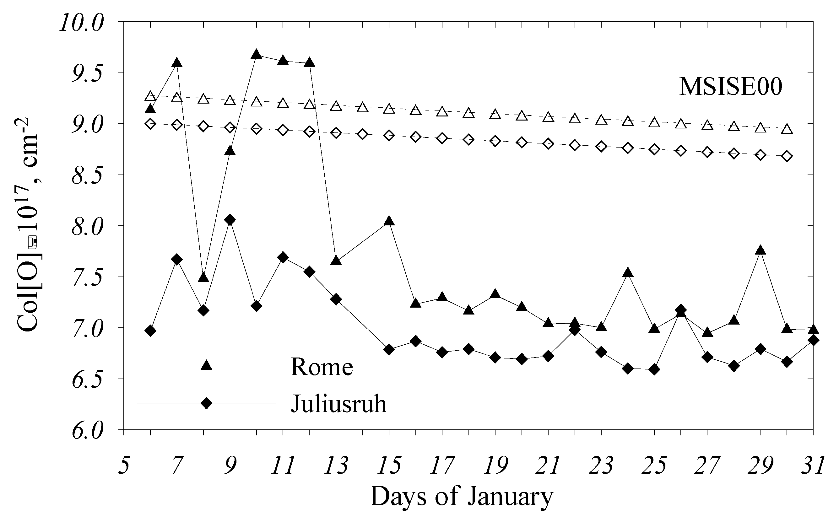
The calculated column content of atomic oxygen, [O]col, at Rome exhibits interesting variations (Figure 8). Until 16 January, [O]col manifested large day-to-day variations but later, [O]col reached a stable level of (7.16 ± 0.22) × 1017 cm−2 which was kept until the end of the period in question. Juliusruh manifested a similar type of [O]col variations. Model MSISE00, driven by solar and geomagnetic activity indices, exhibited quite different [O]col variations for the same period (Figure 8). Such [O]col variations may be interpreted in terms of the eddy diffusion mechanism. Theoretically, it was shown that the maximum value of the eddy diffusion coefficient was limited from above [55]; therefore, the plateau in [O]col variations after January 15 (Figure 8) may be related to the maximal Kedd reached in the course of the SSW 2009 event.
The eddy diffusion mechanism of decreasing the atomic oxygen abundance during the SSW 2009 is confirmed by observations in the ionospheric D-region. The intensification of eddy diffusion reduces [O] in the thermosphere; on the other hand, this increases the transfer of nitric oxide NO from the lower thermosphere to D-region heights [57,58]. Nitric oxide is efficiently ionized by a strong HLy emission increasing electron concentration in the D-region [59]. The effects of the major sudden stratospheric warming event of 2009 on the subionospheric very low frequency/low frequency (VLF/LF) radio signals propagating in the Earth-ionosphere waveguide over the North Atlantic and North Pacific regions in the Northern Hemisphere were presented by [60]. An increase of the signal amplitude at daytime was observed during the SSW event compared to normal days. Model simulations have shown that an increase of electron density and collision frequency from the standard IRI-model produce higher daytime VLF amplitude. The authors related this electron density increase in the lower ionosphere with downward plasma motion during the SSW period. Of course, this is impossible because plasma at D-region heights is strictly in photo-chemical equilibrium and cannot be transferred.
The eddy diffusion mechanism qualitatively also explains the thermosphere cooling around the peak of SSW (Figure 4). According to [61], vertically propagating internal gravity waves induce a downward transfer of heat from regions of wave dissipation, and this may result in a net cooling of the upper atmosphere. The mechanism of thermospheric cooling via eddy diffusion was also used in [62] to explain an inversion of neutral temperature in the lower thermosphere.
4. Discussion
The analysis of day-to-day foF2 variations during the deep solar minimum in 2008–2009 has confirmed our previous results [4] that both positive and negative foF2 deviations are due to atomic oxygen variations presumably related to day-to-day changes in the thermospheric circulation. The selection of deep solar minimum for our analysis has excluded the effects related to solar EUV variations. Indeed, the observed total ionizing solar flux [25] was practically constant manifesting very small day-to-day variations. Despite very low levels of magnetic activity, individual splashes seen in AE indices took place during the period in question, and daily AE > 30 nT (as a threshold) was sufficient to alter the global solar driven circulation pattern resulting in its turn in changes of the atomic oxygen abundance. Therefore, the controlling role of auroral (geomagnetic) activity in foF2 day-to-day variations is seen even under deep solar minimum. This is an interesting result telling us that the term ‘magnetically quiet conditions’ has a relative sense depending on the level of solar activity in question. The same daily Ap = 11 nT on 26 January 2009 will correspond quiet conditions under solar maximum, but has resulted in large deviations in thermospheric parameters during deep solar minimum (Figure 4). Figure 1 shows that pronounced foF2 variations took place under even lower level (Ap = 3–5 nT) of geomagnetic activity. This peculiarity was mentioned earlier in [63], where it was shown that at fixed heights, magnetic activity would have a larger relative effect on the neutral density under solar minimum due to smaller-scale heights. Nevertheless, one may think that pure meteorological effects (i.e., not related to solar and geomagnetic activity) in day-to-day foF2 variations related to planetary and gravity waves do exist, but a special selection of days with zero 3h-ap indices are required for such analysis and this is a task for future.
A major SSW in January 2009 should be considered as a lucky case to study pure meteorological impact on the thermosphere and ionosphere, as solar and geomagnetic activity was at the lowest level and observed long-term (for 2–3 weeks) perturbations of the upper atmosphere parameters should be attributed to the impact from below. Well-pronounced statistically significant effects have been observed in the ionosphere [17,18,19,20,23,64].
TEC, often used in SSW analyses, is an integral ionospheric characteristic which includes the plasmaspheric part not related by any means to the underlying F2-region; therefore, any physical interpretation of TEC variations is complicated and ambiguous. From this point of view, an analysis of Ne(h) profiles looks more preferable. However, different methods of analysis applied to the same COSMIC observations during the SSW 2009 event gave different morphological results. For instance, the authors [19] have revealed increases and decreases in NmF2 in different latitude/longitude and LT sectors. In particular, a (10–20)% NmF2 increase during daytime hours was found in the European sector analyzed in our paper. The authors in [20], analyzing COSMIC observations for the SSW 2009 event, have confirmed the global response of the ionosphere to this SSW event. They have revealed that the peak density (NmF2), peak height (hmF2) and ionospheric total electron content (ITEC) increase by 19%, 12 km and 17% in the morning (08–13) LT hours and decrease by 23%, 19 km and 25% in the afternoon. The COSMIC foF2 and hmF2 observations considered in [18] for the period of SSW in January 2009 revealed a global mean electron density response: foF2 manifested a decrease of 0.7–0.8 MHz, while the reduction in hmF2 was on average of 10–12 km.
Obviously, the results are strongly dependent on the selected background the deviations are counted from. It is not that easy to select a correct background level using RO satellite observations bearing in mind that deviations in foF2 and hmF2 may not be large. The analysis is simpler using local (not global) ground-based ionospheric observations. Taking foF2 observations over some solar cycles for (30–70) years, it is possible (see Introduction) to derive at a particular ionospheric station a climatologic empirical foF2 model which can be used as a background for a given month and level of solar activity. The results obtained on this way may be more confident.
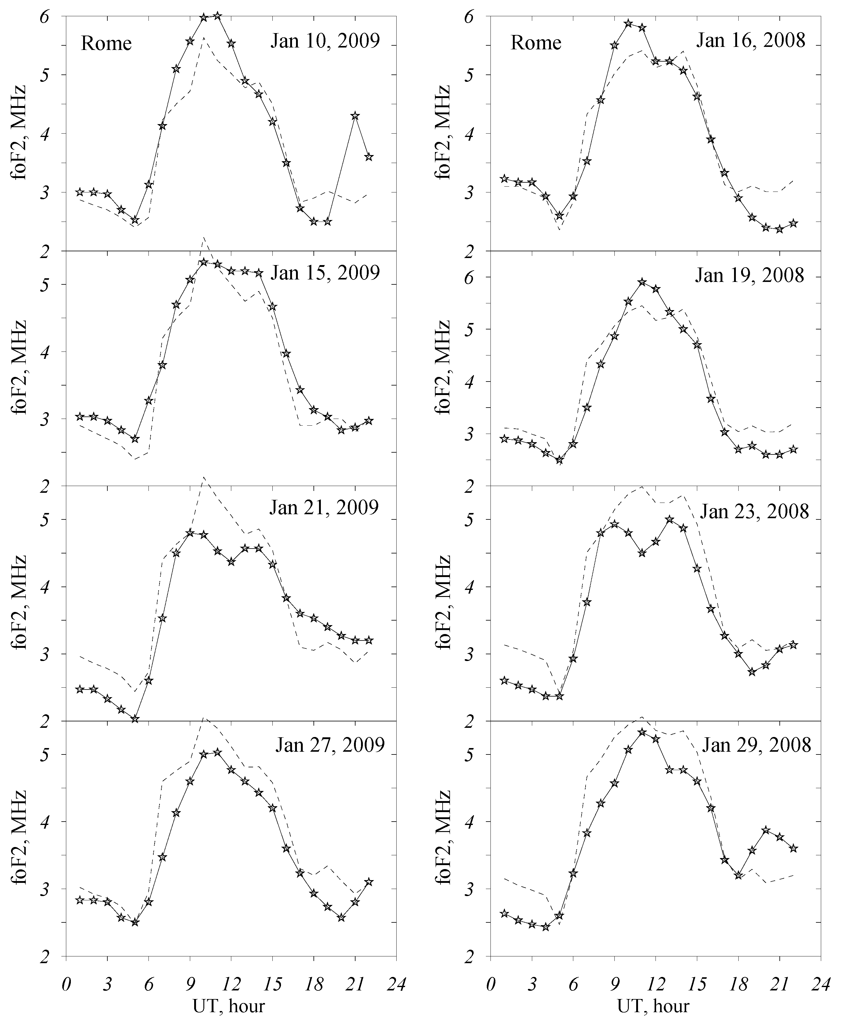
Figure 9 illustrates diurnal foF2 variations at Rome for days preceding and during the SSW 2008 and 2009 events (see also Figure 3 and Figure 6). Days preceding SSWs are marked by foF2, which are larger than or close to the monthly median values during daytime hours. However, days in the vicinity of the SSW maximum development (21 January 2009 and 23 January 2008) manifest a well-pronounced foF2 depression with the minimum around noontime. Both days demonstrate similar variations during early morning and daytime hours with foF2 lower median values contrary to the pattern revealed by [19,20]. Days 27 January 2009 and 29 January 2008 also manifest decreased foF2 during all daytime hours. Our analysis has shown that foF2 decrease on SSW days is due to a decrease in the atomic oxygen abundance—the main after EUV contributor to NmF2 in the upper atmosphere. This decrease in [O] is confirmed by a decrease in observed neutral gas density (Figure 4 and Figure 7). Under low [O] and strong downward plasma drifts (Figure 4 and Figure 7), it is impossible to have increased foF2 at middle latitudes during daytime, as mentioned by [19,20].
The major SSW 2009 event was also analyzed in [21] using CHAMP observations. Firstly, it should be stressed that, as revealed in [21], the decrease in neutral gas density and electron concentration at 325 km height is a real manifestation of SSW impact on the upper atmosphere, contrary to the opinion described in [22]. The effects of geomagnetic activity were too small in January 2009 to explain the observed variations in thermospheric parameters. Figure 3, Figure 4 and Figure 8 clearly show that MSISE00, which is driven by solar and geomagnetic activity indices, is unable to describe the variations of thermospheric parameters during the SSW 2009 event. The other issue is the interpretation of the observed effects. The authors in [21] have related the Ne decrease to thermospheric cooling and a decrease of plasma scale height. On the one hand, plasma scale height depends on plasma temperatures (Te and Ti) rather than on neutral temperature, Tn. Ion temperature, Ti, is close to Tn only below 200–250 km, while electron temperature Te is always larger than Tn at F-region heights (see for reference Millstone Hill ISR observations). On the other hand, NmF2, which is mapped to the topside mainly follows the constant pressure level [65] during daytime, manifesting a weak dependence on neutral temperature. Therefore, the observed with CHAMP Ne decrease in the F2-layer topside just reflects the NmF2 decrease at middle and lower latitudes. In the vicinity of the geomagnetic equator, this NmF2 decrease is due to counter electrojet [66,67] with downward ExB plasma drift during daytime hours; an additional NmF2 decrease is related to a reduced atomic oxygen concentration manifested in low neutral gas density, which is also observed with CHAMP for the SSW 2009 event.
The undertaken analysis of the NmF2 depression at middle latitudes during the SSW in 2009 and 2008 has shown that this depression is due to a reduction of the atomic oxygen concentration in the upper atmosphere. We are speaking not about a decrease of [O] at F2-region heights, which may be partly related to a decrease in neutral temperature, which also does take place during SSW 2009 (Figure 4), but about a decrease of the column abundance of atomic oxygen (Figure 8), which is independent from the temperature profile. This decrease of atomic oxygen is also responsible for the decrease of neutral gas density observed with CHAMP. Therefore, a mechanism of the atomic oxygen reduction during SSW events is a crucial issue.
Model simulations with TIE-GCM for the periods of SSWs have shown that the NmF2 decrease coincides with a depletion of thermospheric [O]/[N2], indicating that the NmF2 depletion is related to changes in thermospheric composition during SSWs [23]. The enhancement of the SW2 during SSWs alters the lower thermosphere zonal mean circulation, leading to a reduction in atomic oxygen in the lower thermosphere. This is an interesting and promising result. Moreover, the authors hypothesize that significant tidal variability during other time periods will have a similar impact on the ionosphere-thermosphere mean state. This means that the suggested mechanism could be used to explain day-to-day NmF2 variations. In any case, the mechanism requires a serious testing with a quantitative comparison to real NmF2 and satellite neutral gas density observations during SSWs periods. A comparison given in [23] indicates a difference in NmF2 by a factor of 2 between the model and observations and this is too much to accept the proposed mechanism as an explanation for the decrease in the atomic oxygen abundance. Moreover, the proposed mechanism should explain an increase of electron density at D-region heights during SSWs according to [60] observations.
A plausible explanation has been considered in [42]. The intensity of gravity waves increases during SSWs, e.g., Refs. [68,69]. The dissipation of upward propagating gravity waves in the mesosphere and lower thermosphere generates turbulence (eddy diffusion), which induces both a downward transport of heat and atomic oxygen. Although these effects of eddy diffusion are well-known, the application of this mechanism to explain the observed neutral gas density and NmF2 variations during SSW events should be considered as a proper step. Our analysis seems to confirm this approach. Figure 8 shows that the atomic oxygen column content decreases in the beginning of the SSW event, then reaches the plateau after 15 January and keeps this level until the end of the period in question. This plateau may tell us that the intensity of eddy diffusion has reached its maximum in accordance with the theoretical consideration [55] and any further decrease of atomic oxygen does not take place.
Usually observed decrease of thermospheric neutral gas density during SSWs is prescribed to corresponding decrease in neutral temperature [21,42], the thermospheric MSISE00 model [43] is used for such reduction. Neutral gas density at a given height depends both on neutral composition and temperature. Our analysis has shown that ~80% (SSW 2009) and ~88% (SSW 2009) of neutral gas density variability at the Rome location is explained by atomic oxygen variations, which is the main contributor to ρ at the height of CHAMP measurements in Europe (January 2008–2009); the rest may be attributed to neutral temperature variations. Therefore, a 50-K drop of neutral temperature used in [21] to explain the observed 30–45% decrease in neutral gas density should be considered as an overestimation.
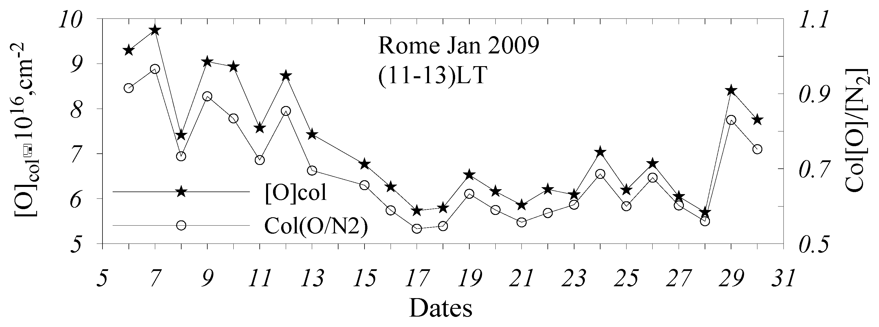
On the other hand, up to now, we have not had any direct confirmations of the reduction of atomic oxygen abundance during SSWs. Recent Global-Scale Observations of the Limb and Disk (GOLD) have revealed a 10% depletion in the O/N2 column density during the SSW event in early January 2019 [45]. The authors stress that the observed O/N2 column–density ratio depletion is not caused by geomagnetic activity variations. Although the authors in [45] described the O/N2 column density depletion, in fact, we are dealing with a pure reduction of the atomic oxygen abundance. It is well-known that N2 distribution in the thermosphere is close to a barometric distribution. On the one hand, N2 is a chemically inactive gas; on the other hand, its distribution is not practically affected by eddy diffusion, since the molecular weight of N2 is about the same as the average molecular weight of the mixed atmosphere, see, e.g., [53]. According to the method described in [70], the O/N2 column–density ratio is in reference to an N2 column density 1017 cm−2. In the case of the SSW event in 2009, this level does not exhibit strong variations at Rome, located at a (133 ± 1) km altitude.
In this case, the column [O]/[N2] ratio just follows the column [O] variations (Figure 10). The retrieved column [O]/[N2] ratio manifests a ~50% depletion, i.e., larger than what was observed for the SSW 2019 event [37]. The observations in [45] may be considered as an experimental confirmation to our results on the atomic oxygen depletion during SSWs. However, these observations only tell us that the atomic oxygen abundance does decrease in the course of SSWs, but they do not tell us anything about the mechanism of this [O] depletion, which is discussed in [45].
5. Conclusions
European near-noontime ionosonde observations were analyzed during the period deep solar minimum in 2008–2009 to reveal foF2 deviations not related to solar and geomagnetic activity variations. Day-to-day and long-term foF2 variations during the SSW in 2009 and 2008 were analyzed to understand the formation mechanisms of the observed foF2 deviations. The original method [24] was applied to ionospheric observations to retrieve aeronomic parameters responsible for the observed foF2 variations. The obtained results may be summarized as follows.
- Day-to-day quiet time foF2 perturbations are mainly due to atomic oxygen variations. Days with negative foF2 deviations correspond to a decreased atomic oxygen abundance both at 300 km (average [O]/[O]ref = 0.92 ± 0.07) and in the column—average [O]/[O]ref = 0.91 ± 0.06. Positive foF2 deviations correspond to average [O]/[O]ref = 1.14 ± 0.09 at 300 km and [O]/[O]ref = 1.10 ± 0.07 in the column density.
- Some contribution to day-to-day foF2 variations provides vertical plasma drift W, which is more positive (a weaker poleward thermospheric neutral wind) for days with positive foF2 deviations, while downward W is stronger for days with negative foF2 deviations. Therefore, days with positive foF2 deviations manifest larger hmF2 and vice versa due to a strong hmF2 dependence on W.
- Despite very low geomagnetic activity, splashes of auroral activity seen in AE index variations took place during the analyzed periods. Negative foF2 deviations correspond to daily AE < 30 nT, while positive foF2 deviations correspond to daily AE above this threshold. Physically low geomagnetic activity (AE < 30 nT) corresponds to low auroral heating. The latter corresponds to an unconstrained solar-driven thermospheric circulation with a strong poleward thermospheric neutral wind Vnx and to a relatively low atomic oxygen concentration at middle latitudes due to upwelling [48]. Both factors (low [O] and strong downward plasma drift W = VnxsinIcosI) decrease NmF2, resulting in negative F2-layer disturbances. On the contrary, enhanced geomagnetic activity (AE >30 nT) with increased auroral heating damps the northward circulation during daytime hours, increasing the atomic oxygen abundance at middle latitudes due to less intensive upwelling. Both factors increase NmF2, resulting in positive F2-layer disturbances. Therefore, the controlling role of geomagnetic activity in foF2 day-to-day variations is seen even under deep solar minimum.
- In accordance with earlier published results, mid-latitude inospheric stations manifest a pronounced foF2 depression during the SSW 2009 and 2008 events with the magnitude of foF2/foF2med ratio increasing towards the equator. The retrieved hmF2 also demonstrate a decrease of 10–15 km with the minimum reached close to the maximal phase of the SSW development.
- Both the neutral gas density and retrieved atomic oxygen observed with CHAMP manifest a pronounced depression during the SSW events in January 2009 and 2008. The correlation coefficient between the retrieved [O]300 and observed neutral density is 0.892 ± 0.134 (R2 ~0.80) for SSW 2009 and 0.940 ± 0.099 (R2 ~0.88) for SSW 2008. This means that (80–88)% of neutral gas density variability can be explained by atomic oxygen variations; the rest may be attributed to neutral temperature variations. The correlation coefficient between observed NmF2 and the retrieved [O]300 is 0.840 ± 0.192 (R2 = 0.71) for SSW 2009 and 0.902 ± 0.159 (R2 ~0.81), i.e., ~(70–80)% of NmF2 variability is related to atomic oxygen variations. MSISE00, which is driven by solar (F10.7) and geomagnetic (Ap) indices, predicts very small [O]300 variations without any depression in the vicinity of the maximal phase of the SSW development.
- The undertaken analysis has shown the leading role of atomic oxygen in neutral gas density and NmF2 variations in the course of SSW. An experimental support to this result provides recent GOLD observations [45]. For the first time, a 10% depletion was directly observed the in O/N2 column density during the SSW event in early January 2019, and this O/N2 decrease was not caused by geomagnetic activity.
- An intensification of eddy diffusion during SSW events is suggested as a mechanism to explain a decrease of the atomic oxygen abundance and a related decrease in neutral gas density and in NmF2. An indirect confirmation to the eddy diffusion mechanism may serve an increase of the electron concentration in the ionospheric D-region during the SSW 2009 [60]. The increase of Ne may be related to the NO transfer from the lower thermosphere to D-region heights.
Author Contributions
Conceptualization, A.V.M.; methodology, A.V.M.; software, A.V.M. and L.P.; ionosonde and satellite data preparation, L.P. and A.A.N.; writing, A.V.M., L.P. and A.A.N. All authors have read and agreed to the published version of the manuscript.
Funding
This research was funded by INGV Project Pianeta Dinamico (CUP D53J19000170001) fund by MIUR (law 145/2018)—Task XX.
Institutional Review Board Statement
Not applicable.
Informed Consent Statement
Not applicable.
Data Availability Statement
In this study, we used the following observational data ionosonde data from Rome accessible from http://www.eswua.ingv.it/ and Juliusruh accessible from GIRO database http://giro.uml.edu/; satellite data from CHAMP accessible from ftp://[email protected]/champ/; EUV observations from http://lasp.colorado.edu/lisird/). Derived results are stored in an internal INGV archive data and can be requested by contacting the first author
Acknowledgments
The Rome ionospheric data are kindly provided by INGV (http://www.eswua.ingv.it/). The authors thank the GFZ German Research Center for CHAMP data (ftp://[email protected]/champ/) and Woods for EUV observations (http://lasp.colorado.edu/lisird/).
Conflicts of Interest
The authors declare no conflict of interest.
References
- Mikhailov, A.V. Morphology of quiet time F2-layer disturbances: High and lower latitudes. Int. J. Geomagn. Aeron. 2004, 5, 1006. [Google Scholar] [CrossRef]
- Mikhailov, A.V.; Depueva, A.H.; Depuev, V.H. Daytime F2-layer negative storm effect: What is the difference between storm-induced and Q-disturbance events? Ann. Geophys. 2007, 25, 1531–1541. [Google Scholar] [CrossRef] [Green Version]
- Mikhailov, A.V.; Depuev, V.K.; Depueva, A.K. Synchronous NmF2 and NmE daytime variations as a key to the mechanism of quiet-time F2-layer disturbances. Ann. Geophys. 2007, 25, 483–493. [Google Scholar] [CrossRef] [Green Version]
- Perrone, L.; Mikhailov, A.V.; Nusinov, A.A. Daytime mid-latitude F2-layer Q-disturbances: A formation mechanism. Sci. Rep. 2020, 10, 9997. Available online: https://www.nature.com/articles/s41598-020-66134-2 (accessed on 14 April 2021). [CrossRef] [PubMed]
- Forbes, J.; Zhang, X. Quasi 2-day oscillation of the ionosphere: A statistical study. J. Atmos. Solar-Terr. Phys. 1997, 59, 1025–1034. [Google Scholar] [CrossRef]
- Forbes, J.M.; Palo, S.E.; Zhang, X. Variability of the ionosphere. J. Atmos. Solar-Terr. Phys. 2000, 62, 685–693. [Google Scholar] [CrossRef]
- Rishbeth, H.; Mendillo, M. Patterns of F2-layer variability. J. Atmos. Solar-Terr. Phys. 2001, 63, 1661–1680. [Google Scholar] [CrossRef]
- Rishbeth, H. F-region links with the lower atmosphere? J. Atmos. Solar-Terr. Phys. 2006, 68, 469–478. [Google Scholar] [CrossRef]
- Fuller-Rowell, T.J.; Codrescu, M.; Wilkinson, P. Quantitative modelling of the ionospheric response to geomagnetic activity. Ann. Geophys. 2000, 18, 766–781. [Google Scholar] [CrossRef]
- Danilov, A.D. Meteorological control of the D-region. Ionos. Res. 1986, 39, 33–42. (In Russian) [Google Scholar]
- Kazimirovsky, E.; Herraiz, M.; De La Morena, B.A. Effects on the Ionosphere Due to Phenomena Occurring Below it. Surv. Geophys. 2003, 24, 139–184. [Google Scholar] [CrossRef]
- Lašťovička, J.; Križan, P.; Šauli, P.; Novotna, D. Persistence of the planetary wave type oscillations in foF2 over Europe. Ann. Geophys. 2003, 21, 1543–1552. [Google Scholar] [CrossRef] [Green Version]
- Altadill, D.; Apostolov, E.M.; Boška, J.; Laštovička, J.; Šauli, P. Planetary and gravity wave signatures in the F-region ionosphere with impact to radio propagation predictions and variability. Ann. Geophys. 2004, 47, 1109–1119. [Google Scholar]
- Nwankwo, V.U.; Chakrabarti, S.K. Effects of space weather on the ionosphere and LEO satellites’ orbital trajectory in equatorial, low and middle latitude. Adv. Space Res. 2018, 61, 1880–1889. [Google Scholar] [CrossRef]
- Altadill, D.; Sole, J.G.; Apostolov, E.M. First observation of quasi-2-day oscillations in ionospheric plasma frequency at fixed heights. Ann. Geophys. 1998, 16, 609–617. [Google Scholar] [CrossRef]
- Goncharenko, L.; Zhang, S.-R. Ionospheric signatures of sudden stratospheric warming: Ion temperature at middle latitude. Geophys. Res. Lett. 2008, 35. [Google Scholar] [CrossRef] [Green Version]
- Goncharenko, L.P.; Chau, J.L.; Liu, H.-L.; Coster, A.J. Unexpected connections between the stratosphere and ionosphere. Geophys. Res. Lett. 2010, 37, L10101. [Google Scholar] [CrossRef]
- Pancheva, D.; Mukhtarov, P. Stratospheric warmings: The atmosphere–ionosphere coupling paradigm. J. Atmos. Solar-Terr. Phys. 2011, 73, 1697–1702. [Google Scholar] [CrossRef]
- Oyama, K.; Jhou, J.T.; Lin, J.T.; Lin, C.C.H.; Liu, H.; Yumoto, K. Ionospheric response to 2009 sudden stratospheric warming in the Northern Hemisphere. J. Geophys. Res. Space Phys. 2014, 119, 10260–10275. [Google Scholar] [CrossRef] [Green Version]
- Yue, X.; Schreiner, W.S.; Lei, J.; Rocken, C.; Hunt, D.C.; Kuo, Y.-H.; Wan, W. Global ionospheric response observed by COSMIC satellites during the January 2009 stratospheric sudden warming event. J. Geophys. Res. Space Phys. 2010, 115, A00G09. [Google Scholar] [CrossRef] [Green Version]
- Liu, H.; Doornbos, E.; Yamamoto, M.; Ram, S.T. Strong thermospheric cooling during the 2009 major stratosphere warming. Geophys. Res. Lett. 2011, 38. [Google Scholar] [CrossRef] [Green Version]
- Fuller-Rowell, T.; Akmaev, R.; Wu, F.; Fedrizzi, M.; Viereck, R.A.; Wang, H. Did the January 2009 sudden stratospheric warming cool or warm the thermosphere? Geophys. Res. Lett. 2011, 38, L18104. [Google Scholar] [CrossRef]
- Pedatella, N.M.; Richmond, A.D.; Maute, A.; Liu, H.-L. Impact of semidiurnal tidal variability during SSWs on the mean state of the ionosphere and thermosphere. J. Geophys. Res. Space Phys. 2016, 121, 8077–8088. [Google Scholar] [CrossRef] [Green Version]
- Perrone, L.; Mikhailov, A.V. A New Method to Retrieve Thermospheric Parameters From Daytime Bottom-Side Ne(h) Observations. J. Geophys. Res. Space Phys. 2018, 123, 10200–10212. [Google Scholar] [CrossRef]
- Woods, T.N.; Eparvier, F.G.; Harder, J.; Snow, M. Decoupling Solar Variability and Instrument Trends Using the Multiple Same-Irradiance-Level (MuSIL) Analysis Technique. Sol. Phys. 2018, 293, 76. [Google Scholar] [CrossRef] [PubMed] [Green Version]
- Wrenn, G.; Rodger, A.; Rishbeth, H. Geomagnetic storms in the Antarctic F-region. I. Diurnal and seasonal patterns for main phase effects. J. Atmos. Terr. Phys. 1987, 49, 901–913. [Google Scholar] [CrossRef]
- Perrone, L.; Pietrella, M.; Zolesi, B. A prediction model of foF2 over periods of severe geomagnetic activity. Adv. Space Res. 2007, 39, 674–680. [Google Scholar] [CrossRef]
- Pietrella, M.; Perrone, L. A local ionospheric model for forecasting the critical frequency of the F2 layer during disturbed geomagnetic and ionospheric conditions. Ann. Geophys. 2008, 26, 323–334. [Google Scholar] [CrossRef] [Green Version]
- Pietrella, M. A short-term ionospheric forecasting empirical regional model (IFERM) to predict the critical frequency of the F2 layer during moderate, disturbed, and very disturbed geomagnetic conditions over the European area. Ann. Geophys. 2012, 30, 343–355. [Google Scholar] [CrossRef] [Green Version]
- Shubin, V.N.; Annakuliev, S.K. Ionospheric storm negative phase model at middle latitudes. Geomag. Aeronom. 1995, 35, 363–369. [Google Scholar]
- Araujo-Pradere, E.A.; Fuller-Rowell, T.J.; Codrescu, M.V. STORM: An empirical storm-time ionospheric correction model 1. Model description. Radio Sci. 2002, 37, 1070. [Google Scholar] [CrossRef] [Green Version]
- Mikhailov, A.V.; Perrone, L. A method forfoF2short-term (1–24 h) forecast using both historical and real-timefoF2observations over European stations: EUROMAP model. Radio Sci. 2014, 49, 253–270. [Google Scholar] [CrossRef]
- Turner, J.F. The Development of the Ionospheric Index T, IPS Series R, Report, R11, Sydney. 1968. [Google Scholar]
- Caruana, J. The IPS monthly T index, Solar-Terrestrial Predictions. Proc. Workshop Leura Aust. Oct. 1990, 16–20, 257–263. [Google Scholar]
- Reinisch, B.W.; Galkin, I.A.; Khmyrov, G.; Kozlov, A.; Kitrosser, D.F. Automated collection and dissemination of ionospheric data from the digisonde network. Adv. Radio Sci. 2004, 2, 241–247. [Google Scholar] [CrossRef]
- Banks, P.M.; Kockarts, G. Aeronomy; Academic Press: New York, NY, USA; London, UK, 1973. [Google Scholar]
- Richards, P.G.; Fennelly, J.A.; Torr, D.G. EUVAC: A solar EUV flux model for aeronomic calculations. J. Geophys. Res. 1994, 99, 8981–8992. [Google Scholar] [CrossRef]
- Mikhailov, A.V.; Skoblin, M.G.; Förster, M. Day-time F2-layer positive storm effect at middle and lower latitudes. Ann. Geophys. 1995, 13, 532–540. [Google Scholar] [CrossRef]
- Perrone, L.; Mikhailov, A.V.; Scotto, C.; Sabbagh, D. Testing of the Method Retrieving a Consistent Set of Aeronomic Parameters With Millstone Hill ISR Noontime hₘF₂ Observations. IEEE Geosci. Remote. Sens. Lett. 2020, 1–3. [Google Scholar] [CrossRef]
- Andrews, D.; Holton, J.R.; Leovy, C.B. Stratospheric sudden warmings. In Middle Atmosphere Dynamics; Elsevier: New York, NY, USA, 1987; pp. 259–294. [Google Scholar]
- Matsuno, T. A Dynamical Model of the Stratospheric Sudden Warming. J. Atmos. Sci. 1971, 28, 1479–1494. [Google Scholar] [CrossRef]
- Yamazaki, Y.; Kosch, M.J.; Emmert, J.T. Evidence for stratospheric sudden warming effects on the upper thermosphere derived from satellite orbital decay data during 1967–2013. Geophys. Res. Lett. 2015, 42, 6180–6188. [Google Scholar] [CrossRef] [Green Version]
- Picone, J.M.; Hedin, A.E.; Drob, D.P.; Aikin, A.C. NRLMSISE-00 empirical model of the atmosphere: Statistical comparisons and scientific issues. J. Geophys. Res. Space Phys. 2002, 107, 1468. [Google Scholar] [CrossRef]
- Pedatella, N.M.; Maute, A. Impact of the semidiurnal lunar tide on the midlatitude thermospheric wind and ionosphere during sudden stratosphere warmings. J. Geophys. Res. Space Phys. 2015, 120, 10740–10753. [Google Scholar] [CrossRef]
- Oberheide, J.; Pedatella, N.M.; Gan, Q.; Kumari, K.; Burns, A.G.; Eastes, R.W. Thermospheric Composition O/N Response to an Altered Meridional Mean Circulation During Sudden Stratospheric Warmings Observed by GOLD. Geophys. Res. Lett. 2020, 47, e2019GL086313. [Google Scholar] [CrossRef]
- Ivanov-Kholodny, G.S.; Mikhailov, A.V. The Prediction of Ionospheric Conditions; D. Reidel Publishing Company Dordrecht: Dordrecht, The Netherlands, 1986. [Google Scholar]
- Chau, J.L.; Aponte, N.A.; Cabassa, E.; Sulzer, M.P.; Goncharenko, L.; Gonzalez, S.A. Quiet time ionospheric variability over Arecibo during sudden stratospheric warming events. J. Geophys. Res. Space Phys. 2010, 115, A00G06. [Google Scholar] [CrossRef]
- Rishbeth, H.; Müller-Wodarg, I.C.F. Vertical circulation and thermospheric composition: A modelling study. Ann. Geophysicae. 1999, 17, 794–805. [Google Scholar] [CrossRef]
- Rishbeth, H. How the thermospheric circulation affects the ionospheric F2-layer. J. Atmos. Solar-Terr. Phys. 1998, 60, 1385–1402. [Google Scholar] [CrossRef]
- Yamazaki, Y.; Richmond, A.D. A theory of ionospheric response to upward-propagating tides: Electrodynamic effects and tidal mixing effects. J. Geophys. Res. Space Phys. 2013, 118, 5891–5905. [Google Scholar] [CrossRef] [Green Version]
- Lindzen, R.S. Turbulence and stress owing to gravity wave and tidal breakdown. J. Geophys. Res. Space Phys. 1981, 86, 9707–9714. [Google Scholar] [CrossRef] [Green Version]
- Colegrove, F.D.; Hanson, W.B.; Johnson, F.S. Eddy diffusion and oxygen transport in the lower thermosphere. J. Geophys. Res. Space Phys. 1965, 70, 4931–4941. [Google Scholar] [CrossRef]
- Shimazaki, T. Effective eddy diffusion coefficient and atmospheric composition in the lower thermosphere. J. Atmos. Terr. Phys. 1971, 33, 1383–1401. [Google Scholar] [CrossRef]
- Schuchardt, K.G.H.; Blum, P.W. Correlation between the homopause height and density variations in the upper atmospheres. Space Res. 1977, 13, 335–340. [Google Scholar]
- Gordiets, B.F.; Kulikov, Y.N.; Markov, M.N.; Marov, M.Y. Numerical modelling of the thermospheric heat budget. J. Geophys. Res. Space Phys. 1982, 87, 4504. [Google Scholar] [CrossRef]
- Liu, A.Z. Estimate eddy diffusion coefficients from gravity wave vertical momentum and heat fluxes. Geophys. Res. Lett. 2009, 36, L08806. [Google Scholar] [CrossRef] [Green Version]
- Brasseur, G.; Nicolet, M. Chemospheric processes of nitric oxide in the mesosphere and stratosphere. Planet. Space Sci. 1973, 21, 939–961. [Google Scholar] [CrossRef]
- Richards, P.G. On the increases in nitric oxide density at midlatitudes during ionospheric storms. J. Geophys. Res. Space Phys. 2004, 109, A06304. [Google Scholar] [CrossRef]
- Whitten, R.C.; Poppoff, I.G. Fundaments of Aeronomy; J. Wiley & Sons, Inc.: New York, NY, USA; London, UK; Sydney, Australia; Toronto, ON, Canada, 1971. [Google Scholar]
- Pal, S.; Hobara, Y.; Chakrabarti, S.K.; Schnoor, P.W. Effects of the major sudden stratospheric warming event of 2009 on the subionospheric very low frequency/low frequency radio signals. J. Geophys. Res. Space Phys. 2017, 122, 7555–7566. [Google Scholar] [CrossRef]
- Walterscheid, R.L. Dynamical cooling induced by dissipating internal gravity waves. Geophys. Res. Lett. 1981, 8, 1235–1238. [Google Scholar] [CrossRef]
- Kolesnik, A.G.; Korolev, S.S.; Pasynkov, S.G. About temperature inversion of the thermosphere. Geomag. Aeron. 1982, 22, 435–439. (In Russian) [Google Scholar]
- Emmert, J.T.; Picone, J.M. Climatology of globally averaged thermospheric mass density. J. Geophys. Res. Space Phys. 2010, 115, A09326. [Google Scholar] [CrossRef] [Green Version]
- Gupta, S.; Upadhayaya, A.K. Morphology of ionospheric F 2 region variability associated with sudden stratospheric warmings. J. Geophys. Res. Space Phys. 2017, 122, 7798–7826. [Google Scholar] [CrossRef]
- Rishbeth, H.; Edwards, R. The isobaric F2-layer. J. Atmos. Terr. Phys. 1989, 51, 321–338. [Google Scholar] [CrossRef]
- Vineeth, C.; Pant, T.K.; Sridharan, R. Equatorial counter electrojets and polar stratospheric sudden warmings—A classical example of high latitude–low latitude coupling? Ann. Geophys. 2009, 27, 3147–3153. [Google Scholar] [CrossRef]
- Yamazaki, Y. Solar and lunar ionospheric electrodynamic effects during stratospheric sudden warmings. J. Atmos. Solar-Terr. Phys. 2014, 119, 138–146. [Google Scholar] [CrossRef]
- Hoffmann, P.; Singer, W.; Keuer, D.; Hocking, W.; Kunze, M.; Murayama, Y. Latitudinal and longitudinal variability of mesospheric winds and temperatures during stratospheric warming events. J. Atmos. Solar-Terr. Phys. 2007, 69, 2355–2366. [Google Scholar] [CrossRef]
- Yamashita, C.; Liu, H.-L.; Chu, X. Gravity wave variations during the 2009 stratospheric sudden warming as revealed by ECMWF-T799 and observations. Geophys. Res. Lett. 2010, 37, L22806. [Google Scholar] [CrossRef] [Green Version]
- Strickland, D.J.; Evans, J.S.; Paxton, L.J. Satellite remote sensing of thermospheric O/N2 and solar EUV 1. Theory. J. Geophys. Res. 1995, 100, 12217–12226. [Google Scholar] [CrossRef]
Figure 1.
Selected F2-layer Q-disturbances of the ‘meteorological’ origin. Monthly median foF2 are given with dashed lines. Circles—dates analyzed for the aeronomic parameters. Numbers at the bottom of panels—daily Ap indices.
Figure 1.
Selected F2-layer Q-disturbances of the ‘meteorological’ origin. Monthly median foF2 are given with dashed lines. Circles—dates analyzed for the aeronomic parameters. Numbers at the bottom of panels—daily Ap indices.

Figure 2.
The foF2/foF2med ratio for higher and lower latitude groups of stations during the SSW 2009 period. Solid lines indicate the monthly median level. Open circles—stratospheric (10 hPa) temperature at high latitudes (60–90°) N in January 2009. The dashed line represents the 30-year median value of the high latitude stratospheric temperature.

Figure 3.
Daily foF2 variations at Rome during the SSW event in January 2009. Dashes—model monthly median foF2 for 12 LT. The neutral gas density in the evening sector observed with CHAMP (left y-axis) is given in comparison to the MSISE00 model variations at the latitudes of Rome (right y-axis). Daily solar EUV (triangles) and Ap indices are given in the bottom panel. Numbers along x-axis (middle panel)—daily AE indices.

Figure 4.
The observed values averaged over (11–13) LT NmF2 at Rome (solid line in top panel—monthly median NmF2), measured with CHAMP neutral gas density reduced to the location of Rome and 12 LT, retrieved atomic oxygen at 300 km, vertical plasma drift, hmF2, and exospheric temperature are given in the plot. The daily AE values are given in the second panel and the daily Ap indices in the bottom panel. Dashed lines—MSISE00 model variations (right y-axis for [O]). Atomic oxygen was retrieved with (left y-axis) and without (right y-axis) fitting the observed neutral gas density.

Figure 5.
Same as Figure 2 but for the January SSW 2008 event.
Figure 5.
Same as Figure 2 but for the January SSW 2008 event.

Figure 6.
Same as Figure 3 but for the January 2008 SSW event.
Figure 6.
Same as Figure 3 but for the January 2008 SSW event.

Figure 7.
Same as Figure 4 but for the January 2008 SSW event.
Figure 7.
Same as Figure 4 but for the January 2008 SSW event.

Figure 8.
Retrieved column atomic oxygen abundance at Rome and Juliusruh in January 2009. Model MSISE00 variations are given with open symbols.
Figure 8.
Retrieved column atomic oxygen abundance at Rome and Juliusruh in January 2009. Model MSISE00 variations are given with open symbols.

Figure 9.
Observed averaged over (11–13) LT foF2 variations (asterisks) in a comparison with model monthly medians (dashes) at Rome for the events of SSW 2009 and 2008.
Figure 9.
Observed averaged over (11–13) LT foF2 variations (asterisks) in a comparison with model monthly medians (dashes) at Rome for the events of SSW 2009 and 2008.

Figure 10.
The retrieved column atomic oxygen density and column [O]/[N2] ratio, both in reference to an N2 column density of 1017 cm−2.
Figure 10.
The retrieved column atomic oxygen density and column [O]/[N2] ratio, both in reference to an N2 column density of 1017 cm−2.


Table 1.
Analyzed Q-disturbances of the ‘meteorological’ origin at Juliusruh. The table shows the observed half-sum of the daily and 81-day average F10.7, the daily Ap and AE indices, the observed values averaged over three (11–13) LT NmF2 (in 105 cm−3) along with δNmF2 = NmF2 Qday/NmF2 med (in brackets), the observed daily EUV, the calculated [O] column abundance, the retrieved exospheric Table 300 km along with δ[O] = [O]Qday/[O]med day (in brackets), the vertical plasma drift W and hmF2. Dates and data given in italic, which correspond to dates with NmF2 close to the monthly median NmF2.
| Date | (F + F81)/2 | Ap | NmF2 | EUVobs | [O]col, | Tex | [O]300 | W | hmF2 |
|---|---|---|---|---|---|---|---|---|---|
| (AE) | (δNmF2) | × 10−3 Wm−2 | × 1017 | K | × 108 | m s−1 | km | ||
| nT | cm−2 | cm−3 | |||||||
| 9 November 2009 | 72.8 | 4 | 4.37 | 3.09 | 9.46 | 737 | 3.02 | −25.2 | 214 |
| −68 | −1.08 | −1.03 | −1.19 | ||||||
| 6 November 2009 | 72 | 0 | 3.23 | 3.07 | 7.76 | 713 | 2.1 | −35.7 | 205 |
| −13 | −0.8 | −0.84 | −0.83 | ||||||
| 4 November 2009 | 72.1 | 4 | 4.03 | 3.11 | 9.18 | 719 | 2.54 | −29.5 | 208 |
| 7 December 2009 | 73.9 | 3 | 3.62 | 3.09 | 8.47 | 708 | 2.32 | −19.5 | 216 |
| −34 | −1.06 | −1.12 | −1.11 | ||||||
| 3 December 2009 | 73.9 | 0 | 2.66 | 3.07 | 7.56 | 694 | 1.85 | −37.7 | 203 |
| −12 | −0.78 | −1 | −0.89 | ||||||
| 18 December 2009 | 81 | 3 | 3.4 | 3.41 | 7.57 | 716 | 2.08 | −30.5 | 210 |
| 25 December 2009 | 77.5 | 4 | 3.62 | 3.38 | 8.63 | 704 | 2.32 | −25.9 | 212 |
| −33 | −1.11 | −1.1 | −1.3 | ||||||
| 28 December 2009 | 77.5 | 1 | 2.82 | 3.26 | 7.44 | 691 | 1.78 | −31.7 | 205 |
| −21 | −0.86 | −0.95 | −1 | ||||||
| 29 December 2009 | 76.7 | 0 | 3.53 | 3.23 | 7.92 | 687 | 1.83 | −20.4 | 212 |
| −15 | −1.08 | −1.01 | −1.03 | ||||||
| 30 December 2009 | 77.7 | 0 | 3.27 | 3.22 | 7.85 | 683 | 1.78 | −23.9 | 206 |
Table 2.
Same as Table 1 but for Rome.
Table 2.
Same as Table 1 but for Rome.
| Date | (F + F81)/2 | Ap | NmF2 | EUVobs | [O]col, | Tex | [O]300 | W | hmF2 |
|---|---|---|---|---|---|---|---|---|---|
| (AE) | (δNmF2) | × 10−3 | × 1017 | K | × 108 | m s−1 | km | ||
| nT | Wm−2 | cm−2 | cm−3 | ||||||
| 23 October 2008 | 67.7 | 3 | 5.51 | 3.08 | 8.63 | 735 | 2.56 | −9.3 | 226 |
| −43 | −1.26 | −1.17 | −1.06 | ||||||
| 27 October 2008 | 67.6 | 1 | 3.27 | 3.05 | 6.55 | 758 | 2.05 | −19.9 | 214 |
| −17 | −0.75 | −0.89 | −0.85 | ||||||
| 22 October 2008 | 67.9 | 5 | 4.37 | 3.13 | 7.39 | 756 | 2.42 | −9.7 | 230 |
| 12 December 2008 | 70.1 | 3 | 4.61 | 3.14 | 9.43 | 704 | 2.24 | −20.3 | 212 |
| −49 | −1.39 | −1.19 | −1.17 | ||||||
| 16 December 2008 | 69.3 | 6 | 2.98 | 3.09 | 7.12 | 717 | 1.85 | −35.4 | 203 |
| −64 | −0.9 | −0.9 | −0.96 | ||||||
| 15 December 2008 | 69 | 3 | 3.31 | 3.06 | 7.89 | 710 | 1.92 | −30.4 | 204 |
| 6 December 2009 | 74.2 | 3 | 3.94 | 3.11 | 8.65 | 725 | 2.28 | −25.7 | 210 |
| −32 | −1.08 | −1.05 | −1.13 | ||||||
| 2 December 2009 | 73.6 | 1 | 2.9 | 3.07 | 7 | 747 | 1.96 | −36.3 | 203 |
| −14 | −0.79 | −0.85 | −0.97 | ||||||
| 3 December 2009 | 73.9 | 0 | 2.98 | 3.07 | 7.77 | 724 | 1.95 | −37.2 | 203 |
| −12 | −0.81 | −0.94 | −0.96 | ||||||
| 4 December 2009 | 73.9 | 0 | 3.66 | 3.09 | 8.25 | 719 | 2.02 | −25.6 | 206 |
Publisher’s Note: MDPI stays neutral with regard to jurisdictional claims in published maps and institutional affiliations. |
© 2021 by the authors. Licensee MDPI, Basel, Switzerland. This article is an open access article distributed under the terms and conditions of the Creative Commons Attribution (CC BY) license (https://creativecommons.org/licenses/by/4.0/).
Share and Cite
MDPI and ACS Style
Mikhailov, A.V.; Perrone, L.; Nusinov, A.A. Mid-Latitude Daytime F2-Layer Disturbance Mechanism under Extremely Low Solar and Geomagnetic Activity in 2008–2009. Remote Sens. 2021, 13, 1514. https://doi.org/10.3390/rs13081514
AMA Style
Mikhailov AV, Perrone L, Nusinov AA. Mid-Latitude Daytime F2-Layer Disturbance Mechanism under Extremely Low Solar and Geomagnetic Activity in 2008–2009. Remote Sensing. 2021; 13(8):1514. https://doi.org/10.3390/rs13081514
Chicago/Turabian StyleMikhailov, Andrey V., Loredana Perrone, and Anatoly A. Nusinov. 2021. "Mid-Latitude Daytime F2-Layer Disturbance Mechanism under Extremely Low Solar and Geomagnetic Activity in 2008–2009" Remote Sensing 13, no. 8: 1514. https://doi.org/10.3390/rs13081514
Note that from the first issue of 2016, this journal uses article numbers instead of page numbers. See further details here.