
Regional Zenith Tropospheric Delay Modeling Based on Least Squares Support Vector Machine Using GNSS and ERA5 Data


1
School of Geological and Surveying Engineering, Chang’an University, Xi’an 710054, China
2
Institute of Space Science, Shandong University, Weihai 264209, China
*
Author to whom correspondence should be addressed.
Remote Sens. 2021, 13(5), 1004; https://doi.org/10.3390/rs13051004
Submission received: 6 January 2021
/
Revised: 24 February 2021
/
Accepted: 2 March 2021
/
Published: 6 March 2021
(This article belongs to the Special Issue Climate Modelling and Monitoring Using GNSS)
Abstract
:The meteorological reanalysis data has been widely applied to derive zenith tropospheric delay (ZTD) with a high spatial and temporal resolution. With the rapid development of artificial intelligence, machine learning also begins as a high-efficiency tool to be employed in modeling and predicting ZTD. In this paper, we develop three new regional ZTD models based on the least squares support vector machine (LSSVM), using both the International GNSS Service (IGS)-ZTD products and European Centre for Medium-Range Weather Forecasts Reanalysis 5 (ERA5) data over Europe throughout 2018. Among them, the ERA5 data is extended to ERA5S-ZTD and ERA5P-ZTD as the background data by the model method and integral method, respectively. Depending on different background data, three schemes are designed to construct ZTD models based on the LSSVM algorithm, including the without background data, with the ERA5S-ZTD, and with the ERA5P-ZTD. To investigate the advantage and feasibility of the proposed ZTD models, we evaluate the accuracy of two background data and three schemes by segmental comparison with the IGS-ZTD of 85 IGS stations in Europe. The results show that the overall average Root Mean Square Errors (RMSE) value of all sites is 30.1 mm for the ERA5S-ZTD, and 10.7 mm for the ERA5P-ZTD. The overall average RMSE is 25.8 mm, 22.9 mm, and 9 mm for the three schemes, respectively. Moreover, the overall improvement rate is 19.1% and 1.6% for the ZTD model with ERA5S-ZTD and ERA5P-ZTD, respectively. In order to explore the reason of the lower improvement for the ZTD model with ERA5P-ZTD, the loop verification is performed by estimating the ZTD values of each available IGS station. In actuality, the monthly improvement rate of estimated ZTD is positive for most stations, and the biggest improvement rate can even reach about 40%. The negative rate mainly comes from specific stations, these stations are located on the edge of the region, near the coast, as well as the lower similarity between the individual verified station and training stations.
1. Introduction
The troposphere constitutes most of the mass and water vapor of the entire atmosphere. The water vapor mainly concentrated in the troposphere below 10–12 km, which is an important meteorological factor causing climate change. With the rapid development of Global Navigation Satellite System (GNSS) technique, it has become an indispensable tool for monitoring water vapor variation [1,2]. When GNSS signals across the troposphere, these signals will slow down and bend because of the refraction of atmospheric molecules. The delay is usually described as the zenith tropospheric delay (ZTD) and the mapping function related to the elevation angle in the processing of GNSS data [3,4], and the water vapor variation can be retrieved and monitored by using high-precision ZTD values. Therefore, the ZTD model with high spatiotemporal resolution has great significance to the research of global climate change monitoring.
The classic ZTD models were based on the measured meteorological parameters, such as the Saastamoinen model [5] and the Hopfield model [6]. However, these models were mostly employed for post-event calculation because the measured meteorological data were not easy to obtain in some places or in real time. Later, some researchers studied the temporal and spatial characteristics of meteorological parameters to propose meteorological models, such as the University of New Brunswick (UNB) series models [7], European Geostationary Navigation Overlay System (EGNOS) model [8], and the Global Pressure/Temperature (GPT) series model [9,10,11]. In these models, latitude and time information were used to express relevant meteorological elements [12]. The user could obtain the corresponding meteorological parameters at the research area by interpolation and fitting, and then the ZTD value could be estimated by combining these meteorological parameters with the classic ZTD models. This way had the advantage to satisfy the needs of GNSS real-time positioning. However, owning to the complexity of the wet components in ZTD, it was difficult to establish the ZTD model solely based on fixed physical formulas to satisfy high precision applications.
Interestingly, machine learning algorithms were emerged to solve the modeling and prediction problems of nonlinear variation at the end of the 20th century. Among them, some models were constructed based on the neural network (NN) algorithms to depict the complex atmospheric parameters and worked well [13,14,15,16]. The NN algorithms were also applied into the modeling of tropospheric path delay. Katsougiannopoulos and Pikridas [17] employed the NN algorithms to predict ZTD for various time spans of one, three, and six hours, and the results of their predictions possessed the agreements of 2–3 cm with ZTD derived from the network of continuously operating GNSS in Europe. In addition, the adaptive neuron fuzzy inference system (ANFIS) algorithm was proposed to establish the ZTD model based on a single GNSS station, where the input and output parameters of the model was the surface meteorological data and the estimated ZTD values at the GNSS station, respectively [18,19]. Moreover, Xiao, et al. [20] optimized the hyper-parameters of the back propagation neural network (BPNN) algorithm to build the regional ZTD model in Japan, and this algorithm improved the fitting and prediction accuracy with Root Mean Square Errors (RMSE) of 7.8 mm and 8.5 mm, respectively. Furthermore, Zhang, et al. [21] derived an hourly high-accuracy ZTD model in west Antarctica by combining the BPNN algorithm, the long short-term memory (LSTM) network algorithm, as well as two blind source separation algorithms. Most existing ZTD models with the machine learning algorithms were based on the NN algorithms, but the NN algorithms may lead to a poor stability of performance and may be easy to fall into local minimum value.
The Least Squares Support Vector Machine (LSSVM) algorithm has a strong mathematical theory to support more stable ZTD modeling. Meanwhile, the European Centre for Medium-Range Weather Forecasts Reanalysis 5 (ERA5) data, as a fresh meteorological reanalysis data, starts to be provided in 2019. Afterward, the accuracy of the ERA5 data began to be evaluated [22], and the ERA5 data also started to calculate the ZTD values [23,24]. However, there are hardly researches on the ERA5 data to build ZTD model based on machine learning algorithms, especially for the LSSVM algorithm. In this contribution, the LSSVM algorithm is introduced to develop three new regional ZTD models by combining both the International GNSS Service (IGS)-ZTD products and the ERA5 data over Europe throughout 2018. Among them, the ERA5 data is extended to ERA5S-ZTD and ERA5P-ZTD as the background by the model method and integral method, respectively. The background data acts as an external constrain of the ZTD modeling by LSSVM algorithm. Depending on different background data, three schemes are designed to construct ZTD models based on the LSSVM algorithm, including the without background data, using the ERA5S-ZTD as background data, and applying the ERA5P-ZTD as background data. Moreover, we also evaluate the accuracy of the derived two background data, as well as detailed analysis and discussion for the developed three ZTD models.
The structure of the article is as follows. Section 2.1 to Section 2.4 present the two mentioned data sources, the calculation method of two background data, the designed three ZTD models, and the strategy of accuracy evaluation, respectively. Section 3.1 and Section 3.2 evaluate the accuracy of two background data and the three ZTD models, and Section 3.3 analyzes the improvement rate of the two ZTD models based on ERA5S-ZTD and ERA5P-ZTD in detail. In Section 4, we discuss the dependency of estimated ZTD on the station distribution, as well as on the output parameters. At last, the overview and outlook are given in Section 5.
2. Data and Methodology
2.1. Data Source
Since 1998, the IGS center has regularly provided the services of tropospheric error correction products. The troposphere products are offered in daily files by site for over 350 GNSS stations in the IGS network, which include five-minute estimates of ZTD and north and east troposphere gradient components, as well as the position of the IGS station. We can access to these products from IGS center (ftp://igs.ensg.ign.fr/pub/igs/products/troposphere/, accessed on 1 January 2021).
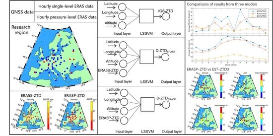
ERA5 data is the fifth-generation global meteorological parameter reanalysis data updated by the European Centre for Medium-Range Weather Forecasts (ECWMF) in January 2019. The ERA5 data is the grid data with a spatial resolution of 0.25° * 0.25° and is provided with one-hour time resolution. It is divided into two types of data, namely the hourly data on single level and the hourly data on pressure levels, both of them can be taken from ECWMF center (https://www.ecmwf.int/en/forecasts/datasets/reanalysis-datasets/era5, accessed on 1 January 2021). The single-level products refer to the meteorological parameters on the surface of Earth. The pressure-level products divide the atmosphere into 37 pressure layers in vertical and provide meteorological parameters on the surface of each pressure layer, which enable ERA5 data to describe changes in meteorological parameters in more detail.
In both types of data, the IGS final product offer ZTD with a temporal resolution of 5 min, while these ZTD values have low spatial resolution owing to the uneven distribution of IGS stations all over the world. Interestingly, the ZTD values can reach a fixed spatial resolution of 0.25° * 0.25° with hourly ERA5 data on a global scale. To unify the temporal resolution of the two types of data, we extract the hourly ZTD values from IGS products, namely IGS-ZTD in this contribution.
2.2. Two Background Data
By using the model method and the integral method, we derive the ZTD values at IGS stations as two background data based on the ERA5 data, namely ERA5S-ZTD and ERA5P-ZTD, respectively. Our specific calculation steps are as follows:
- 1.
- Obtaining original ERA5 data and the position of IGS station. In this study, the ERA5 hourly geopotential (m), 2-meter dewpoint temperature (K), 2-meter temperature (K), surface pressure (Pa) on single-level data, as well as the ERA5 hourly geopotential (m), temperature (K), and specific humidity (%) on 37 pressure-level data are utilized. The latitude, longitude and altitude of the IGS stations are extracted from the tropospheric products.
- 2.
- Getting the WGS84 ellipsoid height. Based on the EGM2008 [25], the ERA5 hourly geopotential of the single-level and the pressure-level products are corrected to ellipsoid height and , respectively.
- 3.
- Deriving meteorological parameters of the IGS stations using the single-level ERA5 data. According to the latitude and longitude of the IGS station, we detect the positions of the four nearest grid points of ERA5 data firstly. Then, the temperature , 2-meter dewpoint , pressure of the IGS stations at the height of are derived through plane interpolation and fitting. Afterwards, these parameters are transformed from the height of to the altitude of the IGS stations. Among them, the altitude difference between and are computed. The corresponding meteorological parameters of the IGS station, , and are derived by the following equations. At last, and the water vapor pressure is calculated using and.where, represents the relative humidity, and the values of , , as well as .
- 4.
- Calculating ERA5S-ZTD by the model method from , and. These meteorological parameters are substituted into the Saastamoinen model [5], and then ERA5S-ZTD values of the IGS stations are obtained using the following equations.where, denotes the latitude of the IGS stations.
- 5.
- Interpolating meteorological parameters above the IGS stations by the pressure-level ERA5 data. According to the relationship of and , the pressure-level data above the IGS stations are retained. Through the plane interpolation and fitting, the temperature and specific humidity of the IGS stations at retained height of are derived. The water vapor pressure is obtained through and.where, is the pressure value of each level.
- 6.
- Calculating ERA5P-ZTD by the integral method. The ERA5P-ZTD values of the IGS stations are obtained by integrating as shown in the following equations [4].where, refers to the atmospheric refractive index at the IGS stations, represents the atmospheric refractive index above the IGS stations, and contains the and in each IGS station. , and are the refractive index constants with the values of 77.604 , 64.79 and 377,600 , respectively.
2.3. Three Schemes Based on the LSSVM Algorithm
2.3.1. LSSVM Algorithm
The training sets (xtrain_i,ytrain_i)i=1,2,3...m and testing sets (xtest_i,ytest_i)i=1,2,3...n are constructed using known data according to the network structure of different schemes, x and y represent the input and output vectors, respectively. The numbers of training sample and testing sample are described as m and n.
For a given training sample (xtrain_i,ytrain_i), the LSSVM algorithm constructs the special function, that is combined with the least-squares equation constraint conditions, to obtain the corresponding Lagrange function equation. The hyper-parameters of optimal model are obtained through the cross-validation method. The optimal solution conditions and the Radial Basis Function (RBF) kernel function matrix K are assembled to compose the LSSVM regression model. These above-mentioned processing is elucidated by the ensuing equations [26].
where, ω represents the weight vector, φ denotes the mapping function, α and are the model parameters, refers to the error vector of the model, refers to the regularization constant, and explains the indicator of the kernel function, which is determined by the cross-validation optimization algorithm. In addition, Table 1 lists the initial parameters and optimization strategy settings of the LSSVM algorithms in this contribution.
2.3.2. Three Schemes
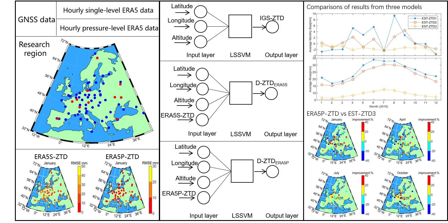
Based on the LSSVM algorithm, we design three schemes to establish the ZTD models according to different background data, namely Scheme 1, Scheme 2, and Scheme 3. The final ZTD estimations of three ZTD models are regarded as EST-ZTD1, EST-ZTD2, and EST-ZTD3 respectively. It should be pointed that, the ZTD data is normalized to [0,1] when the ZTD data is taken as one of input parameters to directly participate in the ZTD modeling based on the LSSVM algorithm, in which the ZTD data includes the IGS-ZTD, the ERA5S-ZTD, as well as ERA5P-ZTD.
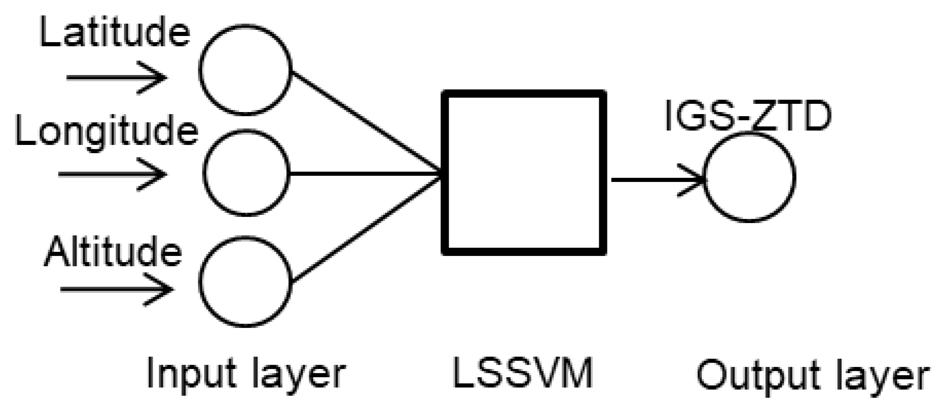
Scheme 1: The core of this scheme is employing the LSSVM algorithm to depict the functional relationship between the station position and the ZTD value, as shown in Figure 1. The input parameters are the longitude, latitude, altitude of the IGS stations, and the output elements are the estimated IGS-ZTD at the corresponding IGS stations. There is no background data involved in the ZTD model. This scheme is also employed in most ZTD models based on machine learning algorithms. When we verify the trained model by testing stations, the EST-ZTD1 at the test station is the output ZTD value of this model.
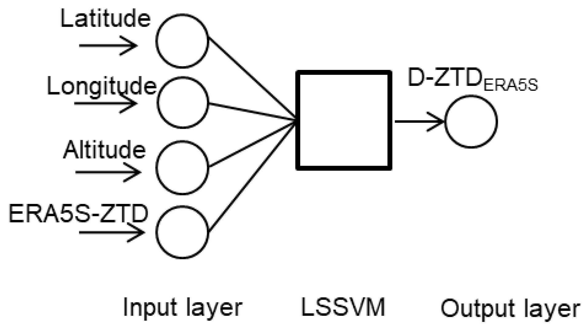
Scheme 2: We introduce the ERA5S-ZTD as background data in the ZTD model. The core of this scheme is to estimate the deviation of ERA5S-ZTD and IGS-ZTD by the LSSVM algorithm, the network structure is shown in Figure 2. In this scheme, the longitude, latitude, altitude, and the ERA5S-ZTD of the IGS station constitute the input vector. The corresponding output parameter is the deviation D-ZTDERA5S depicted through the following equation. In the last, the EST-ZTD2 of the test station is the summation of the estimated D-ZTDERA5S and the corresponding ERA5S-ZTD.
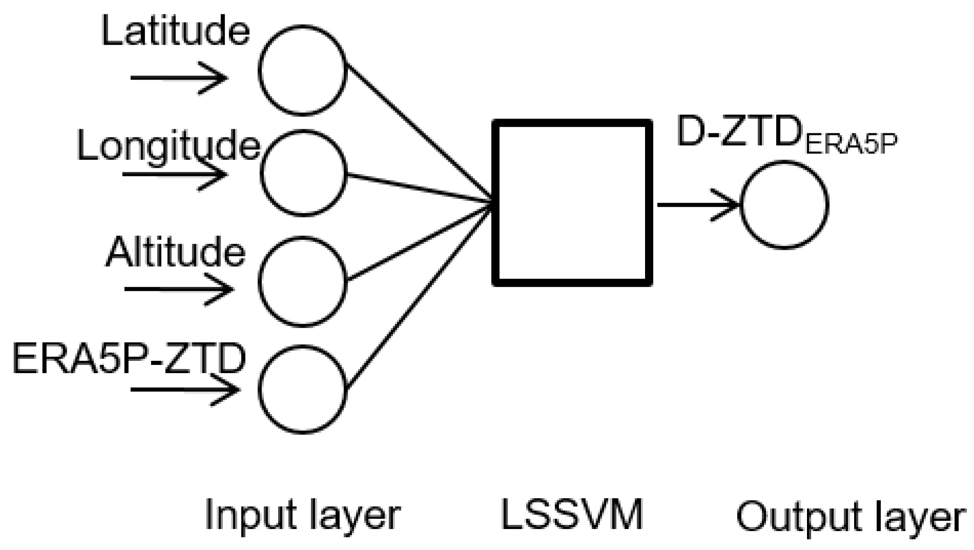
Scheme 3: Similar as Scheme 2, the ERA5P-ZTD replaces the ERA5S-ZTD as the background data in Scheme 3, as shown in the following equation and in Figure 3.
2.4. Accuracy Evaluation
The IGS-ZTD is adopted as the true value because it can reach a high precision of 4 mm. Due to the poor data integrity of some stations in a long time period, we divide the year into 12 months to ensure a sufficient number of samples in the research stage. The monthly bias and the root mean square error (RMSE) of each experimental IGS station are calculated by the following equations. The verifications of three ZTD models are evaluated by the average monthly bias and average RMSE of all testing stations in each month. In addition, piece-wise evaluations of two different background data are performed at each session. The evaluation indexes are the same as that of the ZTD model.
where, is the monthly number of EST-ZTD values for each available station.
3. Results and Analysis
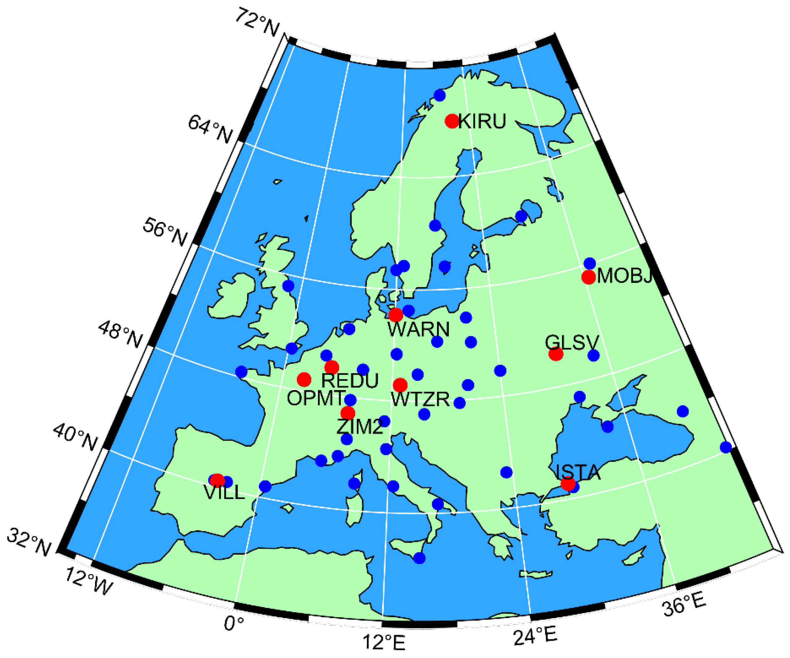
The ERA5 hourly data of the European region (32° N–72° N, 15° W–40° E) in 2018 are extended to the ERA5S-ZTD and the ERA5P-ZTD at the positions of 85 IGS stations. More than 50 IGS stations are available per month, and all of them are employed to investigate the consistency of the extended ERA5S-ZTD and ERA5P-ZTD with IGS-ZTD. Moreover, 10 available IGS stations are selected in each month to verify the accuracy of our three ZTD models, where these models are built by the remaining more than 40 IGS stations derived from the three schemes. Figure 4 displays the distribution of experimental IGS stations in January 2018.
3.1. Accuracy of Two Background ZTD
Table 2 shows the monthly bias and RMSE of the ERA5S-ZTD and ERA5P-ZTD by comparison with the IGS-ZTD at all available stations. For the ERA5S-ZTD, the average bias values are in the range of −2.2–15.7 mm, with the corresponding average RMSE values of 17.4–42.3 mm. Generally, the higher the absolute value of the monthly bias has, the bigger the average RMSE value is. The largest average monthly bias is 15.7 mm with the maximum and minimum values of 68.4 mm and −26.6 mm in August 2018, respectively. Subsequently, the maximum and minimum values of the corresponding RMSE are 18.8 mm and 83.7 mm. For the ERA5P-ZTD, all of the average monthly biases are positive values with the range of 2.1–6.3 mm, and the corresponding average RMSE values are in the range of 7–14.8 mm. Meanwhile, only several RMSE values exceed 20 mm with the maximum RMSE value of 27.1 mm in June 2018.
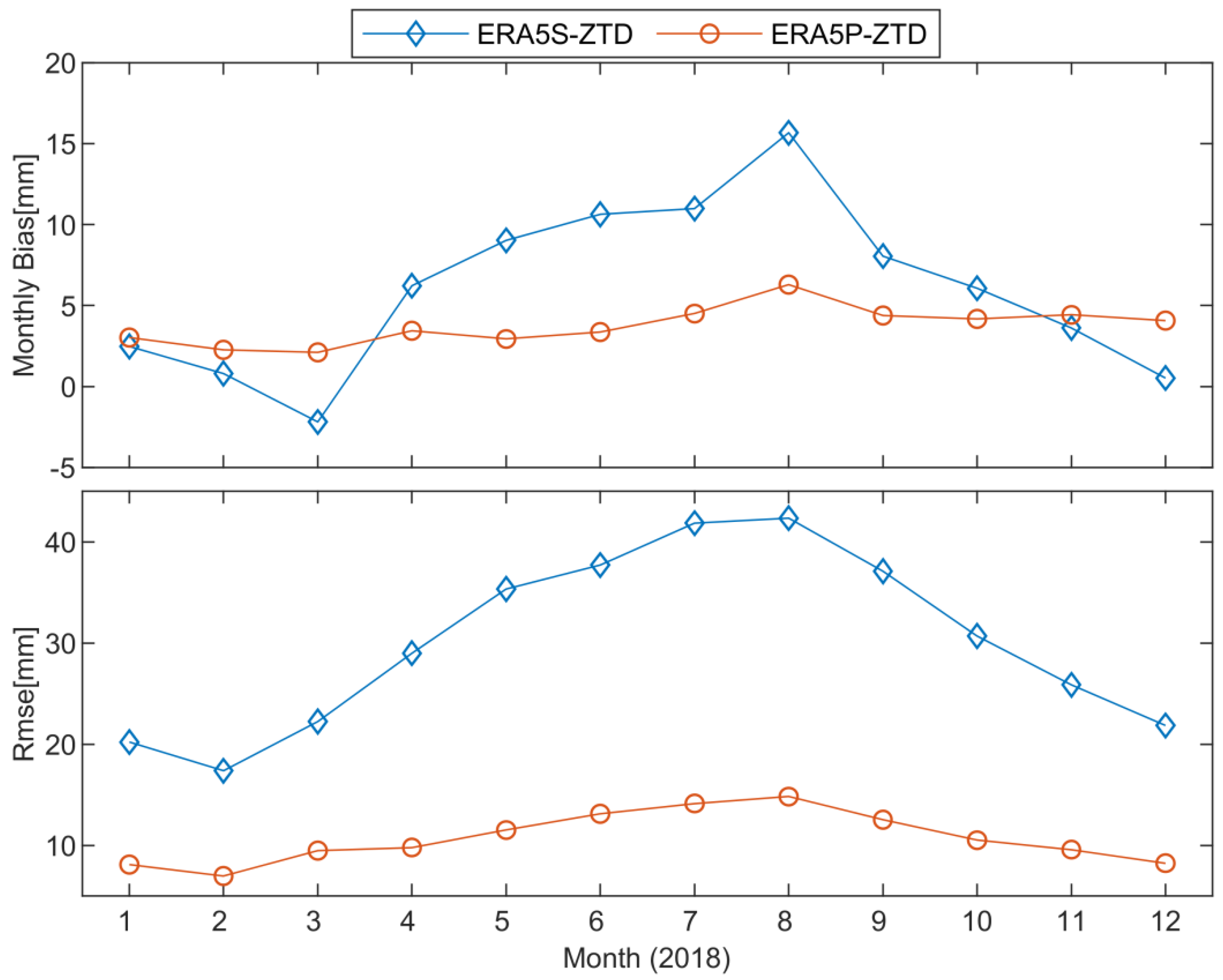
Figure 5 demonstrates the average monthly bias and the average RMSE values of two background ZTD. The average monthly bias of ERA5S-ZTD is larger than that of ERA5P-ZTD from March to October 2018, with the more obvious variation. The average RMSE series of both ERA5S-ZTD and ERA5P-ZTD appear the same trend of rising firstly and then falling over time, and the average RMSE of ERA5S-ZTD is greater than that of ERA5P-ZTD in each month, especially from May to October. These results imply that ERA5S-ZTD has a larger systematic bias with the IGS-ZTD than the ERA5P-ZTD, and the consistency between ERA5P-ZTD and IGS-ZTD are better than that of between ERA5S-ZTD and IGS-ZTD. The reasons are caused by both the difference of the grid data and the processing methods. On one hand, the extended ERA5S-ZTD only uses hourly ERA5 data on the single-level data, while the hourly data on 37 pressure levels are employed in the extended ERA5P-ZTD. On the other hand, the ERA5S-ZTD is obtained by substituting the meteorological parameters into the fixed model, which may have certain system errors, while the ERA5P-ZTD is computed by integrating all the refractive across the path of the GNSS signals.
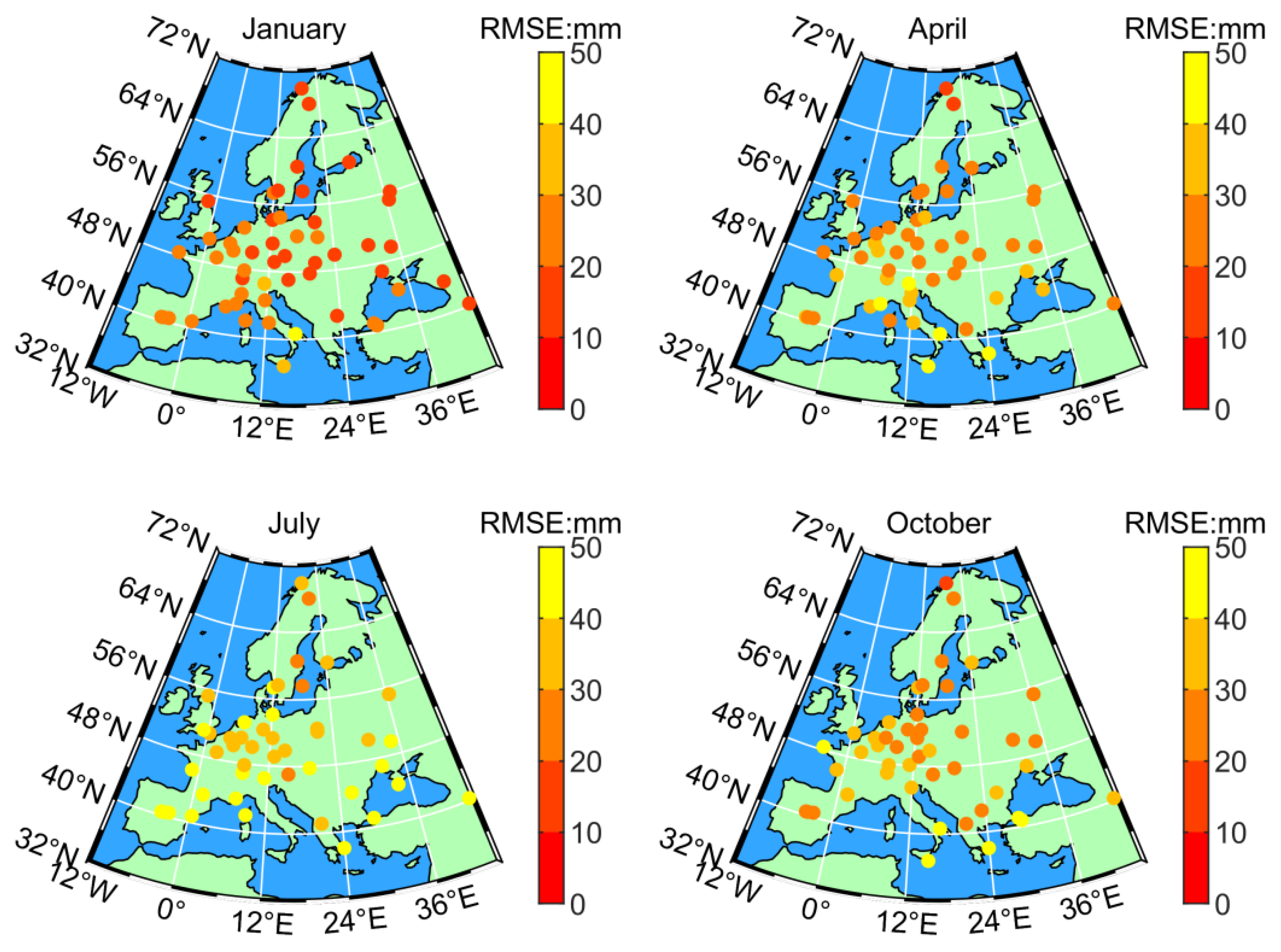
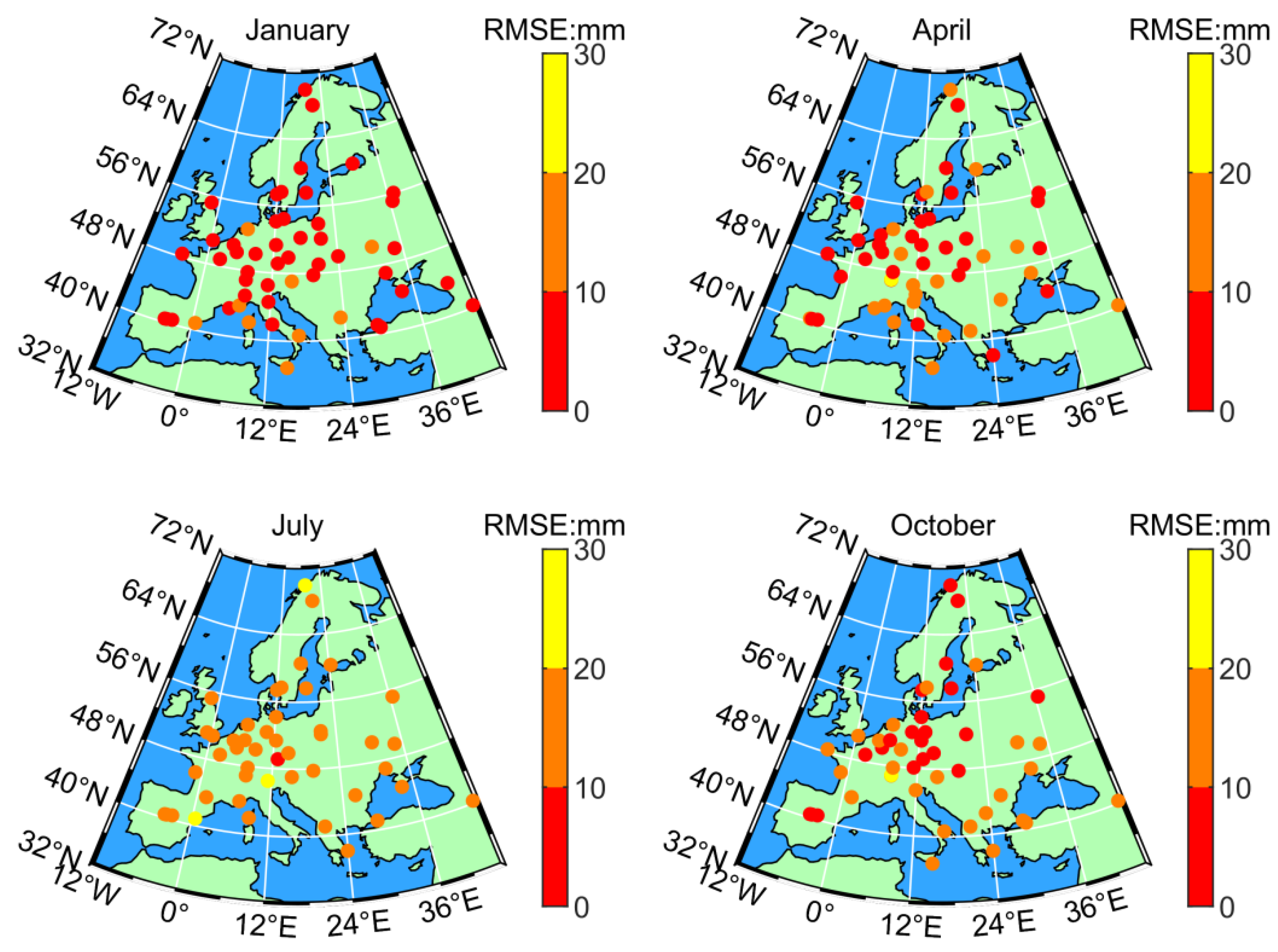
Figure 6 and Figure 7 show the RMSE values of all available IGS stations derived from the ERA5S-ZTD and ERA5P-ZTD in January, April, July, and October of 2018, respectively. This corresponds to winter, spring, summer, and autumn in the northern hemisphere. The RMSE values of each station in January are relatively small for both the ERA5S-ZTD and ERA5P-ZTD, and the highest RMSE appears for these stations in July. This indicates that the situation is a common feature of the whole selected region. The value for tropospheric delay changes with different seasons and latitudes because there are complex meteorological phenomena in the troposphere [27]. In different seasons, the diverse moisture content brings the seasonal variation of the ZTD values. When the summer is coming, the change of the moisture content can get complex and dramatic in a smaller area, while the ability of minor change capturing is limited for the ERA5 grid data. Moreover, the lower RMSE values are always distributed in high latitudes and inland areas, as well as the higher RMSE values mostly appear in low latitudes and coastal regions. It implies that the high heat and active monsoon activities lead to the large and complex ZTD value in low latitudes and coastal areas. The ERA5 data does not indicate this variety of ZTD values perfectly, which brings about this spatial characteristic of RMSE values.
3.2. Accuracy of Three Schemes
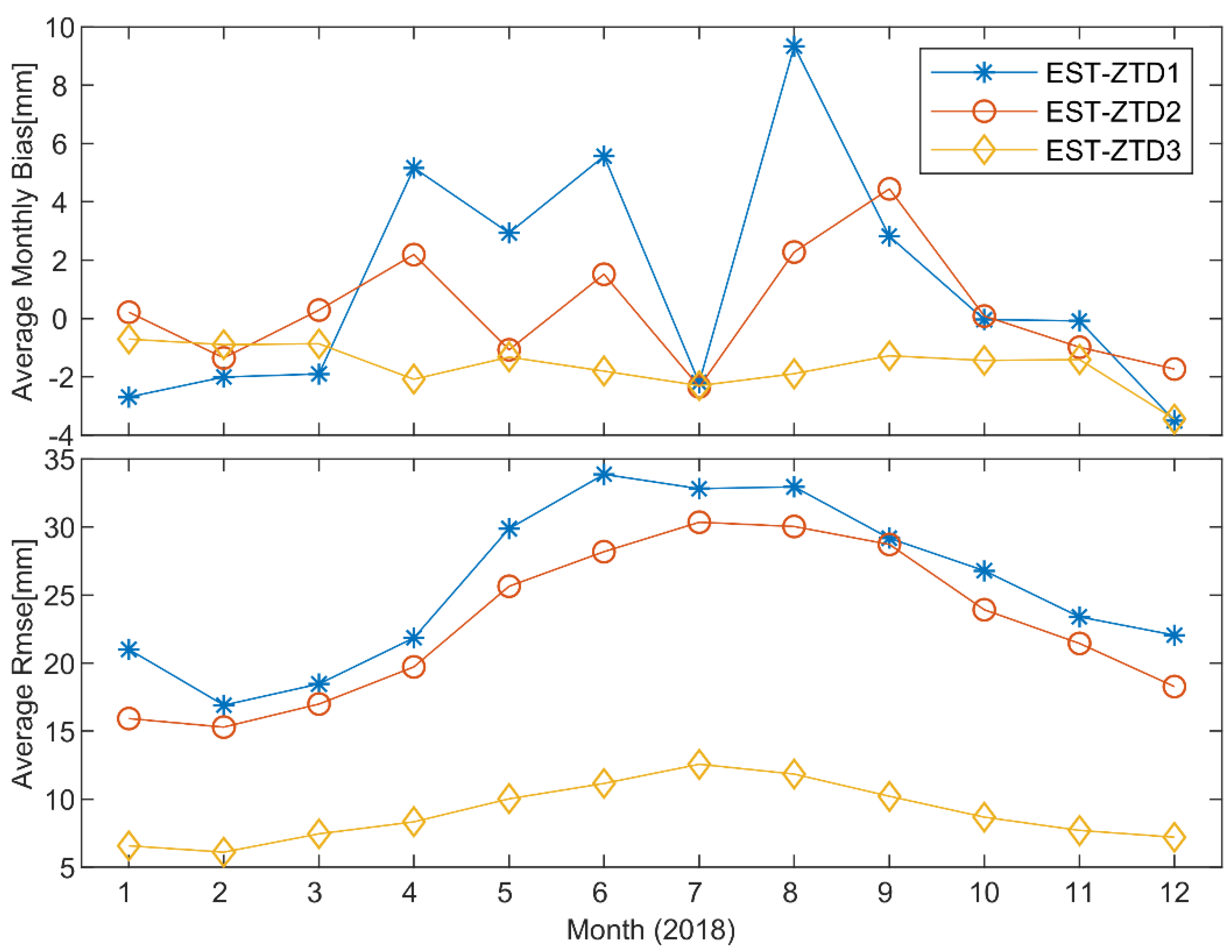
We verify the consistency of our three ZTD models by comparison the estimated ZTD values with IGS-ZTD. Table 3 gives their monthly bias and RMSE values of 10 verification stations. The overall average monthly bias is 1.1 mm, 0.3 mm, and −1.6 mm for Scheme 1, 2, and 3, respectively. The mean value of the average RMSE of 12 months is 25.8 mm, 22.9 mm, and 9.0 mm for Schemes 1, 2, and 3, respectively. Among them, the average monthly bias of 10 verification stations of Scheme 1 is in the range of −3.5–9.3 mm, the corresponding average RMSE values are within 16.9–33.9 mm. The maximum monthly bias of 36.7 mm appears on the individual verification station in August, as well as the maximum RMSE of 52.3 mm. For Scheme 2, the average monthly bias is relatively small with the range of −2.4–4.4 mm in 12 months and the average RMSE is concentrated in the 15.3–30.4 mm. One of 10 verification stations has the maximum monthly bias of 32.4 mm and maximum RMSE value of 54.2 mm in September. In addition, all of the average monthly biases of Scheme 3 are negative values from −0.7 mm to −3.5 mm with the corresponding average RMSE values from 6.1 mm to 12.6 mm.
Figure 8 visualizes the average monthly bias and average RMSE per month. All of the average monthly biases of Scheme 1 and Scheme 2 go up and down around zero in 12 months; that of Scheme 3 is close to zero. These results illustrate that the overall systematic errors are small for all three ZTD models based on the LSSVM algorithm. Interestingly, a near overlap emerges owing to the more negative monthly bias values of three schemes in July 2018. Meanwhile, a temporal feature emerges for the average RMSE values of three ZTD models, where the RMSE values grow in size with the coming of summer. It reflects a common problem that the accumulation of water vapor and the irregular changes of cyclones in summer lead to more difficulty in modeling ZTD. Moreover, the average RMSE values of Scheme 3 and Scheme 2 are smaller than that of Scheme 1, and the value of Scheme 3 is the smallest in each month. It indicates that the two models with extended ERA5 data as background data have a significant advantage compared to the model without background data, and the accuracy of the model based on ERA5P-ZTD is better because the higher consistency occurs between the ERA5P-ZTD and IGS-ZTD.
3.3. Improvement Rate of the Two ZTD Models Based on ERA5S-ZTD and ERA5P-ZTD
To analyze the advantage of the two ZTD models of Scheme 2 and Scheme 3, we compare the RMSE values of the 10 verification stations derived from the two ZTD models with ERA5S-ZTD and ERA5P-ZTD, and their respective improvement rates are calculated according to the following two equations.
where, the RMSEERA5S-ZTD and RMSEERA5P-ZTD refer to the RMSE value of the ERA5S-ZTD and ERA5P-ZTD in each verified station, respectively. The RMSEEST-ZTD2 and RMSEEST-ZTD3 represent the RMSE values of Scheme 2 and Scheme 3 at 10 verification stations.
Table 4 lists the statistical result of the improvement rate based on 10 verification stations. For Scheme 2, the overall average improvement rate reaches 19.1%, with the monthly average improvement rate of from 12.7% to 26.3%. In these months, the optimal improvement rate is up to 61.3% at an individual station in July, as well as the worst rate of −64.7% in June. For Scheme 3, only 1.6% overall average improvement rate is achieved, and most of the monthly average improvement rates are close to zero. During those 12 months, the best monthly average improvement rate is 17.5% with the maximum improvement of 42.5% at one of 10 verification stations in March, and the worst rate is −12.5% with the rate of −86.1% at an individual station in December. By comprehensively comparing the improvement rate of Scheme 2 and Scheme 3, it clearly stands out that the LSSVM algorithm has the excellent performance of compensating the errors derived from ERA5S-ZTD, while the situation is not obvious for the ERA5P-ZTD. Even so, the improvement rate of several stations can also exceed 17% in all 12 months for Scheme 3.
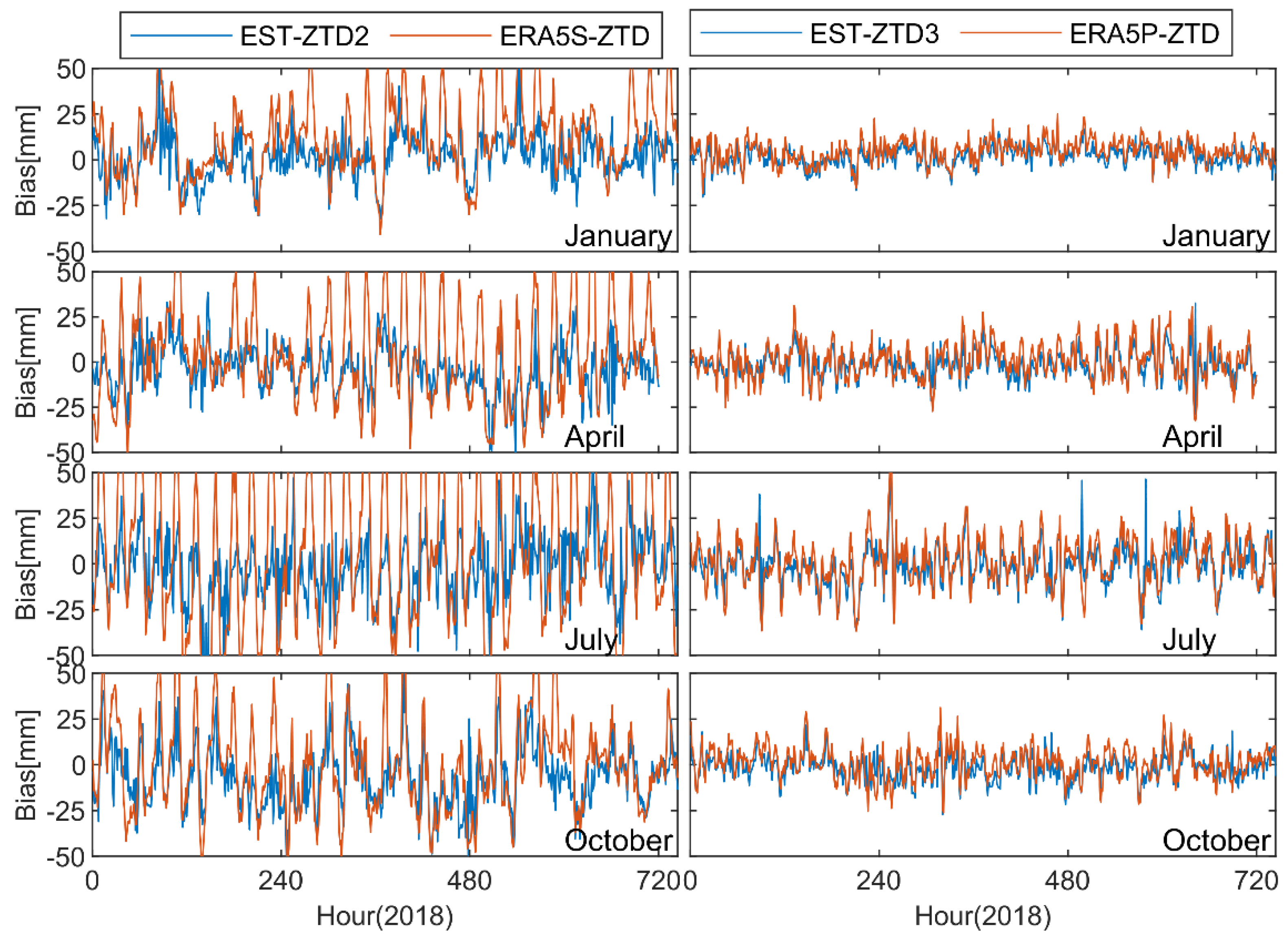
As a typical, Figure 9 and Table 5 display the result of GLSV site in January, April, July, and October of 2018, where the GLSV site is one of the 10 verification stations. Among them, as shown in Figure 9 that significant periodic error signals exist in the bias time series of ERA5S-ZTD and have significantly improved after modeling with ERA5S-ZTD based on the LSSVM algorithm, especially in summer. For the bias time series of ERA5P-ZTD, the periodic error signals have a small fluctuation amplitude compared with ERA5S-ZTD, especially for the results in winter. In addition, the improvement effects from Scheme 3 are not better than that of Scheme 2. As can be seen from the monthly bias in Table 5, EST-ZTD2 model has better correction effect for the obvious systematic errors in ERA5S-ZTD model compared with the improvement of EST-ZTD3 relative to ERA5P-ZTD. Overall, the LSSVM algorithm has better performance in correcting periodic bias of the ERA5S-ZTD, and the extended ERA5P-ZTD by the integral method has good accuracy property, which constrains the improvement capability of the LSSVM algorithm.
4. Discussion
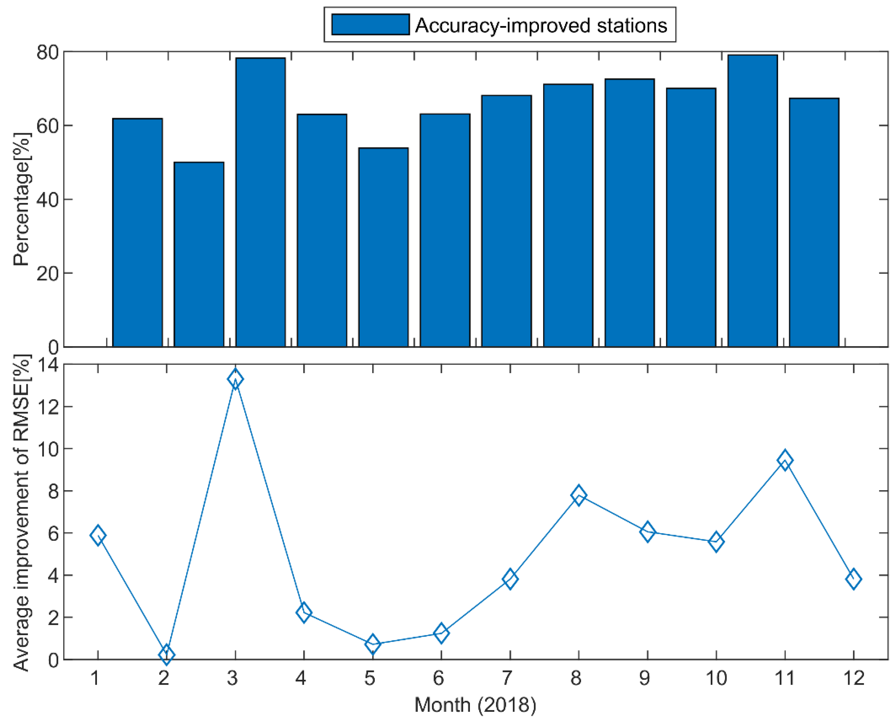
To further investigate the feasibility and availability of the ZTD model of Scheme 3, we perform loop verification on each of the all available IGS stations per month. In each month, each of the available IGS stations is as a testing station in turn to estimate ZTD values, and all remaining available IGS stations are used to train the ZTD model based on the LSSVM algorithm. Afterward, the RMSE values of these estimated ZTD values are evaluated by comparison with IGS-ZTD according to Equation (20), as well as the calculated improvement rate according to Equation (22). We calculate the percentage of all available IGS stations per month by dividing them into the accuracy-improved stations and the accuracy-reduced stations, as well as the overall average improvement rate of their RMSE values. Among them, the percentage of stations with accuracy-reduced stations can be subtracted by the percentage of accuracy-improved stations from 100%. As shown in Figure 10, the percentage of the accuracy-improved stations exceeds 50%, while the overall average improvement rate of RMSE values is less than 10% per month, with the exception of March 2018.
4.1. Dependency of the Estimated ZTD on the Station Distribution
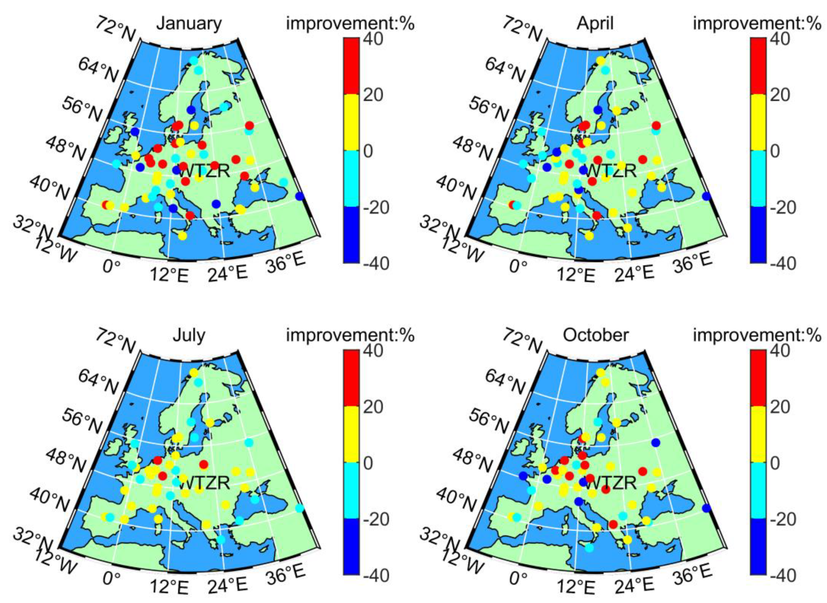
Figure 11 unfolds the improvement rate of each available IGS station in January, April, July, and October of 2018. The most red and yellow spots with the improvement rate in the range of 0–40% are mainly located in the central region of Europe, where the available IGS stations evenly are distributed and compact. This allows that the information of input and output parameters can be comprehensively captured with precision in these areas. The mainly cyan and blue spots with the rate of −40%–0 are located in the edge of the station network or near the coast, and few stations adjacent to them. Therefore, no enough samples can be trained by using the LSSVM algorithm, and the stations located in the coastal area suffer from more drastic climate variability. Specially, several cyan and blue spots are surrounded by a dense network of stations in the central region, such as the WTZR site. It implies that good station distribution is not the unique requirement for the improvement of the estimated ZTD. Therefore, we make a further discussion for the dependency of estimated ZTD on the output parameters D-ZTDERA5P in the next section.
4.2. Dependency of the Estimated ZTD on the Output Parameter D-ZTDERA5P
According to the following formula, we calculate the cosine value of the monthly D-ZTDERA5P time series between the vector of the individual verified station and each of the training station [28].
where, refers to the th training station, denotes the vector of the th training station in the monthly D-ZTDERA5P time series, as well as for the individual verified station. In order to express more clearly the similarity of the training samples with the verified sample, we give the average-cosine value as
where refers to the number of training stations in each month.
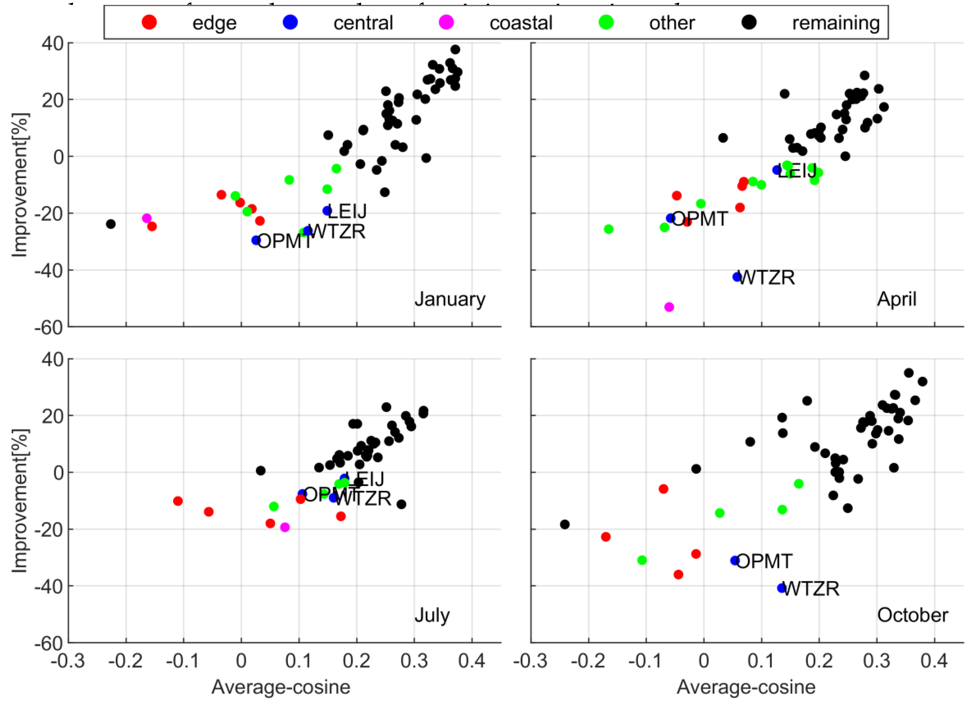
In Figure 12, we divide the available IGS station in January, April, July, and October of 2018 according to the station distribution, the improvement rate , as well as . When , the similarity of the training samples with the verified samples is weak. The overall trend between the average-cosine and the improvement rate tends to be linear from black spots, where the improvement rate increases with the rise of the average-cosine value. The average-cosine values of most stations are more than 0.2 with a positive improvement rate. It implies that the overall accuracy of estimated ZTD from Scheme 3 is superior to the accuracy of ERA5P-ZTD. Moreover, the overall improved accuracy is associated with the similarity between training stations and testing stations.
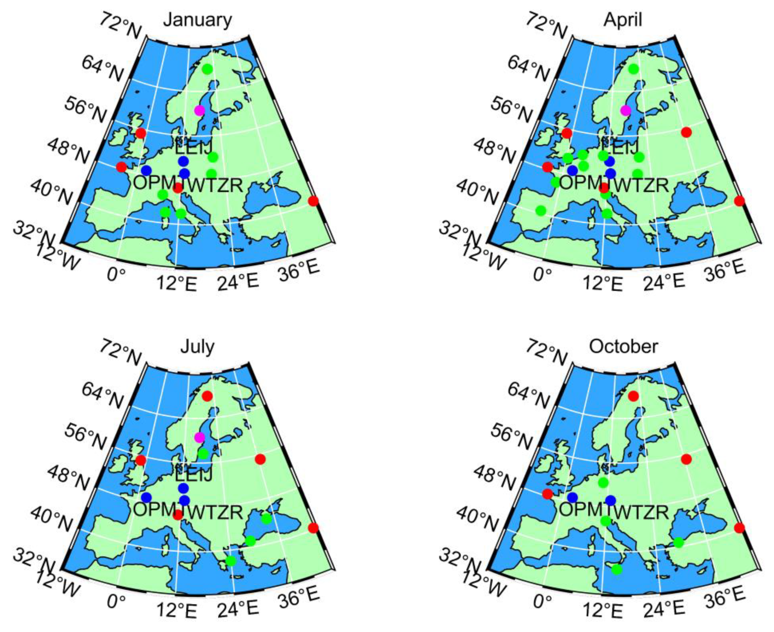
Although the WTZR, OPMT, and LEIJ sites with blue spots are surrounded by a dense network of stations in the central region as shown in Figure 13, their average-cosine values are less than 0.2 at least three months in January, April, July, and October of 2018. The estimated ZTD values of the three sites have a negative improvement rate owing to the trained stations have lower similarity with them. For the sites with red, magenta, and green spots, they are always located on the edge of the region or near the coast. On one hand, their locations are relatively outliers when their ZTDs are estimated, which also leads to a lower similarity and negative improvement rate. On the other hand, the large change of air humidity often occurs near the coast, and the accuracy of ZTD modeling become unstable owing to the influence of the abundant water vapor and active monsoon climate. Overall, this is a common problem for the ZTD modeling. Even though, the improvement rate of estimated ZTD is positive for most stations, and the biggest improvement rate from Scheme 3 can reach about 40%.
5. Conclusions
As a fresh meteorological reanalysis data, the ERA5 data has higher spatial resolution than the IGS-ZTD. In addition, the LSSVM algorithm has a more stable computing performance than the traditional BPNN algorithm. In this paper, we combine the ERA5 data with IGS-ZTD by using the LSSVM algorithm. Among them, we extend the ERA5 data to ERA5S-ZTD and ERA5P-ZTD based on the model method and integral method, and design three schemes to build ZTD models.
The consistency of ERA5P-ZTD with IGS-ZTD is better than that of ERA5S-ZTD owing to the integral method, as well as the multiple pressure-level data. The overall average RMSE value is 30.1 mm and 10.7 mm for ERA5S-ZTD and ERA5P-ZTD, respectively. While they have the same trend with the seasonal variation, the RMSE values reach biggest with the coming of summer. In addition, the stations located in low latitudes and coastal regions have always higher RMSE values owing to the high heat and active monsoon activities.
For the three ZTD models, the overall average monthly bias is 1.1 mm, 0.3 mm, and −1.6 mm, with the corresponding mean value of average RMSE values of 25.8 mm, 22.9 mm, and 9.0 mm for Schemes 1, 2, and 3, respectively. Hardly any systematic errors exist for all three ZTD models based on the LSSVM algorithm, and the ZTD modeling accuracy is significantly improved when the ERA5 data is added, especially for the ZTD model with ERA5P-ZTD. Meanwhile, the seasonal characteristics still exist owing to the accumulation of water vapor and the irregular changes of cyclones in summer, as well as the accuracy limitation of ERA5S-ZTD and ERA5P-ZTD.
To investigate the advantage of the combination of ERA5 data using the LSSVM algorithm, the improvement rates are analyzed and discussed in detail. The overall improvement rate has 19.1% for the ZTD model with ERA5S-ZTD, and 1.6% for the ZTD model with ERA5P-ZTD. The LSSVM algorithm shows excellent performance in correcting systematic and periodic errors of ERA5S-ZTD, while the overall improvement effect is weak for the ZTD model with ERA5P-ZTD.
Moreover, we perform loop verification of each available IGS station to explore the reason for the lower improvement for the ZTD model with ERA5P-ZTD. The dependency of estimated ZTD on the station distribution and the output parameters D-ZTDERA5P are discussed. On one hand, the improvement rate is positive for most stations located in the central region of the regional network, and the biggest monthly improvement rate can even reach about 40%. On the other hand, the improvement rate is negative for several stations. They are always located on the edge of the region, or near the coast. Additionally, they suffer from both the scare training samples and more drastic climate variability around them. Furthermore, a few stations are surrounded by a dense network of stations in the central region with a negative improvement rate, which is mainly caused by the lower similarity between the individual verified station and training stations. Overall, the two discussed dependencies are the common problem for the ZTD modeling, and it is important to refine the strategies of multisource combination based on the excellent machine learning algorithms in the near future.
Author Contributions
Conceptualization, T.X.; methodology, S.L.; software, S.L.; validation, T.X., N.J. and H.Y.; formal analysis, S.L. and H.Y.; investigation, S.L., S.W. and Z.Z.; resources, T.X.; data curation, S.L.; writing—original draft preparation, S.L.; writing—review and editing, S.L., T.X., N.J. and H.Y.; visualization, S.L. and H.Y.; supervision, T.X. and H.Y.; project administration, T.X.; funding acquisition, T.X. All authors have read and agreed to the published version of the manuscript.
Funding
This study is financially supported by the National Key Research & Development Program of China (2020YFB0505800, and 2020YFB0505804), the National Natural Science Foundation of China (41874032) and Natural Science Foundation of Shandong Province, China (ZR2020QD046 and ZR2020MD045).
Institutional Review Board Statement
Not applicable.
Informed Consent Statement
Informed consent was obtained from all subjects involved in the study.
Data Availability Statement
Not applicable.
Acknowledgments
The authors would like to extend their sincere gratitude to ECMWF and IGS for providing the relevant data.
Conflicts of Interest
The authors declare no conflict of interest.
References
- Rocken, C.; Ware, R.; Van Hove, T.; Solheim, F.; Alber, C.; Johnson, J.; Bevis, M.; Businger, S. Sensing atmospheric water vapor with the global positioning system. Geophys. Res. Lett. 1993, 20, 2631–2634. [Google Scholar] [CrossRef] [Green Version]
- Bevis, M.; Businger, S.; Chiswell, S.; Herring, T.A.; Anthes, R.A.; Rocken, C.; Ware, R.H. GPS Meteorology: Mapping Zenith Wet Delays onto Precipitable Water. J. Appl. Meteorol. 1994, 33, 379–386. [Google Scholar] [CrossRef]
- Davis, J.L.; Herring, T.A.; Shapiro, I.I.; Rogers, A.E.E.; Elgered, G. Geodesy by radio interferometry: Effects of atmospheric modeling errors on estimates of baseline length. Radio Sci. 1985, 20, 1593–1607. [Google Scholar] [CrossRef]
- Askne, J.; Nordius, H. estimation of tropospheric delay for microwaves from surface weather data. Radio Sci. 1987, 22, 379–386. [Google Scholar] [CrossRef]
- Saastamoinen, J. Atmospheric Correction for the Troposphere and Stratosphere in Radio Ranging Satellites. In Use of Aritificial Satellites for Geodesy; Wiley: Hoboken, NJ, USA, 1972; Volume 15, pp. 247–251. [Google Scholar]
- Hopfield, H.S. Two-quartic tropospheric refractivity profile for correcting satellite data. J. Geophys. Res. 1969, 74, 4487–4499. [Google Scholar] [CrossRef]
- Collins, J.P.; Langley, R.B. The residual tropospheric propagation delay: How bad can it get? In Proceedings of the Proc. ON GPS 1998, 11th International Technical Meeting of the Satellite Division of the Institute of Navigation, Nashville, TN, USA, 15–18 September 1998; pp. 729–738. [Google Scholar]
- Penna, N.; Dodson, A.; Chen, W. Assessment of EGNOS tropospheric correction model. J. Navig. 2001, 54, 37–55. [Google Scholar] [CrossRef] [Green Version]
- Boehm, J.; Heinkelmann, R.; Schuh, H. Short Note: A global model of pressure and temperature for geodetic applications. J. Geod. 2007, 81, 679–683. [Google Scholar] [CrossRef]
- Lagler, K.; Schindelegger, M.; Bohm, J.; Krasna, H.; Nilsson, T. GPT2: Empirical slant delay model for radio space geodetic techniques. Geophys. Res. Lett. 2013, 40, 1069–1073. [Google Scholar] [CrossRef] [PubMed] [Green Version]
- Landskron, D.; Bohm, J. VMF3/GPT3: Refined discrete and empirical troposphere mapping functions. J. Geod. 2018, 92, 349–360. [Google Scholar] [CrossRef]
- Wang, S.; Xu, T.; Nie, W.; Jiang, C.; Yang, Y.; Fang, Z.; Li, M.; Zhang, Z. Evaluation of Precipitable Water Vapor from Five Reanalysis Products with Ground-Based GNSS Observations. Remote Sens. 2020, 12, 1817. [Google Scholar] [CrossRef]
- Ding, M. A neural network model for predicting weighted mean temperature. J. Geod. 2018, 92, 1187–1198. [Google Scholar] [CrossRef]
- Ding, M. A second generation of the neural network model for predicting weighted mean temperature. GPS Solut. 2020, 24, 61. [Google Scholar] [CrossRef]
- Benevides, P.; Catalao, J.; Nico, G. Neural Network Approach to Forecast Hourly Intense Rainfall Using GNSS Precipitable Water Vapor and Meteorological Sensors. Remote Sens. 2019, 11, 966. [Google Scholar] [CrossRef] [Green Version]
- Pan, Y.; Ren, C.; Liang, Y.; Zhang, Z.; Shi, Y. Inversion of surface vegetation water content based on GNSS-IR and MODIS data fusion. Satell. Navig. 2020, 1. [Google Scholar] [CrossRef]
- Katsougiannopoulos, S.; Pikridas, C. Prediction of zenith tropospheric delay by multi-layer perceptron. J. Appl. Geod. 2009, 3, 223–229. [Google Scholar] [CrossRef]
- Suparta, W.; Alhasa, K.M. Application of ANFIS Model for Prediction of Zenith Tropospheric Delay. In Proceedings of the 2013 3rd International Conference on Instrumentation, Communications, Information Technology, and Biomedical Engineering (ICICI-BME), Bandung, Indonesia, 7–8 November 2013; pp. 172–177. [Google Scholar]
- Suparta, W.; Alhasa, K.M. Modeling of Tropospheric Delays Using ANFIS; Springer: Berlin/Heidelberg, Germany, 2016. [Google Scholar] [CrossRef]
- Xiao, G.W.; Ou, J.K.; Liu, G.L.; Zhang, H.X. Construction of a regional precise tropospheric delay model based on improved BP neural network. Chin. J. Geophys. Chin. Ed. 2018, 61, 3139–3148. [Google Scholar] [CrossRef]
- Zhang, Q.; Li, F.; Zhang, S.; Li, W. Modeling and Forecasting the GPS Zenith Troposphere Delay in West Antarctica Based on Different Blind Source Separation Methods and Deep Learning. Sensors 2020, 20, 2343. [Google Scholar] [CrossRef] [PubMed] [Green Version]
- Albergel, C.; Dutra, E.; Munier, S.; Calvet, J.-C.; Munoz-Sabater, J.; de Rosnay, P.; Balsamo, G. ERA-5 and ERA-Interim driven ISBA land surface model simulations: Which one performs better? Hydrol. Earth Syst. Sci. 2018, 22, 3515–3532. [Google Scholar] [CrossRef] [Green Version]
- Sun, Z.; Zhang, B.; Yao, Y. An ERA5-Based Model for Estimating Tropospheric Delay and Weighted Mean Temperature Over China With Improved Spatiotemporal Resolutions. Earth Space Sci. 2019, 6, 1926–1941. [Google Scholar] [CrossRef]
- Jiang, C.; Xu, T.; Wang, S.; Nie, W.; Sun, Z. Evaluation of Zenith Tropospheric Delay Derived from ERA5 Data over China Using GNSS Observations. Remote Sens. 2020, 12, 663. [Google Scholar] [CrossRef] [Green Version]
- Pavlis, N.K.; Holmes, S.A.; Kenyon, S.C.; Factor, J.K. The development and evaluation of the Earth Gravitational Model 2008 (EGM2008). J. Geophys. Res. Solid Earth 2012, 117. [Google Scholar] [CrossRef] [Green Version]
- Suykens, J.A.K.; Vandewalle, J. Least squares support vector machine classifiers. Neural Process. Lett. 1999, 9, 293–300. [Google Scholar] [CrossRef]
- Li, R.; Zheng, S.; Wang, E.; Chen, J.; Feng, S.; Wang, D.; Dai, L. Advances in BeiDou Navigation Satellite System (BDS) and satellite navigation augmentation technologies. Satell. Navig. 2020, 1. [Google Scholar] [CrossRef]
- Kima, M.-C.; Choi, K.-S. A comparison of collocation-based similarity measures in query expansion. Inf. Process. Manag. 1999, 35, 19–30. [Google Scholar] [CrossRef]
Figure 1.
Network structure of Schemes 1.

Figure 2.
Network structure of Scheme 2.

Figure 3.
Network structure of Scheme 3.

Figure 4.
Distribution of experimental IGS stations in January 2018. Blue spots represent the training sites, and 10 testing sites are shown by red points.
Figure 4.
Distribution of experimental IGS stations in January 2018. Blue spots represent the training sites, and 10 testing sites are shown by red points.

Figure 5.
Average monthly bias and average RMSE of ERA5S-ZTD and ERA5P-ZTD in 2018.

Figure 6.
RMSE values of ERA5S-ZTD at all available IGS stations in January, April, July, and October of 2018. These RMSE values of ERA5S-ZTD are concentrating in the range of 25–50 mm.
Figure 6.
RMSE values of ERA5S-ZTD at all available IGS stations in January, April, July, and October of 2018. These RMSE values of ERA5S-ZTD are concentrating in the range of 25–50 mm.

Figure 7.
RMSE values of ERA5P-ZTD at all available IGS stations in January, April, July, and October of 2018. These RMSE values of ERA5P-ZTD are always less than 20 mm.
Figure 7.
RMSE values of ERA5P-ZTD at all available IGS stations in January, April, July, and October of 2018. These RMSE values of ERA5P-ZTD are always less than 20 mm.

Figure 8.
Average monthly bias and average RMSE of estimated ZTD values at 10 verifying IGS stations based on the three schemes.
Figure 8.
Average monthly bias and average RMSE of estimated ZTD values at 10 verifying IGS stations based on the three schemes.

Figure 9.
Bias time series of ZTD estimations at the GLSV site in January, April, July, and October of 2018. The four subgraphs on the left refer to the bias time series from ERA5S-ZTD and Scheme 2, and four subgraphs on the right for the ERA5P-ZTD and Scheme 3.
Figure 9.
Bias time series of ZTD estimations at the GLSV site in January, April, July, and October of 2018. The four subgraphs on the left refer to the bias time series from ERA5S-ZTD and Scheme 2, and four subgraphs on the right for the ERA5P-ZTD and Scheme 3.

Figure 10.
Statistical improvements of Scheme 3 at all stations. The up sub-figure depicts the proportion of accuracy-improved stations. The average improvement of RMSE at all stations is shown in the down subfigure.
Figure 10.
Statistical improvements of Scheme 3 at all stations. The up sub-figure depicts the proportion of accuracy-improved stations. The average improvement of RMSE at all stations is shown in the down subfigure.

Figure 11.
Distribution of improvement rate of all available stations from Scheme 3 in January, April, July, and October of 2018. Red spots refer to the improvement rate of the available IGS stations in the range of 0–20%, 20%–40% for yellow spots, −20%–0 for cyan spots, and −40%–−20% for blue spots.

Figure 12.
Similarity of the improvement rate with average-cosine value for each available station in January, April, July, and October of 2018. Among them, the black spots refer to the station with the improvement rate or . The red spots refer to the stations located in the edge region with the improvement rate and , the blue spots for the stations located in the central region, and the magenta spots for the stations close to the coast. For the red, blue, and magenta spots, their corresponding stations are included at least three months in January, April, July, and October of 2018. The other stations are presented by using the green spots.

Figure 13.
Station distribution based on the conditions of improvement rate , and . These spots with different color correspond with the colored spots in Figure 12.
Figure 13.
Station distribution based on the conditions of improvement rate , and . These spots with different color correspond with the colored spots in Figure 12.


Table 1.
Initial parameters setting of the LSSVM algorithm.
| Parameter Name | Value |
|---|---|
| C | 10,000 |
| 2 | |
| type | ‘function estimation’ |
| kernel | ‘RBF_kernel’ |
| preprocess | ‘preprocess’ |
| Method of optimization | ‘grid search’ |
| Method of testing | ‘crossvalidatalssvm’ |
Table 2.
Monthly bias and RMSE of the ERA5S-ZTD and ERA5P-ZTD by comparison with the IGS-ZTD at all available stations. Values in brackets refer to the monthly minimal and maximal value for all available stations. Unit is millimeter.
Table 2.
Monthly bias and RMSE of the ERA5S-ZTD and ERA5P-ZTD by comparison with the IGS-ZTD at all available stations. Values in brackets refer to the monthly minimal and maximal value for all available stations. Unit is millimeter.
| ERA5S-ZTD | ERA5P-ZTD | |||
|---|---|---|---|---|
| Monthly Bias | RMSE | Monthly Bias | RMSE | |
| January | 2.5 [−29.6,32.9] | 20.2 [10.4,41.1] | 3.0 [−9.6,12.8] | 8.1 [4.6,17.1] |
| February | 0.8 [−16.3,25.6] | 17.4 [8.4,30.6] | 2.3 [−14.7,11.8] | 7.0 [3.4,14.0] |
| March | −2.2 [−26.7,15.0] | 22.2 [7.2,36.5] | 2.1 [−12.2,17.8] | 9.5 [4.9,19.7] |
| April | 6.2 [−37.0,42.3] | 29.0 [10.6,54.7] | 3.5 [−10.4,21.8] | 9.8 [4.7,23.2] |
| May | 9.0 [−53.7,40.4] | 35.3 [23.0,60.2] | 2.9 [−14.1,19.5] | 11.5 [6.7,22.0] |
| June | 10.6 [−13.9,39.1] | 37.7 [15.1,68.1] | 3.4 [−11.9,24.0] | 13.1 [5.9,27.1] |
| July | 11.0 [−7.5,62.0] | 41.8 [26.0,81.3] | 4.5 [−12.9,18.7] | 14.1 [10.0,23.9] |
| August | 15.7 [−26.6,68.4] | 42.3 [18.8,83.7] | 6.3 [−12.9,21.8] | 14.8 [6.9,26.1] |
| September | 8.1 [−49.1,52.7] | 37.1 [7.3,66.4] | 4.4 [−9.1,21.7] | 12.5 [7.8,24.3] |
| October | 6.1 [−23.3,35.6] | 30.7 [16.9,46.6] | 4.2 [−8.3,24.3] | 10.5 [6.2,25.8] |
| November | 3.6 [−24.0,37.3] | 25.9 [16.5,46.7] | 4.4 [−10.8,12.5] | 9.6 [5.6,17.0] |
| December | 0.5 [−17.7,20.1] | 21.9 [14.4,33.3] | 4.1 [−2.9,21.3] | 8.2 [4.2,22.3] |
| Mean | 6.0 | 30.1 | 3.8 | 10.7 |
Table 3.
Monthly bias and RMSE values of 10 verification stations. Values in brackets refer to the monthly minimal and maximal value for 10 verifying stations. Unit is millimeter.
Table 3.
Monthly bias and RMSE values of 10 verification stations. Values in brackets refer to the monthly minimal and maximal value for 10 verifying stations. Unit is millimeter.
| EST-ZTD1 | EST-ZTD2 | EST-ZTD3 | ||||
|---|---|---|---|---|---|---|
| Monthly Bias | RMSE | Monthly Bias | RMSE | Monthly Bias | RMSE | |
| January | −2.7 [−17.7,8.9] | 21.0 [12.1,33.0] | 0.2 [−10.0,11.1] | 15.9 [9.4,21.5] | −0.7 [−6.8,5.9] | 6.6 [4.4,9.4] |
| February | −2.0 [−20.6,4.0] | 16.9 [7.9,35.1] | −1.3 [−13.6,8.3] | 15.3 [9.5,27.8] | −0.9 [−6.4,5.2] | 6.1 [4.0,8.1] |
| March | −1.9 [−12.3,13.3] | 18.5 [9.5,29.1] | 0.3 [−6.9,9.1] | 17 [8.0,27.0] | −0.9 [−6.5,5.1] | 7.4 [5.2,9.6] |
| April | 5.2 [−4.7,26.6] | 21.9 [9.7,36.6] | 2.2 [−5.7,21.0] | 19.7 [8.6,33.1] | −2.1 [−8.5,5.5] | 8.3 [5.2,11.4] |
| May | 2.9 [−10.9,17.1] | 29.9 [18.5,48.7] | −1.1 [−17.5,20.7] | 25.7 [17,35] | −1.3 [−7.5,5.9] | 10 [8.5,12.2] |
| June | 5.6 [−9.1,27.5] | 33.9 [20,48.2] | 1.5 [−8,17.1] | 28.2 [18,46] | −1.8 [−6.6,2.3] | 11.1 [8.5,13.2] |
| July | −2.2 [−15.8,15.6] | 32.8 [22.2,49.1] | −2.4 [−16.9,9.9] | 30.4 [18.2,43.7] | −2.3 [−7.9,2.6] | 12.6 [10.9,14.0] |
| August | 9.3 [−11.2,36.7] | 33 [22.8,52.3] | 2.3 [−9.7,28.5] | 30 [17.4,44.2] | −1.9 [−7.6,2.5] | 11.8 [7.3,14.9] |
| September | 2.8 [−14.4,13.6] | 29.2 [15.7,48.9] | 4.4 [−8.6,32.4] | 28.7 [13.4,54.2] | −1.3 [−6.2,6.4] | 10.2 [6.7,13.1] |
| October | 0 [−11.0,3.9] | 26.8 [14.0,40.5] | 0.1 [−12.6,15.3] | 23.9 [15.2,35.5] | −1.4 [−7.2,6.3] | 8.7 [6.5,10.7] |
| November | −0.1 [−9.8,7.9] | 23.4 [10.0.40.4] | −1 [−9.2,16.8] | 21.5 [13.4,42.8] | −1.4 [−6.4,7.0] | 7.7 [5.8,10.3] |
| December | −3.5 [−21.3,15.3] | 22.1 [9.7,31.3] | −1.7 [−9.5,7.3] | 18.3 [11.7,23.8] | −3.5 [−7.9,0.5] | 7.2 [5.1,9.1] |
| Mean | 1.1 | 25.8 | 0.3 | 22.9 | −1.6 | 9.0 |
Table 4.
Improvement rate of Schemes 2 and 3. Values in brackets refer to the monthly minimal and maximal improvement rate for 10 verifying stations. Unit is percent.
Table 4.
Improvement rate of Schemes 2 and 3. Values in brackets refer to the monthly minimal and maximal improvement rate for 10 verifying stations. Unit is percent.
| Improvement- Scheme 2 | Improvement- Scheme 3 | |
|---|---|---|
| January | 18.8 [−0.1,48.8] | 7.4 [−31.4,37.3] |
| February | 12.7 [−19.9,36.4] | −0.2 [−35.2,35.1] |
| March | 20.7 [−10.0,43.3] | 17.5 [−11.2,42.5] |
| April | 26.3 [2.5,50.7] | −0.9 [−44.8,22.5] |
| May | 16.8 [−50.0,48.1] | −2.2 [−32.3,19.0] |
| June | 16.4 [−64.7,45.5] | −0.2 [−44.1,22.3] |
| July | 18.2 [−28.4,61.3] | −1.8 [−19.6,17.7] |
| August | 23.9 [−10.8,46.3] | 0.6 [−29.4,25.1] |
| September | 23.4 [−1.4,46.2] | 5.3 [−19.6,23.4] |
| October | 20.6 [−33.8,46.2] | 0.4 [−32.3,28.9] |
| November | 17.8 [−3.3,45.3] | 5.5 [−21.6,38.6] |
| December | 13.4 [−20.4,49.8] | −12.5 [−86.1,33.8] |
| Mean | 19.1 | 1.6 |
Table 5.
Monthly bias and RMSE of ZTD estimations from ERA5S-ZTD, EST-ZTD2, ERA5P-ZTD and EST-ZTD3 model at the GLSV site in January, April, July, and October of 2018. Unit is millimeters.
Table 5.
Monthly bias and RMSE of ZTD estimations from ERA5S-ZTD, EST-ZTD2, ERA5P-ZTD and EST-ZTD3 model at the GLSV site in January, April, July, and October of 2018. Unit is millimeters.
| ERA5S-ZTD | EST-ZTD2 | ERA5P-ZTD | EST-ZTD3 | |||||
|---|---|---|---|---|---|---|---|---|
| Monthly Bias | RMSE | Monthly Bias | RMSE | Monthly Bias | RMSE | Monthly Bias | RMSE | |
| January | −12.7 | 24.3 | 1.7 | 12.4 | −4.7 | 7.8 | 2.1 | 5.8 |
| April | −5.5 | 28.8 | −4.4 | 14.2 | −0.7 | 9.8 | −1.4 | 7.7 |
| July | −10.1 | 47.0 | −2.2 | 18.2 | −1.3 | 13.0 | −0.8 | 10.9 |
| October | −0.7 | 27.4 | −6.8 | 18.2 | −1.1 | 8.6 | −1.7 | 7.2 |
Publisher’s Note: MDPI stays neutral with regard to jurisdictional claims in published maps and institutional affiliations. |
© 2021 by the authors. Licensee MDPI, Basel, Switzerland. This article is an open access article distributed under the terms and conditions of the Creative Commons Attribution (CC BY) license (http://creativecommons.org/licenses/by/4.0/).
Share and Cite
MDPI and ACS Style
Li, S.; Xu, T.; Jiang, N.; Yang, H.; Wang, S.; Zhang, Z. Regional Zenith Tropospheric Delay Modeling Based on Least Squares Support Vector Machine Using GNSS and ERA5 Data. Remote Sens. 2021, 13, 1004. https://doi.org/10.3390/rs13051004
AMA Style
Li S, Xu T, Jiang N, Yang H, Wang S, Zhang Z. Regional Zenith Tropospheric Delay Modeling Based on Least Squares Support Vector Machine Using GNSS and ERA5 Data. Remote Sensing. 2021; 13(5):1004. https://doi.org/10.3390/rs13051004
Chicago/Turabian StyleLi, Song, Tianhe Xu, Nan Jiang, Honglei Yang, Shuaimin Wang, and Zhen Zhang. 2021. "Regional Zenith Tropospheric Delay Modeling Based on Least Squares Support Vector Machine Using GNSS and ERA5 Data" Remote Sensing 13, no. 5: 1004. https://doi.org/10.3390/rs13051004
Note that from the first issue of 2016, this journal uses article numbers instead of page numbers. See further details here.