
Retrieval of Daytime Total Column Water Vapour from OLCI Measurements over Land Surfaces


Institute for Space Sciences, Freie Universität Berlin (FUB), Carl-Heinrich-Becker-Weg 6-10, 12165 Berlin, Germany
*
Author to whom correspondence should be addressed.
Remote Sens. 2021, 13(5), 932; https://doi.org/10.3390/rs13050932
Submission received: 14 January 2021
/
Revised: 23 February 2021
/
Accepted: 24 February 2021
/
Published: 2 March 2021
(This article belongs to the Special Issue Remote Sensing of the Water Cycle)
Abstract
:A new retrieval of total column water vapour (TCWV) from daytime measurements over land of the Ocean and Land Colour Instrument (OLCI) on-board the Copernicus Sentinel-3 missions is presented. The Copernicus Sentinel-3 OLCI Water Vapour product (COWa) retrieval algorithm is based on the differential absorption technique, relating TCWV to the radiance ratio of non-absorbing band and nearby water vapour absorbing band and was previously also successfully applied to other passive imagers Medium Resolution Imaging Spectrometer (MERIS) and Moderate Resolution Imaging Spectroradiometer (MODIS). One of the main advantages of the OLCI instrument regarding improved TCWV retrievals lies in the use of more than one absorbing band. Furthermore, the COWa retrieval algorithm is based on the full Optimal Estimation (OE) method, providing pixel-based uncertainty estimates, and transferable to other Near-Infrared (NIR) based TCWV observations. Three independent global TCWV data sets, i.e., Aerosol Robotic Network (AERONET), Atmospheric Radiation Measurement (ARM) and U.S. SuomiNet, and a German Global Navigation Satellite System (GNSS) TCWV data set, all obtained from ground-based observations, serve as reference data sets for the validation. Comparisons show an overall good agreement, with absolute biases between 0.07 and 1.31 kg/m2 and root mean square errors (RMSE) between 1.35 and 3.26 kg/m2. This is a clear improvement in comparison to the operational OLCI TCWV Level 2 product, for which the bias and RMSEs range between 1.10 and 2.55 kg/m2 and 2.08 and 3.70 kg/m2, respectively. A first evaluation of pixel-based uncertainties indicates good estimated uncertainties for lower retrieval errors, while the uncertainties seem to be overestimated for higher retrieval errors.
Keywords:
OLCI; Sentinel-3; total column water vapour; retrieval algorithm; validation; AERONET; ARM; GNSS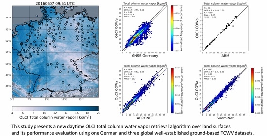
1. Introduction
Atmospheric water vapour plays an important role in both climate and weather. On large spatial and temporal scales, the amount of water vapour has a high impact on Earth’s climate and its evolution through the exchange of energy by latent heat transport, acting as a strong greenhouse gas, and accompanying radiative feedbacks, e.g., [1,2]. Despite extensive research using numerous well-established climate models, large uncertainties exist in the spatio-temporal variability of atmospheric water vapour as well as in the estimates of its radiative forcing and climate sensitivity, e.g., [3,4,5]. To evaluate and improve the model representation of water vapour and its interaction with, e.g., clouds and radiation, comprehensive water vapour observations are needed. Consequently, the Global Climate Observing System (GCOS; https://gcos.wmo.int/, accessed on 1 March 2021) has declared the total column water vapour (TCWV) as a variable critical for characterising the climate system and its changes, i.e., local and global trends.
On smaller temporal and spatial scales, the amount of water vapour in the atmosphere can shape local weather conditions because of its important role in the hydrological cycle. Numerous studies have shown that due to its abundance in the lower tropospheric layers and the coupling with surface processes, it plays a very active role in small-scale boundary layer processes like convective initiation, e.g., [6,7,8]. Still, accurate representations of small-scale water vapour variabilities and related atmospheric processes in numerical weather prediction models are challenging, e.g., [9,10]. In particular the prediction of accompanying high-impact weather phenomena like thunderstorms and heavy precipitation, remains problematic, e.g., [11,12].
To face all these challenges, a wide range of TCWV observational data sets have been developed through the years. In the frame of obtaining an overview and assessing the quality of a number of long-term water vapour data records from satellite-, in-situ and ground-based observations, including reanalyses as well, the Global Energy and Water cycle Exchanges (GEWEX, [13]) Data and Assessments Panel (GDAP) has initiated the GEWEX Water vapour Assessment (G-VAP, [14]) in 2011. Through the analyses and inter-comparisons of the data records, the current state of the art of water vapour products for climate applications is quantified. Please note that in the wider literature different terms are used for TCWV, all representing the same quantity, including for example integrated water vapour (IWV) and total precipitable water (TPW).
Of these existing TCWV observational data sets, only passive imagers on polar-orbiting satellites provide a daily (near) global coverage with high accuracy. Over the oceans, a number of TCWV retrieval methods for measurements from microwave radiometers (MWRs), e.g., the Special Sensor Microwave/Imager (SSM/I), e.g., [15,16] have been established since many years. Over land surfaces, which exhibit stronger heterogeneity, a number of TCWV retrieval methods using measurements in the visible and near-infrared part of the spectrum have been established. Specifically, measurements in the -absorption band, between 890 and 1000 nm, for which all land surfaces types are bright enough, allow the accurate retrieval of TCWV at high spatial resolutions down to several hundred meters [17,18,19,20,21]. The differential absorption technique, using the ratio of measurements in the -absorption band and a nearby window band, is applied by [22] to cloud-free observations of the Medium Resolution Imaging Spectrometer (MERIS) onboard Envisat to create global time series of TCWV [23]. To fill the temporal gap between observations from MERIS and its follow-up instrument Ocean and Land Colour Instrument (OLCI) on-board the Sentinel-3 satellites, the optimal estimation (OE) procedure for MERIS TCWV retrievals [22] was successfully adapted for near-infrared (NIR) measurements of the Moderate Resolution Imaging Spectroradiometer (MODIS) on-board Aqua and Terra satellites [24].
Despite the relatively low temporal sampling of MODIS and MERIS-based TCWV observations, a study on their representativeness shows only a minor impact of the limited time of observation of the morning overpass in comparison to daily means [25]. However, all NIR based TCWV observations require clear sky conditions, which occasionally can lead to a dry bias of up to 5 kg/m2 for TCWV monthly means compared to all sky observations. Using ground-based TCWV measurements from a dense German Global Navigation Satellite System (GNSS) network as reference, it was shown that the temporal, clear-sky and daytime satellite sampling limitations only marginally affect TCWV means, though significant changes can be observed in the TCWV frequency distributions [26]. The potential of the high spatial resolution TCWV observations in the order of hundred meters for the detection and quantification of small-scale structures, related to convective features, was demonstrated for a MERIS case [27].
The launch of the Copernicus Sentinel-3a and Sentinel-3b satellites [28], in the years 2016 and 2018, respectively, and their on-board OLCI instruments, provides for continuity with the Envisat MERIS mission. While the European Space Agency’s (ESAs) primary OLCI mission is the observation of sea and land surfaces, a secondary objective relates to the accurate retrievals and descriptions of the atmospheric state. One part is the operational TCWV retrieval. It is based on the method designed for MERIS [22]. It makes use of the MERIS-heritage bands thus only one of the two water vapour absorption bands. In the framework of the Improvement in Copernicus Sentinel-3 OLCI Water Vapour product (COWa) project (see https://www.eumetsat.int/COWA, accessed on 1 March 2021) an improved TCWV retrieval algorithm for OLCI is set up and first validation studies are performed [29,30]. The aim of COWa is to fully exploit OLCI’s extended spectral capabilities by using the two bands sensitive to water vapour absorption. [31] has shown that this reduces the uncertainty in comparison to a retrieval using only one absorption band. The retrieval method is based on the full OE method, thus providing also TCWV uncertainty estimates on a pixel-bases, in addition it is easily transferable to other NIR-based TCWV observations.
Although we have set up separate forward models for land and water surfaces, the focus in this work is on the presentation and validation of the enhanced OLCI COWa TCWV retrievals for land surfaces only. The Sentinel-3 satellites carry microwave radiometers which allow accurate TCWV estimates over the oceans for the sub-satellite track [32], but the accuracy of the retrievals suffers over land due to very variable and high surface emissivities. This further emphasises the need to obtain accurate TCWV retrievals over land from OLCI observations.
The structure of this paper is as follows. In Section 2, the OLCI instrument, its L1 and L2 data and four well-established observational TCWV reference data sets are introduced. In Section 2.3, the OLCI COWa TCWV retrieval method is described, with details on the forward model, including a new correction for water vapour absorption, and on the inversion technique with accompanying uncertainty estimations. Validation results on a global scale and for the region of Germany (from now on called the German domain) are presented in Section 3. In addition, a first evaluation of the OLCI COWa pixel-based TCWV uncertainty estimates is introduced. Finally, a discussion is given in Section 4.
2. Data and Methodology
In the following, the OLCI instrument technical characteristics and corresponding L1 and L2 data, that serve as input in the COWa TCWV retrieval algorithm, are specified. Furthermore, also four well-established TCWV ground-based observational data sets, based on different measurement and retrieval techniques, are described. They serve as reference data sets in the validation study of the COWa TCWV product, which is presented in Section 3.
2.1. OLCI
The Sentinel-3 OLCI instruments are based on the opto-mechanical and imaging design of ENVISAT MERIS. The instrument is a quasi-autonomous, self-contained, visible pushbroom imaging spectrometer and incorporates the following significant improvements when compared to MERIS:
- An increase in the number of spectral bands from 15 to 21;
- Improved signal-to-noise-ratio (SNR) and a 14-bit analogue to digital converter;
- Improved long-term radiometric stability;
- Mitigation of sun-glint contamination by tilting cameras in westerly direction by 12.6°;
- Complete coverage over both land and ocean at 300 m Full-Resolution (FR);
- Improved instrument characterisation including stray-light, camera overlap, and calibration diffusers;
- Pixel specific spectral characterisation (central wavelength, bandwidth, solar irradiance).
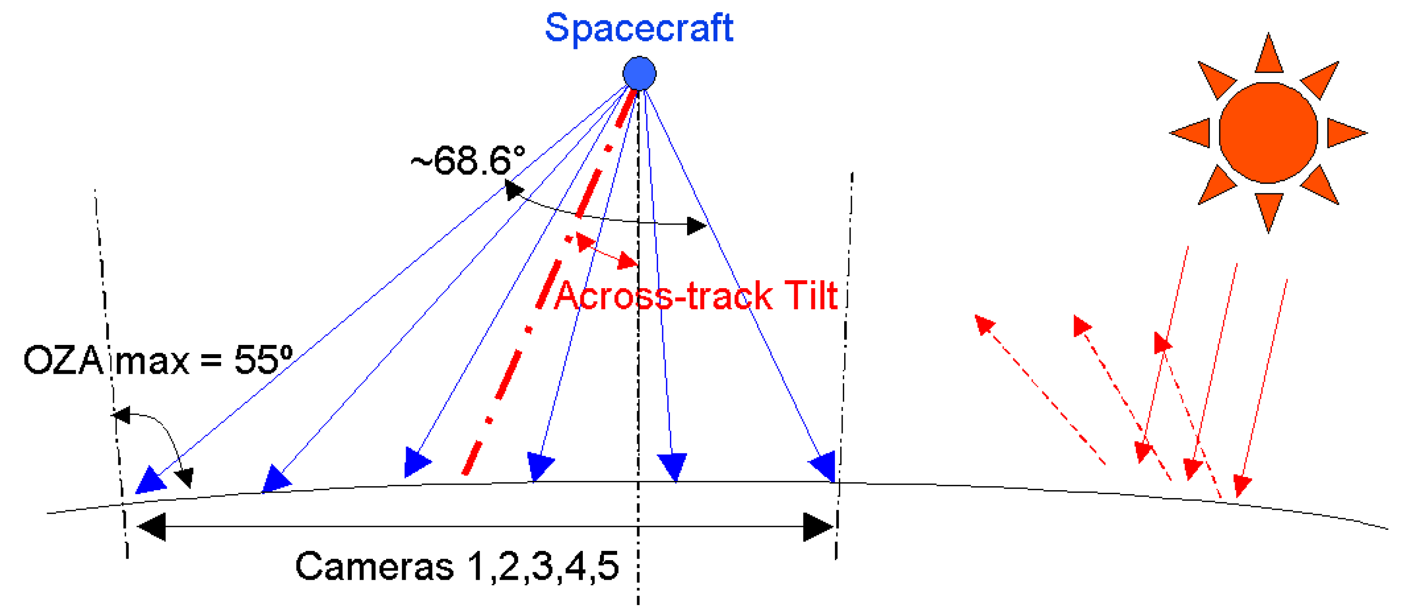
The cameras are arranged to slightly overlap with each other to cover a wide 68.5° across-track field of view. See Figure 1 and Table 1 for further technical details. An additional band Oa21 at 1.02 m, in comparison to MERIS, has been included to improve atmospheric and aerosol correction capabilities, and additional channels in the O2A-band at around 762 nm spectral region are included for improving cloud detection. Furthermore, these channels are also providing information to improve cloud top pressure retrievals. While MERIS had two bands for the retrieval of TCWV, band Me14 as a reference and band Me15 as the water vapour absorption band, OLCI has one additional reference band (Oa21) and one additional water vapour absorption band Oa20, see Table 2.
2.1.1. L1 and L2 Data
The COWa processor is using radiances normalised to the corresponding inband solar irradiance , as defined in Equation (1).
is the extraterrestrial solar irradiance averaged over the relative spectral response of band i. The observation geometry is expressed in viewing zenith angle, sun zenith angle and azimuth difference angle. All used quantities are conveniently provided in the standard L1b product-files including auxiliary data: sea level pressure , surface elevation h, air temperature at surface and eventually total column water vapour from European Centre for Medium-Range Weather Forecasts (ECMWF) analyses, using the Non Time Critical (NTC) OLCI data, for a first guess. The surface pressure is estimated from surface elevation (in m) and sea level pressure by using the international barometric formula:
L2 data are used for cloud masking by applying the standard flags CLOUD, CLOUD AMBIGUOUS and CLOUD MARGIN. This is fully consistent with the standard OLCI L2 water vapour product (see next section).
2.1.2. L2 Standard TCWV Product
OLCI’s standard L2 products for Land (OL_2_LFR/OL_2_LRR) and Water (OL_2_ WFR/OL_2_WRR) contain a total column water vapour field (parameter name IWV) for cloud free pixel. It is based on a differential absorption technique using the combination of the water vapour absorption band Oa19 and the near-by non-absorbing reference bands Oa17 and Oa18. It builds on the heritage of the TCWV retrieval algorithm designed for MERIS measurements [22] (see Table 2). The water vapour column above a pixel is eventually estimated by comparing Radiative Transfer (RT) based simulations with the corresponding OLCI measurements. The RT-simulations are approximated by a product of the atmospheric transmission (using exponential sums of pre-calculated uncorrelated k-distribution terms) and an estimation of the scattering—absorption—interaction, quantified by a factor and stored in a look-up table (LUT). The optimisation with respect to the total column water vapour is done by a one-dimensional gradient descent (Newton secant method) (see also https://sentinel.esa.int/web/sentinel/technical-guides/sentinel-3-olci/level-2/water-vapour-retrieval, accessed on 1 March 2021).
For the cloud detection, the standard L2 cloud-mask has been applied, including the cloud ambiguous and cloud margin flags (see also https://sentinel.esa.int/web/sentinel/technical-guides/sentinel-3-olci/level-2/pixel-classification, accessed on 1 March 2021). For all OLCI L2 products error estimates are provided. The performance of the OLCI standard TCWV product for both Sentinel-3a and Sentinel-3b are presented in several studies, e.g., [33,34].
2.2. Reference TCWV Data Sets
A validation study of the new OLCI COWa and OLCI standard TCWV products is performed for observations over land surfaces only (Section 3). On a global scale, the validation is performed via comparisons with ground-based measurements of water vapour from the Aerosol Robotic Network (AERONET) and Global Navigation Satellite System (GNSS). The comparison against the measurements from microwave radiometer on Atmospheric Radiation Measurement (ARM) sites serves as a consistency check, to be explained in Section 2.3.3. For a German domain, the validation is performed via comparison to observations from the dense German GNSS network. In the following a short description of the ground-based instruments and corresponding TCWV products is given.
2.2.1. ARM
Three fixed and continuously operated, as well as several mobile, multi-platform ARM site facilities are spread globally, covering diverse climate regimes with the aim to provide detailed and accurate description of the Earth’s atmosphere, especially atmospheric radiative processes, with the aim to resolve the uncertainties in climate and earth system models [35]. The two-channel microwave radiometers (MWRs) are designed to measure the downwelling radiation emitted by atmospheric water vapour and liquid water at frequencies of 23.8 GHz and 31.4 GHz [36]. The temporal resolution of the MWRs is 20 s. Since there is only insignificant uncertainty introduced by the background emission of the cold space, ground-based microwave data are considered as one of the most accurate methods for the determination of the water vapour column amount. The measurement uncertainty is expected to be in the range of 0.3 kg/m2 [37].
2.2.2. AERONET
Frequent and long-term measurements of atmospheric parameters, focusing on aerosol optical properties and precipitable water, are provided for hundreds of AERONET sites distributed over the globe [38]. The sun photometer instruments measure the downwelling radiances within the -absorption band, for which just like with OLCI measurements, the TCWV can be retrieved. For this study, global TCWV values from the Direct Sun Algorithm Version 2 [39,40,41] were collected (downloaded from https://aeronet.gsfc.nasa.gov, accessed on 1 March 2021) The temporal resolution depends on the scanning settings of the local sun photometer instrument and varies between 2 and 20 min. In [42], it is stated that the analysed AERONET based TCWV retrievals in-close a consistent dry bias of approximately 5–6% and an estimated uncertainty of 12–15%.
2.2.3. U.S. SuomiNet
GNSS networks provide long-term and accurate TCWV data sets for a large number of locations, including thousands of Global Positioning System (GPS) stations, around the globe and are widely used in research involving water vapour observations. In this study we use the near-global U.S. SuomiNet (UCAR/COSMIC) TCWV product [43], consisting of about 400 GPS stations for the year 2018. This large network provide TCWV values retrieved from consistently processed GPS measurements of the temperature- and humidity-dependent zenith path delay at a couple of hundred sites with a temporal resolution of 30 min. For a detailed description of the analysis method and the data set see [44]. The uncertainty of this TCWV product is not precisely stated by the authors, however similar data sets published accuracies of 1–2 kg/m2 [45,46].
2.2.4. German GNSS Network
In Germany a dense GNSS network provides measurements, with no limitations in respect to weather conditions and time of day, at a temporal resolution of 15 min. The Geoforschungszentrum Potsdam (GFZ) processes data of approximately 300 GPS stations operationally and in near-real time (NRT) using the EPOS software [45]. The estimated travel time of a signal from various GPS satellites to a receiver at the ground-based station, depends on the atmospheric state along the travel such as the water vapour amount. The part of the signal delay attributed to water vapour amount, the so called wet delay, is, in combination with meteorological observations of temperature and pressure at the GPS station, related to TCWV. For this study, the TCWV data set was downloaded from the Standardized Atmospheric Measurement Data (SAMD) Archive [47,48]. The months for the time period May-September 2018 were provided separately by the University of Cologne and processed with the same retrieval framework used for the production of the TCWV data set archived in SAMD. The TCWV is provided with an accuracy of 1–2 kg/m2 [45].
2.3. Retrieval Method
In the following, the principles of the proposed TCWV procedure is sketched, which can be classified as a 1D-Var approach. The forward operator is expressed as look-up tables, which have been calculated by means of radiative transfer simulations taking into account various atmospheric conditions. To be independent of solar cycles, and time of year, normalised radiances are used (see Equation (1)). A 1D-Var scheme optimises the difference between simulated and measured radiances by iteratively varying the TCWV value and additional state parameter, following the scheme after Rodgers [49] (see Section 2.3.5).
2.3.1. Physical Background
Water vapour has various absorption features in the solar and terrestrial spectrum, which is due to a combination of the three fundamental vibration modes, their overtone and rotational transition of the water molecule. Measurements of reflected sunlight in the -absorption band enable a determination of TCWV if the following conditions are given:
- Solar radiation is available, limiting the retrieval to daytime measurements
- The band measuring the absorption is located in a sensitive part of the spectrum but not saturated.
- The surface brightness in the absorption band can be estimated.
- The lower troposphere, holding the main part of the TCWV, is not masked by clouds or optically thick aerosol layers.
For monochromatic radiation, neglecting scattering processes along the photon path, the transmittance T through the atmosphere can be related to its optical depth and the air mass along the geometrical path following the Bouguer-Lambert-Beer law. The optical depth of a medium is a measure of the amount of attenuating species, here the extinction cross section of water vapour molecules multiplied by their number density and integrated along the geometric path. However, the absorption measured by a medium resolution satellite instrument cannot be quantified by the simple Bouguer-Lambert-Beer law, since the band average transmission results from the superposition of many individual absorption lines, whereby their depths and widths result from pressure- and temperature dependent broadening processes. Consequently, the knowledge of the actual temperature-pressure profile is necessary in order to simulate the correct atmospheric transmittance. References [22,50] showed, that it is sufficient to use the surface pressure and the 2 m-temperature to approximate the transmittance corresponding to the actual temperature profile by adequately mixing the pre-calculated transmittance values corresponding to two close standard profiles.
In NIR, the scattering is dominated by mostly forward scattering aerosols and thus the geometrical path coincides well with photon path. Therefore, the effect of single and multiple scattering on aerosols is usually only a few percent of the direct reflected solar radiation in the NIR region, nevertheless it is not negligible as shown and quantified by [22] using a scattering factor f. In particular, above dark surfaces, where a large part of the photons is reflected by atmospheric scatterers and thus does not travel through the whole vertical column of water vapour, the scattering must be precisely considered. However, in the NIR spectral range almost all land surfaces provide a good background (surface albedo > 0.1).
2.3.2. Forward Model
For the forward operator, radiative transfer simulations were performed for various atmospheric conditions and stored in look-up tables. The needed gaseous absorption coefficients, based on HITRAN 2016 data [51], were calculated using an advanced k-distribution routine for different standard temperature profiles [20,52]. Eventually, the used absorption optical thicknesses were modified as described in [24] and in Section 2.3.3. Interactions with aerosol particles and molecules are simulated with the radiative transfer Matrix Operator Model (MOMO) [53]. Over land, the surface is assumed to be Lambertian. The standard forward operator is an n-dimensional linear interpolation in the pre-calculated LUTs, having the state vector elements and auxiliary data as dimensions, see Table 3. However, the forward model is exchangeable; a full online radiative transfer simulator like Radiative Transfer for TOVS (RTTOV; [54]) or different LUT parameterisations can be used. Depending on the surface type, the algorithm uses different sets of state parameters and additional parameters assumed to be fixed. Over land, the retrieved state consists of the surface albedo in the window bands and the TCWV. The surface temperature and pressure constrain the choice of the assumed temperature profile. The aerosol optical thickness constrains the atmospheric state further. The priors for the atmospheric state are taken from ECMWF analysis (non-time critical) or forecast (for near-realtime analysis).
The forward operator used in the TCWV retrieval is a generic module that provides simulated radiances measured by a satellite under specific atmospheric conditions. The subset of all physical parameters relevant for the radiative transfer that is retrieved, is here called the state vector. The remaining parameters are fully constrained (not variable) during the retrieval, in particular the
- Aerosol type (continental or maritime aerosol);
- Aerosol scale height (1500 m);
- Profile of temperature and humidity;
- Aerosol optical depth (above land only, from climatology);
- Central wavelength of the absorption bands (see Section 3.3).
2.3.3. Correction of Simulated Water Vapour Absorption
Reference [24] found a systematic overestimation of TCWV from MODIS NIR measurements compared to ground based microwave radiometer measurements. They identified several possible reasons: (i) deficits in spectral and radiometric characterisation of the MODIS bands, (ii) deficits in NIR forward simulations and (iii) a systematic underestimation of the microwave radiometer-based retrievals. The latter was excluded, since the wet bias was consistently found when compared to ground based GPS measurement and radiosonde observations. They further excluded spectral calibration reasons by analysing synthetic sensitivity tests. These findings are consistent with TCWV retrievals from OLCI. First, there is a systematic overestimation of about 10 percent (see Section 3.1). Second, OLCI’s standard TCWV retrieval does not show distinct camera-dependent features, although the central wavelength of the bands jump by more than 1.2 nm between some of the 5 cameras. The origin of the deficiency of the retrieval is not known yet. It could lay in the description of water vapour absorption, in particular in the insufficient description of the continuum absorption or broadening effects. However, instrument effects (e.g., over or under-corrected spectral stray light) cannot be ruled out either. Hence, they introduced correction coefficients in order to adjust the atmospheric transmittance. We follow this approach.
is the optical thickness of water vapour absorption, is the corrected optical thickness. The coefficients a and b were obtained by minimising the difference between the simulated and measured OLCI observations using the ARM-MWR data set as a reference (see Section 2.2.1). It is important to note, that this was done for the bands 19 and 20 individually. The derived correction coefficients are given in Table 4.
2.3.4. OLCI-A/B Camera Dependent Spectral Shifts
Due to the optical design of OLCI’s five cameras, all spectral bands show a slightly varying spectral response over the field of view, and further small discontinuities at the four transitions between the cameras. The first moment of the relative spectral response, the central wavelength, exhibits variations of up to 1 nm within one camera and jumps of up to 1.6 nm between the cameras [55]. Retrievals using spectral channels within or close to varying absorption bands are sensitive to these spectral shifts, which must be considered in associated retrieval processes, such as for the MERIS O2A-band cloud top pressure retrieval [56]. Previous retrievals of spectral shifts on MERIS and OLCI water vapour retrievals have indicated that the shifts and jumps are small enough to be neglected [22], but this was simply based on the non-visibility of discontinuities of the water vapour fields on the camera boundaries.
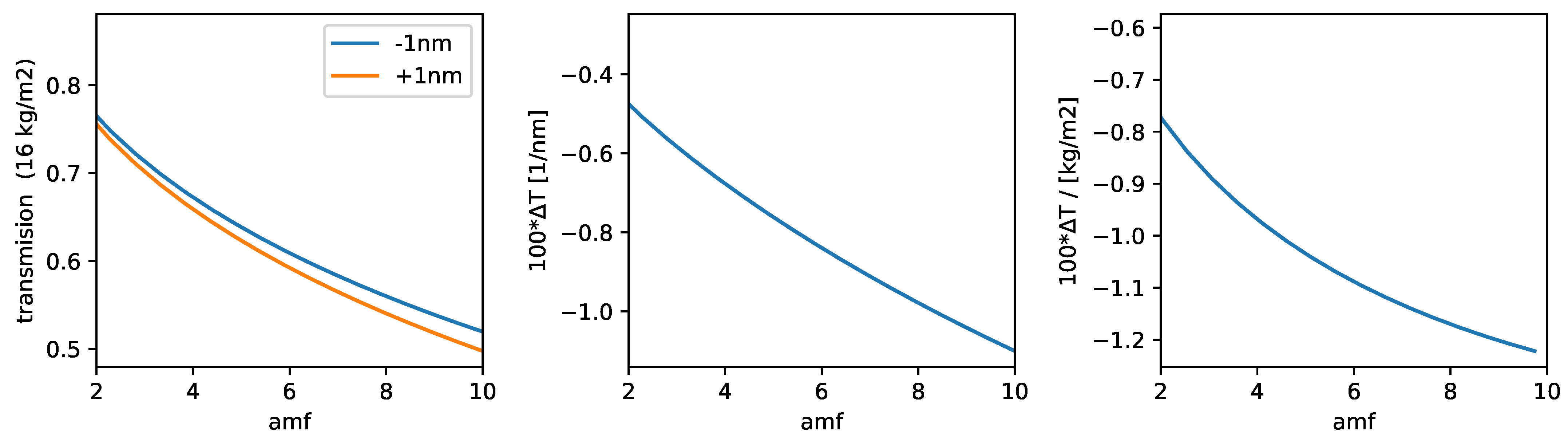
A first investigation quantifies the impact of a spectral-shift of 1 nm on the atmospheric transmission of band Oa19 for a U.S. Standard Atmosphere [57] with a total water vapour column of 16 kg/m2. The transmission changes between 0.005 and 0.011 (depending on the air mass factor), when the central wavelength is shifted from 901 nm to 899 nm. Increasing the water vapour by 1 kg/m2 changes the transmission in the same order magnitude (see Figure 2). For this specific case 1nm uncertainty of the spectral location of the band corresponds to approximately 0.5 kg/m2 (3%) uncertainty of the retrieved water vapour column. Comparing to, e.g., the root mean squared difference between OLCI’s and SuomiNets TCWV, which is in the order of 10%, it follows that uncertainty of the spectral characterisation of OLCI contributes significantly to the uncertainty of retrieved water vapour column (see Section 3).
2.3.5. Inversion Technique
This retrieval estimates TCWV values with the help of an inverse modelling scheme. Deviations between modelled and measured radiances as well as between the estimated state and the prior knowledge about the state are iteratively reduced, using a variational method. The uncertainties are estimated by taking into account all known uncertainty influences.
The estimation of a state vector X based on a measurement Y and a priori knowledge is considered as optimal, if the following cost function is minimised:
With and being the measurement and a priori error co-variance matrices, respectively, and a forward model calculating a measurement from a state X.
This approach assumes Gaussian probability density functions and bias-free measurements, priors and models. There are several methods to find the optimal solution of Equation (4). If the dependencies between state vector X and measurement Y are not high-frequency (ideally the cost is convex) or if a first guess estimation in the convex vicinity of the optimal solution exists (thus a solver does not trap into local minima), gradient-based methods can be used, such as: Steepest Descent, Gauss–Newton, Levenberg–Marquardt and Newton method. The commonality among them is, that starting from a first guess they iteratively approximate the optimal solution using gradient (the Jacobian) or (approximations of) the second order derivatives (the Hessian) for the update step .
The OLCI COWa TCWV retrieval algorithm is using the Gauss–Newton update step:
The iteration is stopped when the maximum number of iterations is reached or when the following criterion is met (see Rodgers [49]):
n is the number parameter in the state vector and is adjustable, e.g., to 0.01. , the retrieval error co-variance is detailed further in Section 2.3.6. The first guess of TCWV is taken from model predictions or analysis.
A common and useful treatment of an inverse problem to increase convergence speed is to transform it to a ‘more linear’ form. We transformed the measurement in the absorption bands to quantities , which almost linearly depend on the total amount of water vapour by:
where is the top of atmosphere reflectance in bands 19 or 20, AMF is the air mass factor, is top of atmosphere reflectance of the window bands () inter- or extrapolated to the wavelength of the absorption band:
With that in mind, is a kind of rectified optical thickness, which is roughly proportional to the amount of water vapour, the only absorbing atmospheric constituent around 0.9 m.
2.3.6. Uncertainty Estimates
Uncertainty estimates are provided by considering all relevant sources of error such as sensor noise, and errors of forward modelling parameters such as aerosol optical thickness, aerosol vertical distribution, wind speed, surface elevation and temperature. Eventually, the algorithm relies on a strict prior cloud detection. Undetected clouds can lead to underestimation of TCWV, due to shielding effects as well as to overestimation of TCWV due to multiple scattering effects.
To incorporate forward model uncertainties is composed from the error co-variance matrix of the measurement (from, e.g., instrument signal noise ratio at signal level) and from the forward model parameter error co-variance . is the Jacobian of the forward model F with respect to its parameterisations B:
The retrieval uncertainty is part of the update step (see Equation (6)):
considering the following sources of uncertainty:
- Measurement uncertainty (SNR)
- Uncertainty of the aerosol optical depth (assumed to be 0.1)
- Uncertainty of the surface pressure and temperature (assumed to be 5 K and 5 hPa).
Since the measurement is transformed, the corresponding measurement error co-variance must be transformed too. Assuming that the SNR is approximately the same for all bands and a simple uncertainty propagation of Equations (8) and (9), the uncertainty in the transformed absorption bands is:
Here we assume an uncertainty (of 0.01) due to the extra- or interpolation of the window bands to the absorption bands.
3. Results
3.1. Validation on Global Scale
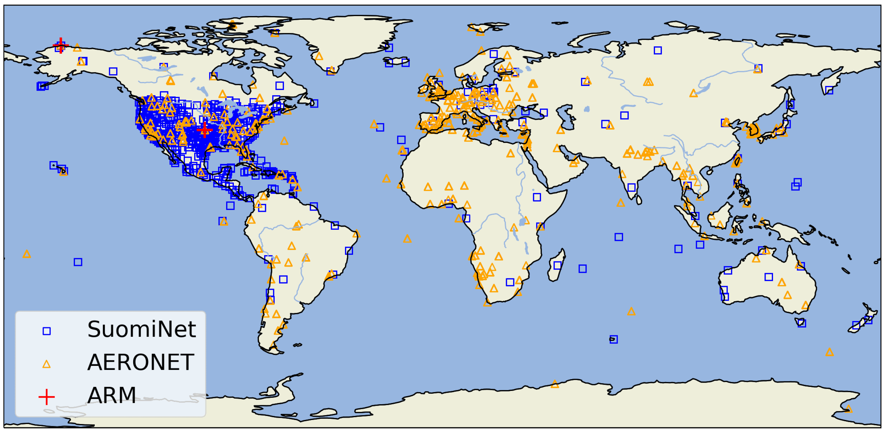
Match-ups between OLCI COWa TCWV data set, as well as the standard OLCI L2 TCWV data set, and the three reference TCWV data sets from globally distributed ground-based measurement sites, see Figure 3, have been created for the period of November 2017 to October 2018. For the validation, cloud-free and valid pixels, i.e., with a cost < 1 (Equation (4)), above land were averaged within an area around each ground station within the ARM, AERONET and SuomiNet data sets. For the cloud detection, the OLCI standard L2 cloud-mask has been applied, including the cloud ambiguous and cloud margin flags. To include a match-up in the validation exercise the 3 × 3 OLCI pixel area centred around the ground-based station needs to be 100% cloud free, while at least 90% of the pixels within the surrounding averaging area needs to be cloud free. To minimise disturbing effects such as undetected cloud, inaccurate geo-location and different observing geometries, an averaging of the reference TCWV measurements within a 15 min time frame around the Sentinel-3 OLCI overpass has been performed.
3.1.1. ARM
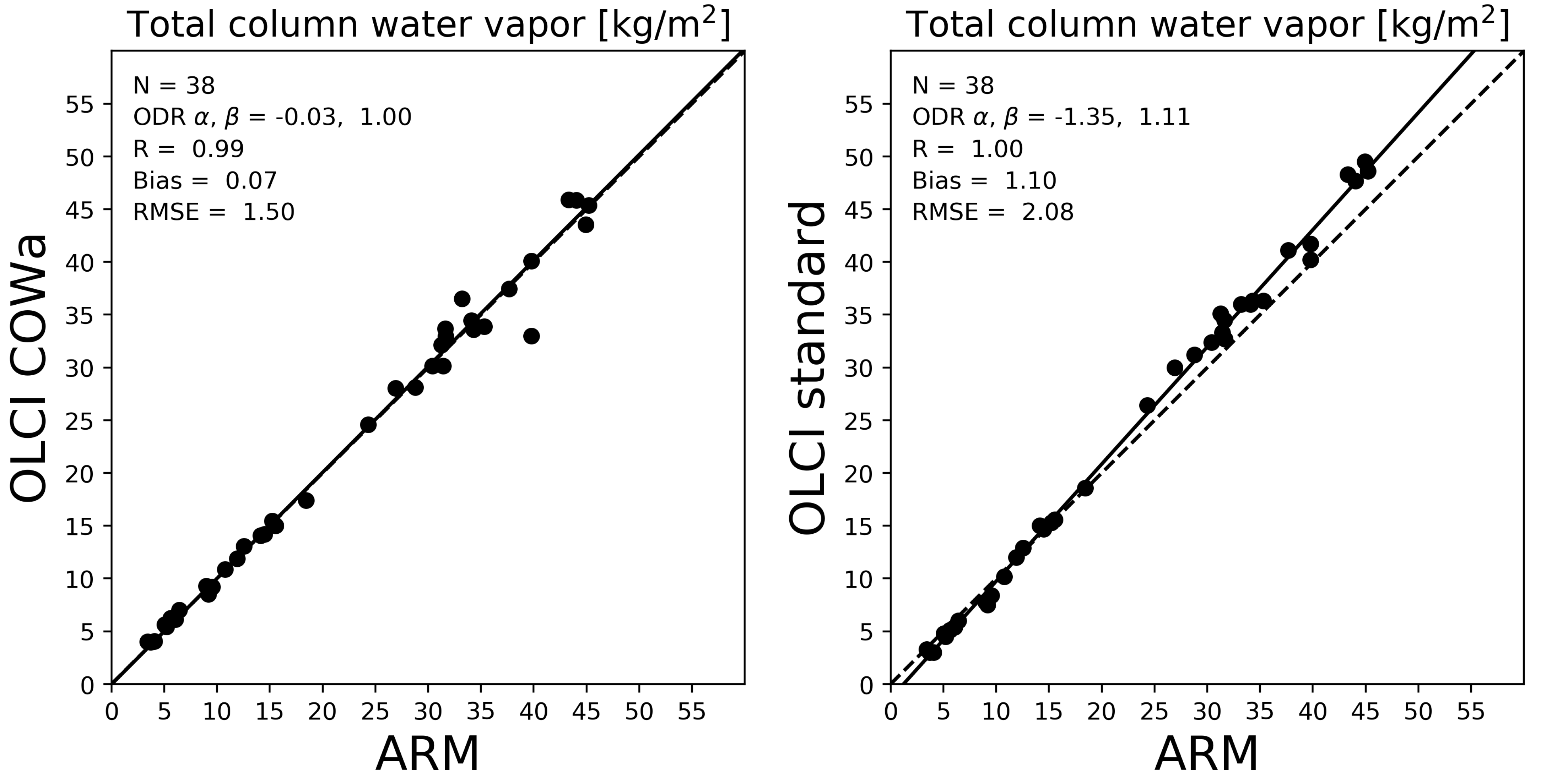
Currently three ARM sites are operated continuously, two of them over land, see Figure 3, resulting in a limited number of suitable MWR-OLCI collocated measurements. For the comparison, valid OLCI TCWV pixels were averaged within a 10 × 10 km area around each ARM site. As described in Section 2.3.3, the ARM TCWV product was used to introduce correction coefficients for atmospheric transmittance calibration, and thus the comparison serves as a consistency check.
The comparison of the OLCI COWa TCWV retrievals against the ARM TCWV retrievals for the 38 match-ups show a high agreement, see Figure 4 (left panel). The correlation between both quantities is 0.99 for the OLCI COWa TCWV product and even 1.00 for the OLCI standard TCWV product. However, both the OLCI COWa root mean square error (RMSE) and bias, 0.07 kg/m2 and 1.10 kg/m2, respectively, are significantly smaller than for the standard OLCI TCWV product, see Figure 4 (right panel). While the standard OLCI TCWV product shows a systematic overestimation of 11%, using orthogonal distance regression (ODR) [58,59], which takes the uncertainties of both products into account, the OLCI COWa TCWV product does not show any wet-bias.
3.1.2. AERONET
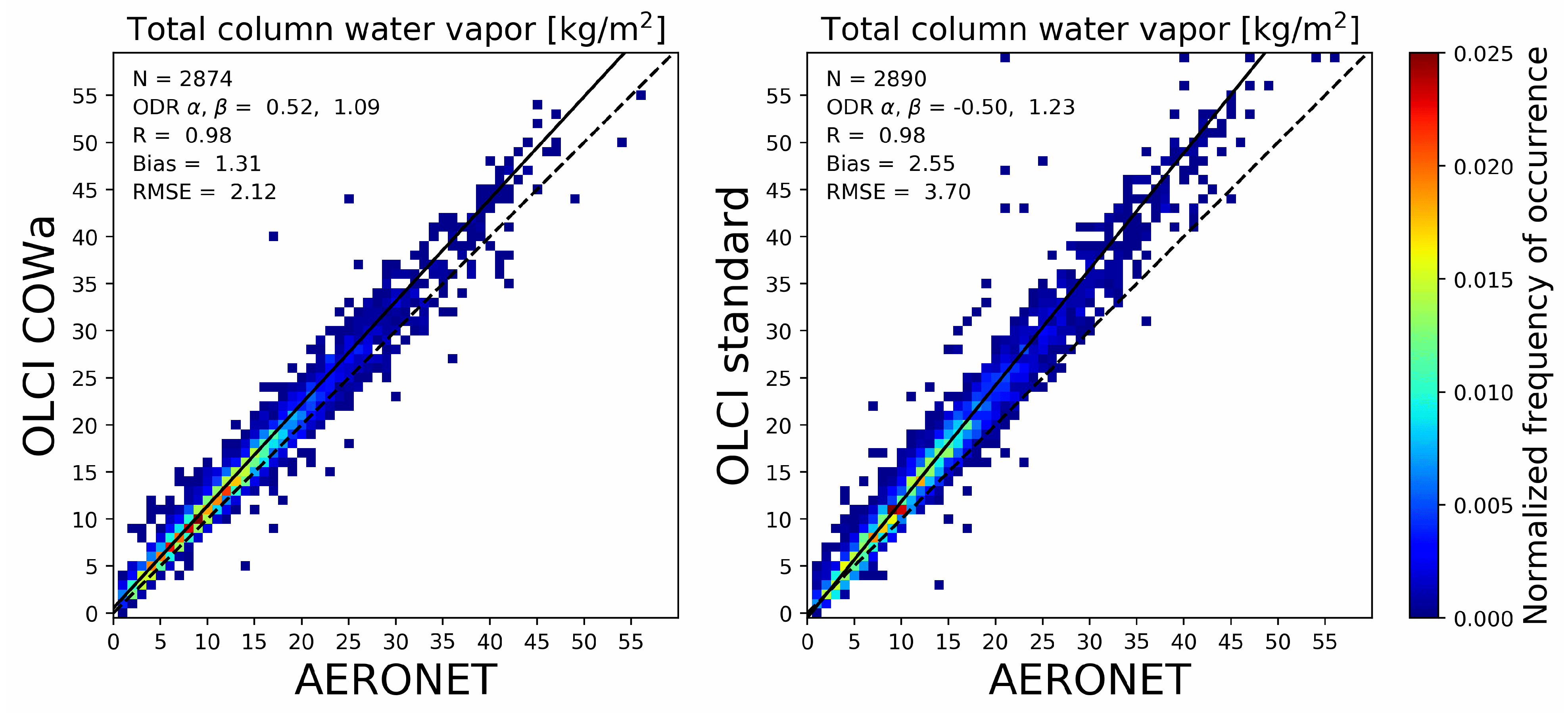
The AERONET sites are distributed over the globe, though the largest concentration of sites can be found in Europe, see Figure 3. For the comparison, valid OLCI TCWV pixels were averaged within a 10 km × 10 km area around each AERONET site.
The comparison of the OLCI COWa TCWV retrievals against the AERONET TCWV retrievals for nearly 3000 match-ups show a good agreement, see Figure 5 (left panel). The correlation between both quantities is 0.98. Both the RMSE and bias, 2.21 kg/m2 and 1.31 kg/m2, respectively, are significantly smaller than for the standard OLCI TCWV product, see Figure 5 (right panel). The COWa TCWV products shows a significant smaller wet-bias of 9%, using ODR, compared to the wet-bias of 23% for the standard OLCI TCWV product.
3.1.3. SuomiNet
The U.S. SuomiNet sites are distributed over the globe, covering both low and high elevations, however, the majority of these GPS stations are located in North-America and Central-America, see Figure 3. For the comparison, valid OLCI TCWV pixels were averaged within an 10 km × 10 km area around each GPS station.
The comparison of the OLCI COWa TCWV retrievals against the SuomiNet TCWV retrievals for nearly 3000 match-ups show a very good agreement, see Figure 6 (left panel). The correlation between both quantities is 0.99 for both OLCI TCWV products. Both the RMSE and bias, 0.42 kg/m2 and 1.19 kg/m2, respectively, are significantly smaller than for the standard OLCI TCWV product, see Figure 6 (right panel). The COWa TCWV products shows a nearly zero smaller wet-bias of 2%, using ODR, while the standard OLCI TCWV product shows a wet-bias of 14%.
3.2. Validation in German Domain
A match-up data set between the OLCI COWa TCWV product and the TCWV product from a dense German GNSS network has been created for the spring and summer months April to September for the years 2016 to 2018. Winter and autumn months were left out to reduce the uncertainty in the assessment due to problematic OLCI TCWV retrievals related to large solar zenith angles and misclassified snow surfaces. The cloud-free and valid OLCI pixels, i.e., cost < 1., closest to the location of each GPS station are taken. Further constraints include 100% cloud free conditions for the 3 × 3 OLCI pixels centred around the GPS station and 90% cloud free conditions in the surrounding area within an area with a radius of 15 km. Furthermore, the maximum allowed difference between the height of the GPS station and the mean height within the OLCI pixel was set to 100 m. For this, the free Digital Elevation Model (DEM) from NASA’s Shuttle Radar Topography Mission (SRTM) [60] with a spatial resolution of 83 m was used. The maximum time difference between the OLCI observations and the GPS observations is 7.5 min.
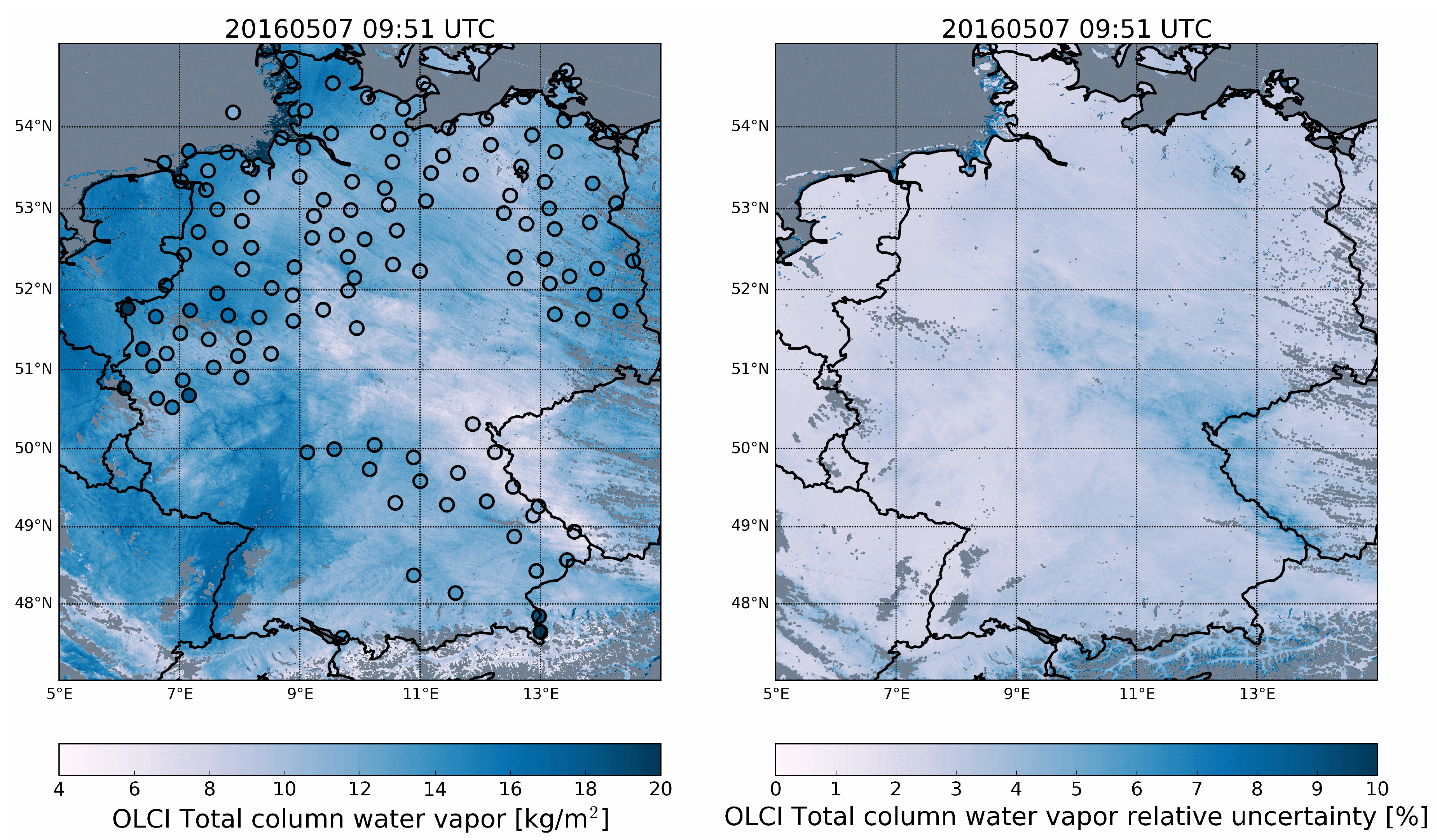
In Figure 7, an example of retrieved TCWV values and corresponding uncertainties for an OLCI overpass in the German domain for a mostly clear-sky morning in May 2016 is shown, including the locations of the GPS station for which valid match-ups could be created that day. The TCWV field shows large-scale variabilities, with TCWV values ranging from about 6 kg/m2 in the south-east to about 20 kg/m2 in the northwest. Corresponding TCWV relative uncertainties range from about 2 to 4% for the higher TCWV values, while they can go up to 7–9% for the lower TCWV values. Note that this example also shows TCWV retrievals over water surfaces, for which the corresponding uncertainties are much higher. This is expected since the dark water surface leads to low signal return. However, those retrievals are not further analysed in this study. Furthermore, small-scale variabilities, e.g., in the form of alternating lines of high and low TCWV values, most clearly visible in the northern part of the domain, can be observed. In the eastern part cloud streets have developed, indicated by the grey pixels, which extent further in the domain later in the morning (not shown). Without in-depth analysis of this specific case, still parallels can be found with the MERIS observations of horizontal convective rolls described in [26].
The comparison of the OLCI COWa TCWV retrievals against the GNSS TCWV retrievals for more than 4000 match-ups show a small dry bias of 0.34 kg/m2 and a relatively large RMSE of 3.26 kg/m2, see Figure 8. Similar findings were done in [26] for the comparison of the MODIS-FUB TCWV retrieval against GNSS TCWV for the year 2013, with a small dry bias of −0.31 kg/m2 and a RMSE of 2.52 kg/m2. Furthermore, here, a bi-modal distribution can be observed, with the two maxima located around higher values of 13 and 17 kg/m2, attributed to the daytime and clear-sky sampling [26]. The correlation between both quantities is 0.89. Using ODR, a wet-bias of 11% is found.
3.3. A First Evaluation of Pixel-Based TCWV Uncertainty Estimates
An evaluation framework as described in [61] is used to assess the quality of the TCWV uncertainty estimates provided by the optimal estimation retrieval scheme. It is based on expected statistical properties of ensembles of estimated uncertainties and observed retrieval errors. In this study, the OLCI COWa TCWV uncertainty estimates are evaluated using the global match-up AERONET TCWV data set and corresponding uncertainties (described in Section 2.2.2) as a reference. Out of the three reference TCWV data sets used in this study, the AERONET data set provides the best global and seasonal coverage, including a large variety of environmental and meteorological conditions. Another advantage is the use of an inherent cloud masking method [62] and not having a fixed, but a relative uncertainty estimate, while the GPS-based data sets do not provide an uncertainty estimate per measurement.
The total expected discrepancy, , between OLCI COWa TCWV and AERONET TCWV for one single match-up takes into account the uncertainties of both TCWV retrievals, and , respectively, assuming they are independent of one another. Since the TCWV match-ups are not perfect in space and time, also the spatial and temporal variability are taken into account. Here, the spatial variability is represented by the standard deviation, , computed from the OLCI pixel-based TCWV retrievals in an area around the AERONET station. The temporal variability is represented by the standard deviation, , computed from the AERONET TCWV retrievals within 15 min of the OLCI overpass time. Thus, the total expected discrepancy is given by,
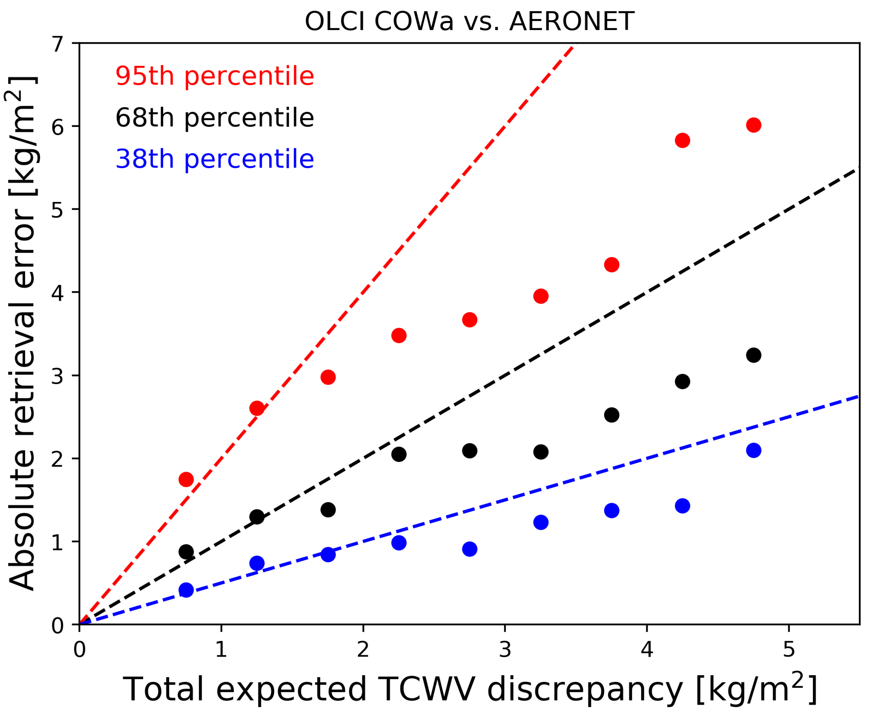
The total expected discrepancy, i.e., estimated uncertainty, is compared to the actual retrieval errors, i.e., , to assess consistency with the expectations, see Figure 9. The is stratified into bins of 0.5 kg/m2 and for each bin a quantile analysis is performed in terms of computation of the 38th, 68th and 95th percentile. Assuming Gaussian distributions, these percentiles relate to 0.5, 1 and 2 standard deviations, respectively. Random selection of match-ups was done such that each bin is equally populated.
In general, the total expected TCWV discrepancy increases with absolute retrieval error. Up to about 1.5–2 kg/m2 expected discrepancy the uncertainty estimates are very close to theoretical expectations. This is especially relevant for the 68th percentile, which directly relates to the expectation of the retrieval error of 1 standard deviation. For larger discrepancies there is an overall tendency for the uncertainty estimates to be too large.
Nonetheless, it is shown that despite the fact that the magnitude of the estimated uncertainties are overestimated for higher retrieval errors, from about 3 kg/m2 on wards, the distributions of the retrieval errors within each discrepancy bin are roughly Gaussian.
4. Discussion
This work presents a newly developed daytime TCWV retrieval for OLCI-A and -B measurements over cloud-free land surfaces. It builds on retrieval methods developed for the precursor passive imager MERIS [22] as well as for MODIS [24], but significant extensions have been applied, taking advantage of the improved observing capabilities of OLCI.
During the development of the algorithm, we found systematic deviations between OLCI measurements and simulations. The microwave measurements at the ARM site in the southern great plains Oklahoma, where the atmospheric condition could precisely be determined, could be used to reduced the systematic bias. Unconsidered, the deviations would lead to a wet bias. A wet bias has also been found in the current operational retrieval and for former MERIS and MODIS algorithms. The systematic bias could be compensated by a simple linear correction of the atmospheric transmittance, which likewise has also been applied for MERIS and MODIS [24]. We are currently investigating, if the modification of the absorption optical thickness is consistent with ground based observations of direct solar irradiance measurements. For this, the time series of the Precision Solar Spectroradiometer (PSR; [63]) and Pandora [64,65,66] measurements at the Lindenberg observatory in Germany, are used. If the absorption correction is not necessary for the ground observations, it would be reasonable to assume satellite instrument specificities.
The presented COWa algorithm is fully capable of being used with observations from instruments similar to OLCI, like the previous MERIS and MODIS. Basically, the used look-up tables have to be exchanged and the instrument specific systematic deviations have to be quantified and corrected, if necessary (see Section 2.3.3). Within ESA’s water vapour climate change initiative (CCI; https://climate.esa.int/en/projects/water-vapour, accessed on 1 March 2021) this path is currently committed in order to create climate data records of TCWV. A first evaluation showed a high agreement of the respective datasets, however small systematic discrepancies ≤ 1 kg/m2 have been found and are subject of investigations.
The validation study is performed using four well-established ground-based TCWV observation data sets on a global scale as well as for a German domain. For the comparison, valid OLCI TCWV pixels were averaged within a 10 km × 10 km area around each ground-based observation site. We acknowledge that this window is somewhat arbitrary. However, considering that we need to take into account aspects such as different geometry views and advection processes, this size allows in Reduced Resolution (RR) Mode (10 km 9 pixel) the safe calculation of distribution parameters, like mean, median and standard deviation. We are not aware of a matchup-protocol, like it is for example used in the Ocean Color research community, which we could follow. We experimented with sizes of, e.g., 5 × 5 or 3 × 3 pixels in RR mode, which gave virtually the same results for the mean, and slightly different results for the root mean squared difference between ground truth and satellite-based TCWV observations. Hence, we included the spatial variability in the estimation of the total expected discrepancy, which is needed for the evaluation of the retrieval uncertainty (see Section 3.3). The comparison against the ARM TCWV product, which serves as a consistency check, shows a bias and RMSE of 0.07 kg/m2 and 1.10 kg/m2. This near-zero bias for OLCI COWa indicates that the inclusion of the atmospheric transmittance correction coefficients in the TCWV retrieval framework was successful. The comparisons against the AERONET and U.S. SuomiNet TCWV products show biases of 1.31 kg/m2 and 0.42 kg/m2, and RMSEs of 2.12 kg/m2 and 1.35 kg/m2, respectively. For the comparison against the TCWV products from the German GNSS sites, a bias and RMSE of −0.34 kg/m2 and 3.26 kg/m2, respectively, was found. This compares well, despite a somewhat larger RMSE, with earlier findings for the MODIS TCWV retrievals [26] based on [24]. In the comparisons to all global reference data sets the estimated OLCI standard TCWV product, which shows significantly larger systematic overestimations and RMSEs, and the OLCI COWa TCWV products shows the superior performance of the latter.
The results from a first evaluation study of OLCI COWa TCWV uncertainties, using AERONET TCWV dataset as reference, show an overestimation of expected TCWV discrepancy for larger retrieval errors, which is computed from the absolute difference between the observed TCWV from AERONET and OLCI COWa. For absolute retieval errors below about 3 kg/m2, the expected TCWV discrepancy is close to the theoretical expectations. This could mean that the OLCI COWa retrieval error budget is too pessimistic and possibly related to forward model errors which are not properly accounted for within the OLCI COWa optimal estimation retrieval framework. Alternatively, it could mean that the AERONET uncertainties are overestimated. We tend to lean to the latter, since a relative uncertainty estimate of 12 to 15%, especially for larger TCWV values, seems very high. This would also explain the larger overestimation of estimated uncertainty at the high end, i.e., 95th percentile, of each binned distribution. Similar overestimation of estimated uncertainty was found for higher discrepancies when not including the spatial and temporal variability in the total expected discrepancy (not shown).
It has to be emphasised that the overall performance of the TCWV retrieval algorithm strongly depends on the reliability of the cloud mask. Since OLCI does not provide measurements in the thermal infrared, the screening of clouds is difficult. A dry bias is to be expected where the cloud detection fails.
5. Conclusions
The OLCI COWa TCWV retrieval method is based on a differential absorption technique, making use of measurements in the -absorption band and near-by window bands, and can be easily adapted for different sensors which measure reflected sunlight in this spectral region. The 1D-Var algorithm is based on a fast forward model, in the form of high dimensional linear look up table interpolation. Uncertainties are provided on a pixel-basis, based on uncertainties of measurements (SNRs) and the forward model assumptions. The improvements with respect to the precursor TCWV retrieval methods designed for MERIS, which the current operational OLCI standard TCWV retrieval algorithm is based on, and MODIS relate to the:
- exploitation of the extended spectral capabilities;
- improvement in the inversion scheme by introducing a complete optimal estimation scheme including linear error characterisation;
- set-up designed for flexible forward operator use and application to similar types of observations, certainly from OLCI on future Sentinel-3 satellites, but also, e.g., from future Flexible Combined Imager (FCI) on Meteosat Third Generation (MTG; [67]) and METimage on Metop - Second Generation (Metop-SG; [68]).
TCWV measurements at an ARM site over the Southern Great plains were used to apply a correction for atmospheric transmittance in order to overcome systematic biases that were also found in earlier studies. A comparison to the ARM TCWV product showed a near-zero bias and RMSE of 0.07 kg/m2 and 1.10 kg/m2. Using three other well-established ground-based TCWV datasets for validation on both a global scale for the years 2017–2018 and for a region in Germany for the months April-September for the years 2016–2018 showed biases and RMSEs ranging from −0.34 kg/m and 2.12 kg/m and 0.42 kg/m and 3.26 kg/m, respectively. These validation results, performed for TCWV retrievals from OLCI-A measurements, show that the proposed algorithm has acceptable accuracy. A first evaluation of uncertainties is performed using the AERONET TCWV product and accompanying uncertainty estimates as reference. A total expected TCWV discrepancy is computed from a squared sum of both OLCI COWa and AERONET TCWV uncertainties and the spatial and temporal variabilities related to each observational match-up. Despite the overall tendency of the uncertainty estimates to be too large relative to the observed retrieval error, the distribution of the retrieval errors is roughly Gaussian for the observed TCWV discrepancies.
In future validation studies, the inclusion of additional ground-based and radiosonde reference TCWV datasets like the GCOS Reference Upper-Air Network (GRUAN; https://www.gruan.org, accessed on 1 March 2021) and radiosonde observations (RaOBs) are under consideration, for which time delays between the observations need to be accounted for. Moreover, TCWV retrievals from OLCI-B will be included, which will increase sampling size and the corresponding match-up dataset significantly.
Several improvements of the OLCI COWa TCWV retrieval algorithm are envisaged for the near future. First, a complete account of the varying central wavelength over OLCI’s field of view will be included in the forward model. This is to appreciate, that the deviation of the real spectral characteristics from the assumed nominal values is responsible for a small but significant part to the uncertainty budget (see Section 2.3.4). For a next OLCI L1 reprocessing the inclusion of radiance uncertainties on a pixel by pixel basis is envisaged. These uncertainties will then be propagated in the optimal estimation framework. Furthermore, a forward model for water surfaces is under development. Here, also information on wind speeds and aerosol optical depth are taken into account. For conditions, where the sun glint provides sufficient surface reflectance, water vapour columns can be retrieved. Low reflectance conditions in off-glint regions will still be improper, because the observation of the full atmospheric column is inhibited. Additional information could be gathered from co-located thermal infrared measurements with moderate water vapour influences, like the 3.7, 11 and 12 µm bands of Sea and Land Surface Temperature Radiometer (SLSTR; [69]).
The new OLCI COWa TCWV product is already subject of assimilation studies. First analysis of the OLCI/Sentinel-3a TCWV land product against the UK-met-office assimilation product shows that OLCI can improve the atmospheric state for numerical weather prediction with respect to water vapour (Rodger Saunders, pers. Com. 2020). What is more, the potential of using OLCI’s high spatial resolution TCWV observations for convective initiation detection, i.e., observing small-scale convective structures in a TCWV field before the onset of clouds and precipitation, is investigated within the German project Near-Realtime Quantitative Precipitation Estimation and Prediction (RealPEP; https://www2.meteo.uni-bonn.de/realpep/, accessed on 1 March 2021).
Author Contributions
Conceptualization, R.P., C.C.H., J.F.; methodology, R.P., C.C.H.; software, R.P., C.C.H.; validation, R.P., C.C.H.; formal analysis, R.P., C.C.H.; investigation, R.P., C.C.H.; resources, R.P., J.F., C.C.H.; data curation, R.P., C.C.H.; writing—original draft preparation, C.C.H., R.P.; writing—review and editing, C.C.H. and R.P.; visualization, C.C.H., R.P.; supervision, J.F. All authors have read and agreed to the published version of the manuscript.
Funding
The research was funded by the Deutsche Forschungsgemeinschaft (DFG, German Research Foundation) - FOR 2589 (RealPEP), by EUMESTSAT-Contract: EUM/CO/16/4600002115/EJK and by ESA-Contract: /400012355418/I-NB.
Data Availability Statement
Publicly available datasets were analyzed in this study. The data can be found here: ftp://jericho.met.fu-berlin.de/pub/data_remotesensing-13-00932 accessed on 1 March 2021.
Acknowledgments
We would like to thank Susanne Crewell and Christopher Frank from the University of Cologne for providing the GNSS data set for Germany for the year 2018. We thank all researchers and staff for establishing and maintaining the AERONET sites used in this investigation. Furthermore, we acknowledge the ground-based observational networks ARM, SuomiNet and GNSS, as well as the SAMD archive, for providing TCWV products. The publication of this article was funded by Freie Universität Berlin.
Conflicts of Interest
The authors declare no conflict of interest.
Abbreviations
The following abbreviations are used in this manuscript:
| 1D-Var | 1-Dimensional Variational |
| AERONET | Aerosol Robotic Network |
| ARM | Atmospheric Radiation Measurement |
| COWa | Improvement in Copernicus Sentinel-3 OLCI Water Vapour Product |
| ECMWF | European Centre for Medium-Range Weather Forecasts |
| EUMETSAT | European Organisation for the Exploitation of Meteorological Satellites |
| FUB | Freie Universität Berlin |
| GCOS | Global Climate Observing System |
| GNSS | Global Navigation Satellite Systems |
| GPS | Global Positioning System |
| L1/L2 | Level 1/Level 2 |
| LBL | Line-by-line |
| LUT | Look-up Table |
| MERIS | Medium Resolution Imaging Spectrometer Instrument |
| MOMO | Matrix Operator Model |
| MODIS | Moderate Resolution Imaging Spectroradiometer |
| MSG/MTG | Meteosat Second/Third Generation |
| MWR | Microwave Radiometer |
| NIR | Near Infrared |
| ODR | Orthogonal Distance Regression |
| OE | Optimal Estimation |
| OLCI | Ocean and Land Colour Instrument |
| RMSE | Root Mean Square Error |
| RTTOV | Radiative Transfer for TOVS (TIROS Operational Vertical Sounder) |
| SEVIRI | Spinning Enhanced Visible and Infrared Imager |
| SNR | Signal-to-noise-ratio |
| STD | Standard Deviation |
| TCWV | Total Column Water Vapour |
References
- Bengtsson, L. The global atmospheric water cycle. Environ. Res. Lett. 2010, 5, 025202. [Google Scholar] [CrossRef]
- Stevens, B.; Bony, S. Water in the atmosphere. Phys. Today 2013, 66, 29–34. [Google Scholar] [CrossRef] [Green Version]
- Held, I.M.; Soden, B.J. Water vapor feedback and global warming. Annu. Rev. Energy Environ. 2000, 25, 441–475. [Google Scholar] [CrossRef] [Green Version]
- Lacis, A.A.; Schmidt, G.A.; Rind, D.; Ruedy, R.A. Atmospheric CO2: Principal control knob governing Earth’s temperature. Science 2010, 330, 356–359. [Google Scholar] [CrossRef] [PubMed] [Green Version]
- Hegerl, G.C.; Black, E.; Allan, R.P.; Ingram, W.J.; Polson, D.; Trenberth, K.E.; Chadwick, R.S.; Arkin, P.A.; Sarojini, B.B.; Becker, A.; et al. Challenges in quantifying changes in the global water cycle. Bull. Am. Meteorol. Soc. 2019, 100, 1097–1115. [Google Scholar] [CrossRef] [Green Version]
- Weckwerth, T.M.; Parsons, D.B. A review of convection initiation and motivation for IHOP_2002. Mon. Weather Rev. 2006, 134, 5–22. [Google Scholar] [CrossRef]
- Keil, C.; Röpnack, A.; Craig, G.C.; Schumann, U. Sensitivity of quantitative precipitation forecast to height dependent changes in humidity. Geophys. Res. Lett. 2008, 35. [Google Scholar] [CrossRef] [Green Version]
- Sherwood, S.; Roca, R.; Weckwerth, T.; Andronova, N. Tropospheric water vapor, convection, and climate. Rev. Geophys. 2010, 48. [Google Scholar] [CrossRef] [Green Version]
- Dierer, S.; Arpagaus, M.; Seifert, A.; Avgoustoglou, E.; Dumitrache, R.; Grazzini, F.; Mercogliano, P.; Milelli, M.; Starosta, K. Deficiencies in quantitative precipitation forecasts: Sensitivity studies using the COSMO model. Meteorol. Z. 2009, 18, 631–645. [Google Scholar] [CrossRef]
- Naumann, A.K.; Kiemle, C. The vertical structure and spatial variability of lower-tropospheric water vapor and clouds in the trades. Atmos. Chem. Phys. 2020, 20, 6129–6145. [Google Scholar] [CrossRef]
- Bauer, H.S.; Schwitalla, T.; Wulfmeyer, V.; Bakhshaii, A.; Ehret, U.; Neuper, M.; Caumont, O. Quantitative precipitation estimation based on high-resolution numerical weather prediction and data assimilation with WRF–a performance test. Tellus A Dyn. Meteorol. Oceanogr. 2015, 67, 25047. [Google Scholar] [CrossRef]
- Mugume, I.; Basalirwa, C.; Waiswa, D.; Nsabagwa, M.; Ngailo, T.J.; Reuder, J.; Semujju, M. A Comparative Analysis of the Performance of COSMO and WRF Models in Quantitative Rainfall Prediction. Int. J. Mar. Environ. Sci. 2018, 12, 130–138. [Google Scholar]
- Chahine, M.T. GEWEX: The global energy and water cycle experiment. Eos Trans. Am. Geophys. Union 1992, 73, 9–14. [Google Scholar] [CrossRef]
- Schröder, M.; Lockhoff, M.; Shi, L.; August, T.; Bennartz, R.; Borbas, E.; Brogniez, H.; Calbet, X.; Crewell, S.; Eikenberg, S.; et al. GEWEX water vapor assessment (G-VAP). World Climate Research Programme (WCRP) Publication; WMO: Geneva, Switzerland, 2017. [Google Scholar]
- Schluessel, P.; Emery, W.J. Atmospheric water vapour over oceans from SSM/I measurements. Int. J. Remote Sens. 1990, 11, 753–766. [Google Scholar] [CrossRef]
- Wentz, F.J. A well-calibrated ocean algorithm for special sensor microwave/imager. J. Geophys. Res. Ocean. 1997, 102, 8703–8718. [Google Scholar] [CrossRef] [Green Version]
- Fischer, J. High Resolution Spectroscopy for Remote Sensing of Physical Cloud Properties and Water Vapour; Deepak Publishing: Hampton, VR, USA, 1988. [Google Scholar]
- Gao, B.C.; Goetz, A.F. Column atmospheric water vapor and vegetation liquid water retrievals from airborne imaging spectrometer data. J. Geophys. Res. Atmos. 1990, 95, 3549–3564. [Google Scholar] [CrossRef]
- Bartsch, B.; Bakan, S.; Fischer, J. Passive remote sensing of the atmospheric water vapour content above land surfaces. Adv. Space Res. 1996, 18, 25–28. [Google Scholar] [CrossRef]
- Bennartz, R.; Fischer, J. A modified k-distribution approach applied to narrow band water vapour and oxygen absorption estimates in the near infrared. J. Quant. Spectrosc. Radiat. Transf. 2000, 66, 539–553. [Google Scholar] [CrossRef]
- Albert, P.; Bennartz, R.; Preusker, R.; Leinweber, R.; Fischer, J. Remote sensing of atmospheric water vapor using the moderate resolution imaging spectroradiometer. J. Atmos. Ocean. Technol. 2005, 22, 309–314. [Google Scholar] [CrossRef]
- Lindstrot, R.; Preusker, R.; Diedrich, H.; Doppler, L.; Bennartz, R.; Fischer, J. 1D-Var retrieval of daytime total columnar water vapour from MERIS measurements. Atmos. Meas. Tech. 2012, 5, 631. [Google Scholar] [CrossRef] [Green Version]
- Lindstrot, R.; Stengel, M.; Schröder, M.; Fischer, J.; Preusker, R.; Schneider, N.; Steenbergen, T.; Bojkov, B. A global climatology of total columnar water vapour from SSM/I and MERIS. Earth Syst. Sci. Data 2014, 6, 221–233. [Google Scholar] [CrossRef] [Green Version]
- Diedrich, H.; Preusker, R.; Lindstrot, R.; Fischer, J. Retrieval of daytime total columnar water vapour from MODIS measurements over land surfaces. Atmos. Meas. Tech. 2015, 8, 823–836. [Google Scholar] [CrossRef] [Green Version]
- Diedrich, H.; Wittchen, F.; Preusker, R.; Fischer, J. Representativeness of total column water vapour retrievals from instruments on polar orbiting satellites. Atmos. Chem. Phys. 2016, 16, 8331–8339. [Google Scholar] [CrossRef] [Green Version]
- Carbajal Henken, C.; Dirks, L.; Steinke, S.; Diedrich, H.; August, T.; Crewell, S. Assessment of Sampling Effects on Various Satellite-Derived Integrated Water Vapor Datasets Using GPS Measurements in Germany as Reference. Remote Sens. 2020, 12, 1170. [Google Scholar] [CrossRef] [Green Version]
- Carbajal Henken, C.; Diedrich, H.; Preusker, R.; Fischer, J. MERIS full-resolution total column water vapor: Observing horizontal convective rolls. Geophys. Res. Lett. 2015, 42. [Google Scholar] [CrossRef]
- Donlon, C.; Berruti, B.; Buongiorno, A.; Ferreira, M.H.; Féménias, P.; Frerick, J.; Goryl, P.; Klein, U.; Laur, H.; Mavrocordatos, C.; et al. The global monitoring for environment and security (GMES) sentinel-3 mission. Remote Sens. Environ. 2012, 120, 37–57. [Google Scholar] [CrossRef]
- Preusker, R.; Fischer, J. Algorithm Theoretical Basis Document—Improvement in Copernicus Sentinel-3 OLCI Water Vapour Product—COWa; Technical Report; EUMETSAT: Dramstadt, Germany, 2020. [Google Scholar]
- Preusker, R.; Fischer, J. Algorithm Product Validation and Evolution Report—Improvement in Copernicus Sentinel-3 OLCI Water Vapour Product—COWa; Technical report; EUMETSAT: Dramstadt, Germany, 2020. [Google Scholar]
- Diedrich, H.; Preusker, R.; Lindstrot, R.; Fischer, J. Quantification of uncertainties of water vapour column retrievals using future instruments. Atmos. Meas. Tech. 2013, 6, 359–370. [Google Scholar] [CrossRef]
- Frery, M.L.; Siméon, M.; Goldstein, C.; Féménias, P.; Borde, F.; Houpert, A.; Olea Garcia, A. Sentinel-3 Microwave Radiometers: Instrument Description, Calibration and Geophysical Products Performances. Remote Sens. 2020, 12, 2590. [Google Scholar] [CrossRef]
- Mertikas, S.; Partsinevelos, P.; Tripolitsiotis, A.; Kokolakis, C.; Petrakis, G.; Frantzis, X. Validation of Sentinel-3 OLCI Integrated Water Vapor Products Using Regional GNSS Measurements in Crete, Greece. Remote Sens. 2020, 12, 2606. [Google Scholar] [CrossRef]
- Sentinel-3 OLCI Report. Available online: https://sentinels.copernicus.eu/documents/247904/4069162/Sentinel-3-MPC-ACR-OLCI-Cyclic-Report-056-037.pdf (accessed on 1 March 2021).
- Stokes, G.M.; Schwartz, S.E. The Atmospheric Radiation Measurement (ARM) Program: Programmatic background and design of the cloud and radiation test bed. Bull. Am. Meteorol. Soc. 1994, 75, 1201–1222. [Google Scholar] [CrossRef]
- Turner, D.D.; Clough, S.A.; Liljegren, J.C.; Clothiaux, E.E.; Cady-Pereira, K.E.; Gaustad, K.L. Retrieving Liquid Wat0er Path and Precipitable Water Vapor From the Atmospheric Radiation Measurement (ARM) Microwave Radiometers. IEEE Trans. Geosci. Remote Sens. 2007, 45, 3680–3690. [Google Scholar] [CrossRef]
- Turner, D.D.; Lesht, B.M.; Clough, S.A.; Liljegren, J.C.; Revercomb, H.E.; Tobin, D. Dry bias and variability in Vaisala RS80-H radiosondes: The ARM experience. J. Atmos. Ocean. Technol. 2003, 20, 117–132. [Google Scholar] [CrossRef] [Green Version]
- Holben, B.N.; Eck, T.F.; Slutsker, I.A.; Tanre, D.; Buis, J.; Setzer, A.; Vermote, E.; Reagan, J.A.; Kaufman, Y.; Nakajima, T.; et al. AERONET—A federated instrument network and data archive for aerosol characterization. Remote Sens. Environ. 1998, 66, 1–16. [Google Scholar] [CrossRef]
- Bruegge, C.J.; Conel, J.E.; Green, R.O.; Margolis, J.S.; Holm, R.G.; Toon, G. Water vapor column abundance retrievals during FIFE. J. Geophys. Res. Atmos. 1992, 97, 18759–18768. [Google Scholar] [CrossRef]
- FoxTx, R. A simple instrument and technique for measuring columnar water vapor via near-IR differential solar transmission measurements. IEEE Trans. Geosci. Remote Sens. 1992, 30, 825–831. [Google Scholar]
- Holben, B.N.; Eck, T.; Slutsker, I.; Smirnov, A.; Sinyuk, A.; Schafer, J.; Giles, D.; Dubovik, O. AERONET’s version 2.0 quality assurance criteria. In Remote Sensing of the Atmosphere and Clouds; International Society for Optics and Photonics: Bellingham, WA, USA, 2006; Volume 6408, p. 64080Q. [Google Scholar]
- Pérez-Ramírez, D.; Whiteman, D.N.; Smirnov, A.; Lyamani, H.; Holben, B.N.; Pinker, R.; Andrade, M.; Alados-Arboledas, L. Evaluation of AERONET precipitable water vapor versus microwave radiometry, GPS, and radiosondes at ARM sites. J. Geophys. Res. Atmos. 2014, 119, 9596–9613. [Google Scholar] [CrossRef] [Green Version]
- Ware, R.H.; Fulker, D.W.; Stein, S.A.; Anderson, D.N.; Avery, S.K.; Clark, R.D.; Droegemeier, K.K.; Kuettner, J.P.; Minster, J.B.; Sorooshian, S. SuomiNet: A real-time national GPS network for atmospheric research and education. Bull. Am. Meteorol. Soc. 2000, 81, 677–694. [Google Scholar] [CrossRef] [Green Version]
- Wang, J.; Zhang, L.; Dai, A.; Van Hove, T.; Van Baelen, J. A near-global, 2-hourly data set of atmospheric precipitable water from ground-based GPS measurements. J. Geophys. Res. Atmos. 2007, 112. [Google Scholar] [CrossRef] [Green Version]
- Gendt, G.; Dick, G.; Reigber, C.; Tomassini, M.; LIU, Y.; Ramatschi, M. Near real time GPS water vapor monitoring for numerical weather prediction in Germany. J. Meteorol. Soc. Jap. Ser. II 2004, 82, 361–370. [Google Scholar] [CrossRef] [Green Version]
- Ge, M.; Gendt, G.; Dick, G.; Zhang, F.; Rothacher, M. A new data processing strategy for huge GNSS global networks. J. Geod. 2006, 80, 199–203. [Google Scholar] [CrossRef]
- Lammert, A.; Hansen, A.; Ament, F.; Crewell, S.; Dick, G.; Grützun, V.; Klein-Baltink, H.; Lehmann, V.; Macke, A.; Pospichal, B.; et al. A Standardized Atmospheric Measurement Data archive for distributed cloud and precipitation process-oriented observations in central Europe. Bull. Am. Meteorol. Soc. 2019, 100, 1299–1314. [Google Scholar] [CrossRef] [Green Version]
- Standardized Atmospheric Measurement Data. Available online: http://doi.org/10.17616/R3D944 (accessed on 1 March 2021).
- Rodgers, C.D. Inverse Methods for Atmospheric Sounding: Theory and Practice; World Scientific: Singapore, 2000; Volume 2. [Google Scholar]
- Lindstrot, R.; Preusker, R. On the efficient treatment of temperature profiles for the estimation of atmospheric transmittance under scattering conditions. Atmos. Meas. Tech. 2012, 5, 2525. [Google Scholar] [CrossRef] [Green Version]
- Rothman, L.S.; Gordon, I.E.; Babikov, Y.; Barbe, A.; Benner, D.C.; Bernath, P.F.; Birk, M.; Bizzocchi, L.; Boudon, V.; Brown, L.R.; et al. The HITRAN2012 molecular spectroscopic database. J. Quant. Spectrosc. Radiat. Transf. 2013, 130, 4–50. [Google Scholar] [CrossRef] [Green Version]
- Doppler, L.; Carbajal-Henken, C.; Pelon, J.; Ravetta, F.; Fischer, J. Extension of radiative transfer code MOMO, matrix-operator model to the thermal infrared–Clear air validation by comparison to RTTOV and application to CALIPSO-IIR. J. Quant. Spectrosc. Radiat. Transf. 2014, 144, 49–67. [Google Scholar] [CrossRef]
- Hollstein, A.; Fischer, J. Radiative transfer solutions for coupled atmosphere ocean systems using the matrix operator technique. J. Quant. Spectrosc. Radiat. Transf. 2012, 113, 536–548. [Google Scholar] [CrossRef]
- Saunders, R.; Hocking, J.; Turner, E.; Rayer, P.; Rundle, D.; Brunel, P.; Vidot, J.; Roquet, P.; Matricardi, M.; Geer, A.; et al. An update on the RTTOV fast radiative transfer model (currently at version 12). Geosci. Model Dev. 2018, 11. [Google Scholar] [CrossRef] [Green Version]
- Sentinel 3 CalVal Team. Technical Note: Sentinel-3 OLCI-A Spectral Response Functions; Reference: S3-TN-ESA-OL-660; Technical Report; ESA: Paris, France, 2016. [Google Scholar]
- Lindstrot, R.; Preusker, R.; Fischer, J. Empirical correction of stray light within the MERIS oxygen A-band channel. J. Atmos. Ocean. Technol. 2010, 27, 1185–1194. [Google Scholar] [CrossRef]
- National Oceanic and Atmospheric Administration and United States. Air Force. In US Standard Atmosphere, 1976; National Oceanic and Atmospheric Administration: Washington, DC, USA, 1976; Volume 76. [Google Scholar]
- Trent, T.; Schröder, M.; Remedios, J. GEWEX water vapor assessment: Validation of AIRS tropospheric humidity profiles with characterized radiosonde soundings. J. Geophys. Res. Atmos. 2019, 124, 886–906. [Google Scholar] [CrossRef] [Green Version]
- Boggs, P.T.; Rogers, J.E. Orthogonal distance regression. Contemp. Math. 1990, 112, 183–194. [Google Scholar]
- Farr, T.G.; Kobrick, M. Shuttle Radar Topography Mission produces a wealth of data. Eos Trans. Am. Geophys. Union 2000, 81, 583–585. [Google Scholar] [CrossRef]
- Sayer, A.M.; Govaerts, Y.; Kolmonen, P.; Lipponen, A.; Luffarelli, M.; Mielonen, T.; Patadia, F.; Popp, T.; Povey, A.C.; Stebel, K.; et al. A review and framework for the evaluation of pixel-level uncertainty estimates in satellite aerosol remote sensing. Atmos. Meas. Tech. 2020, 13, 373–404. [Google Scholar] [CrossRef] [Green Version]
- Smirnov, A.; Holben, B.; Eck, T.; Dubovik, O.; Slutsker, I. Cloud-Screening and Quality Control Algorithms for the AERONET Database. Remote Sens. Environ. 2000, 73, 337–349. [Google Scholar] [CrossRef]
- Gröbner, J.; Kouremeti, N. The Precision Solar Spectroradiometer (PSR) for direct solar irradiance measurements. Sol. Energy 2019, 185, 199–210. [Google Scholar] [CrossRef]
- Cede, A.; Herman, J.; Richter, A.; Krotkov, N.; Burrows, J. Measurements of nitrogen dioxide total column amounts using a Brewer double spectrophotometer in direct Sun mode. J. Geophys. Res. Atmos. 2006, 111. [Google Scholar] [CrossRef] [Green Version]
- Herman, J.; Cede, A.; Spinei, E.; Mount, G.; Tzortziou, M.; Abuhassan, N. NO2 column amounts from ground-based Pandora and MFDOAS spectrometers using the direct-Sun DOAS technique: Intercomparisons and application to OMI validation. J. Geophys. Res. Atmos. 2009, 114. [Google Scholar] [CrossRef] [Green Version]
- Herman, J.; Evans, R.; Cede, A.; Abuhassan, N.; Petropavlovskikh, I.; McConville, G. Comparison of ozone retrievals from the Pandora spectrometer system and Dobson spectrophotometer in Boulder, Colorado. Atmos. Meas. Tech. Discuss. 2015, 8, 3407–3418. [Google Scholar] [CrossRef] [Green Version]
- Ouaknine, J.; Viard, T.; Napierala, B.; Foerster, U.; Fray, S.; Hallibert, P.; Durand, Y.; Imperiali, S.; Pelouas, P.; Rodolfo, J.; et al. The FCI on board MTG: Optical design and performances. International Conference on Space Optics—ICSO 2014; International Society for Optics and Photonics: Cardiff, UK, 2017; Volume 10563, p. 1056323. [Google Scholar]
- Spezzi, L.; Borde, R.; Phillips, P.; Schlüssel, P.; Watts, P. Validation activities for the level 2 geophysical products of the EUMETSAT Polar System-Second Generation (EPS-SG) visible/infrared imager (METimage). In Remote Sensing of Clouds and the Atmosphere XXIII; International Society for Optics and Photonics: Cardiff, UK, 2018; Volume 10786, p. 1078603. [Google Scholar]
- Coppo, P.; Ricciarelli, B.; Brandani, F.; Delderfield, J.; Ferlet, M.; Mutlow, C.; Munro, G.; Nightingale, T.; Smith, D.; Bianchi, S.; et al. SLSTR: A high accuracy dual scan temperature radiometer for sea and land surface monitoring from space. J. Mod. Opt. 2010, 57, 1815–1830. [Google Scholar] [CrossRef]
Figure 1.
OLCI’s tilted field of view with 5 cameras. From https://sentinel.esa.int/web/sentinel/user-guides/sentinel-3-olci (accessed on 1 March 2021).
Figure 1.
OLCI’s tilted field of view with 5 cameras. From https://sentinel.esa.int/web/sentinel/user-guides/sentinel-3-olci (accessed on 1 March 2021).

Figure 2.
Left: Simulated transmission for band Oa19 of a U.S. Standard Atmosphere with a TCWV of 16 kg/m2, spectrally shifted by ±1 nm for different air mass factors (AMF). Middle: Change of the transmission, if band is shifted by 1 nm. Right: Change of the transmission, if TCWV is increased by 1 kg/m2.

Figure 3.
Geographic distribution of ground-based observational sites for the three global validation data sets.
Figure 3.
Geographic distribution of ground-based observational sites for the three global validation data sets.

Figure 4.
Comparison of the OLCI COWa TCWV retrieval algorithm (left) and the OLCI standard TCWV processor (right) against ARM. N is the number of match-ups, ODR and are the orthogonal distance regression coefficients for the intersect and slope, respectively, R is the correlation, RMSE is the root mean square error. The dotted line presents the 1:1 line, the solid black line presents the result of the ODR fit.

Figure 5.
Normalised frequency of occurrence of the TCWV products for the comparison of the OLCI COWa TCWV retrieval algorithm (left) and the OLCI standard TCWV processor (right) against AERONET. Symbols and abbreviations same as in Figure 4.
Figure 5.
Normalised frequency of occurrence of the TCWV products for the comparison of the OLCI COWa TCWV retrieval algorithm (left) and the OLCI standard TCWV processor (right) against AERONET. Symbols and abbreviations same as in Figure 4.

Figure 6.
Normalised frequency of occurrence of the TCWV products for the comparison of the OLCI COWa TCWV retrieval algorithm (left) and the OLCI standard TCWV processor (right) against SuomiNet. Symbols and abbreviations same as in Figure 4.
Figure 6.
Normalised frequency of occurrence of the TCWV products for the comparison of the OLCI COWa TCWV retrieval algorithm (left) and the OLCI standard TCWV processor (right) against SuomiNet. Symbols and abbreviations same as in Figure 4.

Figure 7.
Example of retrieved OLCI TCWV (left) and accompanying uncertainty (right) for the Sentinel-3a overpass over the German domain on 7 May 2016 at around 09.51 UTC. The circles and colours within show the GPS stations with and GNSS TCWV retrievals at the OLCI overpass time for GPS stations with valid retrievals. The gray colour indicates areas for which no retrievals were performed, mostly due to the presence of clouds.

Figure 8.
Normalised frequency of occurrence of the TCWV products for the comparison of the OLCI COWa TCWV retrieval algorithm on a pixel-bases against GNSS Germany. Symbols and abbreviations same as in Figure 4.
Figure 8.
Normalised frequency of occurrence of the TCWV products for the comparison of the OLCI COWa TCWV retrieval algorithm on a pixel-bases against GNSS Germany. Symbols and abbreviations same as in Figure 4.

Figure 9.
Total expected TCWV discrepancy vs. percentiles of absolute retrieval error, , for binned results. The dashed lines show theoretical values for the 38th, 68th and 95th percentile, which in case of Gaussian distribution relate to the 0.5, 1 and 2 standard deviations, respectively.
Figure 9.
Total expected TCWV discrepancy vs. percentiles of absolute retrieval error, , for binned results. The dashed lines show theoretical values for the 38th, 68th and 95th percentile, which in case of Gaussian distribution relate to the 0.5, 1 and 2 standard deviations, respectively.


Table 1.
Technical specification of the OLCI instrument onboard Sentinel-3. Adapted from https://sentinel.esa.int/web/sentinel/user-guides/sentinel-3-olci (accessed on 1 March 2021).
Table 1.
Technical specification of the OLCI instrument onboard Sentinel-3. Adapted from https://sentinel.esa.int/web/sentinel/user-guides/sentinel-3-olci (accessed on 1 March 2021).
| Swath width | 1270 km |
| Field of view | 68.5° |
| Local solar time (LST) | 09:00–10:30 |
| Full resolution (FR) sub-satellite point | 300 m |
| Reduced resolution (RR) sub-satellite point | 1200 m |
| Radiometric accuracy | 2% abs, 0.1% rel |
Table 2.
OLCI bands used in the COWa TCWV retrieval. * Not used in presented retrieval algorithm, but planned to be included in future versions. The MERIS heritage bands are indicated in blue. Adapted from https://sentinel.esa.int/web/sentinel/user-guides/sentinel-3-olci (accessed on 1 March 2021) and [28].
| Band | Centre (nm) | Width (nm) | Function |
|---|---|---|---|
| Oa17 | 865 | 20 | Atmospheric and aerosol correction, clouds, pixel co-registration |
| Oa18 | 885 | 10 | Water vapour absorption reference band/vegetation monitoring |
| Oa19 | 900 | 10 | Water vapour absorption/vegetation monitoring |
| Oa20 | 940 | 20 | Water vapour absorption, Atmospheric correction/aerosol correction |
| Oa21 * | 1015 | 40 | Atmospheric and aerosol correction |
Table 3.
Retrieved physical parameters and forward operator settings, i.e., LUT, for the land retrieval scheme. TCWV = Total Column Water vapour; AL0 and AL1 = Surface albedo in window band 0 and 1; WVC = Water vapour Content; AOT = Aeorsol Optical Depth at 900 nm; PRS = Surface Pressure; TMP = Air Temperature at 2 m; SUZ = Sun Zenith Angle; VIE = Viewing Zenith Angle; AZI = Azimuth difference angle. Note, that the surface pressure and the water vapour column are non-linearly, scaled and transformed with natural logarithm and square root, respectively, in order to increase the linearity.
| Forward Operator | State Vector Parameters | LUT Dimensions and Values |
|---|---|---|
| Land | TCWV AL0 and AL1 | WVC in kg/m2 [0.1, 0.5, 5, 20, 40, 75] AL0 and AL1 [0.001, 0.01, 0.1, 0.3, 1] AOT [0, 0.05, 0.1, 0.2, 0.7] PRS in hPa [1030, 780, 530] TMP in K [263.13, 288.13, 313.13] SUZ and VIE in degree [0, 0.8, 18.9, 28.0, 37.1, 46.1, 55.2, 64.3, 73.4] AZI in degree [0, 18, 36, 54, 72, 90, 108, 126, 144, 162, 180] |
Table 4.
Correction coefficients (see Equation (3)) for the adjustment of the absorption optical thickness of water vapour for OLCI bands 19 and 20.
Table 4.
Correction coefficients (see Equation (3)) for the adjustment of the absorption optical thickness of water vapour for OLCI bands 19 and 20.
| Band | a | b |
|---|---|---|
| 19 | −0.0054 | 1.061 |
| 20 | 0.023 | 1.147 |
Publisher’s Note: MDPI stays neutral with regard to jurisdictional claims in published maps and institutional affiliations. |
© 2021 by the authors. Licensee MDPI, Basel, Switzerland. This article is an open access article distributed under the terms and conditions of the Creative Commons Attribution (CC BY) license (http://creativecommons.org/licenses/by/4.0/).
Share and Cite
MDPI and ACS Style
Preusker, R.; Carbajal Henken, C.; Fischer, J. Retrieval of Daytime Total Column Water Vapour from OLCI Measurements over Land Surfaces. Remote Sens. 2021, 13, 932. https://doi.org/10.3390/rs13050932
AMA Style
Preusker R, Carbajal Henken C, Fischer J. Retrieval of Daytime Total Column Water Vapour from OLCI Measurements over Land Surfaces. Remote Sensing. 2021; 13(5):932. https://doi.org/10.3390/rs13050932
Chicago/Turabian StylePreusker, René, Cintia Carbajal Henken, and Jürgen Fischer. 2021. "Retrieval of Daytime Total Column Water Vapour from OLCI Measurements over Land Surfaces" Remote Sensing 13, no. 5: 932. https://doi.org/10.3390/rs13050932
Note that from the first issue of 2016, this journal uses article numbers instead of page numbers. See further details here.