A Workflow Based on SNAP–StaMPS Open-Source Tools and GNSS Data for PSI-Based Ground Deformation Using Dual-Orbit Sentinel-1 Data: Accuracy Assessment with Error Propagation Analysis

Abstract

This paper discusses a full interferometry processing chain based on dual-orbit Sentinel-1A and Sentinel-1B (S1) synthetic aperture radar data and a combination of open-source routines from the Sentinel Application Platform (SNAP), Stanford Method for Persistent Scatterers (StaMPS), and additional routines introduced by the authors. These are used to provide vertical and East-West horizontal velocity maps over a study area in the south-western sector of the Po Plain (Italy) where land subsidence is recognized. The processing of long time series of displacements from a cluster of continuous global navigation satellite system stations is used to provide a global reference frame for line-of-sight–projected velocities and to validate velocity maps after the decomposition analysis. We thus introduce the main theoretical aspects related to error propagation analysis for the proposed methodology and provide the level of uncertainty of the validation analysis at relevant points. The combined SNAP–StaMPS workflow is shown to be a reliable tool for S1 data processing. Based on the validation procedure, the workflow allows decomposed velocity maps to be obtained with an accuracy of 2 mm/yr with expected uncertainty levels lower than 2 mm/yr. Slant-oriented and decomposed velocity maps provide new insights into the ground deformation phenomena that affect the study area arising from a combination of natural and anthropogenic sources.

1. Introduction

Satellite radar interferometry is recognized as an effective technique in different applications focused on deformation phenomena that occur on the Earth surface. The successful application of this methodology is strictly related to the ability to depict the displacement of ground targets at a very high level of accuracy (1–2 mm/yr) using synthetic aperture radar (SAR) images and time series analysis of displacements oriented along the Line Of Sight (LOS) directions. Since the first applications in the early 1990s, with the first generation of SAR satellites (ERS-1 and Radarsat-1), the temporal and spatial resolution increased, and a number of research fields have taken advantage of satellite radar interferometry. Among these, applications to natural hazard assessment, ground deformation, and investigations into polar cap dynamics, slope failures, and instability processes are relevant to the present study [1,2,3,4,5,6,7].

Differential SAR interferometry (InSAR) was initially used to measure deformation of the land surface through interpretation of interferograms, combined with digital elevation models (DEM) to remove the topographic contributions. DEM were obtained with the SAR interferometry by using one or two additional SAR images and it was called three, or four, pass interferometry, respectively. Today, approaches based on the stacking of interferograms are adopted more frequently, and the methodologies can be differentiated into persistent scatterer interferometry (PSI), small baseline subsets (SBAS), and methods based on the search of distributed scatterers rather than the persistent ones (Homogeneous Distributed Scatterer Interferometry, HDSI). These PSI [8,9,10,11], SBAS [12,13], and HDSI [14] methods require different strategies for the generation of the interferogram stacks and the statistical approach to find the velocity of stable and highly coherent scatterers from the time series of displacement between satellite passes. Regardless of the methodology used, one of the main advantages with respect to geodetic terrestrial surveys is that it is possible to find the displacement of a multitude of points with significant improvement in spatial density, and better delineation of the displacement phenomena at the required spatial scale. These methodologies are based on differential approaches, and the displacement derived is referred to a reference position. Thus, the absolute velocity of the scatterers is required whenever the relative displacement field must be transposed into an absolute reference frame. Major limitations can be associated with spatial and temporal decorrelation phenomena, image gaps, the impossibility to detect fast motions due to the used wavelengths (typically the radar bands C and X), and the ability to detect a minor part of the actual displacements due to the sampling along the slant direction. In particular, also depending on the acquisition geometry, the methodologies are more sensitive towards displacement that occurs along the vertical and East-West directions. To obtain the final velocity field in a geodetic reference frame, displacements along the vertical and horizontal directions are required and a vector decomposition analysis must be applied. However, during the decomposition from ascending and descending slant velocities to different directions the uncertainties propagate. See [15] for details about the application of the error propagation law to geodesic and surveying science.

A number of SAR images provided by ended (e.g., European Remote Sensing [ERS]1–2, Environmental Satellite [Envisat], Radarsat 1, ALOS PALSAR), and active (e.g., Radarsat 2, TerraSAR-X, ALOS-2, COSMO SkyMed) satellite radar missions have been used for deformation analyses through the InSAR approaches, with some remarkable results obtained. In the framework of the Copernicus Earth Observation programme, Sentinel-1A and Sentinel-1B (S1A, S1B) satellites equipped with radar sensors were launched in 2014 and 2016, respectively, as part of the Sentinel constellation of satellites. Under the umbrella of Copernicus, the European Space Agency (ESA) started to provide worldwide free-access SAR images at average spatial resolution and with very short revisiting times, which opened new perspectives for continuous ground-surface monitoring [16]. The time series of the S1 SAR images is now long enough to process reliable displacement maps with more reliable detection of seasonal and/or long-term trends. Moreover, the extension of available time series makes the validation procedure based on comparisons with external data more reliable. The studies focused on ground deformations phenomena from the processing of S1 SAR image could be based on single or dual-orbit S1 data. These studies depicted ground deformation maps of large areas [17,18,19,20,21,22] with no further decomposition analysis and validation of average vertical and East-West oriented displacements by comparison with external data complemented by uncertainty analyses.

In addition, users now have the opportunity to process SAR images using trusted and freely accessible toolboxes. Over the last years, the ESA has distributed the Sentinel Application Platform (SNAP) software with incorporated utilities for interferogram generation and stacking, with this complemented by the Statistical Cost Network Flow Algorithm for Phase Unwrapping (SNAPHU) package, for phase unwrapping [23,24,25]. The displacement histories of persistent scatterers can be derived from the stacks of interferograms using the free Stanford Method for Persistent Scatterers (StaMPS) tool, which only requires interferograms from the SNAP since it uses an unwrapping algorithm derived from SNAPHU [26]. A few studies have explored the combined use of SNAP and StaMPS for displacement analysis by the PSI method from ascending and descending orbits [18,19,27] but a validation procedure complemented by uncertainty analysis has rarely been carried out. Manunta et al. [20] used accurate continuous global navigation satellite system (CGNSS) positions to refer the displacements for the whole Italian territory to a global reference frame, as obtained from descending S1 data and the SBAS method. Delgado Blasco et al. [19] developed a workflow based on the SNAP and StaMPS tools to process dual-orbit S1 data with successive vector decomposition, to obtain the actual vertical motion component. They used the velocities available from CGNSS sites as reference, with no further validation steps. To date, the scientific literature does not provide evidence on the accuracy assessment of ground deformation maps based on dual-orbit S1 data and the SNAP–StaMPS workflow with respect to a defined global reference frame. However, a similar approach was described by [28,29].

The present study introduces the strategies adopted in the processing of S1 dual-orbit data using the SNAP and PSI–StaMPS open-source routines with constraint of single orbit products to a global reference frame, decomposition analysis and accuracy assessment at validation sites complemented by an error propagation analysis. To align PSI slant velocities to a reference frame and validate results on selected sites, we processed GNSS observation from continuous stations distributed over the study area. In particular, we discuss the performances of the SNAP–StaMPS workflow for the investigation of ground deformation over metropolitan areas located in the southeastern border of the Po Plain (Italy). This represents a unique case study where significant ground deformation phenomena have been reported over a large area due to the combination of natural (e.g., quaternary sediment compaction of the Plio-Quaternary deposits and deep tectonics) and anthropogenic (e.g., mainly pumping of groundwater for industrial and drinking purposes or deep gas field exploitation) factors [30,31]. Subsidence phenomena have been previously investigated through analyses based on PSI from data provided by both single and dual ERS and Envisat satellite orbits [29,32,33]. However, no updates have been provided using data from dual orbits modern satellite radar sensors and CGNSS data. To cover this gap, we processed the full range of the available ascending and descending S1 data, along with the observations provided by the CGNSS permanent stations installed in the area. We retrieved the vertical and East-West oriented velocity fields after vector decomposition and validate results following the above discussed approach. We obtained a ground deformation map which updates the present knowledge about phenomena occurring in the investigated area and discussed a few case studies where vertical and horizontal displacements can be linked to different factors.

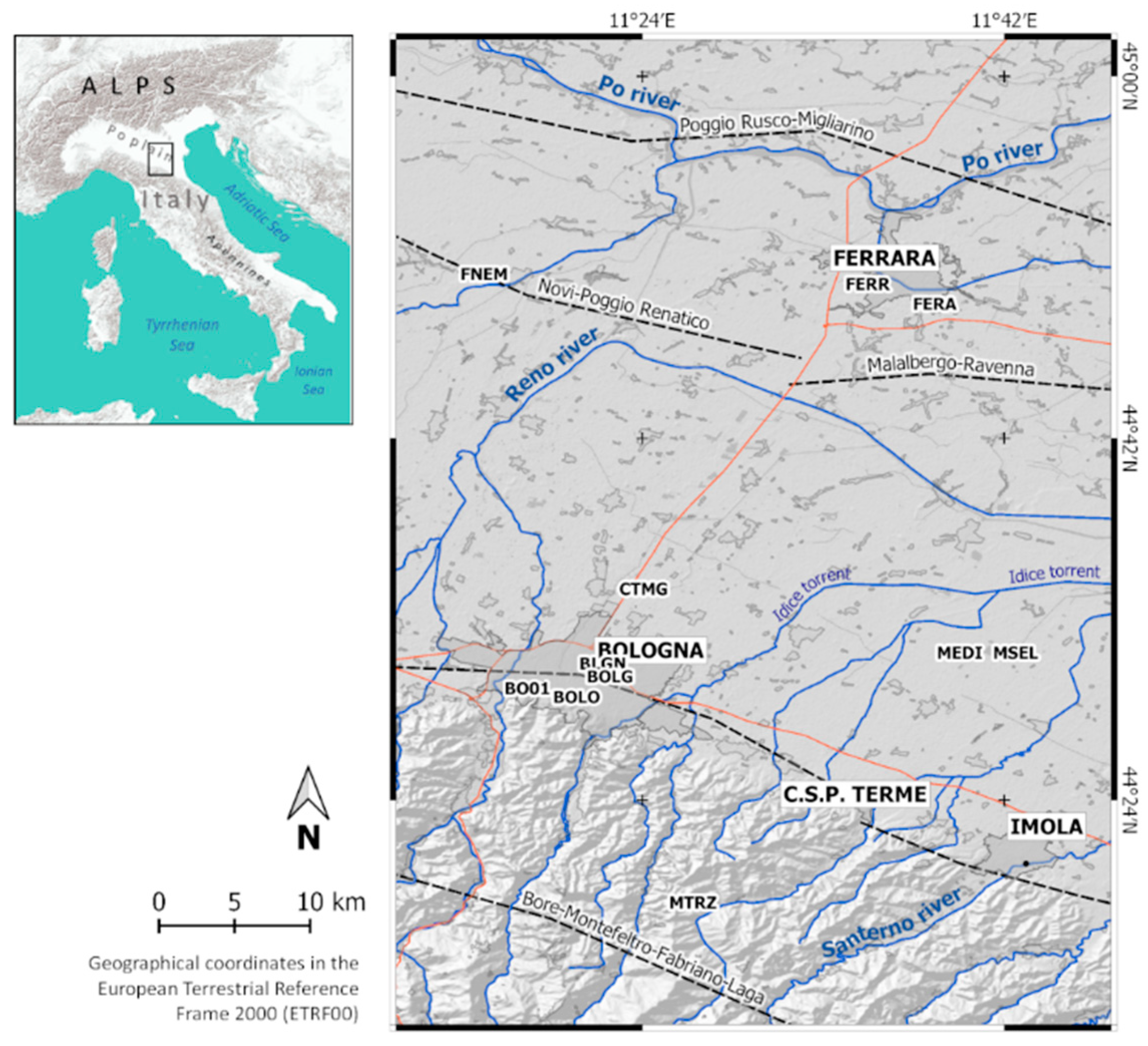
2. Study Area

This paper investigates an area of the eastern sector of the alluvial Po plain (Figure 1, inset). This area is characterized by the historical and present lowering of the ground soil due to a combination of anthropogenic and long-term geological processes. The human-induced contribution is mostly connected to the demand for the groundwater from a well-developed multi-aquifer system that started during the second half of the 20th century, in parallel with the increasing industrial activities [34,35]. A further minor human contribution has come from the extensive agricultural and zootechnical techniques and from gas exploitation [36], the latter strongly limited to the extents of productive areas. Indeed, the loading and compaction of the Holocene sediments is the main source of subsidence from natural processes in the alluvial plain, in addition to minor contributes due to deep active tectonics. As reported by [37], the modern rate of subsidence is at least an order of magnitude greater than the historical rate. The major cities included within the study area are Bologna and Ferrara, settled on areas that are characterized by very different geological settings and superficial deformation processes [37] (Figure 1).

3. Interferometric Data Processing and Analysis of GNSS Observations

In this section, main theoretical foundations for the SAR interferometry and the workflow adopted to process the S1 SAR images and observations from the CGNSS sites are discussed.

3.1. Interferogram Generation

To produce the stack of interferograms, the whole dataset of ascending and descending S1 SAR images were processed with respect to a single master image. The selection of the master image was based on minimization of the possible geometrical and temporal decorrelation effects [7,8,39]. The selection of the master image might thus have a significant role in the effectiveness of the whole procedure. The joint effects of sources of decorrelation have to be considered, with estimation of the total correlation coefficient [40],

$${\rho }_{total}={\rho }_{temp}\cdot {\rho }_{spat}\cdot {\rho }_{Doppler}\cdot {\rho }_{therm}\approx \left(1-f\left(\frac{T}{T_C}\right)\right)\cdot \left(1-f\left(\frac{B_{PERP}}{B_{PERP,C}}\right)\right)\cdot \left(1-f\left(\frac{F_{DC}}{F_{DC,C}}\right)\right)\cdot {\rho }_{therm}$$

(1)

where:

$$f\left(x\right)=\{\begin{array}{c}x , for x\le 1\\ 1, for x>1\end{array}$$

and ${\rho }_{temp}$ is the temporal correlation coefficient, ${\rho }_{spat}$ is the spatial correlation coefficient, ${\rho }_{Doppler}$ is the Doppler correlation coefficient, ${\rho }_{therm}$ is the thermal correlation coefficient, $B_{PERP}$ is the perpendicular baseline, $T$ is the temporal baseline, $F_{DC}$ the Doppler centre frequency difference between two images, and the term C is the critical one. $B_{PERP,C}$ and $F_{DC,C}$ terms do not represent limiting factors in S1 data processing being the S1 mission designed to minimize these sources of decorrelation. Then, assuming ${\rho }_{therm}$ is constant, the master is chosen where the value of ${\sum }_{i=1}^N{\rho }_{total}$ is maximized, where N is the total number of images.

The interferometric processing of data acquired using the Terrain Observation with Progressive Scan (TOPS) mode follows the approach presented by [41,42]. The interferometric operations are performed at a burst level, and thus the selection of the same swaths and bursts for the master and slave images is required. Then, the coregistration of the SAR images is performed by exploiting the precise orbit information (provided after two weeks from the acquisition time) and an external digital elevation model (DEM) of suitable accuracy and spatial resolution. After coregistration of the image pairs, the merging of adjacent bursts in azimuth direction (i.e., the deburst step) and the selection of the study area can be performed. The image pairs are then used in the generation of the stack of interferograms. Finally, the contribution of the topography to the interferometric phase must be removed, with the support of the external DEM.

3.2. PSInSAR

It is worth noting that the developed workflow for the selection of persistent scatterers and the computation of their displacement history follows the theory of the persistent scatterer InSAR technique. The basic method to identify and select persistent scatterers considers a constant velocity model for targets motion [9,39]. Once these pixels are selected, their phase history is analyzed, and only the pixels with a history similar to the functional model are included as final persistent scatterer candidates [9]. This approach can limit the application of the technique when the actual deformation model differs from that stated in the initial hypothesis. According to the StaMPS method, initial selection of the persistent scatterer candidates is performed based on amplitude analysis [11]. First, by exploiting the statistical relationship between the amplitude and phase stabilities, a high value of the amplitude dispersion as defined by [9] is used as a threshold value:

$$D_A=\frac{{\sigma }_A}{{\mu }_A}$$

(2)

where ${\sigma }_A$ is the standard deviation, and ${\mu }_A$ is the mean of the amplitude of the pixel; a value of 0.4 was suggested by [10] for such parameter. Then the phase stability of each pixel is analyzed by estimating the phase noise contribution [11] through an iterative process and checking that it does not obscure the signal and, in particular, the displacement term. Indeed, the wrapped phase of the x-th pixel and the i-th interferogram is given by the following equation:

$${\psi }_{x,i}=W\left\{{\varphi }_{D,x,i}+{\varphi }_{A,x,i}+\mathsf{\Delta }{\varphi }_{S,x,i}+\mathsf{\Delta }{\varphi }_{\theta ,x,i}+{\varphi }_{N,x,i}\right\}$$

(3)

where $W\{\cdot \}$ is the wrapping operator, ${\varphi }_{D,x,i}$ is the phase change due to displacement along the line of sight (LOS) of the pixel, ${\varphi }_{A,x,i}$ is the phase contribution due to atmospheric refraction, $\mathsf{\Delta }{\varphi }_{S,x,i}$ is the residual phase that depends on the satellite orbit inaccuracies, $\mathsf{\Delta }{\varphi }_{\theta ,x,i}$ is the residual phase due to look angle error, and ${\varphi }_{N,x,i}$ is the phase noise term [11].

The final selection of eligible persistent scatterers is performed through a statistical approach. In this step, pixels that do not have stable behavior along the period spanned by the data and/or are affected by the response from neighbouring pixels can be removed. Indeed, even if scatterers remain dominant in a specific pixel, as its characteristics can change over time, so can its response to radar signals. Such a pixel would not be considered a persistent one, and it must be discarded. Moreover, pixels adjacent to a persistent scatterer are considered to belong to the same scatterer, and the physical location corresponds to the pixel with the highest ${\gamma }_x$ (see Equation (20) in [11]). The spatially uncorrelated part of the signal is primarily due to the spatially uncorrelated part of the look angle error ($\mathsf{\Delta }{\varphi }_{\theta }^u$) and the contribution of the master (${\widehat{\varphi }}_x{}^{m,u}$). This part is estimated and subtracted from the unwrapped phase. This step is mandatory, because the spatially uncorrelated contribution can affect the wrapped phase, and thus the success of the whole unwrapping process. The wrapped phase can be written as:

$$W\left\{{\psi }_{x,i}-\mathsf{\Delta }{\varphi }_{\theta }^u-{\widehat{\varphi }}_x{}^{m,u}\right\}$$

(4)

Then, the unwrapping, performed by the method discussed in [26], yields the unwrapped phase:

$${\widehat{\varphi }}_{x,i}={\varphi }_{D,x,i}+{\varphi }_{A,x,i}+\mathsf{\Delta }{\varphi }_{S,x,i}+\mathsf{\Delta }{\varphi }_{\theta ,x,i}^c+{\varphi }_{N,x,i}-{\widehat{\varphi }}_x{}^{m,u}+2k_{x,i}\pi$$

(5)

where $\mathsf{\Delta }{\varphi }_{\theta ,x,i}^c$ is the spatially correlated part of $\mathsf{\Delta }{\varphi }_{\theta ,x,i}$, and $k_{x,i}$ is the remaining unknown integer ambiguity. The spatially correlated phase terms are estimated using temporal and spatial filtering and subtracted in order to retrieve the displacement term. Finally, the atmospheric phase can be removed.

3.3. Atmospheric Filtering

For the estimation of the tropospheric phase contribution, we used the linear phase-based model included in the Toolbox for Reducing Atmospheric InSAR Noise (TRAIN), a module developed by the University of Leeds to reduce the atmospheric noise [43,44]:

$$\mathsf{\Delta }{\varphi }_{tropo}=K_{\mathsf{\Delta }\varphi }h+\mathsf{\Delta }{\varphi }_0$$

(6)

where $\mathsf{\Delta }{\varphi }_{tropo}$ is the interferometric tropospheric phase contribution, $h$ is the topography, $K_{\mathsf{\Delta }\varphi }$ is the coefficient that relates the phase to the topography, and $\mathsf{\Delta }{\varphi }_0$ is a constant phase shift that is applied to the extent of the interferogram. The atmospheric filtering is performed in a final step of the PSI processing to remove residual and local artifact.

3.4. Vector Decomposition with Uncertainties

The LOS-oriented displacements, detected from the interferometric processing of the ascending and descending orbits, can be decomposed into the actual displacement along the North, East, and vertical directions using the procedure introduced in [45]. In general, for a satellite orbit with heading ${\alpha }_H$ the mean velocity along the LOS can be expressed following the theory of [46], where instead of the displacement, the mean velocity of the persistent scatterer is considered, without losing the validity of the discussion, as shown in the equation:

$$v_{LOS}=v_{Up}\cos \left({\theta }_{inc}\right)-\sin \left({\theta }_{inc}\right)\left(v_N\cos \left({\alpha }_H-\frac{3\pi }{2}\right)+v_E\sin \left({\alpha }_H-\frac{3\pi }{2}\right)\right)$$

(7)

where ${\theta }_{inc}$ is the incidence angle, $v_{UP}$ is the mean velocity component in the vertical direction, $v_N$ is the mean velocity component in the North direction, and $v_E$ is the mean velocity component in the East direction. Equation (7) can be adopted to project absolute velocities provided by the processing of CGNSS time series into ascending and descending slant range directions. In the present work, this procedure is used to constrain and align slant-oriented velocities to a global reference frame. This is performed prior of further decomposition analyses. In addition, from Equation (7), the propagation of uncertainties that affect the CGNSS site velocities along the North, East and vertical (up) directions can be performed to obtain the level of uncertainty of the LOS-oriented velocities:

$${\sigma }_{V_{LOS}}^2={\cos }^2{\theta }_{INC}\cdot {\sigma }_{V_{UP}}^2+{\sin }^2{\theta }_{INC}\left[{\cos }^2\left({\alpha }_{\pi }-\frac{3}{2}\pi \right)\cdot {\sigma }_{V_N}^2+{\sin }^2\left({\alpha }_{\pi }-\frac{3}{2}\pi \right)\cdot {\sigma }_{V_E}^2\right]$$

(8)

Following the theory proposed by [46], the sensitivity to displacement oriented along the North-South direction is very low. The S1 orbit is designed with a mean incidence angle of approximately 37° and a heading angle of 190°. Given the acquisition geometry, the sampling of the actual displacement oriented along the North-South direction by the slant looking shows a sensitivity of −0.10. Consequently, the vector decomposition procedure aims to compute the displacement along the Earth-West (E) and vertical (Up) components from the ascending and descending passes only. Using the matrix notation, the expression given in the following equation holds:

$$\left[\begin{array}{c}{v}_{UP}\\ v_{EAST}\end{array}\right]=A^{-1}\cdot \left[\begin{array}{c}{v}_{LOS}^{ASC}\\ v_{LOS}^{DESC}\end{array}\right]$$

(9)

where:

$$A=\left[\begin{array}{cc}\cos \left({\theta }_{ASC}\right)& \sin \left({\theta }_{ASC}\right)\cos \left({\alpha }_{H,ASC}\right)\\ \cos \left({\theta }_{DESC}\right)& -\sin \left({\theta }_{DESC}\right)\cos \left({\alpha }_{H,DESC}\right)\end{array}\right]$$

Note that ${\theta }_{ASC}$ has a negative value because of its counterclockwise counting. From Equation (9), the variance–covariance matrix of decomposed velocities can be expressed through the uncertainty error propagation law as:

$$C_{V_{decomp}}=A^{-1}{C}_{V_{LOS}}{\left(A^{-1}\right)}^T$$

(10)

Equation (10) allows the computation of uncertainty level to be assigned at velocities along the Earth-West (E) and vertical (Up) directions after the decomposition of slant-oriented velocities.

3.5. Accuracy Assessment with Error Propagation Analysis

To provide an accuracy assessment of PSI-derived velocities a comparison with CGNSS time series can be used. This comparison could be performed at the level of time series projected along a common direction or by using decomposed velocities. The comparison of average annual velocities from regression analysis applied to PSI and CGNSS time series could be poorly sensitive to unmodelled effects. However, its significance increases when comparing linear trends of slow ground deformation phenomena.

The approach followed in the present paper uses the error propagation law. As reported in Section 3.4, a level of uncertainty can be assigned to the decomposed PSI velocities and used to establish the statistical significance of the comparison with CGNSS actual velocities. This approach requires: (a) the assessment of uncertainties introduced by the alignment of PSI-derived slant velocities to the reference frame and (b) the error propagation analysis to obtain uncertainties of decomposed PSI velocities in the vicinity of a CGNSS sites used in the error assessment procedure. The decomposition procedure requires a preliminary sampling and averaging of PSI-based velocities over regular grid for ascending and descending products. Then, during the step (b), uncertainties linked to averaging procedure of slant velocities and decomposition procedure (the latter using Equation (10)) propagate. The comparison between PSI and CGNSS velocities could be therefore complemented by the uncertainty level.

3.6. GNSS Data Processing Strategy

The absolute reference frame for the differential displacement provided by the PSI methodology was defined using a network of CGNSS sites that are unevenly distributed within the study area. Moreover, CGNSS time series can provide fundamental information about the tectonic and geodynamic behaviors of the region and help in the understanding of the superficial kinematic phenomena. Unfortunately, CGNSS sites belonging to international networks are usually a limited number over an area of interest and stations from other positioning services could be of interest in the validation processes. Figure 1 shows the distribution of the CGNSS stations used in this work to provide a constraint to the global reference frame and reference absolute velocities at sites used in the assessment of PSI-derived velocity. These CGNSS sites are managed by different public and private agencies for different purposes, and for this reason, they are not evenly distributed, and the observation time spans might differ. Some sites were developed for scientific investigations by public research authorities, while others make up part of the national services for real-time positioning. However, [47,48] demonstrated that CGNSS sites designed and realized for technical operations do not introduce noise into the data recorded, with respect to sites used for scientific applications.

In the present study, we have considered only the CGNSS sites located in the study area with observations acquired between 1 March 2015, and the end of 2019 were processed using the GAMIT-GLOBK software package (Herring et al. 2018a, b). In particular, the processing strategy excluded the sites with data from <2.5 years and efficiency <50% (i.e., number of days with regular observations with respect to the whole period of observation). During the processing, a loose constraint approach (i.e., 100 m) was applied to a-priori coordinate of each site, while tight constraints were used for the precise ephemerides and the Earth Orientation Parameters. The FES2004 ocean-loading model [49] and an atmospheric propagation delay based on the global mapping function [50] were used in addition to the absolute antenna phase center model provided by the International GNSS Service for satellites and ground stations. At the end of the first step of the processing, the daily solutions were loosely constrained using the GLOBK package [51] to the European Terrestrial Reference Frame (ETRF2014; [52]) using a seven-parameter Helmert transformation, where the differences between the positions of the 14 International GNSS Service stations surrounding the study area were minimized [53]. The daily time series of the North, East and vertical components estimated was modelled as:

$$y_j\left(t_i\right)=D_k+v_k{t}_i+{\displaystyle \sum }_{k=1}^N{d}_{\mathrm{jk}}H\left(t_i-T_k\right)+{\displaystyle \sum }_{k=1}^M\left(A_{1k}\cos \left(\frac{2{\pi t}_i}{P_k}\right)+A_{2k}\sin \left(\frac{2{\pi t}_i}{P_k}\right)\right)+{\epsilon }_k\left(t_i\right)$$

(11)

where j represents the North (j = 1), East (j = 2) and vertical (j = 3) components. Assuming a linear trend of displacement in the time series within the analyzed time span, the initial position (D) and velocity (v) obtained from an ordinary least squares linear regression analysis were used to model the long-term trend. The N discontinuities due to instrumental changes and seismic events that occur near the sites are modelled with the d_jk terms, ε_k(t_i) is time-dependent noise, and A_1k and A_2k are the amplitudes of the M (M ≤ 5) seasonal signals with period P_k. During the first phase of the analysis, only the initial position (D_k), velocity (v), discontinuities (d_ki), and noise (ε_k(t_i)) were estimated by a weighted least-squares method. To obtain a residual time series, a model of the motion was computed using the parameters estimated and, successively, this motion was removed from the time series. Residuals were used to compute the standard errors of the linear regression analysis and, successively, analyzed using a non-linear least-squares technique to estimate the spectra, following the Lomb–Scargle approach [54,55]. The spectrum of each component was analyzed to estimate the period, P, of the five (statistically meaningful) principal signals in the interval between 1 month and half of the observation time span. Periodicities were therefore used in Equation (11) to estimate discontinuities, the intercept, and velocities, with amplitude $A_k=\sqrt{A_{1k}^2+A_{2k}^2}$ and phase $\varphi =arctg\frac{A_{2k}}{A_{1k}}$ for each component.

4. Available Data and Processing Workflow

The interferometric processing discussed here was performed using free and open-source tools and software. Indeed, the complete workflow is based on the sequential use of the software packages of SNAP for interferograms generation, and StaMPS to process persistent scatterer time series, with the following reduction of the atmospheric effects by the model discussed in Section 3.1 and included in TRAIN.

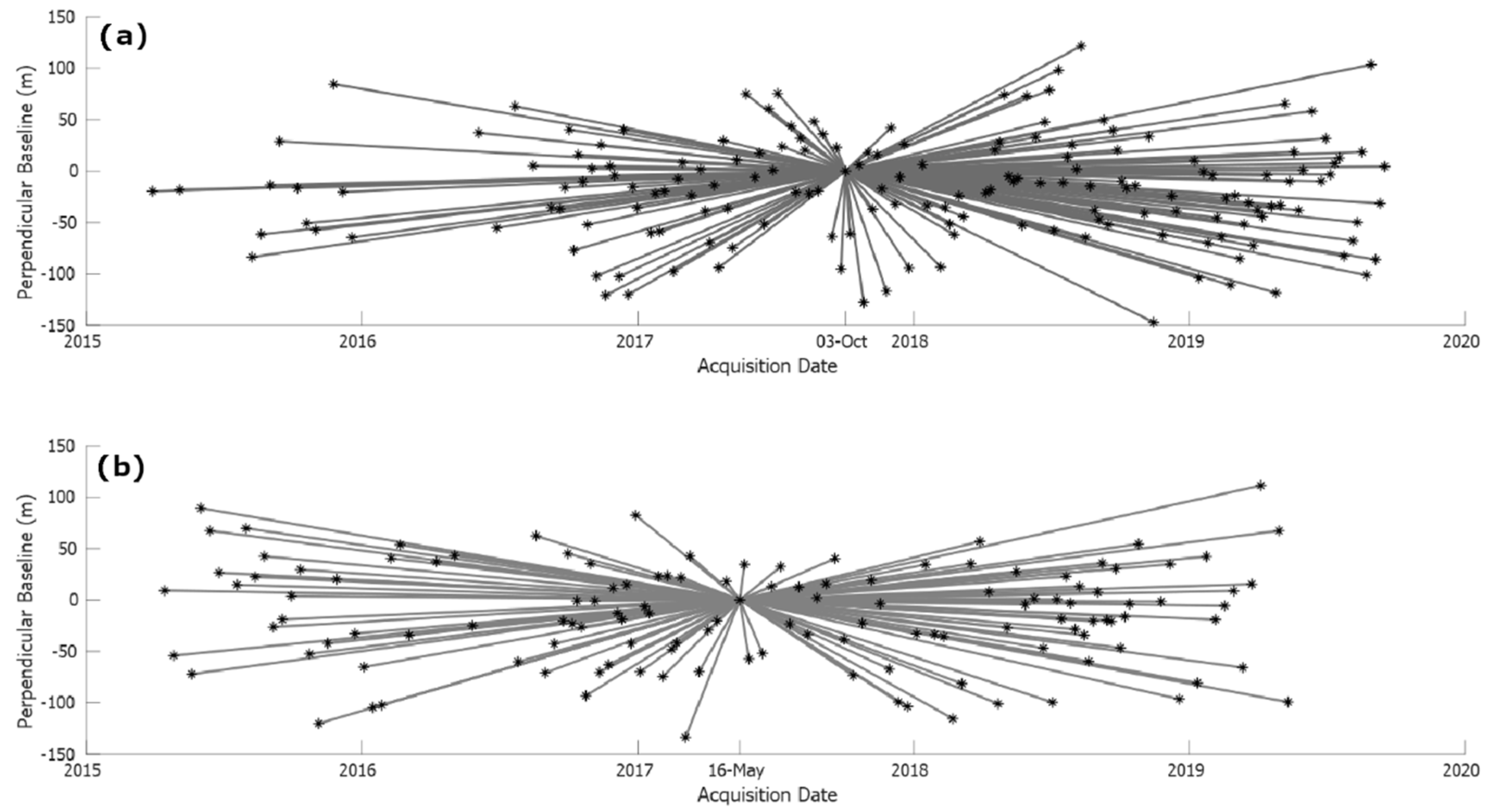
4.1. Sentinel-1A and -1B Radar Dataset

The satellite radar data used in this study was delivered under the Copernicus program and acquired by the S1A and S1B platforms placed in near-polar Sun-synchronous orbits, with inclination of 98.18° at an altitude of 693 km. Each satellite has a repeat cycle of 12 days, while for joint use of S1A and S1B, this is reduced to 6 days. Each satellite has a C-band radar with a frequency range of 4–8 GHz and a wavelength range of 37.5–75.0 mm. The acquisition is carried out with the TOPS acquisition mode, in which the antenna beam is steered in terms of both range (to acquire data from three sub-swaths, as in ScanSAR mode) and azimuth (from backward to forward for each sub-swath). As a consequence, the targets are illuminated by the entire azimuth antenna pattern, thus strongly reducing the scalloping effect and leading to constant signal-to-noise ratio and ambiguities along the azimuth direction. The main drawbacks are the reduced spatial resolution along the azimuth direction caused by the fast azimuth beam steering and the need for extremely precise coregistration. Single Look Complex (SLC) images acquired by the Interferometric Wide (IW) acquisition have been downloaded from the Sentinel Scientific Data Hub (scihub.copernicus.eu) of the Copernicus Open Access Hub.

The IW SLC images have a nominal resolution of 20 m × 5 m (azimuth × range, respectively) and a ground swath width of 250 km. Moreover, they are composed of three sub-swaths (IW1, IW2, IW3) and by three images in single polarization and six images for dual polarization. Each of the sub-swaths has a different mean incidence angle (IW1, 32.9°; IW2, 38.3°; IW3, 43.1°) and consists of a series of bursts in the azimuth which partially overlap in both directions to guarantee the continuity of the image spatial coverage.

In the present study, the ascending and descending Sentinel-1A and Sentinel-1B IW SLC products reported in

Table 1. The Sentinel-1 datasets used in this study.

Orbit	Track	Number of S1 Images	Master Image Acquisition Date	Period		Number of Bursts (n)	Sub-Swath	Mean Incidence Angle (°)
				Start	End
Asc.	117	171	3 October 2017	30 March 2015	17 September 2019	5	IW2	38.3
Desc.	95	132	16 May 2017	15 April 2015	12 May 2019	5	IW1	32.9

were selected for the successive processing. The temporal and perpendicular baselines between the master and the slave images are reported in Figure 2.

4.2. Software

The Sentinel Application Platform is an architecture that is provided by the ESA and incorporates all the necessary tools to ensure visualization and processing of the Sentinel mission data. The Sentinel-1 Toolbox includes the functionalities for the processing of both ESA (e.g., Sentinel-1, ERS-1, ERS-2, Envisat) and third party (e.g., Cosmo SkyMed, Radarsat-2, TerraSAR-X, ALOS PALSAR) SAR missions. In particular, the SNAP TOPSAR capabilities allow InSAR processing for integration with the StaMPS package, to provide full PSI time series analysis [27]. StaMPS is a software package that was developed by Stanford University (Stanford, USA), University of Iceland (Reykjavík, IS), Delft University (Delft, NL), and University of Leeds (Leeds, GB) that implements the PSInSAR method to extract ground displacements from time series of synthetic aperture radar acquisitions. StaMPS works even in the case of non-steady deformation [56]. The TRAIN tool is available in StaMPS for reduction of the atmospheric noise. In addition to the phase-based linear correction used in this work, TRAIN includes several other models: phase-based power-law correction; spectrometer correction (Moderate/Medium Resolution Imaging Spectrometer [MODIS/MERIS]); weather model correction (European Reanalysis-Interim [ERA-I]; Modern-Era Retrospective Analysis for Research and Applications [MERRA/MERRA-2]; Generic Atmospheric Correction Online Service [GACOS]; Weather Research and Forecasting model). See [43,44] for further details.

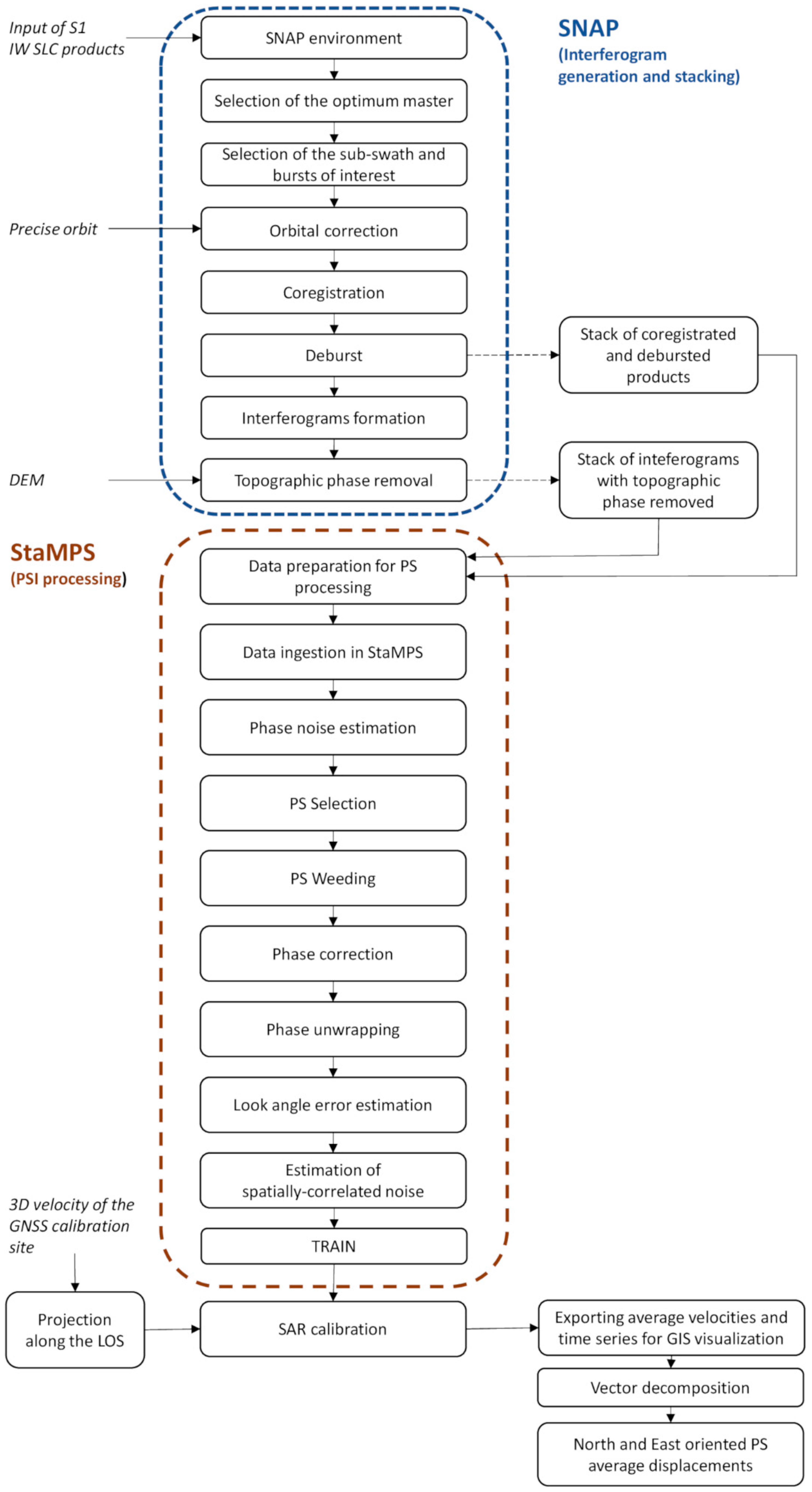
4.3. The Processing Workflow

The SNAP–StaMPS workflow used in the present study is summarized in Figure 3 and further commented on in this section, with details of the single steps performed during the processing.

The SNAP InSAR processing strategy used in the present study includes all the necessary steps for the preparation of products needed for persistent scatterer processing in StaMPS, which are, in particular:

• Master image selection. The Optimal InSAR master selection tool is used, which implements the theory reported in [40];
• Product splitting. For all of the SLC data, the same sub-swath and bursts have to be selected, to ensure the success of the co-registration;
• Orbital correction. The Sentinel precise orbit files are applied to all of the products, with these files made available approximately 20 days after acquisition, and automatically downloaded during the processing;
• Coregistration. This step is performed exploiting the Back Geocoding operator;
• Deburst. In this step, adjacent bursts are merged in the azimuth direction according to their zero-Doppler times, with resampling to a common pixel spacing with the S1 TOPS Deburst operator (VV polarisation selected);
• Interferogram formation. Computation of the complex interferograms;
• Topographic phase removal. The topographic phase is estimated and subtracted from the interferograms with the shuttle radar topography mission (SRTM) 3 arc-seconds DEM downloaded by the software. During this step, the output file contains the topographic phase band, the elevation band, and the orthorectified positions as latitude/longitude;
• StaMPS export. In this step, the folder structure required by StaMPS is prepared, starting from the stack of coregistered and deburst products and the stack of interferograms free from the topographic phase contribution. The export is performed using the PSI/SBAS interferometric tool.

The processing parameters for PSI analysis by StaMPS are set using the available mt_prep_snap script. Parameters like the amplitude dispersion ($D_a$) and the number of overlapping pixels in the azimuth ($n_a$) and range ($n_r$) are left as default ($D_a=0.4$; $n_r=50$; $n_a=200$), while the number of patches is selected depending on the computational characteristics of the computer. As an example, for the descending orbit, five patches were produced, both for azimuth and range. The amplitude dispersion parameter was left as default because, due to the prevalence of vegetated land cover in the study area, no improvements were found increasing its value as total number of candidate PS.

The stack of interferograms is processed using MATLAB procedures implemented in StaMPS, complemented by linear-phase-based tropospheric corrections using TRAIN [43,44]. In more detail, this includes:

• Data loading. Preparation of the dataset required for the PSI processing;
• Phase noise estimation. Estimation of the phase noise for each candidate pixel in every interferogram;
• Persistent scatterer selection. Selection of eligible persistent scatterer pixels on the basis of noise characteristics;
• Persistent scatterer weeding. Discarding of noisy persistent scatterers or persistent scatterers affected by signal contributions from neighbouring elements;
• Phase correction. Correction of the wrapped phase for spatially uncorrelated look angle error, and merging of the patches of interest;
• Phase unwrapping;
• Spatially correlated look angle error estimation. This error is due to errors in the DEM and incorrect mapping of the DEM into the radar coordinates;
• Estimation of other spatially-correlated noise.

At the end of StaMPS processing, the TRAIN linear phase-based correction is applied. Further details about these steps can be found in the reference StaMPS/MTI Manual [56,57].

At this stage, the user can select a reference area/site and introduce an average velocity for it (usually known from the CGNSS data). The whole persistent scatterer dataset will be referred to this reference velocity. However, by default, StaMPS uses the whole extent as a reference area. The mean of the interferometric unwrapped phases from all the persistent scatterers is computed, and its value is set to zero. In this way, the mean stability behavior across the entire scene is assumed. This step is shown in Figure 3 as the SAR calibration and introduces a constraint to a global reference frame. Whenever data have to be visualised in a GIS environment, a vector shapefiles format can be exported, which contains the coordinates of each persistent scatterer and an attribute table including the time series of slant-oriented displacements for relevant epochs and the average velocity from a least squares regression analysis. We added a MATLAB procedure for vector decomposition and computing of the vertical and East-West oriented displacement. In the decomposition procedure, the variation of the incidence angle all over the study area was considered and the correct value for each resolution cell was used.

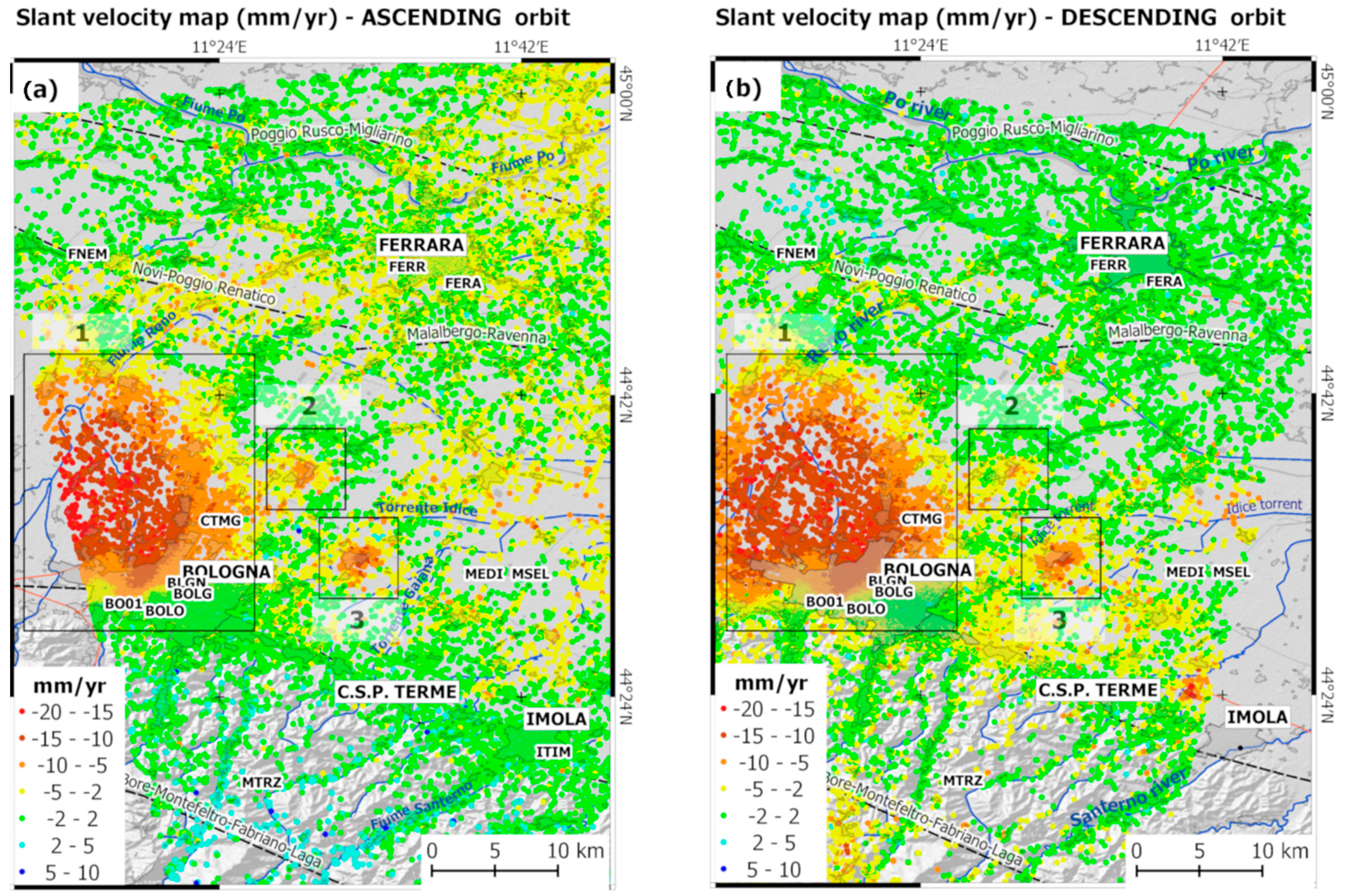
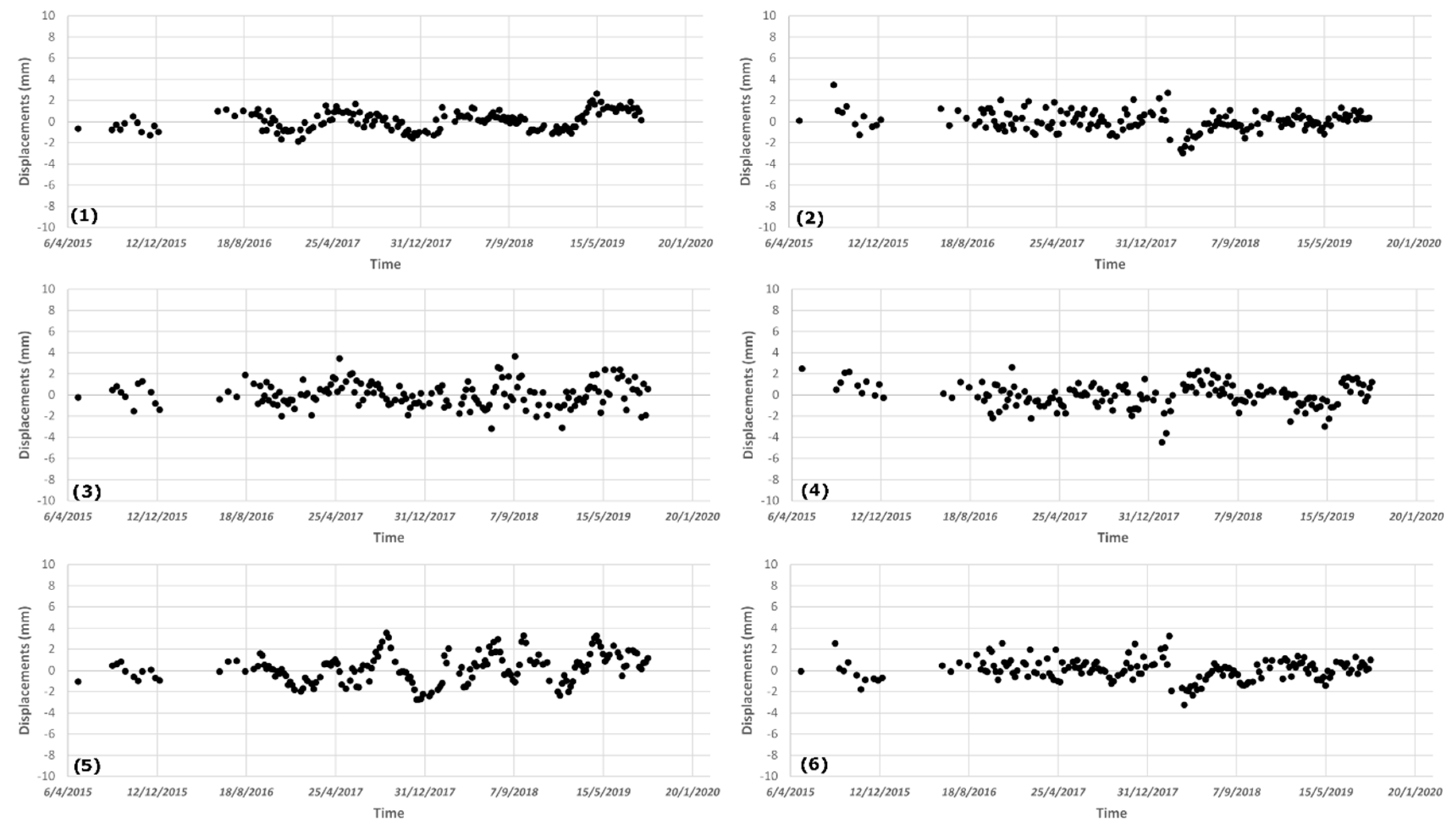
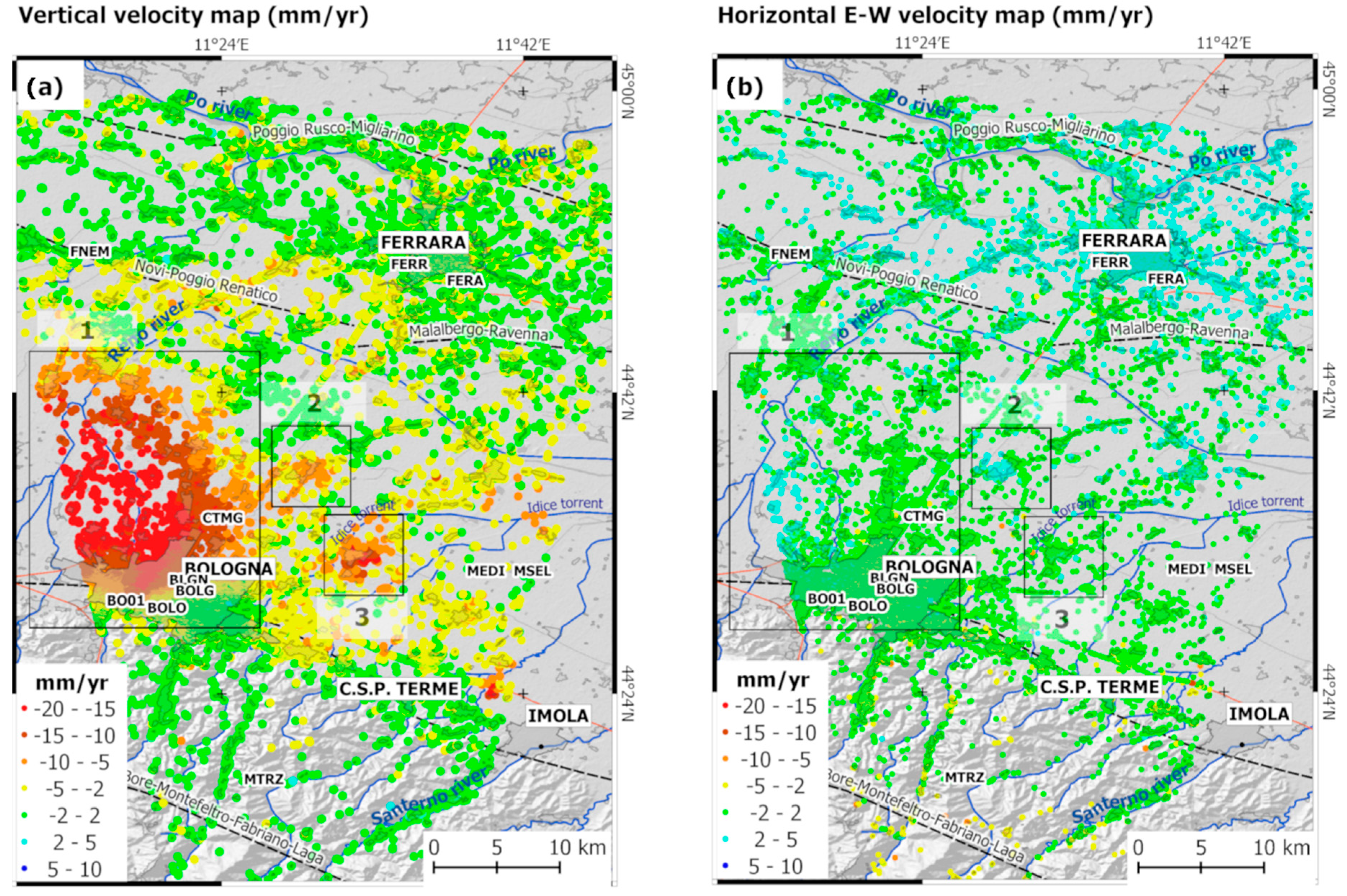
5. Results

The interferometric processing of S1 SLC images acquired from ascending and descending orbits generated a geocoded LOS velocity map over the study area. To filter out scatterers that showed low temporal coherence, we assumed as coherent pixels those characterized by Da < 0.4. As indicated, the displacements are initially computed under the hypothesis of mean stability behavior across the entire scene. Then, to align the ascending and descending LOS velocities to a common reference frame, we used the local deformation trend provided by the processing of a single CGNSS station included in the study area during an overlapping period. In particular, the BOLG CGNSS station was chosen as the reference by a criterion based on the time length of the series, number of days with regular observations with respect to the whole period of observation and quality of the monument used in the antenna installation. BOLG is part of the EUREF Permanent GNSS Network. It guarantees a reliable constraint to the global reference frame (see Figure 1). The velocities processed at the BOLG site using Equation (11) and referred to an observation time span that overlaps with the interferometric dataset are: $V_{UP}=-1.0\pm 1.2\mathrm{mm}/\mathrm{yr}$, $V_E=0.3\pm 0.5\mathrm{mm}/\mathrm{yr}$ and $V_N=4.6\pm 0.5\mathrm{mm}/\mathrm{yr}$. The residual horizontal components (North and East) are estimated by removing the Eurasian plate movements modelled with the parameters provided by [52]. The CGNSS velocities projected along the ascending and descending LOS directions are processed with uncertainties according to Equations (7) and (8), respectively. The following values are obtained: $V_{LOS,ASC}=-1.4\pm 0.9\mathrm{mm}/\mathrm{yr}$, $V_{LOS,DESC}=-1.1\pm 1.0\mathrm{mm}/\mathrm{yr}$. Figure 4 illustrates the LOS-oriented velocity maps within the study area.

The uncertainties introduced by the alignment procedure arise from the linear combination of errors characterizing the average velocities from CGNSS and PSI time series adopted for alignment purposes. The uncertainty included in the average velocity of radar targets located in the vicinity of BOLG station could be quantified by a statistical analysis applied to the group of selected PSI time series used. In particular, a sample of 36 slant velocities in both orbits has been used and averaged to find reliable average values to be aligned with slant projected CGNSS velocities. Figure 5 provides a sample of ascending PSI time series for targets located in the vicinity of BOLG reference site. The uncertainty of average slant velocities could be placed at 0.1 mm/yr.

As shown by time series of Figure 5, the scattering of points displacements is within a couple of mm among the epochs. Successively, uncertainties introduced by the alignment procedure are transferred to single slant velocities within the study area and will be further propagated in the final error propagation analysis.

The LOS-oriented velocity maps in Figure 4 show deformation phenomena to different geographic extents. It can be noted, three zones (1, 2, and 3 in Figure 4) where the ground deformation is higher than the surrounding areas. As pointed out by a number of studies carried out in this area [32,47,48,58], the displacement pattern is mainly related to lowering of the ground soil due to mainly anthropogenic causes. Previous studies in the area that were based on satellite radar interferometry did not perform decomposition analysis from ascending and descending slant displacements. However, a contribution from horizontally oriented displacement cannot be excluded a priori. This assumption fails in the case of phenomena characterized by the horizontal displacement of the same order as the vertical one, as detected by previous studies in the Po plain area [47,48,53,58]. These investigations reveal horizontal and vertical displacement rates from GNSS data of comparable magnitude. Thus, to achieve full knowledge of the superficial velocities field as seen by the SAR acquisition geometry, there is the need for vector decomposition analysis from ascending and descending velocity maps acquired in the slant geometry complemented by the error propagation analysis (see paragraph Section 3.4).

Before the decomposition procedure can be performed, the ascending and descending dataset are sampled over a common grid with a cell size comparable with the spatial resolution of the Sentinel-1 data. A grid of 20 m × 20 m in the ground range is selected and Equation (9) is used to compute the velocities along the vertical (up) and East-West directions for cells with at least 1 persistent scatterer included in both orbits. After the decomposition procedure with a 20-m grid size, vertical and horizontal velocities for 111,306 targets were obtained. The use of larger grid size in the decomposition analysis produces a decrease in the cells associated with decomposed velocities, and a smoothing effect on the resulting decomposed velocities. For instance, a sampling grid size of 30 m × 30 m corresponds to a reduction of the final cells by 10%. The results obtained from this decomposition procedure are shown in Figure 6, where the displacement oriented in the vertical (up) and East-West directions are shown.

In particular, Figure 6a shows the significant vertical deformation patterns over a wide area in the western sector of the metropolitan area of Bologna (area 1), where vertical rates of up to 20 mm/yr can be seen over an extent of ~200 km². The horizontal velocity pattern shows increasing eastern movement in the same area where the greatest subsidence velocities are seen. These data suggest that the subsidence processes also involve the horizontal displacement.

Velocity maps visible within the areas 2 and 3 differ and an insight will be provided with the aim to show the ability by the maps to inform on ground deformations even by using decomposed velocities. Figure 7 shows the vertical and horizontal velocity maps within the area 2, located in the municipality of Minerbio (district of Bologna).

As visible in Figure 7a, the area exhibits subsidence rates up to 10 mm/yr. Moreover, a prevalent East-West component is well depicted in Figure 7b over a delimited area. In this area, an industrial activity (gas storage in depleted deposits) takes place. However, the authors do not have any other evidence for this relationship and detailed study of the causes of such superficial deformation field is far from the aims of this study. Similarly, Figure 8a,b, shows vertical and horizontal velocity maps processed in the municipalities of Budrio (area 3).

In the remaining part of the investigated areas the horizontal velocity pattern shown on Figure 6b indicates widespread and eastward movement (i.e., positive values) in the range of a few mm/yr, especially in the northern area, where the city of Ferrara is located. The eastern sector of this area was stricken by the seismic events in May–June 2012. This area below the Po plain sedimentary cover is characterized by a buried arcuate thrust system and growth folds related to the Apennines chain [59], the principal lineaments of which are also shown in Figure 6b. The moderate uplift in this area (Figure 6a) might be connected to the tectonic movements of the buried Apennines chain, as suggested by several studies for the eastern movements shown in Figure 6b [60]. Finally, minor contributions to the eastward displacement might derive from actual displacements along the North direction, which would contribute to a lesser extent in the slant direction and in successive decomposition analysis.

To provide quality assessment for the vertical and horizontal velocity maps after the decomposition procedure, the rates produced by the PSI-based analysis were compared with GNSS measurements relevant to the period of the InSAR analysis. The CGNSS observations and time series were specifically processed here for this purpose. All measurements are complemented by the uncertainty levels (provided as standard deviations) and, based on the procedure discussed in Section 3.4 and Section 3.5, the error propagation analysis is performed to provide errors in the final comparison between GNSS and decompose PSI velocities. The results are given on

Table 2. Results of the comparisons between the velocities at the GNSS sites and the average persistent scatterer interferometry velocities for a minimum set of five persistent scatterers located around the CGNSS site at a distance ≤500 m.

CGNSS Site Code	GNSS Velocity (mm/yr) with st. dev.		PSI Average Velocity (mm/yr) with st. dev.				Comparison (GNSS – PSI; mm/yr) with st. dev.
	East	Up	East	Up	#PS	SD (m)	East	Up
BLGN	−1.5 ± 0.2	−7.6 ± 0.8	−1.2 ± 0.1	−8.1 ± 0.1	13	50	−0.3 ± 0.2	0.5 ± 0.8
BOLO	−0.4 ± 1	−1.9 ± 2	0.7 ± 0.1	−1.56 ± 0.1	7	50	−1.1 ± 1.0	−0.3 ± 2.0
BO01	0.7 ± 0.3	−4.0 ± 1.3	0.1 ± 0.1	−3.6 ± 0.1	10	100	0.6 ± 0.3	−0.4 ± 1.3
CTMG	−0.9 ± 0.8	−12.8 ± 1.6	−0.4 ± 0.1	−13.2 ± 0.1	14	100	−0.5 ± 0.8	0.4 ± 1.6
MTRZ	0.5 ± 1	−1.7 ± 1.8	−1.0 ± 0.2	−0.9 ± 0.1	2	500	1.5 ± 1.0	−0.8 ± 1.8
MEDI	1.0 ± 0.4	0.2 ± 1	0.4 ± 0.1	−1.5 ± 0.1	11	500	0.6 ± 0.4	1.7 ± 1.0
MSEL	0.6 ± 1	−1.3 ± 1.6	0.4 ± 0.1	−1.5 ± 0.1	12	500	0.2 ± 1.0	0.2 ± 1.6
FNEM	1.2 ± 0.8	−1.5 ± 2.4	1.4 ± 0.1	−1.3 ± 0.1	24	100	−0.2 ± 0.8	−0.2 ± 2.4
FERR	0.5 ± 0.7	0.1 ± 1.7	2.2 ± 0.1	−1.1 ± 0.1	9	50	−1.7 ± 0.7	1.2 ± 1.7
FERA	0.6 ± 1.1	−4.3 ± 2.1	1.9 ± 0.1	−2.2 ± 0.1	6	50	−1.3 ± 1.1	−2.1 ± 2.1

#PS, number of averaged persistent scatterers; SD, Sampling distance around the CGNSS sites to achieve the minimum of five persistent scatterers needed to compute the averages.

.

In this comparison, the PSI-based velocities were computed as the average values from a minimum of five persistent scatterers located in the vicinity of the GNSS site. A circle area with a 50-m radius was used to sample and average the persistent scatterer velocities. To reach the minimum number of required persistent scatterers, the search radius was increased 50 m until the required number of persistent scatterers was achieved. Table 2 shows the number of averaged persistent scatterers and the resulting sampling distance used around the CGNSS sites. These data reported in Table 2 show differences between the GNSS and PSI-based velocities of <±2 mm/yr within the reference period, with larger values detected for the East component for the GNSS site of FERR, and in the vertical (up) component for FERA. FERR and FERA are in the urbanized area of Ferrara, at a distance of about 40 km from the reference site. This distance might have a role. Table 2 shows levels of uncertainties <2 mm/yr in the majority of comparisons.

6. Discussion

The processing of the full ascending and descending S1 radar data and the use of contemporary GNSS observations provided the complete workflow based on PSI analysis and combined SNAP–StaMPS open-source software for ground deformation monitoring. The uncertainty levels introduced by the calibration procedure were also estimated, and the comparison with the velocities provided by a limited number of GNSS sites provided an assessment of the reliability for depicting the displacement field over an area affected by subsidence phenomena. In particular, the contemporaneity of the ascending and descending SAR data and the GNSS observations used in the present study offered us the opportunity to perform a careful calibration procedure with respect to a global reference frame, and for decomposition analysis with successive assessment of the ground deformation phenomena. A similar approach can be found in [28,29], where the PSI velocities from dual orbits were aligned and then the SAR velocities were corrected using the GNSS values. In [61], a S1 descending orbit, dataset was also processed, and the results were combined with in-situ measurements, such as groundwater and GNSS measurements, for more complete interpretation of the data. However, these previous studies based on S1 data lack contemporaneity between the datasets, and none of them explored the vertical and horizontal displacements fields with calibrations in an absolute reference frame, followed by assessment of the accuracy of the uncertainties.

Moreover, the processing workflow of the S1A and S1B data using open-source tools and then the vector decomposition procedure offers some points of discussion. As shown in Figure 5, the SNAP–StaMPS workflow provided a final persistent scatterer time series that can depict linear trends and periodical signatures along the slant direction with a points dispersion of few mm, with no further filtering procedures. After the persistent scatterer time series was processed, we selected a CGNSS site with reliable time series to align the persistent scatterer velocities from single orbits in an absolute reference frame (ETRF2014).

From the analysis of the reference site 3D GNSS time series of BOLG site, we found a propagated uncertainty level on the LOS-projected velocities at the millimeter level, which further propagates during the decomposition in the vertical (up) and East-West velocities. Such propagated errors are reported in Table 2. The comparison between CGNSS and PSI-derived velocities allowed to define differences of 2 mm/yr in worst cases with uncertainties at mm/yr. In this computation, the incidence angle must be referred to the area where the reference site is placed. The persistent scatterer time series appeared less reliable at the beginning of the reference period, when only the S1A data were available, and a void of data was found in the first half of the year 2016, due to the lack of S1 radar images in the repository used.

The use of GNSS time series processed for even longer time periods in comparison with PSI-derived series is suitable for accuracy assessments. This is due to long-term fluctuations which could be not completely detected by the period of the satellite passages. For this reason, the use of CGNSS velocities referred to different time spans could therefore affect the calibration procedure. The use of GNSS velocities available at the relevant time is therefore advised. Nevertheless, a comparison of GNSS and PSI techniques based on average annual velocities could be poorly sensitive to noises and unmodelled effects. To remove part of these noises, a comparison at the level of time series of displacements should be used. In Figure 9 the LOS-oriented ascending time series for a single target (black dots, see the PS time series number 6 in Figure 5) is compared with the CGNSS positions projected along the LOS. CGNSS are reported for the full time series (grey dots) and for a subset of points sampled at the time of satellite passages (red dots). An epoch-by-epoch comparison could be assessed by the root mean square error (RMSE). The RMSE for comparison of series represented in Figure 9 is 2.9 mm. This is mainly due to periodic fluctuations in the CGNSS time series that are not clearly visible in the response from radar target.

The linear phase-based model adopted in the present study to estimate the atmospheric phase contribution is shown to be suitable for mapping deformation in the study area. In particular, the atmospheric corrections processed for the interferograms affected the hilly area that was part of the central Apennines. After the decomposition, this area shows null vertical deformation rates, with only delimited areas characterized by very small positive rates (Figure 6, southernmost sector). This behavior is consistent with the theories related to the tectonics of the Apennine chain. Residual horizontal velocities visible on Figure 6 in correspondence with the hilly area are mostly due to slope instabilities. Removal of the atmospheric phase with more complex models included in TRAIN could be the objective of further studies.

The workflow is revealed to be useful in the detection of deformation phenomena at the millimeter level, like those affecting the Po Plain sedimentary basin. The spatial and temporal variability of the ground deformation driven by anthropogenic causes, such as gas and groundwater exploitation, might be significant, and this dual approach based on GNSS and InSAR offers a solution. A study of the spatial distribution of the phenomena is also necessary, especially when the techniques adopted have an important difference in terms of the spatial distribution: the single point for the GNSS measurements and a relatively large number of persistent scatterers on the ground for the SAR technique. For these reasons, we processed the same observation time span (2015–2019) for the GNSS and SAR observations, and the comparison between the results obtained shows good agreement between the vertical and horizontal (East-West) velocity values (Table 2). Moreover, the use of dual-orbit radar data for subsidence studies might be a requirement for the S1 satellites that are designed to work with a wider look angle with respect to past sensors, and that are less sensitive to actual vertical motion.

The workflow based on PSI analysis and combined SNAP–StaMPS open-source software has some drawbacks. The processing was time demanding using computers equipped with Intel Core i7 and 24Gb of RAM memory. The processing of ascending and descending dataset in the investigated areas took a couple of months with the majority of the processing time (roughly the 90%) used by SNAP. However, computing can be fastened using high-performance or cloud computing. The open code of StaMPS represents a positive point, and the users are able to introduce personalized routines, as we did in the calibration and vector decomposition steps.

The ground deformation map produced in the present study updates previous investigations commissioned by the Regional Agency for Environmental Prevention, on behalf of the Emilia-Romagna Region. Such studies were initially based on traditional topographic surveying [33]. From 2005, single-orbit SAR interferometry based on radar images provided by ERS, Envisat and Radarsat satellites was used to depict the subsidence phenomena over the area, thus assuming a negligible horizontal motion. These previous studies provided updates up to the year 2016 [62] and a reliable benchmark for the present investigations, even though no studies based on dual-orbit and vector decomposition are available.

The maps of Figure 6, Figure 7 and Figure 8 depict the current subsidence phenomena in the metropolitan area of Bologna, in addition to ground deformation phenomena that affect the nearby settled areas. This might represent a recent update on the modern subsidence rates, and a valuable tool for stakeholders involved in finding countermeasures to land subsidence after the continuous reduction in the amount of groundwater pumped by supply stations located within the study area [63].

7. Conclusions

In this study, we presented a PSI-based workflow to process dual-orbit S1 radar data with open-source tools complemented by the use of GNSS observations as constraints for the global reference frame and final accuracy assessment of the vertical and East-West oriented velocity maps.

The workflow allowed the investigation of ground deformation due to subsidence phenomena over large extents of Emilia Romagna (Italy). The combined use of the SNAP and StaMPS processing tools offers an opportunity for users who are interested in processing freely available S1 radar images with calibration of velocity maps and use of algorithms included in TRAIN for the atmospheric phase removal. We have added a procedure to process contemporary CGNSS site velocities to refer differential LOS-projected velocities provided by the InSAR approach to the modern ETRF2014, and an algorithm for decomposition analysis at preferred spatial resolution, with successive accuracy assessment carried out at 10 CGNSS sites. The validation of the velocity maps through the comparison of the decomposed SAR and GNSS annual rates provided differences at the millimeter level with larger values at 2 mm/year, thus showing substantial agreement between the PSI-based and GNSS measurements. Moreover, the computed difference values are compatible with the uncertainty level provided by the error propagation analysis. Although a similar procedure was already presented in other studies, they lacked the contemporaneity between the SAR and GNSS datasets, and none of them explored the vertical and horizontal displacement fields, with alignment in an absolute reference frame complemented by an accuracy assessment with error propagation analysis. Even though the accuracy assessment provided a satisfactory outcome, more effort can be focused on investigation of the algorithms other than the linear phase-based model for the atmospheric phase correction. However, the study area is characterized by a prevalently flat topography, and these data can be considered as an improvement in the understanding of ground deformation processes that affect the area as a response to underground resource exploitation.

References

- Gabriel, A.K.; Goldstein, R.M.; Zebker, H.A. Mapping small elevation changes over large areas: Differential radar interferometry. J. Geophys. Res. 1989, 94, 9183–9191. [Google Scholar] [CrossRef]
- Massonnet, D.; Rossi, M.; Carmona, C.; Adragna, F.; Peltzer, G.; Feigl, K.; Rabaute, T. The displacement field of the Landers earthquake mapped by radar interferometry. Nature 1993, 364, 138–142. [Google Scholar] [CrossRef]
- Massonnet, D.; Briole, P.; Arnaud, A. Deflation of Mount Etna monitored by spaceborne radar interferometry. Nature 1995, 375, 567–570. [Google Scholar] [CrossRef]
- Massonnet, D.; Feigl, K.L. Radar interferometry and its application to changes in the Earth’s surface. Rev. Geophys. 1998, 36, 441–500. [Google Scholar] [CrossRef] [Green Version]
- Bürgmann, R.; Rosen, P.A.; Fielding, E.J. Synthetic aperture radar interferometry to measure Earth’s surface topography and its deformation. Annu. Rev. Earth Planet. Sci. 2000, 28, 169–209. [Google Scholar] [CrossRef]
- Moreira, A.; Prats-Iraola, P.; Younis, M.; Krieger, G.; Hajnsek, I.; Papathanassiou, K.P. A tutorial on synthetic aperture radar. IEEE Geosci. Remote Sens. Mag. 2013, 1, 6–43. [Google Scholar] [CrossRef] [Green Version]
- Rucci, A.; Ferretti, A.; Guarnieri, A.M.; Rocca, F. Sentinel 1 SAR interferometry applications: The outlook for sub millimeter measurements. Remote Sens. Environ. 2012, 120, 156–163. [Google Scholar] [CrossRef]
- Ferretti, A.; Prati, C.; Rocca, F. Nonlinear subsidence rate estimation using permanent scatterers in differential SAR interferometry. IEEE Trans. Geosci. Remote 2000, 38, 2202–2212. [Google Scholar] [CrossRef] [Green Version]
- Ferretti, A.; Prati, C.; Rocca, F. Permanent scatterers in SAR interferometry. IEEE Trans. Geosci. Remote 2001, 39, 8–20. [Google Scholar] [CrossRef]
- Hooper, A.; Zebker, H.; Segall, P.; Kampes, B. A new method for measuring deformation on volcanoes and other natural terrains using InSAR persistent scatterers. Geophys. Res. Lett. 2004, 31. [Google Scholar] [CrossRef]
- Hooper, A.; Segall, P.; Zebker, H. Persistent scatterer InSAR for crustal deformation analysis, with application to Volcán Alcedo, Galápagos. J. Geophys Res. B 2007, 112, 19. [Google Scholar] [CrossRef] [Green Version]
- Berardino, P.; Fornaro, G.; Lanari, R.; Sansosti, E. A new algorithm for surface deformation monitoring based on small baseline differential SAR interferograms. IEEE Trans. Geosci. Remote 2002, 40, 2375–2383. [Google Scholar] [CrossRef] [Green Version]
- Lanari, R.; Mora, O.; Manunta, M.; Mallorquí, J.J.; Berardino, P.; Sansosti, E. A small-baseline approach for investigating deformations on full-resolution differential SAR interferograms. IEEE Trans. Geosci. Remote 2004, 42, 1377–1386. [Google Scholar] [CrossRef]
- Ferretti, A.; Fumagalli, A.; Novali, F.; Prati, C.; Rocca, F.; Rucci, A. A new algorithm for processing interferometric data-stacks: SqueeSAR. IEEE Trans. Geosci. Remote 2011, 49, 3460–3470. [Google Scholar] [CrossRef]
- Ogundare, J.O. Precision Surveying: The Principles and Geomatics Practice 2016; John Wiley & Sons, Inc.: Hoboken, NJ, USA, 2016. [Google Scholar]
- Geudtner, D.; Torres, R.; Snoeij, P.; Davidson, M.; Rommen, B. Sentinel-1 system capabilities and applications. In Proceedings of the Geoscience and Remote Sensing Symposium (IGARSS), Quebec, QC, Canada, 13–18 July 2014; pp. 1457–1460. [Google Scholar] [CrossRef]
- Devanthéry, N.; Crosetto, M.; Monserrat, O.; Cuevas-González, M.; Crippa, B. Deformation monitoring using Sentinel-1 SAR data. Multidiscip. Digit. Publ. Inst. Proc. 2018, 2, 344. [Google Scholar] [CrossRef] [Green Version]
- Cian, F.; Blasco, J.M.D.; Carrera, L. Sentinel-1 for monitoring land subsidence of coastal cities in Africa using PSInSAR: A methodology based on the integration of SNAP and StaMPS. Geosci. J. 2019, 9, 124. [Google Scholar] [CrossRef] [Green Version]
- Delgado Blasco, J.M.; Foumelis, M.; Stewart, C.; Hooper, A. Measuring urban subsidence in the Rome metropolitan area (Italy) with Sentinel-1 SNAP–StaMPS persistent scatterer interferometry. Remote Sens. (Basel) 2019, 11, 129. [Google Scholar] [CrossRef] [Green Version]
- Manunta, M.; De Luca, C.; Zinno, I.; Casu, F.; Manzo, M.; Bonano, M.; Fusco, A.; Pepe, A.; Onorato, G.; Berardino, P.; et al. The parallel SBAS approach for Sentinel-1 interferometric wide swath deformation time-series generation: Algorithm description and products quality assessment. IEEE Trans. Geosci. Remote 2019, 57, 6259–6281. [Google Scholar] [CrossRef]
- Roccheggiani, M.; Piacentini, D.; Tirincanti, E.; Perissin, D.; Menichetti, M. Detection and monitoring of tunneling induced ground movements using Sentinel-1 SAR interferometry. Remote Sens. (Basel) 2019, 11, 639. [Google Scholar] [CrossRef] [Green Version]
- Crosetto, M.; Solari, L.; Mróz, M.; Balasis-Levinsen, J.; Casagli, N.; Frei, M.; Oyen, A.; Moldestad, D.A.; Bateson, L.; Guerrieri, L.; et al. The Evolution of Wide-Area DInSAR: From Regional and National Services to the European Ground Motion Service. Remote Sens. 2020, 12, 2043. [Google Scholar] [CrossRef]
- Chen, C.W.; Zebker, H.A. Network approaches to two-dimensional phase unwrapping: Intractability and two new algorithms. J. Opt. Soc. Am. A 2000, 17, 401–414. [Google Scholar] [CrossRef]
- Chen, C.W.; Zebker, H.A. Two-dimensional phase unwrapping with use of statistical models for cost functions in nonlinear optimization. J. Opt. Soc. Am. A 2001, 18, 338–351. [Google Scholar] [CrossRef] [Green Version]
- Chen, C.W.; Zebker, H.A. Phase unwrapping for large SAR interferograms: Statistical segmentation and generalized network models. IEEE Trans. Geosci. Remote 2002, 40, 1709–1719. [Google Scholar] [CrossRef] [Green Version]
- Hooper, A.; Zebker, H.A. Phase unwrapping in three dimensions with application to InSAR time series. J. Opt. Soc. Am. A 2007, 24, 2737. [Google Scholar] [CrossRef] [PubMed] [Green Version]
- Foumelis, M.; Blasco, J.M.D.; Desnos, Y.L.; Engdahl, M.; Fernández, D.; Veci, L.; Lu, J.; Wong, C. ESA SNAP–StaMPS integrated processing for Sentinel-1 persistent scatterer interferometry. IEEE Trans. Geosci. Remote. Symp. 2018, 1364–1367. [Google Scholar] [CrossRef]
- Del Soldato, M.; Farolfi, G.; Rosi, A.; Raspini, F.; Casagli, N. Subsidence evolution of the Firenze–Prato–Pistoia plain (central Italy) combining PSI and GNSS data. Remote Sens. (Basel) 2018, 10, 1146. [Google Scholar] [CrossRef] [Green Version]
- Farolfi, G.; Piombino, A.; Catani, F. Fusion of GNSS and satellite radar interferometry: Determination of 3D fine-scale map of present-day surface displacements in Italy as expressions of geodynamic processes. Remote Sens. (Basel) 2019, 11, 394. [Google Scholar] [CrossRef] [Green Version]
- Teatini, P.; Ferronato, M.; Gambolati, G.; Gonella, M. Groundwater pumping and land subsidence in the Emilia-Romagna coastland, Italy: Modeling the past occurrence and the future trend. Water Resour. Res. 2006, 42. [Google Scholar] [CrossRef]
- Modoni, G.; Darini, G.; Spacagna, R.L.; Saroli, M.; Russo, G.; Croce, P. Spatial analysis of land subsidence induced by groundwater withdrawal. Eng. Geol. 2013, 167, 59–71. [Google Scholar] [CrossRef]
- Stramondo, S.; Saroli, M.; Tolomei, C.; Moro, M.; Doumaz, F.; Pesci, A.; Loddo, F.; Baldi, P.; Boschi, E. Surface movements in Bologna (Po Plain-Italy) detected by multitemporal DInSAR. Remote Sens. Environ. 2007, 110, 304–316. [Google Scholar] [CrossRef]
- Bitelli, G.; Bonsignore, F.; Pellegrino, I.; Vittuari, L. Evolution of the techniques for subsidence monitoring at regional scale: The case of Emilia-Romagna region (Italy). Proc. IAHS 2015, 372, 315. [Google Scholar] [CrossRef] [Green Version]
- Martinelli, G.; Minissale, A.; Verrucchi, C. Geochemistry of heavily exploited aquifers in the Emilia-Romagna region (po valley, northern Italy). Environ. Geol. 1998, 36, 195–206. [Google Scholar] [CrossRef]
- Carminati, E.; Martinelli, G. Subsidence rates in the po plain, northern Italy: The relative impact of natural and anthropogenic causation. Eng. Geol. 2002, 66, 241–255. [Google Scholar] [CrossRef]
- Tosi, L.; Teatini, P.; Strozzi, T. Natural versus anthropogenic subsidence of Venice. Sci. Rep. 2013, 3, 2710. [Google Scholar] [CrossRef] [PubMed] [Green Version]
- Carminati, E.; Martinelli, G.; Severi, P. Influence of glacial cycles and tectonics on natural subsidence in the Po (Northern Italy): Insights from 14C age. Geochem. Geophys. Geosyst. 2003, 4. [Google Scholar] [CrossRef]
- Basili, R.; Kastelic, V.; Demircioglu, M.B.; Garcia Moreno, D.; Nemser, E.S.; Petricca, P.; Sboras, S.P.; Besana-Ostman, G.M.; Cabral, J.; Camelbeeck, T.; et al. The European Database of Seismogenic Faults (EDSF) compiled in the framework of the Project SHARE. Eur. Database Seism. Faults 2013. [Google Scholar] [CrossRef]
- Crosetto, M.; Monserrat, O.; Cuevas-González, M.; Devanthéry, N.; Crippa, B. Persistent scatterer interferometry: A review. ISPRS J. Photogramm. 2016, 115, 78–89. [Google Scholar] [CrossRef] [Green Version]
- Zebker, H.A.; Villasenor, J. Decorrelation in interferometric radar echoes. IEEE Trans. Geosci. Remote 1992, 30, 950–959. [Google Scholar] [CrossRef] [Green Version]
- Yagüe-Martínez, N.; Prats-Iraola, P.; González, F.R.; Brcic, R.; Shau, R.; Geudtner, D.; Eineder, M.; Bamler, R. Interferometric processing of Sentinel-1 TOPS data. IEEE Trans. Geosci. Remote 2016, 54, 2220–2234. [Google Scholar] [CrossRef] [Green Version]
- Yague-Martinez, N.; De Zan, F.; Prats-Iraola, P. Coregistration of interferometric stacks of Sentinel-1 TOPS data. IEEE Geosci. Remote Sens. Lett. 2017, 14, 1002–1006. [Google Scholar] [CrossRef] [Green Version]
- Bekaert, D.P.S.; Hooper, A.; Wright, T.J. A spatially variable power law tropospheric correction technique for InSAR data. J. Geophys. Res. 2015, 120, 1345–1356. [Google Scholar] [CrossRef]
- Bekaert, D.P.S.; Walters, R.J.; Wright, T.J.; Hooper, A.J.; Parker, D.J. Statistical comparison of InSAR tropospheric correction techniques. Remote Sens. Environ. 2015, 170, 40–47. [Google Scholar] [CrossRef] [Green Version]
- Samieie-Esfahany, S.; Hanssen, R.; van Thienen-Visser, K.; Muntendam-Bos, A. On the effect of horizontal deformation on InSAR subsidence estimates. In Proceedings of the Fringe 2009 Workshop, Frascati, Italy, 30 November–4 December 2009. [Google Scholar]
- Hanssen, R.F. Radar Interferometry: Data Interpretation and Error Analysis; Springer Science & Business Media: Dordrecht, The Netherlands, 2001. [Google Scholar]
- Baldi, P.; Casula, G.; Cenni, N.; Loddo, F.; Pesci, A. GPS-based monitoring of land subsidence in the Po Plain (northern Italy). Earth Planet. Sci. Lett. 2009, 288, 204–212. [Google Scholar] [CrossRef]
- Baldi, P.; Casula, G.; Cenni, N.; Loddo, F.; Pesci, A.; Bacchetti, M. Vertical and horizontal crustal movements in central and northern Italy. Boll. Geofis. Teor. Appl. 2011, 52, 667–685. [Google Scholar] [CrossRef]
- Lyard, F.; Lefevre, F.; Letellier, T.; Francis, O. Modelling the global ocean tides: Modern insights from FES2004. Ocean. Dynam. 2006, 56, 394–415. [Google Scholar] [CrossRef]
- Boehm, J.; Niell, A.; Tregoning, P.; Schuh, H. Global mapping function (GMF): A new empirical mapping function based on numerical weather model data. Geophys. Res. Lett. 2006, 33, L07304. [Google Scholar] [CrossRef] [Green Version]
- Herring, T.A.; King, R.W.; Floyd, M.A.; McClusky, S.C. GAMIT Reference Manual, GPS Analysis at MIT; Release 10.7; Department of Earth, Atmospheric and Planetary Sciences, Massachusetts Institute of Technology: Cambridge, MA, USA, 2018; Available online: http://geoweb.mit.edu/gg/GAMIT_Ref.pdf (accessed on 15 February 2021).
- Altamimi, Z.; Rebischung, P.; Métivier, L.; Collilieux, X. ITRF2014: A new release of the International Terrestrial Reference Frame modeling nonlinear station motions. J. Geophys. Res. 2016, 121, 6109–6131. [Google Scholar] [CrossRef] [Green Version]
- Cenni, N.; Mantovani, E.; Baldi, P.; Viti, M. Present kinematics of central and northern Italy from continuous GPS measurements. J. Geodyn. 2012, 58, 62–72. [Google Scholar] [CrossRef]
- Lomb, N.R. Least-squares frequency analysis of unevenly spaced data. Astrophys. Space Sci. 1976, 39, 447–462. [Google Scholar] [CrossRef]
- Scargle, J.D. Studies in astronomical time series analysis II. Statistical aspects of spectral analysis of unevenly sampled data. Astrophys. J. 1982, 263, 835–853. [Google Scholar] [CrossRef]
- Hooper, A.; Bekaert, D.; Hussain, E.; Spaans, K. StaMPS/MTI Manual (Version 4.1b); University of Leeds: UK, 2018; Available online: https://homepages.see.leeds.ac.uk/~earahoo/stamps/StaMPS_Manual_v4.1b1.pdf (accessed on 15 February 2021).
- Hooper, A.; Bekaert, D.; Spaans, K.; Arıkan, M. Recent advances in SAR interferometry time series analysis for measuring crustal deformation. Tectonophysics 2012, 514, 1–13. [Google Scholar] [CrossRef]
- Cenni, N.; Viti, M.; Baldi, P.; Mantovani, E.; Bacchetti, M.; Vannucchi, A. Present vertical movements in central and northern Italy from GPS data: Possible role of natural and anthropogenic causes. J. Geodyn. 2013, 71, 74–85. [Google Scholar] [CrossRef]
- Carannante, S.; Argnani, A.; Massa, M.; D’Alema, E.; Lovati, S.; Moretti, M.; Cattaneo, M.; Augliera, P. The May 20 (MW 6.1) and 29 (MW 6.0), 2012, Emilia (Po Plain, northern Italy) earthquakes: New seismotectonic implications from subsurface geology and high-quality hypocenter location. Tectonophysics 2015, 655, 107–123. [Google Scholar] [CrossRef]
- Mantovani, E.; Viti, M.; Babbucci, D.; Tamburelli, C.; Cenni, N. Geodynamics of the central-western Mediterranean region: Plausible and non-plausible driving forces. Mar. Petrol. Geol. 2020, 113. [Google Scholar] [CrossRef]
- Khorrami, M.; Alizadeh, B.; Ghasemi Tousi, E.; Shakerian, M.; Maghsoudi, Y.; Rahgozar, P. How groundwater level fluctuations and geotechnical properties lead to asymmetric subsidence: A PSInSAR analysis of land deformation over a transit corridor in the Los Angeles metropolitan area. Remote Sens. (Basel) 2019, 11, 377. [Google Scholar] [CrossRef] [Green Version]
- Bitelli, G.; Bonsignore, F.; Del Conte, S.; Franci, F.; Lambertini, A.; Novali, F.; Severi, P.; Vittuari, L. Updating the subsidence map of Emilia-Romagna region (Italy) by integration of SAR interferometry and GNSS time series: The 2011–2016 period. Proc. IAHS 2020, 382, 39–44. [Google Scholar] [CrossRef] [Green Version]
- ARPAE. Rilievo della subsidenza nella pianura emiliano-romagnola, seconda fase, relazione finale. 2018, p. 105. Available online: https://www.google.com.hk/url?sa=t&rct=j&q=&esrc=s&source=web&cd=&cad=rja&uact=8&ved=2ahUKEwjIg-rZyfLuAhXzyYsBHZV1DwIQFjAAegQIBBAD&url=https%3A%2F%2Fambiente.regione.emilia-romagna.it%2Fit%2Facque%2Fapprofondimenti%2Fdocumenti%2Frilievo-della-subsidenza-nella-pianura-emiliano-romagnola%2Fseconda-fase&usg=AOvVaw2J83kjuuI74JEdFMDikbFt (accessed on 15 February 2021).