
Terrestrial Laser Scanning for Vegetation Analyses with a Special Focus on Savannas
by
 , ,
, ,
Tasiyiwa Priscilla Muumbe
1,* ,
,
Jussi Baade
2,
Jenia Singh
3,
Christiane Schmullius
1 and
Christian Thau
1,4 1
Department for Earth Observation, Friedrich Schiller University Jena, 07743 Jena, Germany
2
Department of Physical Geography, Friedrich Schiller University Jena, 07743 Jena, Germany
3
Department of Organismic and Evolutionary Biology, Harvard University, Cambridge, MA 02138, USA
4
Department for Urban Development and Environment, Jena City Administration, 07743 Jena, Germany
*
Author to whom correspondence should be addressed.
Remote Sens. 2021, 13(3), 507; https://doi.org/10.3390/rs13030507
Submission received: 28 December 2020
/
Revised: 26 January 2021
/
Accepted: 28 January 2021
/
Published: 31 January 2021
(This article belongs to the Special Issue Remote Sensing of Savannas and Woodlands)
Abstract
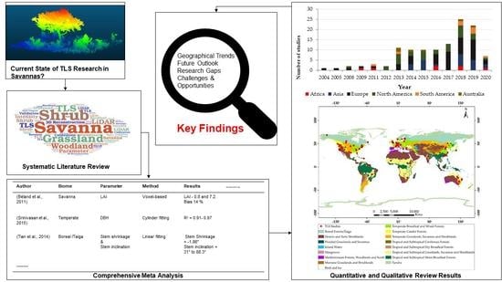
:Savannas are heterogeneous ecosystems, composed of varied spatial combinations and proportions of woody and herbaceous vegetation. Most field-based inventory and remote sensing methods fail to account for the lower stratum vegetation (i.e., shrubs and grasses), and are thus underrepresenting the carbon storage potential of savanna ecosystems. For detailed analyses at the local scale, Terrestrial Laser Scanning (TLS) has proven to be a promising remote sensing technology over the past decade. Accordingly, several review articles already exist on the use of TLS for characterizing 3D vegetation structure. However, a gap exists on the spatial concentrations of TLS studies according to biome for accurate vegetation structure estimation. A comprehensive review was conducted through a meta-analysis of 113 relevant research articles using 18 attributes. The review covered a range of aspects, including the global distribution of TLS studies, parameters retrieved from TLS point clouds and retrieval methods. The review also examined the relationship between the TLS retrieval method and the overall accuracy in parameter extraction. To date, TLS has mainly been used to characterize vegetation in temperate, boreal/taiga and tropical forests, with only little emphasis on savannas. TLS studies in the savanna focused on the extraction of very few vegetation parameters (e.g., DBH and height) and did not consider the shrub contribution to the overall Above Ground Biomass (AGB). Future work should therefore focus on developing new and adjusting existing algorithms for vegetation parameter extraction in the savanna biome, improving predictive AGB models through 3D reconstructions of savanna trees and shrubs as well as quantifying AGB change through the application of multi-temporal TLS. The integration of data from various sources and platforms e.g., TLS with airborne LiDAR is recommended for improved vegetation parameter extraction (including AGB) at larger spatial scales. The review highlights the huge potential of TLS for accurate savanna vegetation extraction by discussing TLS opportunities, challenges and potential future research in the savanna biome.
1. Introduction
1.1. The Role and Importance of Savannas
Savannas are heterogeneous ecosystems characterized by mixed physiognomies of woody and herbaceous layer [1]. Savanna ecosystems span one-fifth of the global land [2,3] which makes up approximately 20% of the terrestrial vegetation and contribute 30% of all terrestrial ecosystem gross primary productivity [4,5]. Savanna ecosystems also contribute significantly to the global carbon cycle with a net primary productivity of 1 to 12 t C ha−1 year−1 and a carbon sequestration rate averaging 0.14 t C ha−1 to 0.39 Gt C year−1 [4].
Savannas are vital biomes that play a major role in the provision of ecosystem services. Moreover, they contribute significantly to the socio-economic needs of most rural households, especially in Africa, where many are dependent on natural resources for their livelihood [6,7]. Savannas support approximately 20% of the world population and account on average 28% of household income in rural areas of developing countries [8,9]. In west and central Africa, income from bushmeat is equivalent to approximately $1000 per year [7].
Since savannas are home to 20% of the world’s population, humans have caused changes in these ecosystems through land clearing for agriculture and livestock production, infrastructure, fire lighting or suppression and fuelwood collection [9,10]. The alteration of savanna structure and function has direct effects on woody vegetation and results in woody encroachment as a result of the interaction of drivers mainly herbivory, fire and atmospheric carbon dioxide [11,12]. Anthropogenic land use and land cover change affects vast areas of the savanna ecosystem and the consequences can be substantial for the regional climate cycle [9]. Against this background, it is important to regularly map and monitor savannas and to quantify the carbon pools and dynamics of these ecosystems because they contribute significantly to global productivity [13].
1.2. Monitoring of Savannas Using Remote Sensing
Much of the current understanding on savanna vegetation structure is derived from traditional field-based methods, such as forest inventories, permanent sample plots and transects [14,15]. Field-based estimates are essential in the validation of remote sensed data [16], though they are limited in that they are time consuming, expensive, labour intensive and often require destructive sampling [17,18]. Remote sensing techniques are more appropriate for monitoring when compared to traditional methods [19]. Especially for consistent analyses at different spatial and temporal scales and when considering inaccessible areas, remote sensing with limited fieldwork has been proposed as an efficient method [17,19].
The main types of Earth observation data used for vegetation studies are based on optical (multispectral, hyperspectral), Radio Detection and Ranging (RADAR) and Light Detection and Ranging (LiDAR) sensors [20].
Multispectral data can be acquired from spaceborne (satellites) or airborne (aircrafts, Unmanned Aerial Vehicles (UAVs) platforms and from the ground imagery (spectrometers). Multispectral data has the advantage of higher spatial resolution [21] and is publicly available for most regions in the world e.g., Landsat data. It is limited in terms of spectral resolution [21] and spaceborne optical data often suffer from cloud cover and mixed pixels [20,22].
Hyperspectral data can be acquired from spaceborne and airborne sensors and hyperspectral cameras [23]. Hyperspectral data is acquired in hundreds of narrow bands, and thus it has a higher spectral resolution enabling distinguishing of vegetation types [24]. It is limited though in terms of spatial resolution [21] and suffers from band redundancy where bands are strongly correlated [24].
RADAR data have the advantage of being largely independent of atmospheric and illumination conditions. However, they are limited because data-specific issues need to be compensated for or at least considered when using RADAR for vegetation monitoring [25]. Among others, these issues comprise the geometry of Synthetic Aperture RADAR (SAR) imagery, the dielectric properties of the surveyed surfaces, RADAR speckle complications due to the separation between signal and noise in the data, RADAR shadow and saturation problems [25].
To date, LiDAR systems are considered to be the most accurate and recommended remote sensing technology for vegetation parameter retrieval by producing high-resolution 3D data called point clouds [26,27]. They are available as space and airborne, mobile and UAV as well as terrestrial LiDAR sensors [27]. Spaceborne LiDAR provides the opportunity to make large-scale assessments of vegetation structure for global to regional biomass estimation [28]. Airborne LiDAR is also able to cover relatively large areas and measures vegetation structure with high accuracy [29]. Both spaceborne and airborne LiDAR systems are limited in detecting smaller trees and shrubs. The latter are key attributes in savanna ecosystems [30]. By using airborne or spaceborne LiDAR these attributes and are restricted to landscape level estimates. Mobile and UAV LiDAR sensors offer a faster approach for acquiring 3D point clouds. However, mobile LiDARs are constrained in extracting canopy and height attributes [31], whereas UAV LiDARs have difficulties in capturing tree trunks [32] and are also limited in flight time due to batteries [33]. An overview of the main advantages and disadvantages of the described monitoring technologies i.e., (field surveys, multi-spectral, hyperspectral, RADAR and LiDAR) platforms are also discussed in Béland et al. [27], Eisfelder et al. [34] and Galidaki et al. [35].
1.3. Terrestrial Laser Scanning (TLS)
Terrestrial Laser Scanning (TLS) has grown in interest because of its ability to produce 3D point cloud data for characterizing vegetation structure [36]. Accordingly, over the past decade, a considerable amount of research has been directed towards the 3D quantification of vegetation structure using TLS [37,38]. Vegetation structural parameters are difficult and laborious to measure in the field, especially in complex ecosystems like the savanna. However, TLS has proven efficient in deriving these parameters because it produces consistent and objective measurements with high precision. Furthermore, TLS measurements are relatively easy to interpret and parameter extraction can be automated [39,40].
A terrestrial laser scanner or ground-based LiDAR is a LiDAR system from which detailed 3D information called point clouds can be collected [41]. Using a laser beam, terrestrial laser scanners provide a high-resolution 3D view of the objects [36]. Depending on their range measurement principle, terrestrial laser scanners are classified into two types: phase shift or time of flight scanners [36,42]. Phase shift scanners measure distances by analysing the shift between the emitted and the received laser wave. In contrast, time of flight scanners compute distances based on the difference between the emission and reception of the laser pulse [42].
TLS measurements can be collected based on single or multiple scans. Using single scans, the scanner is placed at a single location within the study area whilst multiple scans are obtained when the scanner is placed at several positions within the test site [43]. For rapid and efficient extraction of vegetation parameters with reduced fieldwork and faster post-processing, single scans are preferred [44]. However, this approach is prone to occlusions (e.g., a tree being in the scan shadow of another tree or any other object) reducing the accuracy of vegetation structure retrieval and the ability to get a full 3D representation of an object [44]. For the best plot coverage and a complete 3D description of the objects under consideration, a multi-scan TLS setup is necessary [31,36].
Multi-scan TLS data allow for reliably retrieving common tree attributes such as Diameter at Breast Height (DBH), tree height, canopy structure and vertical height profiles [45,46]. In addition to these parameters, more detailed and complex vegetation attributes such as leaf water content [47], basal area and stem density [48], Above Ground Biomass (AGB) change [49], tree crown change [50] stem curve profiles [51], stem shrinkage [52], have been derived from TLS point clouds.
TLS provides unmatched 3D information on vegetation structure right down to branch and leaf scales, making it far superior to data obtained through traditional field work [38,53]. Using the intensity of the returned laser pulses, TLS can be used to map pigment concentration, photosynthetic capacity and water content of the vegetation [27]. It is also possible to separate wood from leaf material [54,55]. TLS offers a non-destructive approach to quantify canopy and stem volume with high accuracies, thereby enabling the estimation of AGB with reduced uncertainties as well as the development and improvement of reliable allometric equations [56,57]. TLS also enables the estimation of individual tree components [58] and it can also be employed as a calibration and validation dataset because of its ability to acquire data from the ground that is similar to traditional measures of vegetation structure [59,60].
The inherent heterogeneity of savannas presents a challenge regarding accurate vegetation characterization. To overcome this challenge, 3D data on the horizontal and vertical structure of the savanna are needed. TLS is able to account for savanna heterogeneity (Figure 1) by providing detailed information on all savanna vegetation types and layers [61,62]. It therefore holds much potential for making holistic AGB assessments, including long and short stature vegetation [63,64,65].
Different drivers can result in the loss of large trees in the savanna landscape [66] and changes in vegetation structure. The non-destructive nature of TLS makes it more so suitable for quantification of change in vegetation structure and reduction of uncertainties when estimating AGB [50,67]. The use of repeated TLS scans allows for monitoring these and other losses (and potentially gains) in savanna AGB over time. Multi-temporal TLS therefore holds the potential to support carbon accounting programmes such as REDD+.
While TLS is able to capture the 3D configuration of vegetation at high spatial resolution, data can only be acquired for a limited areal extent and data acquisition usually requires extensive field work [68]. This problem is solved by the integration of TLS with other remote sensing data to ensure the coverage at landscape scales. For example, landscape studies were conducted in the savanna by the integration of TLS with airborne LiDAR [69], TLS with MODIS satellite data [70] and TLS with ALOS PALSAR L band data [62]. Moreover, TLS scans frequently feature occlusions (“shadows”) caused by objects close to the scanner which, in turn, block the view of other objects further away. Although occlusions are not a major problem in open savannas, they can be minimized by the use of multiple TLS scans [30,64]. Another shortcoming of TLS systems is that the point density decreases with distance from the scanner, an effect called beam divergence [68,71] which causes the point cloud to be unreliable at a certain distance.
1.4. Overall Goal and Objectives of the Review
This paper aims to review the scientific literature on the use of TLS for vegetation analyses. It puts a special but not exclusive geographic focus on savannas in order to establish the current status quo in savanna vegetation parameter extraction. In contrast to existing reviews in the TLS literature [72,73], this study presents the current TLS methods in practice and identifies those suitable for accurate biomass assessments in the savanna biome. To address this gap, our meta-analysis takes a detailed look at the geographic distribution of TLS studies, the parameters retrieved from TLS point clouds, known retrieval methods as well as the main opportunities and challenges arising from the studied literature. The remainder of the paper is structured as follows: Section 2 presents the approach and Section 3 the main findings of the review. The main discussion points and conclusions derived from the review are presented in Section 4 and Section 5, respectively.
2. Materials and Methods
A systematic literature review was conducted in Web of Science [74]. Access to its catalogue was granted through the Thüringer Universitäts- und Landesbibliothek Jena (ThULB). The advanced search functionality in Web of Science was used to develop and apply a set of predefined queries. The search included all journals in the Web of Science Core Collection™ database. Peer-reviewed conference papers were also included. Searching for keywords in the title (TI) and in some instances in all fields (ALL) (when a query returned fewer than ten articles) was performed with a time frame up to May 2020. The time span for the search was all years that is from 1945 to 2020. In the event that a search query returned more than 100 articles, the search was refined by the research areas forestry or remote sensing to narrow down on specific studies employing TLS for vegetation parameter extraction. Each query consisted of different keywords and related synonyms (Table 1) which were combined through logical operators (i.e., “AND”, “OR”).
An example of one of the search queries developed is: TI = ((TLS OR Terrestrial LiDAR OR Terrestrial Laser Scann *) AND (Tree Structur *)). This search query would return all journal articles that have either the word or terrestrial LiDAR or terrestrial laser scanner or terrestrial laser scanning and the word tree structure or tree structural in their title.
Following the above search scheme, a total of 158 research articles were initially retrieved from Web of Science. In a second step, certain papers were retained for the review according to a prescribed set of criteria. The criteria used to refine the initial search results were as follows:
- ⮚
- The study under consideration focused on the extraction of one or more vegetation parameters from TLS point clouds. For example, a study was only considered if parameters like the DBH or AGB were derived on the basis of TLS point clouds [75];
- ⮚
- ⮚
- The study under consideration reviewed TLS as a remote sensing technology [39];
- ⮚
This resulted in a final number of 113 reviewed publications. To qualitatively and quantitatively assess the final selection of papers, a comprehensive meta-analysis was conducted based on 18 predefined study attributes. Besides author(s), year of publication and publishing journal, the list of reviewed meta-parameters included: study area(s) (country, continent, biome); type of laser scanner used (TLS model/device); range finder of the scanner (phase shift or time of flight); type of TLS data used (xyz and intensity); scanner setup (TLS settings for scanning); field setup (use of reflectors, GPS/dGNSS); number of scans (single vs. multiple scans); parameters retrieved (e.g., DBH, vegetation height, crown diameter); retrieval method (algorithm used); number of studied trees and shrubs (total number of trees/shrubs measured in the research); performance metrics such as coefficient of determination (R2), Root Mean Square Error (RMSE) and bias; main discussion points (e.g., advantages and limitations of a used approach); and lastly research gaps and potential avenues for future research. The above search efforts were undertaken to ensure that all relevant TLS literature was collected. The full list of papers considered and finally selected in this review is available in Table S1 (supplementary material).
3. Results
3.1. General Overview
Of the 113 publications used for the detailed review, 80% of the publications focused on the extraction of vegetation parameters from TLS point clouds, 12% used TLS as auxiliary data (e.g., TLS data used to validate airborne LiDAR) [78,79,80] and 8% applied TLS for technical experiments (e.g., reflectance modelling using TLS intensity data) [81,82,83]. Among the 113 papers, 97 were publications from peer-reviewed journals whilst 16 were peer-reviewed proceedings. The most popular journals were Remote Sensing (20 studies), Remote Sensing of Environment (9 studies), Agricultural and Forest Meteorology (8 studies) and ISPRS Journal of Photogrammetry and Remote Sensing (6 studies). Most proceedings papers stem from the International Geoscience and Remote Sensing Symposium (IGARSS), with 9 studies.
3.2. Temporal and Spatial Patterns
Figure 2 shows the trend observed in the number of TLS studies. Beginning in the early 2000s, TLS technology evolved slowly. New systems with a range of capabilities and applications emerged and this explains the rise in the number of studies from the early 2000s to date. TLS technology had a real breakthrough in vegetation studies around 2013 and the upward trend seems to continue in 2019. A further significant increase in peer-reviewed studies can be observed for 2018 and 2019 (25 and 22 articles, respectively). During this time, the number of published papers per year has more than doubled when compared to the period after the breakthrough (on average 10.8 studies per year for 2013–2017).
The geographic distribution of the reviewed studies by country is shown in Figure 3. To date, most studies were conducted in the United States, China and Finland. From a continental perspective, Europe has the highest number of studies (38%) [84,85,86] followed by North America (24%) [46,59,87] and Asia (19%) [88,89,90]. Africa (6%), Australia (5%) and South America (7%), with more than half of their landmass belonging to the savanna biome [1,2], had few TLS studies [64,91,92].
The geographic distribution of studies by biome (after Olson et al. [93]) and the percentage of reviewed studies per biome are shown in Figure 3 and Figure 4. Studies that were conducted in more than one biome were counted multiple times and four laboratory studies were excluded from this analysis, resulting in a sample size of n = 114. The reviewed papers covered a total of 11 biomes. While most studies were conducted in temperate forests (47%) [75,94,95], much less papers were published in boreal (16%) [96,97,98], tropical and subtropical forests (10%) [99,100,101] as well as grasslands and savannas (9%) [70,91,92]. The cumulative total for the savanna biome was 13%, including 4% of savanna research conducted in temperate regions (“Temperate Grasslands Savannas and Shrubland”).
3.3. TLS Instruments and Data Used
A variety of TLS instruments can be purchased nowadays. They are offered by different manufacturers, with the main companies being RIEGL Laser Measurement Systems GmbH [102], FARO Technologies Inc [103] and Leica Geosystems [104]. Among others, TLS instruments differ in their, measurement range (the maximum distance that can be scanned e.g., 600 m), sample rate (pulses per second e.g., 122,000), wavelength (e.g. 1550 nm (near-infrared)), angular sampling (angle measurement resolution e.g., 0.02°), waveform (discrete or full-waveform), range measurement principle (time of flight or phase shift), size, mass and power efficiency. Based on our review, Table 2 provides an overview of frequently used TLS instrument models. Among the most popular scanners were Riegl VZ 400 (26 studies) [90,105,106], Leica HDS6100 (10 studies) [107,108,109], Riegl VZ 1000 (9 studies) [110,111,112], Faro Focus 3D (7 studies) [50,67,113] and Faro Focus 3D X 330 (also 7 studies) [83,114,115].
Figure 5 shows the number of scan positions and the area covered in the reviewed studies. It becomes clear that a larger area requires a higher number of scan positions, the higher the number of scan positions the fewer the studies and most studies use up to 10 scan positions and cover an area of less 5000 m2. The number of scan positions and area covered also depend on the vegetation type and the level of detail required for the specific research. For high detail data, some studies employed a high number of scan positions on a relatively small area. Li et al. [63] used 18 scan positions on a 400 m2 plot on shrubs and Lau et al. [99] used 16 scan positions on each selected tree in a 1200 m2 plot in a tropical forest. Most inventories follow a field setup with multiple scans, with five (28 studies) [121,122,123], four (23 studies) [124,125,126] and three (13 studies) [113,127,128] scan positions being the most popular. However, a single scan experimental design is also very common (28 studies [83,89,129]).
TLS instruments provide two types of data that can be used for forestry and vegetation studies. These are 3D coordinates (XYZ data, point clouds) and the intensity of the reflected signal. The signal can either be discrete or full-waveform. Discrete data provide single or multiple returns for each laser pulse [76,130]. Full -waveform contain measurement of the reflected laser beam as a function of range [76,130]. These two data types can be integrated with auxiliary data from the field, including RGB images from digital cameras. Most studies used XYZ data (85 studies) [131,132,133] whereas intensity information was considered much less (8 studies) [129,134,135]. A triple combination of both data types and RGB images (2 studies) [121,136] as well as a combination of XYZ and RGB (3 studies) [75,111,137] was not commonly observed. Instead, a number of studies took advantage of XYZ and intensity data (15 studies) [127,138,139]. No paper presented results based on a combination of TLS intensity data and RGB images.
3.4. TLS Point Cloud Pre-Processing
The scanner in use usually comes with software for pre-processing the point cloud; for example, Riegl scanners come with Riscan Pro, Faro with FARO Scene and Leica with Leica Cyclone. The first stage in prepossessing if a multi scan setup was used is to conduct coarse registration and georeferencing to the local coordinate system using the retroreflectors as tie points [43,96]. Fine registration can also be achieved using multi-station adjustment through an iterative closest point algorithm in Riscan Pro software [43,140]. Multi-station adjustment requires a minimum of 3 TLS setups with a minimum overlap of 30%. The algorithm uses surface and point normals to compute the adjustment [141]. The registered point cloud is then clipped to the radius of the plot in the case of circular plots or to the extent of the plots or to remove low density points at the plot edges [140,142].
The final pre-processing stage involves filtering the point cloud to remove noise from the data [43,121,142]. Noise and outlier removal is done to increase accuracy and reduce errors when extracting information from the point cloud data [115]. The noise can be classified into internal and external noise, internal noise being the inherent noise from the scanning device and external noise from the reflective nature of the scene [143,144]. The common noise points from vegetation are leaves, extremely high or low points, and from occlusions [115,144]. The filtering is performed using various approaches such as statistical, neighbourhood, projection, signal and partial differential based filtering techniques [144]. For example, in the case of statistical outlier removal, the filtering reduces the error on the point cloud by computing the average distance to its neighbours and rejects points that are further away from the average distance [115,144]. Point cloud filtering can be performed in software packages such as Cloud Compare, LAStools, MeshLab and programming libraries such as Point Cloud and Open Graphics Library [143]. After pre-processing various algorithms are then applied to extract the vegetation parameters.
3.5. Methods Used with TLS Point Clouds
Of the 113 papers reviewed, 87 papers focused on the extraction of vegetation parameters from TLS point clouds. Of the 87, only 15 studies worked in the savanna biome [39,145,146]. The most frequently employed methods to derive vegetation attributes are the RANdom SAmple Consensus (RANSAC) algorithm for extracting DBH, stem curve profiles and the detection of stems [97,147], the use of the highest z coordinate of the point cloud for estimating heights [61,148], voxel-based and radiative transfer models for assessing LAI [149,150], Canopy Height Models (CHMs) for delineating crown attributes [91,92], and Quantitative Structure Models (QSMs) for computing tree volume and branch parameters [151,152]. Popular software packages to implement and work with these methods are Lastools [153], Matlab [154], R [155] and Python Programming [156], Cyclone [157], FARO Scene [158], RiscanPro [159], CompuTree [160] and Cloud Compare [161]. For evaluating the above extraction techniques, performance metrics such as R2, RMSE and bias are typically used [51].
3.6. Vegetation Parameters Extracted from TLS Data
The vegetation parameters that can be retrieved from TLS data can be broadly classified into primary and secondary parameters [22]. Primary parameters are those directly derived from the TLS point cloud, such as DBH, height, volume and tree canopy characteristics [22]. Secondary parameters can only be estimated indirectly and are derivatives of primary parameters. They are usually obtained through modelling [22]. Examples of secondary parameters are AGB, basal area, stem density and LAI [22]. Besides the common vegetation parameters e.g., DBH and height, some studies focused on extracting unique and complex vegetation parameters such as tree planar projection [162], the elevation of angle and azimuth of stem inclination [52], clumping index [163], ground cover [92] and structural loss [164].As shown in Figure 6, most of the reviewed studies retrieved primary parameters, including DBH (41), height (32), tree canopy features (e.g., crown diameter, canopy cover) (20), trees or tree stems (20) and tree volume (15). With only five and six articles, respectively, branch parameters and stem curve profiles gained the least attention. Of the secondary parameters, LAI was the most extracted parameter (21), followed by AGB (11), basal area (5) and stem density (3). Details regarding specific parameters and the methods to retrieve them are provided in the following subsections. Particular emphasis is put on savanna ecosystems.
3.7. Primary Vegetation Attributes
3.7.1. DBH
From the reviewed papers, only one study derived DBH in the savanna [92]. Muir et al. [92] employed circle fitting to single-scan TLS data at heights between 1.28 m and 1.32 m above the Digital Elevation Model (DEM) in an open woodland site in Central Western Queensland Australia. They compared the resulting stem diameter measurements with data collected in the field and obtained an R2 value of 0.77 [92]. Slightly better performances are often observed for DBH extraction in temperate, tropical and boreal forests, with R2 values ranging from 0.81 to 0.99 [94,165,166] when compared to field reference data. For a pine woodland test site in France, least-squares circle fitting was reported to be the most accurate method (RMSE = 0.019 m) for estimating DBH when compared to least squares cylinder fitting and circular Hough transformation [85]. Similarly, Calders et al. [40] and Chen et al. [167] obtained R2 values of 0.97 when using least squares circle fitting for DBH estimation with a multi-scan TLS scan with 5 positions in a eucalypt open forest and boreal forest respectively. Yurtseven et al. [148] obtained an R2 value of 0.99 with a multi-scan with 8 positions in a Mediterranean forest employing randomised hough transformation with least square regression. In general, multiple TLS scans and a lower stem density yielded the best results [114,168,169].
3.7.2. Vegetation Height
Tree height estimation in the savanna was reported in five studies [30,62,91,92,145]. Odipo et al. [62] and Muir et al. [92] employed the use of CHMs to estimate tree height from multiple and single TLS scans (30 positions and single scan) and obtained R2 values of 0.64 and 0.98 respectively when compared to ground referenced data. Singh et al. [30] observed an RMSE of 0.25 to 1.45 m based on multi-scan Long Range -TLS (LR-TLS) with 4 positions. They computed heights by measuring the vertical distance between treetops and the stem base. Kirton et al. [145] employed cylinder fitting to extract tree height and obtained a standard error of ±0.002 m using a TLS single scan. It was observed in this study that it is more challenging to derive the height of savanna shrubs than it is for savanna trees. Muir et al. [92] also reported that shrub heights are difficult to calculate from TLS data, with R2 values of 0.381 and 0.08 for maximum and average shrub height, respectively. In contrast to this observation, the extraction of height from short stature vegetation was achieved with reasonable accuracy in montane areas as well as desert and xeric shrubland biomes [170]. Vrlingie et al. [170] applied a 2-D spatial wavelet analysis on a TLS derived CHM to extract shrub height and achieved an R2 of 0.94 when compared to field measured shrub height.
3.7.3. Stem Detection
The detection of stems from TLS point clouds is an important first step in processing, to enable extraction of other vegetation parameters [171]. Only one study [147] from the review was conducted in the savanna biome. Burt et al. [147] employed treeseg algorithm (which extracts tree point clouds from larger point clouds) on a tropical and on an open vegetation cloud using TLS multi scans with 5 positions. They achieved 70% and 96% stem detection accuracy, respectively [147]. The detection of stems was achieved with high accuracies in temperate and boreal forests [138,171]. Kelbe et al. [138] used voxel stem segment modelling on a single TLS scan dataset acquired using low resolution TLS in various forest types in New England. Stems were detected with accuracies of (R2 = 0.99; RMSE = 0.16 m) [138]. In a boreal forest Zhang et al. [171] employed connected component segmentation using both single and multi- scan with 5 positions. They achieved stem detection accuracies of 93% for single scan and 99% for multi-scan TLS setup when compared to reference data [171]. To date, most of the commonly used algorithms (e.g., density-based clustering [172], Hough transformation [85] and RANSAC cylinder fitting [48,173] used for stem detection achieved stem detection accuracies of 70% to 99% when applied in temperate, tropical and boreal forests.
3.7.4. Crown Attributes
Among the tree crown attributes dealt with in the scientific literature are canopy cover, canopy height/length, crown width/diameter and tree crown change. In the savanna biome, extraction accuracies for trees were better as compared to shrubs. Singh et al. [30], Odipo et al. [62] and Muir et al. [92] employed CHMs to determine canopy cover. Singh et al. [30] achieved an RMSE of 5.7–15.9% at distances up to 500 m with 4 scan positions, whilst Odipo et al. [62] and Muir et al. [92] achieved R2 of 0.56 and 0.93 as compared to the ground referenced data with 30 and single scan positions respectively. Lower accuracies were obtained when estimating shrub canopy cover, with Muir et al. [92] reporting an R2 of 0.23 when compared to field measurements. Yet, the application of 2D spatial wavelet analysis achieved an R2 of 0.51 for 36 shrubs in a desert and xeric shrubland environment [170]. In this study, shrub crown area was calculated using spatial wavelet analysis using the detected radius while the actual shrub crown area was determined by measuring the minor and major axis and then calculating the crown as an ellipse [170]. The use of different algorithms for accurate extraction of canopy cover was also investigated by Yurtseven et al. [148] in a mediterranean woodland and scrub. They employed convex and concave hulls and they concluded that the concave planar underestimates canopy cover area as compared to the convex hull. A method to quantify canopy cover change was considered by Olivier et al. [50] in a sugar maple and balsam fir forest in Canada. They used bi-temporal multi-scan TLS data to identify vegetation boundaries, extract new material formed or displaced between the two-time period [56].
3.7.5. Tree Volume and Branch Parameters
Volume of standing trees or above ground volume is total stem wood and branches [174]. Branch parameters are parameters like branch total length, branch diameter, branch insertion angle, branch depth into the crown and branch radius. Over the years, a range of algorithms has been developed to compute tree volume and branch parameters from TLS point clouds [151,175]. However, none of the corresponding studies was conducted in the savanna biome. QSMs are the most common algorithms used in literature [96,151,175]. They have the ability to provide reliable volumes estimates of stem and branches of trees, but also have limitations in reconstructing leaves [176]. Figure 7 shows an example of a 3D point cloud and the resulting QSM. Branching structure and branch lengths were determined in boreal and tropical forests using QSM [151,175]. Kaasalainen et al. [175] used a multi scan with 2 positions to reconstruct branching structure and concluded that branching structure can be reproduced with ±10% accuracy when compared to laboratory reference measurements. Lau et al. [151] used a multi-scan with 13 positions and successfully reconstructed 87% of the branch lengths. They compared the reconstructed branch lengths to manually measured branches from destructively harvested trees [151]. For the estimation of shrub total and green biomass, Olsoy et.al [54] employed voxel-based and 3D convex hull algorithms to first determine shrub volume in a xeric sagebrush ecosystem in Southern Idaho, USA using multi scan with 2 positions. They then modelled shrub total and green biomass by subsetting the point cloud into green and non-green woody components based on the difference in their reflectivity. Their findings showed that convex hull algorithms (R2 = 0.92, R2 = 0.83) performed slightly better than the voxel-based method (R2 = 0.86, R2 = 0.73) in estimating total and green biomass respectively [54]. The TLS derived shrub biomass was compared to the destructive samples of shrubs [54]. These and other volume-related algorithms (e.g., bounding cuboids, outer hull models, square-based columns) have also been compared for test sites in the temperate and tropical regions [101]. It was found that convex hull techniques tend to overestimate while the square-based column method underestimates volume. Moreover, voxel-based estimates are mainly affected by the point density and level of occlusions in the point cloud [101].
3.7.6. Stem Curve Profiles
Stem profiles or stem taper is the “stem diameter measured as a function of height” [179]; that is, how the diameter of the tree changes at different heights along the stem. Six studies used TLS point clouds to determine stem curve profiles, five of the studies were conducted in boreal forests [48,51,52,162,166] and one was conducted in temperate broadleaf and mixed forest [58]. The methods used to extract stem curve profiles from TLS point clouds are either circle or cylinder fitting at different height bins [48,51,52,58,162,166]. Maas et al. [58] extracted stem curve profiles using circle fitting at multiple heights and obtained an RMSE of 4.7 cm when compared to a harvested stem. Liang et al. [51] observed that most algorithms used for the extraction of stem curve profiles results in an RMSE of 1.3 and 6.0 cm for single scan data and 0.9 and 5.0 cm from multi scan data for three different stem densities (i.e. low, medium and high stem densities) in a boreal forest. The RMSE values obtained are a function of both the stem density and the number of scan positions employed [51].
3.8. Secondary Vegetation Attributes
3.8.1. AGB
AGB is defined as “the total amount of biological material (oven-dried) present above the surface in an area” [180]. AGB is the most important secondary attribute derived from TLS point clouds. The accurate extraction of all other parameters is a necessity in improving tree biomass estimation. A total of five studies estimated AGB in the savanna using TLS [62,64,70,90,126]. Zimbres et al. [64] predicted plot AGB of three vegetation types in the Brazilian cerrado. The TLS derived AGB was validated against the AGB values obtained from allometric equations. The R2 values obtained were 0.92 and 0.88 for the woodland savanna dry and rainy season respectively and 0.58 for the forested savanna. Due to occlusions, no conclusive results were obtained for the gallery forest [70]. Cuni-Sanchez et al. [70] estimated AGB change in five different vegetation types using vertical plant profiles extracted from a multi-scan TLS over a period of 20 years in Gabon. However, the savanna plots were not assessed because all the trees had a diameter of less than 10 cm [70]. Odipo et al. [62] also estimated AGB change in a south african savanna using TLS derived canopy cover and height metrics for plot level AGB and then further extrapolating to a wider scale using multi-temporal L band SAR. The TLS derived metrics were validated with field measured parameters. Significant relationships were obtained between the TLS derived predictors (canopy cover & height) with field biomass (R2 = 0.93). Seven variables extracted from TLS data were used to build regression models with field measured AGB to estimate grass biomass in China [90]. The regression methods used were Simple Regression (SR, Stepwise Multiple Regression (SMR), Random Forest (RF) and Artificial Neural Network (ANN). Results obtained showed that the highest prediction of biomass was obtained using SMR model (R2 = 0.84), followed by SR (R2 = 0.80), RF (R2 = 0.78) and lastly ANN (R2 = 0.73) [90]. Cooper et al. [126] investigated the application of Structure from Motion (SfM) photogrammetry and TLS for the estimation of grass biomass and compared this to destructive harvest grass biomass. The R2 values for the TLS derived grass biomass was 0.46 and total biomass was 0.57, whilst for the SfM it was 0.54 for the grass biomass and 0.72 for the total biomass [126]. TLS data have also been used to derive tree and grass AGB change [49,115]. Srinivasan et al. [49] extracted various tree parameters (including AGB) from loblolly pines in Texas, USA by the use of multi-temporal TLS data. The best results (R2 = 0.50, RMSE = 10.09 kg) were obtained by directly estimating AGB change from the point cloud when compared to field measured AGB change. Guimarães-Steinicke et al. [115] also investigated grass biomass temporal change in Thuringia, Germany. They used 25 TLS derived metrics to model biomass [115].
While most of the reviewed studies focused on the estimation of tree biomass, only few papers dealt with shrub biomass. Shrub biomass was investigated by Greaves et al. [59] in the arctic tundra. They employed a leave one out cross-validation technique of the canopy volume against the harvested shrub biomass to establish predictive relationships between the TLS canopy volume and harvested shrub biomass and between Airborne Laser Scanning (ALS) canopy volume and TLS derived shrub biomass estimates. The TLS produced more accurate predictions of shrub biomass as compared to the ALS (TLS R2 = 0.78 and ALS R2 = 0.62). Li et al. [181] merged TLS and ALS to estimate the biomass of sagebrush in southwest Idaho, USA by building predictive models. TLS derived biomass was used for calibration of a biomass predictive model with an R2 of 0.87. The TLS derived shrub volume was compared to the destructive shrub biomass measurements (R2 = 0.88) [181].
3.8.2. LAI
LAI is defined “as the ratio of leaf area to per unit ground surface area” [39,130]. A study was conducted in the savanna biome by Béland et al. [39]. They applied a voxel-based approach making use of the contact frequency method on six trees. To this end, they employed two multi-scan setups with 2 and 3 positions and compared the TLS derived estimates against direct measurements obtained from leaf harvesting. The leaf area ranged from 30 to 530 m2 whilst crown LAI was 0.8 and 7.2 with a general bias of 14%. To ensure an accurate extraction of LAI, the green and non-green components were distinguished in the TLS data based on a separation threshold applied to the return intensities [39]. Olsoy et al. [182] estimated the LAI of sagebrush from TLS data with 2 scan positions and found that the estimated LAI was highly correlated with their reference field data (R2 = 0.78).
3.8.3. Basal Area
Basal area is defined as a “cross-sectional area of all stems in a plot measured at breast height and usually expressed per unit of the land” [183]. Five studies estimated basal area from TLS point clouds, with four being conducted in a temperate broadleaf and mixed forest [75,78,85,184] and one from the boreal zone [48]. No study has been published yet for the savanna biome. Yrttimaa et al. [48] and Tansey et al. [85] derived basal area from TLS point clouds by first calculation basal area for a single stem, then scaling it to one hectare. The TLS derived basal area was compared to the field derived basal area which was derived by considering the cross-sectional area of a tree to be circular [48]. The R2 observed were 0.87, 0.86 and 0.63 for a plot radius of 6, 11 and 16 m respectively [48]. Côté et al. [184] used an architectural model called LiDAR to Tree Architecture (L-Architect) by reconstructing forest stands with scans of individual trees. The L-Architect derived basal area was compared to the measured values of basal area to assess accuracy. A relative difference of −0.01% was obtained between the L-Architect and field measured basal area [184]. A methodology based on voxel data structure was applied to derive the basal area of individual trees in a heterogeneous vegetation structure in Washington Park Arboretum [75]. The TLS derived basal area was derived by fitting a 3D cylinder primitive to the trunk assuming that the trunk was a geometric circle. The TLS derived basal area was compared to the manually measured basal area. The TLS derived basal area was underestimated compared to the field-based methods for conifers, deciduous and mixed stands (Conifer: Field = 12.3116 m2, TLS = 6.9217 m2; Deciduous: Field = 1.4275 m2, TLS = 1.0172 m2 & Mixed: Field = 1.8431 m2, TLS = 1.575 m2) [75]. Aijazi et al. [78] used a super voxel segmentation method to estimate basal area and concluded that parameter estimation error ranged from 1.6 to 9% from TLS point clouds.
3.8.4. Stem Density
Stem density is defined as “the number of trees per hectare” [185]. Three of the reviewed studies estimated stem density, with one being performed in a savanna ecosystem [92]. Stem density is derived from the number of stems identified in the scanned area and comparing it to the field derived stem density [48,85,92]. Yrttimaa et al. [48] varied the plot size in order to investigate its effects on stem density. The smaller the plot size, the higher the correlation of the TLS-derived stem density with field measurements (r = 6 m | R2 = 0.77; r = 11 m | R2 = 0.67; r = 16 m | R2 = 0.38). Muir et al. [92] determined stem density from TLS point clouds as well. They achieved an R2 of 0.1 and reported a large RMSE of 130.9 trees/hectare that was attributed to plot complexity.
4. Discussion
4.1. Geographical Trends in the TLS Literature
From a global perspective, most TLS studies have been conducted in Europe, North America and China (Figure 3). Despite their large geographical extent in Africa, South America and Australia, savannas have rarely been investigated in these areas. In the early 2000s, TLS-based vegetation studies were mainly conducted in Europe and North America (Figure 2). From 2009 onwards, TLS studies expanded into the rest of the world, including Africa, Asia, Australia and South America. An increasing collaboration among TLS research groups from different parts of the world can explain this observation [57,100,147,171]. To further advance TLS research in savannas and to learn more about their ecology, building scientific capacity in financially constrained countries is key.
Savannas cover ca. 50% of Africa’s landmass. Yet, only 6% of the reviewed studies were conducted in Africa. Of those studies, the majority focused on South Africa. Only a few articles presented results for other African countries, including Mali [39], Ethiopia [186] and Gabon [70]. One reason for this observation is that TLS research in Africa is mainly constrained by financial limitations. The acquisition and processing of TLS data usually require expensive equipment and software [22]. Moreover, it necessitates trained personnel, which is limited in most third-world countries [176]. With the advent of low-cost terrestrial laser scanners [65,187,188], more TLS research can be expected in the future for Africa.
Since savannas cover large geographical areas, TLS data can usually not be used by itself to study an entire region due to its limited footprint. Instead, an integration of TLS point clouds with other geospatial data is necessary for large-scale assessments. In the past, the creation of wall to wall maps of savannas has been achieved by combining TLS with L-band SAR [62] and airborne LiDAR [69]. Currently, the existence of freely available satellite data from Sentinel-1/2 and Landsat 5–8, as well as coarser resolution imagery from MODIS [70] can resolve upscaling issues from fine spatial resolution from TLS to medium resolution from Landsat and Sentinel then to coarse resolution using MODIS. The planned launch of BIOMASS by the European space agency and Multi-footprint Observation LiDAR and Imager (MOLI) by JAXA after Global Ecosystems Dynamics Investigation (GEDI) and Ice Cloud & Elevation Satellite-2 (ICESat-2) will present an opportunity for landscape-level studies of the savanna [60]. Based on these and similar data sets, TLS point clouds can be used in wide-area mapping for calibration and validation purposes [60].
4.2. Challenges & Opportunities
Single and multiple scans (five, four, three and two positions) were found to be the most commonly used TLS setups in the reviewed literature. Single scan approaches have been used successfully to estimate DBH [138,166], height [92] and to detect stems [189]. Single scan inventories received a lot of attention because they allow for fast and less labour intensive data acquisitions and do not require the registration of multiple point clouds [109,112]. However, single scan approaches are also more prone to occlusions [43]. Data from multi-scan TLS campaigns were shown to yield higher accuracies and reduced error margins [45,139]. Therefore, multiple TLS scans with larger plot sizes (>15 m in radius) provide the only opportunity to adequately capture the heterogeneous nature of savannas and to characterize the full spectrum of savanna vegetation structure [92]. Depending on the parameters to be extracted, the requirements to be met and the available resources, the choice between a single- or multi-scan TLS setup should be made carefully. For example, long range single scans give reliable data in the dry season (leaf-off) and not in the wet season (leaf-on) [30].
DBH is one of the most reliable proxies for biomass [190]. This is why it is also the most frequently measured quantity not only by foresters, but also with regard to the reviewed literature. It has been shown that DBH can be delineated automatically based on multiple TLS scans [40]. However, these techniques have not yet been adjusted or tested for more complex vegetation structures [88]. To date, most algorithms to retrieve DBH (and also stems and stem curve profiles) assume a circular or cylindrical stem geometry. However, these rather simple geometries are not well-suited to describe the short stature vegetation and deformed trees that are typically found in savannas [40,191]. While a number of DBH extraction techniques (e.g., RANSAC algorithm [186], point cloud slicing at 1.3 m [75], least-squares circle fitting [52] and Hough transformation [86] exist), they have only been developed and demonstrated in temperate and boreal forests. For savannas, only the circle fitting method has been explored yet [92].
Height was extracted from TLS point clouds in the savanna, mostly through the employment of CHMs to achieve the goal. Muir et al. [92] obtained an R2 of 0.97 and 0.38 for TLS-based estimates of tree and shrub heights, respectively. Small stature woody vegetation is often not well captured by CHMs, which leads to an underestimation of its height when interpolation is used to create the canopy surface [170]. This issue has not yet been adequately addressed, and more accurate height assessment techniques still need to be developed [170]. Potential ways to achieve this would be to elevate the scanner above the vegetation layer or place the scanner on a suitable vantage position [30,92], to capture TLS data of shrubs with higher point density (e.g., 16 pts per m2, [170]) and to distinguish between trees and shrubs in the TLS point cloud and to create two corresponding tree- and shrub-related CHMs that can be analysed separately [92].
Other methods for vegetation height extraction are available, including the combined analysis of TLS and airborne (also UAV) LiDAR data [140,192], the highest z-coordinate (height is derived by the highest value of the return) [51], the vertical distance between the highest point and stem base at the ground (the vertical distance is measured from the base of the stem to the highest point on a segmented point cloud) [30] and cylinder fitting (a cylinder is fitted on a segmented point cloud and the height is denoted as the highest point in a vertical cylinder) [58,145]. While they are also not without errors, these techniques have neither been developed, adjusted nor evaluated for savannas. Known problems, e.g., uncertainties from treetop shading [86], are especially common in the riparian zones of savanna ecosystems.
The extraction of LAI using TLS point clouds is not very common across all biomes [22] including the savanna. Calders et al. [79] argue that caution is needed when using LAI estimates and the variable that is measured from ground-based sensors is effective Plant Area Index (ePAI) and effective Wood Area Index (eWAI). They recommend that TLS measurements are ideal for estimation of gap fraction, ePAI and eWAI as compared to instruments that are dependent on certain illumination conditions [79]. Gap fraction is an indirect way of estimating LAI and TLS is recommended for the estimation of gap fraction to derive ePAI and eWAI [79]. It has been used successfully in the past to estimate LAI [193]. TLS intensity data can also be used to compute LAI. They allow for differentiating between photosynthetically active (green) from non-active (woody) vegetation parts [39,54]. However, they can also be compromised by instrumental, atmospheric and object properties as well as the scanning geometry [82,129]. In order to reliably make use of TLS intensity data for vegetation applications, conversion of instrumental intensity into the proportional or equal target reflectance is required [129,135].
While tree crown attributes have been successfully derived from TLS point clouds, more research needs to be directed towards crown change and shrub parameters. With regard to the former, the method by Olivier et al. [50] needs to be tested in the savanna biome. Vierling et al. [170] suggested the use of vantage points, high cliffs or tall tripods in order to achieve steep viewing zenith angles. These enable the acquisition of enough returns from both vegetation and ground. Following this procedure, reliable construction of DEMs and characterization of vegetation structure is ensured. Other ways to capture more accurate canopy details are the acquisition of full-waveform TLS data [170], the separation of trees and shrubs on the basis of height thresholds and noise filtering [92,148,170] and also separation through the application of reflectance thresholds and LiDAR return deviations [69].
Various reconstruction algorithms are available to extract plant volume from TLS data [48,54,96,101]. A limitation common to many of these techniques is that they rely on simple geometries (e.g., cylinders) to model vegetation components. This usually leads to an overestimation of volume due to the tapering of branches and the complexity of the tree architecture [176]. Another challenge lies in the exact evaluation of TLS-based volume estimates. True validation requires destructive sampling which is seldomly possible and desired [176]. Despite these limitations, volume reconstructions from TLS point clouds are key to improving tree allometries, non-destructively estimating and monitoring biomass change as well as assessing structural gains and losses in savanna ecosystems [30,175].
AGB is a key parameter in the study of vegetation structure and crucial indicator of terrestrial carbon pools and productivity [140,190]. Accordingly, it is also a popular secondary vegetation attribute in the TLS literature. Volume estimates form the basis of AGB assessments with TLS data, which are less prone to errors when compared to the simple use of allometric equations [40,176]. QSMs are most frequently employed for estimating AGB from TLS point clouds. However, reconstruction quality still suffers from certain errors and uncertainties. These are related to the modelling of complex tree crowns and smaller branches, the optimal use of wood density values (which vary both within and between species and regions), the use of simple reconstruction geometries such as cylinders, the separation of leaf and woody components as well as the validation of AGB values [71,176]. Despite these limitations, volume-based AGB estimates do not require information on DBH and show better agreement with reference data. As a non-destructive proxy for estimation of AGB, they should be further explored in the savanna context [40,176].
Using TLS point clouds, branch level parameters from a much larger percentage of a whole tree can be extracted [194]. Combined with other tree attributes, they hold the potential to calculate whole tree carbon and water use [194]. Especially reconstruction algorithms like QSMs [177] have enabled their retrieval. To date, there are very few studies on this topic and none of them focused on savannas. QSMs have been reported to yield accurate results when modelling thick branches [195]. Accuracies usually drop for smaller branches, particularly in cases where leaf-on scans are employed [195]. In order to improve QSMs with regard to branch parameter retrieval, they should be able to correctly separate the point cloud into leaf and woody components [71].
Shrub volume and AGB has also been estimated using TLS-based reconstruction algorithms. Greaves et al. [142] employed volumetric surface differencing and voxel counting in the arctic tundra whereas Olsoy et al. [54] used voxel-based and 3D convex hull techniques to assess the volume of shrubs. The existing methods hold the potential to be successfully transferred and adjusted to savanna ecosystems. This would allow for quantifying shrub layer biomass and help making more accurate AGB assessments overally. Moreover, these integrated biomass estimates could be used as calibration and validation reference data for mapping and monitoring savannas at larger spatial scales [142].
4.3. Future Outlook
The accurate extraction of vegetation parameters from TLS data is a challenging task. This review has shown that there are still a lot of research gaps that need to be addressed. This is especially true for savannas, which are in many ways much different from those biomes that have so far gained more attention in the literature. Savannas are heterogeneous and dynamic ecosystems that feature unique and complex mixtures of trees, shrubs and grasses. This requires novel developments, (re-) adjustments as well as extensive tests and experiments when it comes to TLS algorithms and applications.
Savannas are regularly subject to disturbances from fire, herbivory, droughts and humans. These disturbances lead to vegetation structural changes (including the loss of large trees [66,196] that can affect savanna ecological functioning [196]. As a future avenue for mapping and monitoring savanna vegetation, the acquisition and analysis of multi-temporal TLS point clouds should be considered. While research on this subject is still in its infancy (e.g., [49,50,115]), there is no doubt that it holds a large potential for characterizing and understanding savanna dynamics [70], including phenological processes (i.e., leaf-on vs. leaf-off conditions) [54]. Among others, this is because of the non-destructive nature of TLS [49,50] and its ability to repeatedly capture 3D vegetation information with great detail [58]. Levick and Asner et al. [196] quantified the loss of large savanna trees and observed declines of more than 30% for some sites. However, since they were using ALS, below-canopy treefall and canopy-related losses (e.g., branch breakages) could not detected [196]. Such limitations can be addressed by acquiring and investigating time series of TLS scans. By developing suitable change detection algorithms, multi-temporal TLS will enable accurate and regular accounting of carbon losses and gains in savannas.
To date, woody AGB mapping in the savanna has mainly been focusing on tree biomass. Despite being a key component of savannas, shrubs have not been considered in this regard. Future research should therefore focus on an accurate and more holistic assessment of woody AGB in savannas, including trees, small understory trees and shrubs [65]. One pathway to achieve this would be a combination of TLS and airborne LiDAR data. TLS is well-suited to characterize understory vegetation structure in terms of both trees and shrubs [64,91]. Especially regarding the latter, existing algorithms that have initially been developed for sagebrush and arctic shrubs [54,110,142] could be tested and refined. Airborne (including UAV) LiDAR offers 3D point clouds with a bird’s eye perspective of the savanna. While it has been found to be of limited use in shrub-dominated ecosystems [170], it is superior for tree height and canopy structure mapping [27]. By combining TLS and airborne LiDAR data, synergies between both technologies are exploited while their individual limitations can be overcome. To increase spatial coverage and to create wall-to-wall AGB maps, optical (e.g., Landsat and Sentinel-2) and SAR (e.g., Sentinel-1, ALOS PALSAR-1/2, BIOMASS) satellite time series should be integrated into such a monitoring scheme.
From a technical perspective, TLS-based assessments of volume and AGB have not adequately taken into account the different types of woody vegetation in the savanna. An opportunity to improve them would be the separation of TLS point clouds into individual trees and shrubs. Afterwards, specific 3D models tailored to each savanna life form as well as dedicated noise filtering algorithms could be applied to yield more accurate reconstruction results [64,92,170]. For instance, QSMs could be employed to extract volume information from tree point clouds while convex hulls or voxels could be used in the case of shrub point clouds. To this end, methods exist that have been tested on trees in temperate [37], boreal [96,175] and tropical forests [101,151] as well as shrubs in the temperate regions [54,181]. Future studies in the savanna need to transfer, train and validate these techniques.
TLS intensity data have already been demonstrated to hold potential for vegetation analyses in a few studies. However, only limited overall evidence can be found in the literature so that a number of unresolved scientific questions still remain. In particular, more research is needed on the improved retrieval of the LAI with TLS intensity [80,150]. Among others, this could be achieved by a better separation of leaf and wood material [176]. Other challenging tasks based on TLS reflectance data comprise the study of seasonal changes (i.e., leaf-on vs. leaf-off vegetation properties) [54] and leaf biochemical parameters to understand the photosynthetic capacity of savanna vegetation [27].
5. Conclusions
3D data from TLS can make a vital contribution to mapping the current state of savanna vegetation, monitoring and quantifying its dynamics over space and time and, in this way, provide a better understanding of the underlying ecological factors and processes as the very basis for sustainable savanna management and long-term conservation. This study reviewed the scientific literature on the use of TLS for extracting vegetation parameters with a special geographic focus on savannas. The current state of the art was presented and methods relevant for TLS research in the savanna biome were identified and discussed. To achieve this, a comprehensive quantitative and qualitative meta-analysis of 113 research articles was conducted using 18 attributes. It was found that only few studies have dealt with TLS data for vegetation analyses in the savanna. Among others, research gaps exist with respect to a better separation of leaf and woody components in TLS point clouds, the accurate 3D reconstruction of savanna vegetation volume and biomass, more holistic assessments of woody AGB by considering both trees and shrubs as well as the application of TLS time series data for multi-temporal assessments of vegetation structural change, including studies quantifying seasonal differences in vegetation dry and green biomass. Future research should thus concentrate on extending previous experiments to savannas as well as developing novel information extraction routines for these.
Supplementary Materials
The following are available online at https://www.mdpi.com/2072-4292/13/3/507/s1. Table S1: Full list of reviewed research articles.
Author Contributions
Conceptualization and methodology by T.P.M. and C.T. Meta-analysis by T.P.M. with the help of C.T. Draft writing by T.P.M. and C.T. Reviewing and editing by C.T., J.B., J.S., C.S. and T.P.M. Supervision by C.T., C.S. and J.B. TLS data used in Figure 1 was acquired and processed by J.B. All authors have read and agreed to the published version of the manuscript.
Funding
This study was made possible by funding from the Deutscher Akademischer Austauschdienst: DAAD Ref No. SPACES II.2 CaBuDe 57531823, Bundesministerium für Bildung und Forschung (BMBF): South African Land Degradation Monitor: Grant No. 01LL1701A, Bundesministerium für Bildung und Forschung (BMBF): Ecosystem Management Support for Climate Change in Southern Africa (EMSAfrica) Project: Grant No. 01LL1801D.
Institutional Review Board Statement
Not applicable.
Informed Consent Statement
Not applicable.
Data Availability Statement
Data is contained within the article or supplementary material. The data presented in this study are available in Supplementary Material Table S1.
Conflicts of Interest
The authors declare no conflict of interest.
Abbreviations
| ALS | Airborne Laser Scanning |
| 3D | Three Dimensional |
| AGB | Above Ground Biomass |
| CHM | Canopy Height Model |
| DBH | Diameter at Breast Height |
| DEM | Digital Elevation Model |
| ePAI | effective Plant Area Index |
| eWAI | effective Wood Area Index |
| GPS | Global Positioning System |
| GNSS | Global Navigation Satellite System |
| IGARSS | International Geoscience and Remote Sensing Symposium |
| LAI | Leaf Area Index |
| LANDSAT | Land Remote-Sensing Satellite |
| L-Architect | LiDAR to tree Architecture |
| LiDAR | Light Detection And Ranging |
| MODIS | Moderate Resolution Imaging Spectroradiometer |
| QSM | Quantitative Structure Models |
| R2 | Coefficient of determination |
| RADAR | Radio Detection and Ranging |
| RANSAC | RANdom SAmple Consensus |
| RGB | Red, Green, Blue |
| RMSE | Root Mean Squared Error |
| TLS | Terrestrial Laser Scanner |
| UAV | Unmanned Aerial Vehicle |
References
- Scholes, R.J.; Archer, S.R. Tree-grass interactions in savannas. Annu. Rev. Ecol. Syst. 1997, 28, 517–544. [Google Scholar] [CrossRef]
- Ma, X.; Huete, A.; Moore, C.E.; Cleverly, J.; Hutley, L.B.; Beringer, J.; Leng, S.; Xie, Z.; Yu, Q.; Eamus, D. Spatiotemporal partitioning of savanna plant functional type productivity along NATT. Remote Sens. Environ. 2020, 246, 111855. [Google Scholar] [CrossRef]
- Sankaran, M.; Hanan, N.P.; Scholes, R.J.; Ratnam, J.; Augustine, D.J.; Cade, B.S.; Gignoux, J.; Higgins, S.I.; Le Roux, X.; Ludwig, F.; et al. Determinants of woody cover in African savannas. Nature 2005, 438, 846–849. [Google Scholar] [CrossRef] [PubMed]
- Grace, J.; Jose, J.S.; Meir, P.; Miranda, H.S.; Montes, R.A. Productivity and carbon fluxes of tropical savannas. J. Biogeogr. 2006, 33, 387–400. [Google Scholar] [CrossRef]
- Hutley, L.B.; Setterfield, S.A. Savanna. In Encyclopedia of Ecology, 2nd ed.; Elsevier Inc.: Amsterdam, The Netherlands, 2018. [Google Scholar] [CrossRef]
- Galvin, K.A.; Reid, R.S. People in savanna ecosystems: Land use, change, and sustainability. In Ecosystem Function in Savannas; CRC Press: Boca Raton, FL, USA, 2010; pp. 521–536. [Google Scholar]
- Egoh, B.N.; O’Farrell, P.J.; Charef, A.; Gurney, L.J.; Koellner, T.; Abi, H.N.; Egoh, M.; Willemen, L. An African account of ecosystem service provision: Use, threats and policy options for sustainable livelihoods. Ecosyst. Serv. 2012, 2, 71–81. [Google Scholar] [CrossRef]
- Pritchard, R.; Grundy, I.M.; Van Der Horst, D.; Ryan, C.M. Environmental incomes sustained as provisioning ecosystem service availability declines along a woodland resource gradient in Zimbabwe. World Dev. 2019, 122, 325–338. [Google Scholar] [CrossRef]
- Stevens, N.; Lehmann, C.E.R.; Murphy, B.P.; Durigan, G. Savanna woody encroachment is widespread across three continents. Glob. Chang. Biol. 2017, 23, 235–244. [Google Scholar] [CrossRef] [Green Version]
- Guuroh, R.T.; Ruppert, J.C.; Ferner, J.; Čanak, K.; Schmidtlein, S.; Linstädter, A. Drivers of forage provision and erosion control in West African savannas—A macroecological perspective. Agric. Ecosyst. Environ. 2018, 251, 257–267. [Google Scholar] [CrossRef]
- Mograbi, P.J.; Asner, G.P.; Witkowski, E.T.; Erasmus, B.F.; Wessels, K.J.; Mathieu, R.; Vaughn, N.R. Humans and elephants as treefall drivers in African savannas. Ecography 2017, 40, 1274–1284. [Google Scholar] [CrossRef]
- Conradi, T. Woody encroachment in African savannas: Towards attribution to multiple drivers and a mechanistic model. J. Biogeogr. 2018, 45, 1231–1233. [Google Scholar] [CrossRef] [Green Version]
- Ciais, P.; Bombelli, A.; Williams, M.; Piao, S.L.; Chave, J.; Ryan, C.M.; Henry, M.; Brender, P.; Valentini, R. The carbon balance of Africa: Synthesis of recent research studies. Philos. Trans. R. Soc. A Math. Phys. Eng. Sci. 2011, 369, 2038–2057. [Google Scholar] [CrossRef] [PubMed]
- Cook, G.D.; Liedloff, A.C.; Eager, R.W.; Chen, X.; Williams, R.J.; O’Grady, A.P.; Hutley, L.B. The estimation of carbon budgets of frequently burnt tree stands in savannas of northern Australia, using allometric analysis and isotopic discrimination. Aust. J. Bot. 2005, 53, 621–630. [Google Scholar] [CrossRef]
- Williams, R.J.; Carter, J.; Duff, G.A.; Woinarski, J.C.Z.; Cook, G.D.; Farrer, S.L. Carbon accounting, land management, science and policy uncertainty in Australian savanna landscapes: Introduction and overview. Aust. J. Bot. 2005, 53, 583–588. [Google Scholar] [CrossRef] [Green Version]
- Tsalyuk, M.; Kelly, M.; Getz, W.M. Improving the prediction of African savanna vegetation variables using time series of MODIS products. ISPRS J. Photogramm. Remote Sens. 2017, 131, 77–91. [Google Scholar] [CrossRef] [PubMed] [Green Version]
- Patenaude, G.; Milne, R.; Dawson, T.P. Synthesis of remote sensing approaches for forest carbon estimation: Reporting to the Kyoto Protocol. Environ. Sci. Policy 2005, 8, 161–178. [Google Scholar] [CrossRef]
- Asner, G.P.; Levick, S.R.; Smit, I.P.J. Remote sensing of fractional cover and biochemistry in Savannas. In Ecosystem Function in Savannas: Measurement and Modeling at Landscape to Global Scales; CRC Press: Boca Raton, FL, USA, 2010; pp. 195–217. [Google Scholar] [CrossRef]
- Viergever, K.M.; Woodhouse, I.H.; Stuart, N. Monitoring the world’s savanna biomass by earth observation. Scott. Geogr. J. 2008, 124, 218–225. [Google Scholar] [CrossRef]
- Hirata, Y.; Takao, G.; Sato, T.; Toriyama, J. (Eds.) REDD-Plus Cookbook; REDD Research and Development Centre, Forestry and Forest Products Research Institute: Tsukuba, Japan, 2012; 156p, ISBN 9784905304135. [Google Scholar]
- Feng, X.; He, L.; Cheng, Q.; Long, X.; Yuan, Y. Hyperspectral and Multispectral Remote Sensing Image Fusion Based on Endmember Spatial Information. Remote Sens. 2020, 12, 1009. [Google Scholar] [CrossRef] [Green Version]
- Gwenzi, D. Lidar remote sensing of savanna biophysical attributes: Opportunities, progress, and challenges. Int. J. Remote Sens. 2016, 38, 235–257. [Google Scholar] [CrossRef]
- Bioucas-Dias, J.M.; Plaza, A.; Camps-Valls, G.; Scheunders, P.; Nasrabadi, N.; Chanussot, J. Hyperspectral remote sensing data analysis and future challenges. IEEE Geosci. Remote Sens. Mag. 2013, 1, 6–36. [Google Scholar] [CrossRef] [Green Version]
- Cho, M.A.; Mathieu, R.; Asner, G.P.; Naidoo, L.; Van Aardt, J.A.N.; Ramoelo, A.; Debba, P.; Wessels, K.; Main, R.; Smit, I.P.; et al. Mapping tree species composition in South African savannas using an integrated airborne spectral and LiDAR system. Remote Sens. Environ. 2012, 125, 214–226. [Google Scholar] [CrossRef]
- Sinha, S.; Jeganathan, C.; Sharma, L.K.; Nathawat, M.S. A review of radar remote sensing for biomass estimation. Int. J. Environ. Sci. Technol. 2015, 12, 1779–1792. [Google Scholar] [CrossRef] [Green Version]
- Lim, K.; Treitz, P.; Wulder, M.; St-Onge, B.; Flood, M. LiDAR remote sensing of forest structure. Prog. Phys. Geogr. Earth Environ. 2003, 27, 88–106. [Google Scholar] [CrossRef] [Green Version]
- Beland, M.; Parker, G.; Sparrow, B.; Harding, D.; Chasmer, L.; Phinn, S.; Antonarakis, A.; Strahler, A. On promoting the use of lidar systems in forest ecosystem research. For. Ecol. Manag. 2019, 450, 450. [Google Scholar] [CrossRef]
- Gwenzi, D.; Lefsky, M.A. Plot-level aboveground woody biomass modeling using canopy height and auxiliary remote sensing data in a heterogeneous savanna. J. Appl. Remote Sens. 2016, 10, 16001. [Google Scholar] [CrossRef]
- Hill, R.; Broughton, R. Mapping the understorey of deciduous woodland from leaf-on and leaf-off airborne LiDAR data: A case study in lowland Britain. ISPRS J. Photogramm. Remote Sens. 2009, 64, 223–233. [Google Scholar] [CrossRef]
- Singh, J.; Levick, S.R.; Guderle, M.; Schmullius, C. Moving from plot-based to hillslope-scale assessments of savanna vegetation structure with long-range terrestrial laser scanning (LR-TLS). Int. J. Appl. Earth Obs. Geoinf. 2020, 90, 102070. [Google Scholar] [CrossRef]
- Bauwens, S.; Bartholomeus, H.M.; Calders, K.; Lejeune, P. Forest Inventory with Terrestrial LiDAR: A Comparison of Static and Hand-Held Mobile Laser Scanning. Forests 2016, 7, 127. [Google Scholar] [CrossRef] [Green Version]
- Brede, B.; Calders, K.; Lau, A.; Raumonen, P.; Bartholomeus, H.M.; Herold, M.; Kooistra, L. Non-destructive tree volume estimation through quantitative structure modelling: Comparing UAV laser scanning with terrestrial LIDAR. Remote Sens. Environ. 2019, 233, 111355. [Google Scholar] [CrossRef]
- Boukoberine, M.N.; Zhou, Z.; Benbouzid, M. A critical review on unmanned aerial vehicles power supply and energy management: Solutions, strategies, and prospects. Appl. Energy 2019, 255, 113823. [Google Scholar] [CrossRef]
- Eisfelder, C.; Kuenzer, C.; Dech, S. Derivation of biomass information for semi-arid areas using remote-sensing data. Int. J. Remote Sens. 2011, 33, 2937–2984. [Google Scholar] [CrossRef]
- Galidaki, G.; Zianis, D.; Gitas, I.; Radoglou, K.; Karathanassi, V.; Tsakiri–Strati, M.; Woodhouse, I.; Mallinis, G. Vegetation biomass estimation with remote sensing: Focus on forest and other wooded land over the Mediterranean ecosystem. Int. J. Remote Sens. 2016, 38, 1940–1966. [Google Scholar] [CrossRef] [Green Version]
- Dassot, M.; Constant, T.; Fournier, M. The use of terrestrial LiDAR technology in forest science: Application fields, benefits and challenges. Ann. For. Sci. 2011, 68, 959–974. [Google Scholar] [CrossRef] [Green Version]
- Burt, A.; Disney, M.; Raumonen, P.; Armston, J.; Calders, K.; Lewis, P. Rapid characterisation of forest structure from TLS and 3D modelling. In Proceedings of the 2013 IEEE International Geoscience and Remote Sensing Symposium—IGARSS, Melbourne, VIC, Australia, 21–26 July 2013; pp. 3387–3390. Available online: http://128.197.168.195/wp-content/uploads/2013/08/Burt-Disney-IGARSS.pdf (accessed on 12 October 2020).
- Newnham, G.J.; Armston, J.D.; Calders, K.; Disney, M.I.; Lovell, J.L.; Schaaf, C.B.; Strahler, A.H.; Danson, F.M. Terrestrial laser scanning for plot-scale forest measurement. Curr. For. Rep. 2015, 1, 239–251. [Google Scholar] [CrossRef] [Green Version]
- Béland, M.; Widlowski, J.-L.; Fournier, R.A.; Côté, J.-F.; Verstraete, M.M. Estimating leaf area distribution in savanna trees from terrestrial LiDAR measurements. Agric. For. Meteorol. 2011, 151, 1252–1266. [Google Scholar] [CrossRef]
- Calders, K.; Newnham, G.; Burt, A.; Murphy, S.; Raumonen, P.; Herold, M.; Culvenor, D.S.; Avitabile, V.; Disney, M.; Armston, J.; et al. Nondestructive estimates of above-ground biomass using terrestrial laser scanning. Methods Ecol. Evol. 2014, 6, 198–208. [Google Scholar] [CrossRef]
- Wang, Y.; Spiecker, H.; Calders, K.; Disney, M.I.; Raumonen, P. SimpleTree—An efficient open source tool to build tree models from TLS clouds. Forests 2015, 6, 4245–4294. [Google Scholar] [CrossRef]
- Lemmens, M. Geo-Information: Technologies, Applications and the Environment; Springer Science & Business Media: Dordrecht, The Netherlands, 2011; ISBN 9400716672. [Google Scholar] [CrossRef]
- Wilkes, P.; Lau, A.; Disney, M.; Calders, K.; Burt, A.; De Tanago, J.G.; Bartholomeus, H.; Brede, B.; Herold, M. Data acquisition considerations for Terrestrial Laser Scanning of forest plots. Remote Sens. Environ. 2017, 196, 140–153. [Google Scholar] [CrossRef]
- Liang, X.; Kankare, V.; Hyyppä, J.; Wang, Y.; Kukko, A.; Haggrén, H.; Yu, X.; Kaartinen, H.; Jaakkola, A.; Guan, F.; et al. Terrestrial laser scanning in forest inventories. ISPRS J. Photogramm. Remote Sens. 2016, 115, 63–77. [Google Scholar] [CrossRef]
- Fan, G.; Nan, L.; Chen, F.; Dong, Y.; Wang, Z.; Li, H.; Chen, D. A new quantitative approach to tree attributes estimation based on LIDAR point clouds. Remote Sens. 2020, 12, 1779. [Google Scholar] [CrossRef]
- Fang, R.; Strimbu, B.M. Comparison of mature douglas-firs’ crown structures developed with two quantitative structural models using TLS point clouds for neighboring trees in a natural regime stand. Remote Sens. 2019, 11, 1661. [Google Scholar] [CrossRef] [Green Version]
- Zhu, X.; Wang, T.; Darvishzadeh, R.; Skidmore, A.K.; Niemann, K.O. 3D leaf water content mapping using terrestrial laser scanner backscatter intensity with radiometric correction. ISPRS J. Photogramm. Remote Sens. 2015, 110, 14–23. [Google Scholar] [CrossRef]
- Yrttimaa, T.; Saarinen, N.; Kankare, V.; Liang, X.; Hyyppä, J.; Holopainen, M.; Vastaranta, M. Investigating the feasibility of multi-scan terrestrial laser scanning to characterize tree communities in southern boreal forests. Remote Sens. 2019, 11, 1423. [Google Scholar] [CrossRef] [Green Version]
- Srinivasan, S.; Popescu, S.C.; Eriksson, M.; Sheridan, R.D.; Ku, N.-W. Multi-temporal terrestrial laser scanning for modeling tree biomass change. For. Ecol. Manag. 2014, 318, 304–317. [Google Scholar] [CrossRef]
- Olivier, M.-D.; Robert, S.; Fournier, R.A. A method to quantify canopy changes using multi-temporal terrestrial lidar data: Tree response to surrounding gaps. Agric. For. Meteorol. 2017, 237, 184–195. [Google Scholar] [CrossRef]
- Liang, X.; Hyyppä, J.; Kaartinen, H.; Lehtomäki, M.; Pyörälä, J.; Pfeifer, N.; Holopainen, M.; Brolly, G.; Francesco, P.; Trochta, J.; et al. International benchmarking of terrestrial laser scanning approaches for forest inventories. ISPRS J. Photogramm. Remote Sens. 2018, 144, 137–179. [Google Scholar] [CrossRef]
- Tian, W.; Lin, Y.; Liu, Y.; Niu, Z. Derivation of tree stem structural parameters from static terrestrial laser scanning data. Lidar Remote Sens. Environ. Monit. Xiv 2014, 9262, 92620Z. [Google Scholar] [CrossRef]
- Dassot, M.; Colin, A.; Santenoise, P.; Fournier, M.; Constant, T. Terrestrial laser scanning for measuring the solid wood volume, including branches, of adult standing trees in the forest environment. Comput. Electron. Agric. 2012, 89, 86–93. [Google Scholar] [CrossRef]
- Olsoy, P.J.; Glenn, N.F.; Clark, P.E.; Derryberry, D.R. Aboveground total and green biomass of dryland shrub derived from terrestrial laser scanning. ISPRS J. Photogramm. Remote Sens. 2014, 88, 166–173. [Google Scholar] [CrossRef] [Green Version]
- Danson, F.M.; Sasse, F.; Schofield, L.A. Spectral and spatial information from a novel dual-wavelength full-waveform terrestrial laser scanner for forest ecology. Interface Focus 2018, 8, 20170049. [Google Scholar] [CrossRef]
- Calders, K.; Origo, N.; Burt, A.; Disney, M.I.; Nightingale, J.; Raumonen, P.; Åkerblom, M.; Malhi, Y.; Lewis, P. Realistic forest stand reconstruction from terrestrial LIDAR for radiative transfer modelling. Remote Sens. 2018, 10, 933. [Google Scholar] [CrossRef] [Green Version]
- De Tanago, J.G.; Lau, A.; Bartholomeus, H.; Herold, M.; Avitabile, V.; Raumonen, P.; Martius, C.; Goodman, R.C.; Disney, M.I.; Manuri, S.; et al. Estimation of above-ground biomass of large tropical trees with terrestrial LiDAR. Methods Ecol. Evol. 2018, 9, 223–234. [Google Scholar] [CrossRef] [Green Version]
- Maas, H.-G.; Bienert, A.; Scheller, S.; Keane, E. Automatic forest inventory parameter determination from terrestrial laser scanner data. Int. J. Remote Sens. 2008, 29, 1579–1593. [Google Scholar] [CrossRef]
- Greaves, H.E.; Vierling, L.A.; Eitel, J.U.H.; Boelman, N.T.; Magney, T.S.; Prager, C.M.; Griffin, K.L. Applying terrestrial lidar for evaluation and calibration of airborne lidar-derived shrub biomass estimates in Arctic tundra. Remote Sens. Lett. 2017, 8, 175–184. [Google Scholar] [CrossRef]
- Levick, S.R.; Whiteside, T.; Loewensteiner, D.A.; Rudge, M.; Bartolo, R. Leveraging TLS as a calibration and validation tool for MLS and ULS mapping of savanna structure and biomass at landscape-scales. Remote Sens. 2021, 13, 257. [Google Scholar] [CrossRef]
- Indirabai, I.; Nair, M.H.; Jaishanker, R.N.; Nidamanuri, R.R. Terrestrial laser scanner based 3D reconstruction of trees and retrieval of leaf area index in a forest environment. Ecol. Inform. 2019, 53, 100986. [Google Scholar] [CrossRef]
- Odipo, V.O.; Nickless, A.; Berger, C.; Baade, J.; Urbazaev, M.; Walther, C.; Schmullius, C. Assessment of aboveground woody biomass dynamics using terrestrial laser scanner and L-band ALOS PALSAR Data in South African Savanna. Forests 2016, 7, 294. [Google Scholar] [CrossRef] [Green Version]
- Li, H.; Gao, J.; Hu, Q.; Li, Y.; Tian, J.; Liao, C.; Ma, W.; Xu, Y. Assessing revegetation effectiveness on an extremely degraded grassland, southern Qinghai-Tibetan Plateau, using terrestrial LiDAR and field data. Agric. Ecosyst. Environ. 2019, 282, 13–22. [Google Scholar] [CrossRef]
- Zimbres, B.; Shimbo, J.Z.; Bustamante, M.M.D.C.; Levick, S.R.; De Miranda, S.D.C.; Roitman, I.; Silvério, D.V.; Gomes, L.; Fagg, C.W.; Alencar, A. Savanna vegetation structure in the Brazilian Cerrado allows for the accurate estimation of aboveground biomass using terrestrial laser scanning. For. Ecol. Manag. 2020, 458, 117798. [Google Scholar] [CrossRef]
- Luck, L.; Hutley, L.B.; Calders, K.; Levick, S.R. Exploring the variability of tropical savanna tree structural allometry with terrestrial laser scanning. Remote Sens. 2020, 12, 3893. [Google Scholar] [CrossRef]
- Lindenmayer, D.B.; Laurance, W.F.; Franklin, J.F. Global Decline in Large Old Trees. Science 2012, 338, 1305–1306. [Google Scholar] [CrossRef]
- Estornell, J.; Velázquez-Martí, A.; Fernández-Sarría, A.; Cortés, I.L.; Martí-Gavilá, J.; Salazar, D. Estimation of structural attributes of walnut trees based on terrestrial laser scanning. Rev. Teledetec. 2017, 2017, 67–76. [Google Scholar] [CrossRef]
- Richardson, J.J.; Moskal, L.M.; Bakker, J.D. Terrestrial laser scanning for vegetation sampling. Sensors 2014, 14, 20304–20319. [Google Scholar] [CrossRef] [PubMed] [Green Version]
- Marselis, S.M.; Tang, H.; Armston, J.D.; Calders, K.; Labrière, N.; Dubayah, R. Distinguishing vegetation types with airborne waveform lidar data in a tropical forest-savanna mosaic: A case study in Lopé National Park, Gabon. Remote Sens. Environ. 2018, 216, 626–634. [Google Scholar] [CrossRef]
- Cuni-Sanchez, A.; White, L.J.T.; Calders, K.; Jeffery, K.J.; Abernethy, K.; Burt, A.; Disney, M.; Gilpin, M.; Gomez-Dans, J.L.; Lewis, S.L. African savanna-forest boundary dynamics: A 20-year study. PLoS ONE 2016, 11, e0156934. [Google Scholar] [CrossRef] [PubMed]
- Calders, K.; Adams, J.; Armston, J.; Bartholomeus, H.; Bauwens, S.; Bentley, L.P.; Chave, J.; Danson, F.M.; Demol, M.; Disney, M.; et al. Terrestrial laser scanning in forest ecology: Expanding the horizon. Remote Sens. Environ. 2020, 251, 112102. [Google Scholar] [CrossRef]
- Disney, M.I.; Burt, A.; Calders, K.; Schaaf, C.; Stovall, A. Innovations in Ground and Airborne Technologies as Reference and for Training and Validation: Terrestrial Laser Scanning (TLS). Surv. Geophys. 2019, 40, 937–958. [Google Scholar] [CrossRef] [Green Version]
- Calders, K.; Disney, M.I.; Armston, J.; Burt, A.; Brede, B.; Origo, N.; Muir, J.; Nightingale, J. Evaluation of the range accuracy and the radiometric calibration of multiple terrestrial laser scanning instruments for data interoperability. IEEE Trans. Geosci. Remote Sens. 2017, 55, 2716–2724. [Google Scholar] [CrossRef]
- Clarivate Analytics. Web of Science Core Collection. Web Sci. 2020. Available online: https://apps.webofknowledge.com/WOS_GeneralSearch_input.do?product=WOS&search_mode=GeneralSearch&SID=F2RTSaN12sn1d9ppMkH&preferencesSaved= (accessed on 23 September 2020).
- Moskal, L.M.; Zheng, G. Retrieving forest inventory variables with terrestrial laser scanning (TLS) in urban heterogeneous forest. Remote Sens. 2011, 4, 1–20. [Google Scholar] [CrossRef] [Green Version]
- Hancock, S.; Anderson, K.; Disney, M.; Gaston, K.J. Measurement of fine-spatial-resolution 3D vegetation structure with airborne waveform lidar: Calibration and validation with voxelised terrestrial lidar. Remote Sens. Environ. 2017, 188, 37–50. [Google Scholar] [CrossRef] [Green Version]
- Tan, K.; Zhang, W.; Shen, F.; Cheng, X. Investigation of TLS intensity data and distance measurement errors from target specular reflections. Remote Sens. 2018, 10, 1077. [Google Scholar] [CrossRef] [Green Version]
- Aijazi, A.K.; Checchin, P.; Malaterre, L.; Trassoudaine, L. Automatic detection and parameter estimation of trees for forest inventory applications using 3D terrestrial LiDAR. Remote Sens. 2017, 9, 946. [Google Scholar] [CrossRef] [Green Version]
- Calders, K.; Origo, N.; Disney, M.I.; Nightingale, J.; Woodgate, W.; Armston, J.; Lewis, P. Variability and bias in active and passive ground-based measurements of effective plant, wood and leaf area index. Agric. For. Meteorol. 2018, 252, 231–240. [Google Scholar] [CrossRef]
- Zheng, G.; Moskal, L.M.; Kim, S.-H. Retrieval of effective leaf area index in heterogeneous forests with terrestrial laser scanning. IEEE Trans. Geosci. Remote Sens. 2013, 51, 777–786. [Google Scholar] [CrossRef]
- Bordin, F.; Teixeira, E.C.; Rolim, S.B.A.; Tognoli, F.M.W.; Souza, C.N.; Veronez, M.R. Analysis of the Influence of Distance on Data Acquisition Intensity Forestry Targets by a LIDAR Technique with Terrestrial Laser Scanner. ISPRS—Int. Arch. Photogramm. Remote Sens. Spat. Inf. Sci. 2013, XL-2/W1, 99–103. [Google Scholar] [CrossRef] [Green Version]
- Heinzel, J.; Huber, M.O. TLS field data based intensity correction for forest environments. Int. Arch. Photogramm. Remote Sens. Spat. Inf. Sci. 2016, 41, 643–649. [Google Scholar] [CrossRef]
- Tan, K.; Cheng, X. Intensity data correction based on incidence angle and distance for terrestrial laser scanner. J. Appl. Remote Sens. 2015, 9, 94094. [Google Scholar] [CrossRef]
- Vaccari, S.; Van Leeuwen, M.; Calders, K.; Coops, N.C.; Herold, M. Bias in lidar-based canopy gap fraction estimates. Remote Sens. Lett. 2013, 4, 391–399. [Google Scholar] [CrossRef]
- Tansey, K.; Selmes, N.; Anstee, A.; Tate, N.J.; Denniss, A. Estimating tree and stand variables in a Corsican Pine woodland from terrestrial laser scanner data. Int. J. Remote Sens. 2009, 30, 5195–5209. [Google Scholar] [CrossRef]
- Olofsson, K.; Holmgren, J.; Olsson, H. Tree stem and height measurements using terrestrial laser scanning and the RANSAC algorithm. Remote Sens. 2014, 6, 4323–4344. [Google Scholar] [CrossRef] [Green Version]
- Magney, T.S.; Eitel, J.U.; Griffin, K.L.; Boelman, N.T.; Greaves, H.E.; Prager, C.M.; Logan, B.A.; Zheng, G.; Ma, L.; Fortin, E.A.; et al. LiDAR canopy radiation model reveals patterns of photosynthetic partitioning in an Arctic shrub. Agric. For. Meteorol. 2016, 221, 78–93. [Google Scholar] [CrossRef]
- Sun, H.; Wang, G.; Lin, H.; Li, J.; Zhang, H.; Ju, H. Retrieval and Accuracy Assessment of Tree and Stand Parameters for Chinese Fir Plantation Using Terrestrial Laser Scanning. IEEE Geosci. Remote Sens. Lett. 2015, 12, 1993–1997. [Google Scholar] [CrossRef]
- Wang, Z.; Zhang, L.; Fang, T.; Mathiopoulos, P.T.; Qu, H.; Chen, D.; Wang, Y. A structure-aware global optimization method for reconstructing 3-D tree models from terrestrial laser scanning data. IEEE Trans. Geosci. Remote Sens. 2014, 52, 5653–5669. [Google Scholar] [CrossRef]
- Xu, K.; Su, Y.; Liu, J.; Hu, T.; Jin, S.; Ma, Q.; Zhai, Q.; Wang, R.; Zhang, J.; Li, Y.; et al. Estimation of degraded grassland aboveground biomass using machine learning methods from terrestrial laser scanning data. Ecol. Indic. 2020, 108, 105747. [Google Scholar] [CrossRef]
- Singh, J.; Levick, S.R.; Guderle, M.; Schmullius, C.; Trumbore, S.E. Variability in fire-induced change to vegetation physiognomy and biomass in semi-arid savanna. Ecosphere 2018, 9, e02514. [Google Scholar] [CrossRef] [Green Version]
- Muir, J.; Phinn, S.; Eyre, T.; Scarth, P. Measuring plot scale woodland structure using terrestrial laser scanning. Remote Sens. Ecol. Conserv. 2018, 4, 320–338. [Google Scholar] [CrossRef] [Green Version]
- Olson, D.M.; Dinerstein, E.; Wikramanayake, E.D.; Burgess, N.D.; Powell, G.V.N.; Underwood, E.C.; D’Amico, J.A.; Itoua, I.; Strand, H.E.; Morrison, J.C.; et al. Terrestrial ecoregions of the worlds: A new map of life on Earth. Bioscience 2001, 51, 933–938. [Google Scholar] [CrossRef]
- Srinivasan, S.; Popescu, S.; Eriksson, M.; Sheridan, R.D.; Ku, N.-W. Terrestrial laser scanning as an effective tool to retrieve tree level height, crown width, and stem diameter. Remote Sens. 2015, 7, 1877–1896. [Google Scholar] [CrossRef] [Green Version]
- Watt, P.J.; Donoghue, D.N.M. Measuring forest structure with terrestrial laser scanning. Int. J. Remote Sens. 2005, 26, 1437–1446. [Google Scholar] [CrossRef]
- Krooks, A.; Kaasalainen, S.; Kankare, V.; Joensuu, M.; Raumonen, P.; Kaasalainen, M. Tree structure vs. height from terrestrial laser scanning and quantitative structure models. Silva Fenn. 2014, 48, 48. [Google Scholar] [CrossRef] [Green Version]
- Pitkänen, T.P.; Raumonen, P.; Kangas, A. Measuring stem diameters with TLS in boreal forests by complementary fitting procedure. ISPRS J. Photogramm. Remote Sens. 2019, 147, 294–306. [Google Scholar] [CrossRef]
- Yu, X.; Liang, X.; Hyyppä, J.; Kankare, V.; Vastaranta, M.; Holopainen, M. Stem biomass estimation based on stem reconstruction from terrestrial laser scanning point clouds. Remote Sens. Lett. 2013, 4, 344–353. [Google Scholar] [CrossRef]
- Lau, A.; Martius, C.; Bartholomeus, H.; Shenkin, A.; Jackson, T.D.; Malhi, Y.; Herold, M.; Bentley, L.P. Estimating architecture-based metabolic scaling exponents of tropical trees using terrestrial LiDAR and 3D modelling. For. Ecol. Manag. 2019, 439, 132–145. [Google Scholar] [CrossRef]
- Moorthy, S.M.K.; Bao, Y.; Calders, K.; Schnitzer, S.A.; Verbeeck, H. Semi-automatic extraction of liana stems from terrestrial LiDAR point clouds of tropical rainforests. ISPRS J. Photogramm. Remote Sens. 2019, 154, 114–126. [Google Scholar] [CrossRef] [PubMed]
- Paynter, I.; Genest, D.; Peri, F.; Schaaf, C. Bounding uncertainty in volumetric geometric models for terrestrial lidar observations of ecosystems. Interface Focus 2018, 8, 20170043. [Google Scholar] [CrossRef] [Green Version]
- RIEGL Laser Measurement Systems GmbH. RIEGL—About RIEGL. 2020. Available online: http://www.riegl.com/company/about-riegl/ (accessed on 30 September 2020).
- FARO Technologies Inc. High-Precision 3D Acquisition, Measurement and Analysis. 2020. Available online: https://www.faro.com/de-de/faro-im-uberblick/ (accessed on 30 September 2020).
- Leica Geosystems. When it has to be Right|Leica Geosystems. 2020. Available online: https://leica-geosystems.com/ (accessed on 30 September 2020).
- Kim, A.M.; Olsen, R.C.; Béland, M. Simulated full-waveform lidar compared to Riegl VZ-400 terrestrial laser scans. Laser Radar Technol. Appl. XXI 2016, 9832, 98320. [Google Scholar] [CrossRef]
- Wu, D.; Phinn, S.; Johansen, K.; Robson, A.; Muir, J.; Searle, C. Estimating Changes in Leaf Area, Leaf Area Density, and Vertical Leaf Area Profile for Mango, Avocado, and Macadamia Tree Crowns Using Terrestrial Laser Scanning. Remote Sens. 2018, 10, 1750. [Google Scholar] [CrossRef] [Green Version]
- Ferrara, R.; Virdis, S.G.; Ventura, A.; Ghisu, T.; Duce, P.; Pellizzaro, G. An automated approach for wood-leaf separation from terrestrial LIDAR point clouds using the density based clustering algorithm DBSCAN. Agric. For. Meteorol. 2018, 262, 434–444. [Google Scholar] [CrossRef]
- Åkerblom, M.; Raumonen, P.; Casella, E.; Disney, M.I.; Danson, F.M.; Gaulton, R.; Schofield, L.A.; Kaasalainen, M. Non-intersecting leaf insertion algorithm for tree structure models. Interface Focus 2018, 8, 20170045. [Google Scholar] [CrossRef]
- Wan, P.; Wang, T.; Zhang, W.; Liang, X.; Skidmore, A.K.; Yan, G. Quantification of occlusions influencing the tree stem curve retrieving from single-scan terrestrial laser scanning data. For. Ecosyst. 2019, 6, 1–13. [Google Scholar] [CrossRef] [Green Version]
- Anderson, K.E.; Glenn, N.F.; Spaete, L.P.; Shinneman, D.J.; Pilliod, D.S.; Arkle, R.S.; McIlroy, S.K.; Derryberry, D.R. Estimating vegetation biomass and cover across large plots in shrub and grass dominated drylands using terrestrial lidar and machine learning. Ecol. Indic. 2018, 84, 793–802. [Google Scholar] [CrossRef]
- Bailey, B.N.; Ochoa, M.H. Semi-direct tree reconstruction using terrestrial LiDAR point cloud data. Remote Sens. Environ. 2018, 208, 133–144. [Google Scholar] [CrossRef] [Green Version]
- Reddy, R.S.; Rakesh, A.; Jha, C.S.; Rajan, K.S. Automatic estimation of tree stem attributes using terrestrial laser scanning in central Indian dry deciduous forests. Curr. Sci. 2018, 114, 201–206. [Google Scholar] [CrossRef]
- Vaaja, M.T.; Virtanen, J.-P.; Kurkela, M.; Lehtola, V.; Hyyppä, J.; Hyyppä, H. The Effect of Wind on Tree Stem Parameter Estimation Using Terrestrial Laser Scanning. ISPRS Ann. Photogramm. Remote Sens. Spat. Inf. Sci. 2016, III-8, 117–122. [Google Scholar] [CrossRef]
- Ghimire, S.; Xystrakis, F.; Koutsias, N. Using terrestrial laser scanning to measure forest inventory parameters in a mediterranean coniferous stand of western Greece. PFG-J. Photogramm. Remote Sens. Geoinf. Sci. 2017, 85, 213–225. [Google Scholar] [CrossRef]
- Guimarães-Steinicke, C.; Weigelt, A.; Ebeling, A.; Eisenhauer, N.; Duque-Lazo, J.; Reu, B.; Roscher, C.; Schumacher, J.; Wagg, C.; Wirth, C. Terrestrial laser scanning reveals temporal changes in biodiversity mechanisms driving grassland productivity. Adv. Ecol. Res. 2019, 61, 133–161. [Google Scholar] [CrossRef]
- RIEGL Laser Measurement Systems GmbH. RIEGL VZ-400; RIEGL Laser Measurement Systems GmbH: Vienna, Austria, 2017. [Google Scholar]
- Leica Geosystems. Leica HDS6100 Latest Generation of Ultra-High Speed Laser Scanner. 2009. Available online: https://w3.leica-geosystems.com/downloads123/hds/hds/HDS6100/brochures/Leica_HDS6100_brochure_us.pdf (accessed on 6 October 2020).
- RIEGL Laser Measurement Systems GmbH. RIEGL VZ-1000; RIEGL Laser Measurement Systems GmbH: Vienna, Austria, 2017. [Google Scholar]
- FARO Technologies Inc. FARO Focus 3D Features, Benefits & Technical Specifications; FARO Technologies, Inc.: Lake Mary, FL, USA, 2013; Available online: http://www.faro.com/en-us/products/3d-surveying/faro-focus3d/overview (accessed on 6 October 2020).
- FARO Technologies Inc. FARO Laser Scanner Focus 3D X 330 Features, Benefits & Technical Specifications; FARO Technologies, Inc.: Lake Mary, FL, USA, 2013. [Google Scholar]
- Heinzel, J.; Huber, M.O. Detecting tree stems from volumetric tls data in forest environments with rich understory. Remote Sens. 2016, 9, 9. [Google Scholar] [CrossRef] [Green Version]
- Soma, M.; Pimont, F.; Allard, D.; Fournier, R.; Dupuy, J.-L. Mitigating occlusion effects in Leaf Area Density estimates from Terrestrial LiDAR through a specific kriging method. Remote Sens. Environ. 2020, 245, 111836. [Google Scholar] [CrossRef]
- Stovall, A.E.L.; Shugart, H.H. Improved biomass calibration and validation with terrestrial lidar: Implications for future LiDAR and SAR missions. IEEE J. Sel. Top. Appl. Earth Obs. Remote Sens. 2018, 11, 3527–3537. [Google Scholar] [CrossRef]
- Delagrange, S.; Rochon, P. Reconstruction and analysis of a deciduous sapling using digital photographs or terrestrial-LiDAR technology. Ann. Bot. 2011, 108, 991–1000. [Google Scholar] [CrossRef] [Green Version]
- Schulze-Brüninghoff, D.; Hensgen, F.; Wachendorf, M.; Astor, T. Methods for LiDAR-based estimation of extensive grassland biomass. Comput. Electron. Agric. 2019, 156, 693–699. [Google Scholar] [CrossRef]
- Cooper, S.D.; Roy, D.; Schaaf, C.; Paynter, I. Examination of the potential of terrestrial laser scanning and structure-from-motion photogrammetry for rapid nondestructive field measurement of grass biomass. Remote Sens. 2017, 9, 531. [Google Scholar] [CrossRef] [Green Version]
- Bremer, M.; Wichmann, V.; Rutzinger, M. Multi-temporal fine-scale modelling of Larix decidua forest plots using terrestrial LiDAR and hemispherical photographs. Remote Sens. Environ. 2018, 206, 189–204. [Google Scholar] [CrossRef]
- Pfeifer, N.; Winterhalder, D.; Gorte, B.G.H. Three-dimensional reconstruction of stems for assessment of taper, sweep and lean based on laser scanning of standing trees. Scand. J. For. Res. 2004, 19, 571–581. [Google Scholar] [CrossRef]
- Tan, K.; Cheng, X. Correction of incidence angle and distance effects on TLS intensity data based on reference targets. Remote Sens. 2016, 8, 251. [Google Scholar] [CrossRef] [Green Version]
- Zheng, G.; Moskal, L.M. Retrieving Leaf Area Index (LAI) Using Remote Sensing: Theories, Methods and Sensors. Sensors 2009, 9, 2719–2745. [Google Scholar] [CrossRef] [Green Version]
- Beyer, R.; Bayer, D.; Letort, V.; Pretzsch, H.; Cournède, P.-H. Validation of a functional-structural tree model using terrestrial Lidar data. Ecol. Model. 2017, 357, 55–57. [Google Scholar] [CrossRef]
- LaRue, E.A.; Wagner, F.W.; Fei, S.; Atkins, J.W.; Fahey, R.T.; Gough, C.; Hardiman, B.S. Compatibility of Aerial and Terrestrial LiDAR for Quantifying Forest Structural Diversity. Remote Sens. 2020, 12, 1407. [Google Scholar] [CrossRef]
- Oveland, I.; Hauglin, M.; Gobakken, T.; Naesset, E.; Maalen-Johansen, I. Automatic estimation of tree position and stem diameter using a moving terrestrial laser scanner. Remote Sens. 2017, 9, 350. [Google Scholar] [CrossRef] [Green Version]
- Grotti, M.; Calders, K.; Origo, N.; Puletti, N.; Alivernini, A.; Ferrara, C.; Chianucci, F. An intensity, image-based method to estimate gap fraction, canopy openness and effective leaf area index from phase-shift terrestrial laser scanning. Agric. For. Meteorol. 2020, 280, 107766. [Google Scholar] [CrossRef]
- Kaasalainen, S.; Jaakkola, A.; Kaasalainen, M.; Krooks, A.; Kukko, A. Analysis of incidence angle and distance effects on terrestrial laser scanner intensity: Search for correction methods. Remote Sens. 2011, 3, 2207–2221. [Google Scholar] [CrossRef] [Green Version]
- Xiangyu, W.; Donghui, X.; Guangjian, Y.; Wuming, Z.; Yan, W.; Yiming, C. 3D reconstruction of a single tree from terrestrial LiDAR data. In Proceedings of the International Geoscience and Remote Sensing Symposium (IGARSS), Quebec City, QC, Canada, 13–18 July 2014; IEEE: New York, NY, USA, 2014; pp. 796–799. [Google Scholar] [CrossRef]
- Kong, J.; Ding, X.; Liu, J.; Yan, L.; Wang, J. New Hybrid Algorithms for estimating tree stem diameters at breast height using a two dimensional terrestrial laser scanner. Sensors 2015, 15, 15661–15683. [Google Scholar] [CrossRef] [PubMed] [Green Version]
- Kelbe, D.; Van Aardt, J.; Romanczyk, P.; Van Leeuwen, M.; Cawse-Nicholson, K. Single-scan stem reconstruction using low-resolution terrestrial laser scanner data. IEEE J. Sel. Top. Appl. Earth Obs. Remote Sens. 2015, 8, 3414–3427. [Google Scholar] [CrossRef]
- Yang, X.; Strahler, A.H.; Schaaf, C.B.; Jupp, D.L.; Yao, T.; Zhao, F.; Wang, Z.; Culvenor, D.S.; Newnham, G.J.; Lovell, J.L.; et al. Three-dimensional forest reconstruction and structural parameter retrievals using a terrestrial full-waveform lidar instrument (Echidna®). Remote Sens. Environ. 2013, 135, 36–51. [Google Scholar] [CrossRef]
- Bazezew, M.N.; Hussin, Y.A.; Kloosterman, E. Integrating Airborne LiDAR and Terrestrial Laser Scanner forest parameters for accurate above-ground biomass/carbon estimation in Ayer Hitam tropical forest, Malaysia. Int. J. Appl. Earth Obs. Geoinf. 2018, 73, 638–652. [Google Scholar] [CrossRef]
- Riegl. Training Material for RIEGL VZ-400 8. Project Planning. 2014. Available online: www.riegl.com: (accessed on 18 December 2020).
- Greaves, H.E.; Vierling, L.A.; Eitel, J.U.H.; Boelman, N.T.; Magney, T.S.; Prager, C.M.; Griffin, K.L. Estimating aboveground biomass and leaf area of low-stature Arctic shrubs with terrestrial LiDAR. Remote Sens. Environ. 2015, 164, 26–35. [Google Scholar] [CrossRef]
- Hu, C.; Pan, Z.; Li, P. A 3D point cloud filtering method for leaves based on manifold distance and normal estimation. Remote Sens. 2019, 11, 198. [Google Scholar] [CrossRef] [Green Version]
- Han, X.-F.; Jin, J.S.; Wang, M.-J.; Jiang, W.; Gao, L.; Xiao, L. A review of algorithms for filtering the 3D point cloud. Signal Process. Image Commun. 2017, 57, 103–112. [Google Scholar] [CrossRef]
- Kirton, A.; Scholes, B.; Verstraete, M.M.; Archibald, S.; Mennell, K.; Asner, G.; Nickless, A.; Scholes, R.; Asner, G.P. Detailed structural characterisation of the savanna flux site at Skukuza, South Africa. In Proceedings of the 2009 IEEE International Geoscience and Remote Sensing Symposium, Cape Town, South Africa, 12–17 July 2009; Volume 2, p. II-186. [Google Scholar] [CrossRef]
- Calders, K.; Armston, J.; Newnham, G.; Herold, M.; Goodwin, N.R. Implications of sensor configuration and topography on vertical plant profiles derived from terrestrial LiDAR. Agric. For. Meteorol. 2014, 194, 104–117. [Google Scholar] [CrossRef]
- Burt, A.; Disney, M.I.; Calders, K. Extracting individual trees from lidar point clouds using treeseg. Methods Ecol. Evol. 2018, 10, 438–445. [Google Scholar] [CrossRef] [Green Version]
- Yurtseven, H.; Çoban, S.; Akgul, M.; Akay, A.O. Individual tree measurements in a planted woodland with terrestrial laser scanner. Turk. J. Agric. For. 2019, 43, 192–208. [Google Scholar] [CrossRef]
- Côté, J.-F.; Fournier, R.A.; Luther, J.E.; Van Lier, O.R. Fine-scale three-dimensional modeling of boreal forest plots to improve forest characterization with remote sensing. Remote Sens. Environ. 2018, 219, 99–114. [Google Scholar] [CrossRef]
- Yang, X.; Schaaf, C.; Strahler, A.; Li, Z.; Wang, Z.; Yao, T.; Zhao, F.; Saenz, E.; Paynter, I.; Douglas, E.S.; et al. Studying canopy structure through 3-D reconstruction of point clouds from full-waveform terrestrial lidar. In Proceedings of the 2013 IEEE International Geoscience and Remote Sensing Symposium-IGARSS, Melbourne, VIC, Australia, 21–26 July 2013; IEEE: New York, NY, USA, 2013; pp. 3375–3378. [Google Scholar]
- Lau, A.; Bentley, L.P.; Martius, C.; Shenkin, A.; Bartholomeus, H.; Raumonen, P.; Malhi, Y.; Jackson, T.D.; Herold, M. Quantifying branch architecture of tropical trees using terrestrial LiDAR and 3D modelling. Trees Struct. Funct. 2018, 32, 1219–1231. [Google Scholar] [CrossRef] [Green Version]
- Lau, A.; Calders, K.; Bartholomeus, H.M.; Martius, C.; Raumonen, P.; Herold, M.; Vicari, M.B.; Sukhdeo, H.; Singh, J.; Goodman, R.C. Tree Biomass equations from terrestrial LiDAR: A Case study in Guyana. Forests 2019, 10, 527. [Google Scholar] [CrossRef] [Green Version]
- Isenburg, M. LAStools-Efficient LiDAR Processing Software. 2014. Available online: https://rapidlasso.com/lastools/ (accessed on 28 October 2020).
- MathWorks. MATLAB-MathWorks-MATLAB & Simulink. 2020. Available online: https://www.mathworks.com/products/matlab.html (accessed on 28 October 2020).
- The R Foundation. R: The R Project for Statistical Computing. 2018. Available online: https://www.r-project.org/ (accessed on 28 October 2020).
- Python Software Foundation. Welcome to Python.org. 2020. Available online: https://www.python.org/ (accessed on 28 October 2020).
- Leica Geosystems. Leica Cyclone 3D Point Cloud Processing Software. Available online: http://leica-geosystems.com/products/laser-scanners/software/leica-cyclone (accessed on 28 January 2021).
- FARO Technologies Inc. SCENE—The Most Intuitive Data Scan Software|FARO Technologies. 2020. Available online: https://www.faro.com/products/construction-bim/faro-scene/ (accessed on 28 October 2020).
- RIEGL Laser Measurement Systems GmbH. RIEGL—RiSCAN PRO. 2020. Available online: http://www.riegl.com/products/software-packages/riscan-pro/ (accessed on 28 October 2020).
- Computree Group. The Computree Platform|Computree—Official Site. 2018. Available online: http://computree.onf.fr/?page_id=42 (accessed on 28 October 2020).
- Girardeau-Montaut, D. CloudCompare; Électricité de France S.A. (EDF) R&D: Paris, France, 2003. [Google Scholar]
- Popovas, D.; Mikalauskas, V.; Šlikas, D.; Valotka, S.; Šorys, T. Individual tree parameters estimation from terrestrial laser scanner data. In Proceedings of the 10th International Conference Environmental Engineering, ICEE, Vilnius, Lithuania, 27–28 April 2017; pp. 27–28. [Google Scholar]
- Moorthy, I.; Miller, J.R.; Hu, B.; Chen, J.; Li, Q. Retrieving crown leaf area index from an individual tree using ground-based lidar data. Can. J. Remote Sens. 2008, 34, 320–332. [Google Scholar] [CrossRef]
- Putman, E.B.; Popescu, S.; Eriksson, M.; Zhou, T.; Klockow, P.A.; Vogel, J.G.; Moore, G.W. Detecting and quantifying standing dead tree structural loss with reconstructed tree models using voxelized terrestrial lidar data. Remote Sens. Environ. 2018, 209, 52–65. [Google Scholar] [CrossRef]
- Kato, A.; Kajiwara, K.; Honda, Y.; Watanabe, M.; Enoki, T.; Yamaguchi, Y.; Kobayashi, T. Efficient field data collection of tropical forest using terrestrial laser scanner. In Proceedings of the 2014 IEEE Geoscience and Remote Sensing Symposium, Quebec City, QC, Canada, 13–18 July 2014; pp. 816–819. [Google Scholar] [CrossRef]
- Xi, Z.; Hopkinson, C.; Chasmer, L. Automating plot-level stem analysis from terrestrial laser scanning. Forests 2016, 7, 252. [Google Scholar] [CrossRef] [Green Version]
- Chen, S.; Feng, Z.; Chen, P.; Khan, T.U.; Lian, Y. Nondestructive estimation of the above-ground biomass of multiple tree species in boreal forests of china using terrestrial laser scanning. Forests 2019, 10, 936. [Google Scholar] [CrossRef] [Green Version]
- Zhou, J.; Zhou, G.; Wei, H.; Zhang, X. Estimation of the Plot-Level Forest Parameters from Terrestrial Laser Scanning Data. In Proceedings of the IGARSS 2018-2018 IEEE International Geoscience and Remote Sensing Symposium, Valencia, Spain, 22–27 July 2018; IEEE: New York, NY, USA, 2018; pp. 9014–9017. [Google Scholar]
- Tao, S.; Wu, F.; Guo, Q.; Wang, Y.; Li, W.; Xue, B.; Hu, X.; Li, P.; Tian, D.; Li, C.; et al. Segmenting tree crowns from terrestrial and mobile LiDAR data by exploring ecological theories. ISPRS J. Photogramm. Remote Sens. 2015, 110, 66–76. [Google Scholar] [CrossRef] [Green Version]
- Vierling, L.A.; Xu, Y.; Eitel, J.U.H.; Oldow, J.S. Shrub characterization using terrestrial laser scanning and implications for airborne LiDAR assessment. Can. J. Remote Sens. 2013, 38, 709–722. [Google Scholar] [CrossRef]
- Zhang, W.; Wan, P.; Wang, T.; Cai, S.; Chen, Y.; Jin, X.; Yan, G. A Novel Approach for the Detection of Standing Tree Stems from Plot-Level Terrestrial Laser Scanning Data. Remote Sens. 2019, 11, 211. [Google Scholar] [CrossRef] [Green Version]
- Gollob, C.; Ritter, T.; Wassermann, C.; Nothdurft, A. Influence of scanner position and plot size on the accuracy of tree detection and diameter estimation using terrestrial laser scanning on forest inventory plots. Remote Sens. 2019, 11, 1602. [Google Scholar] [CrossRef] [Green Version]
- Reddy, R.S.; Jha, C.S.; Rajan, K.S. Automatic Tree Identification and Diameter Estimation Using Single Scan Terrestrial Laser Scanner Data in Central Indian Forests. J. Indian Soc. Remote Sens. 2018, 46, 937–943. [Google Scholar] [CrossRef]
- FAO. Knowledge Reference for National Forest Assessments—Modeling for Estimation and Monitoring. 2020. Available online: http://www.fao.org/forestry/17109/en/ (accessed on 3 December 2020).
- Kaasalainen, S.; Krooks, A.; Liski, J.; Raumonen, P.; Kaartinen, H.; Kaasalainen, M.; Puttonen, E.; Anttila, K.; Mäkipää, R. Change detection of tree biomass with terrestrial laser scanning and quantitative structure modelling. Remote Sens. 2014, 6, 3906–3922. [Google Scholar] [CrossRef] [Green Version]
- Disney, M.I.; Vicari, M.B.; Burt, A.; Calders, K.; Lewis, S.L.; Raumonen, P.; Wilkes, P. Weighing trees with lasers: Advances, challenges and opportunities. Interface Focus 2018, 8, 20170048. [Google Scholar] [CrossRef] [PubMed] [Green Version]
- Raumonen, P.; Kaasalainen, M.; Åkerblom, M.; Kaasalainen, S.; Kaartinen, H.; Vastaranta, M.; Holopainen, M.; Disney, M.I.; Lewis, P. Fast Automatic Precision Tree Models from Terrestrial Laser Scanner Data. Remote Sens. 2013, 5, 491–520. [Google Scholar] [CrossRef] [Green Version]
- Madhibha, T.P. ASSESSMENT OF ABOVE GROUND BIOMASS WITH TERRESTRIAL LiDAR USING 3D QUANTITATIVE STRUCTURE MODELLING IN TROPICAL RAIN FOREST OF AYER HITAM FOREST RESERVE, MALAYSIA. University of Twente Faculty of Geo-Information and Earth Observation (ITC). Available online: http://www.itc.nl/library/papers_2016/msc/nrm/madhibha.pdf (accessed on 28 February 2016).
- Olofsson, K.; Holmgren, J. Single tree stem profile detection using terrestrial laser scanner data, flatness saliency features and curvature properties. Forests 2016, 7, 207. [Google Scholar] [CrossRef]
- Drake, J.B.; Knox, R.G.; Dubayah, R.O.; Clark, D.B.; Condit, R.; Blair, J.B.; Hofton, M. Above-ground biomass estimation in closed canopy Neotropical forests using lidar remote sensing: Factors. Glob. Ecol. Biogeogr. 2003, 12, 147–159. [Google Scholar] [CrossRef]
- Li, A.; Glenn, N.F.; Olsoy, P.J.; Mitchell, J.J.; Shrestha, R. Aboveground biomass estimates of sagebrush using terrestrial and airborne LiDAR data in a dryland ecosystem. Agric. For. Meteorol. 2015, 213, 138–147. [Google Scholar] [CrossRef]
- Olsoy, P.J.; Mitchell, J.J.; Levia, D.F.; Clark, P.E.; Glenn, N.F. Estimation of big sagebrush leaf area index with terrestrial laser scanning. Ecol. Indic. 2016, 61, 815–821. [Google Scholar] [CrossRef]
- McElhinny, C.; Gibbons, P.; Brack, C.; Bauhus, J. Forest and woodland stand structural complexity: Its definition and measurement. For. Ecol. Manag. 2005, 218, 1–24. [Google Scholar] [CrossRef]
- Côté, J.-F.; Fournier, R.A.; Frazer, G.W.; Niemann, K.O. A fine-scale architectural model of trees to enhance LiDAR-derived measurements of forest canopy structure. Agric. For. Meteorol. 2012, 166–167, 72–85. [Google Scholar] [CrossRef]
- Maltamo, M. Estimation of timber volume and stem density based on scanning laser altimetry and expected tree size distribution functions. Remote Sens. Environ. 2004, 90, 319–330. [Google Scholar] [CrossRef]
- Decuyper, M.; Mulatu, K.A.; Brede, B.; Calders, K.; Armston, J.; Rozendaal, D.M.; Mora, B.; Clevers, J.G.; Kooistra, L.; Herold, M.; et al. Assessing the structural differences between tropical forest types using Terrestrial Laser Scanning. For. Ecol. Manag. 2018, 429, 327–335. [Google Scholar] [CrossRef]
- Kelbe, D.; Romanczyk, P.; Van Aardt, J.; Cawse-Nicholson, K. Reconstruction of 3D tree stem models from low-cost terrestrial laser scanner data. Laser Radar Technol. Appl. XVIII 2013, 8731, 873106. [Google Scholar] [CrossRef]
- Paynter, I.; Saenz, E.; Genest, D.; Peri, F.; Erb, A.; Li, Z.; Wiggin, K.; Muir, J.; Raumonen, P.; Schaaf, E.S.; et al. Observing ecosystems with lightweight, rapid-scanning terrestrial lidar scanners. Remote Sens. Ecol. Conserv. 2016, 2, 174–189. [Google Scholar] [CrossRef]
- Kelbe, D.; Romanczyk, P. Automatic extraction of tree stem models from single terrestrial lidar scans in structurally heterogeneous forest environments. Proc. Silvilaser 2012, 2012, 1–8. [Google Scholar]
- Mukuralinda, A.; Kuyah, S.; Ruzibiza, M.; Ndoli, A.; Nabahungu, N.L.; Muthuri, C. Allometric equations, wood density and partitioning of aboveground biomass in the arboretum of Ruhande, Rwanda. Trees For. People 2021, 3, 100050. [Google Scholar] [CrossRef]
- Wang, D.; Hollaus, M.; Puttonen, E.; Pfeifer, N. Fast and robust stem reconstruction in complex environments using terrestrial laser scanning. Int. Arch. Photogramm. Remote Sens. Spat. Inf. Sci. 2016, 41, 411–417. [Google Scholar] [CrossRef]
- Tian, J.; Dai, T.; Li, H.; Liao, C.; Teng, W.; Hu, Q.; Ma, W.; Xu, Y. A Novel Tree Height Extraction Approach for Individual Trees by Combining TLS and UAV Image-Based Point Cloud Integration. Forests 2019, 10, 537. [Google Scholar] [CrossRef] [Green Version]
- Martens, S.N.; Ustin, S.L.; Rousseau, R.A. Estimation of tree canopy leaf area index by gap fraction analysis. For. Ecol. Manag. 1993, 61, 91–108. [Google Scholar] [CrossRef]
- Lau, A.; Bartholomeus, H.; Herold, M.; Martius, C.; Malhi, Y.; Patrick Bentley, L.; Shenkin, A.; Raumonen, P. Application of terrestrial LiDAR and modelling of tree branching structure for plantscaling models in tropical forest trees. Proc. SilviLaser 2015, 2015, 96–98. [Google Scholar]
- Raumonen, P.; Kaasalainen, S.; Kaartinen, H. Approximation of Volume and Branch Size Distribution of Trees from Laser Scanner Data. ISPRS—Int. Arch. Photogramm. Remote Sens. Spat. Inf. Sci. 2012, 5, 79–84. [Google Scholar] [CrossRef] [Green Version]
- Levick, S.R.; Asner, G.P. The rate and spatial pattern of treefall in a savanna landscape. Biol. Conserv. 2013, 157, 121–127. [Google Scholar] [CrossRef]
Figure 1.
3D point cloud showing the inherent heterogeneity of savanna ecosystems. The point cloud was captured with a time of flight Riegl VZ 1000 scanner in the vicinity of Skukuza Flux Tower in Kruger National Park, South Africa. One colour pass equals 5 m in height.
Figure 1.
3D point cloud showing the inherent heterogeneity of savanna ecosystems. The point cloud was captured with a time of flight Riegl VZ 1000 scanner in the vicinity of Skukuza Flux Tower in Kruger National Park, South Africa. One colour pass equals 5 m in height.

Figure 2.
Number of published studies per year and continent. Over the past 15 years, research on TLS for vegetation assessments has increased significantly and knowledge has been generated especially for the European, North American and Asian region. Please note that the low number of studies in 2020 is an artefact of the review period ending on 31 May 2020.

Figure 3.
Geographic distribution of reviewed studies. Biome classification according to Olson et al. [93].
Figure 3.
Geographic distribution of reviewed studies. Biome classification according to Olson et al. [93].

Figure 4.
Percentage of reviewed studies per biome. Biome classification according to Olson et al. [93].
Figure 4.
Percentage of reviewed studies per biome. Biome classification according to Olson et al. [93].

Figure 5.
Number of scan positions and area covered (m2) in the reviewed studies.

Figure 6.
Primary and secondary vegetation parameters retrieved in the reviewed TLS studies. Studies were counted multiple times if two or more parameters were retrieved.
Figure 6.
Primary and secondary vegetation parameters retrieved in the reviewed TLS studies. Studies were counted multiple times if two or more parameters were retrieved.

Figure 7.
(a) TLS point cloud coloured by height (lowest values in blue and highest values in red). (b) Resulting QSM model from the algorithm by Raumonen et al. [177]. Data Source: (Madhibha, 2016) [178].


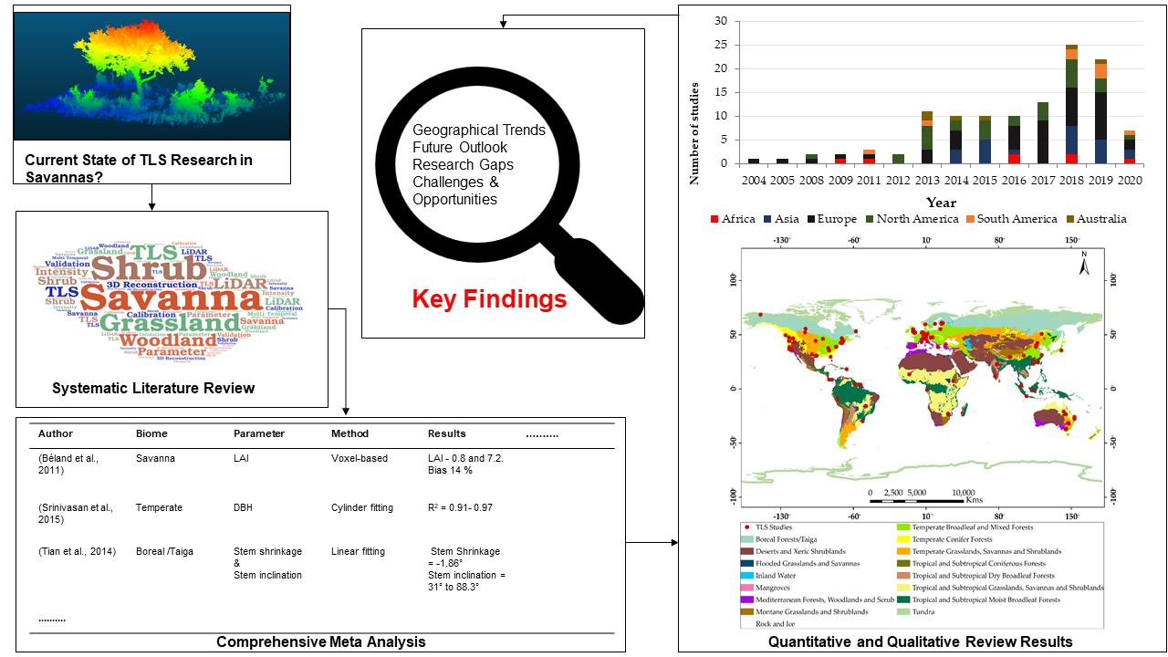
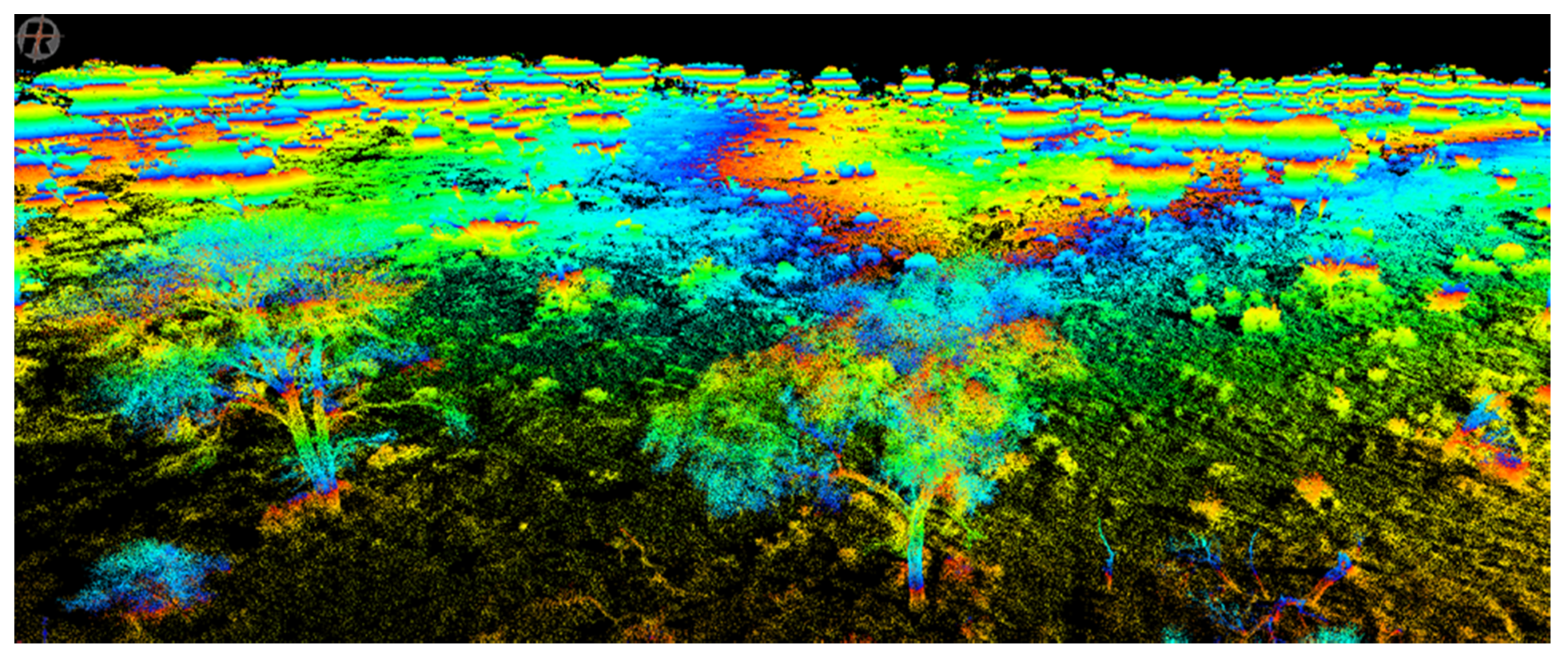
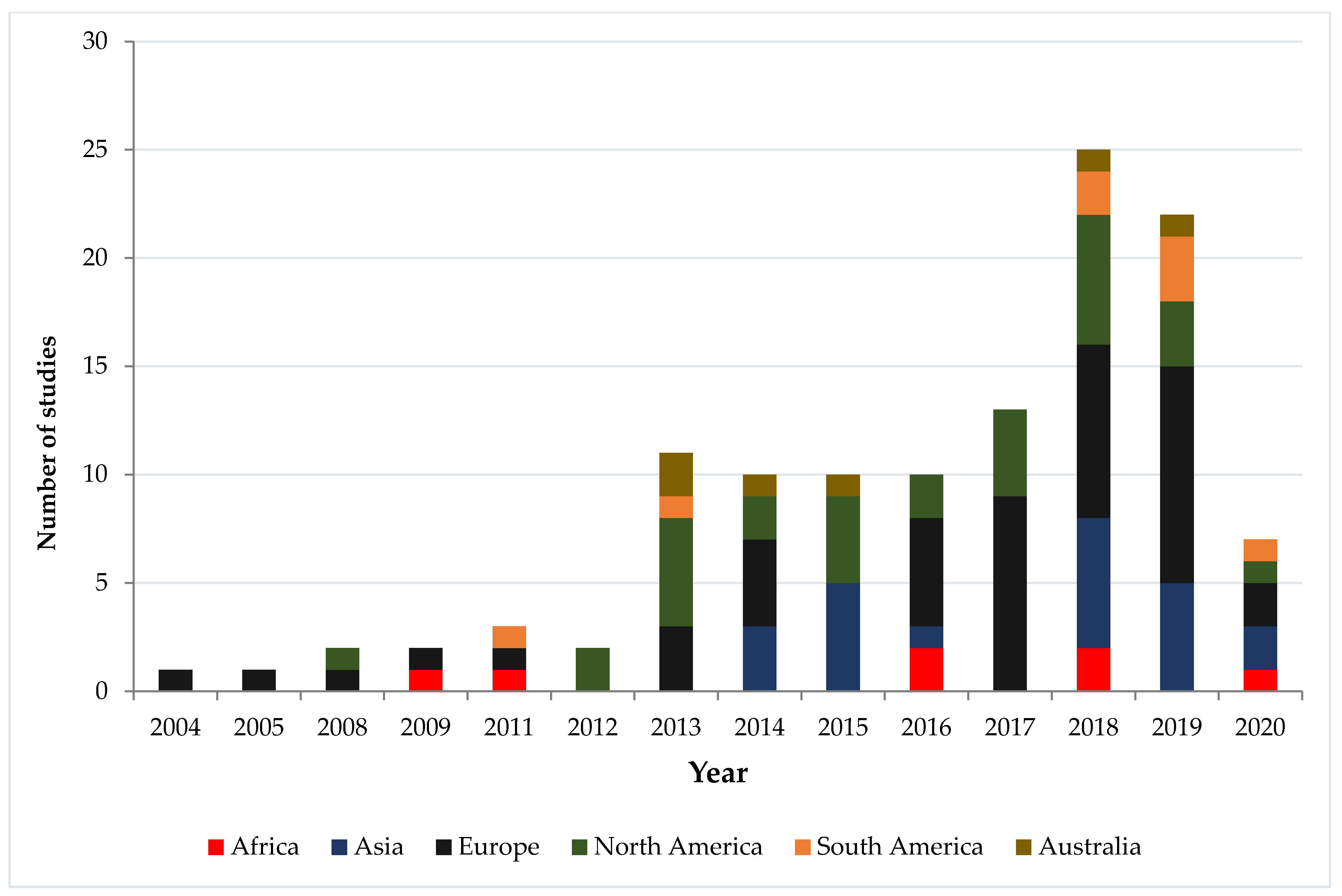
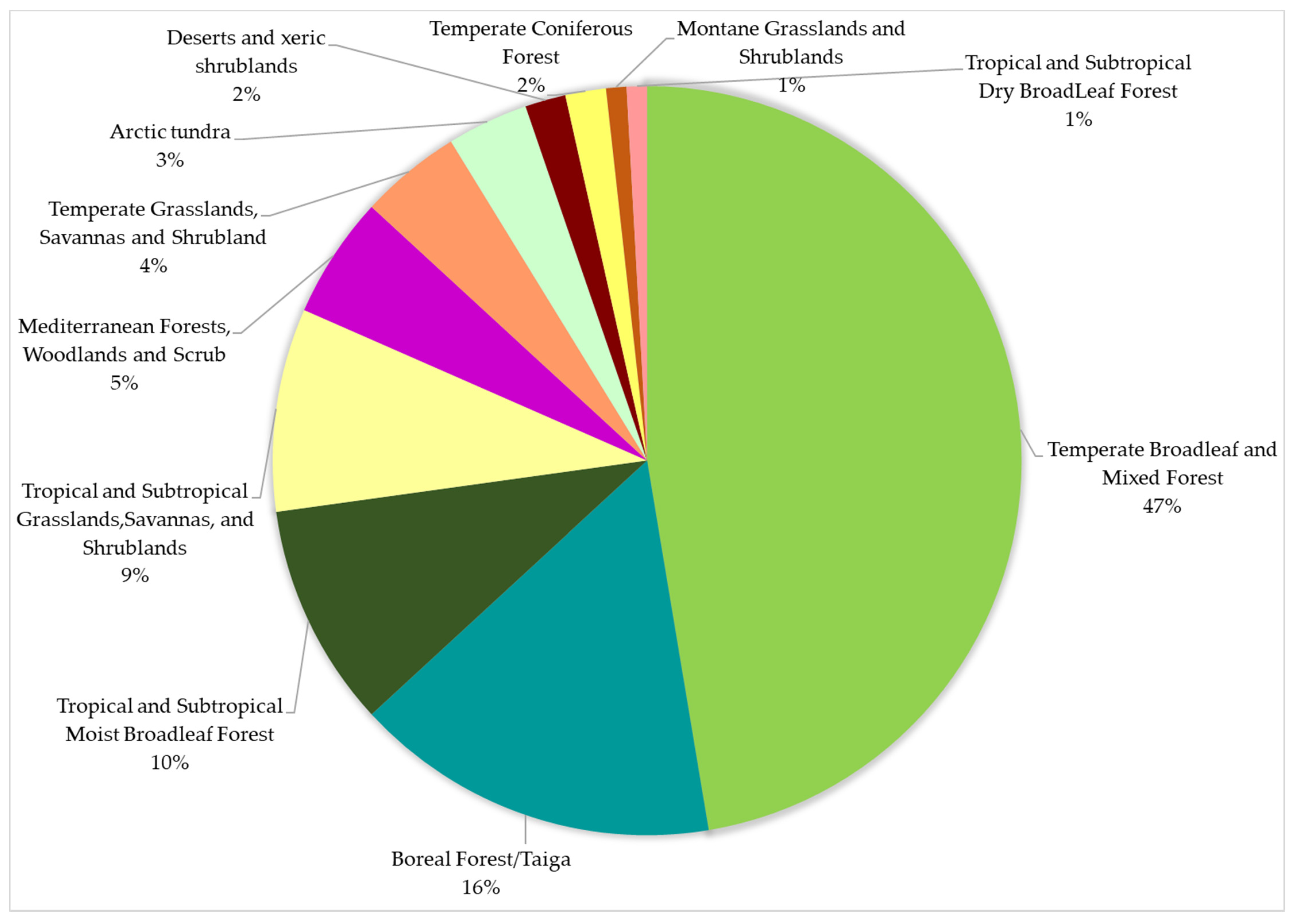
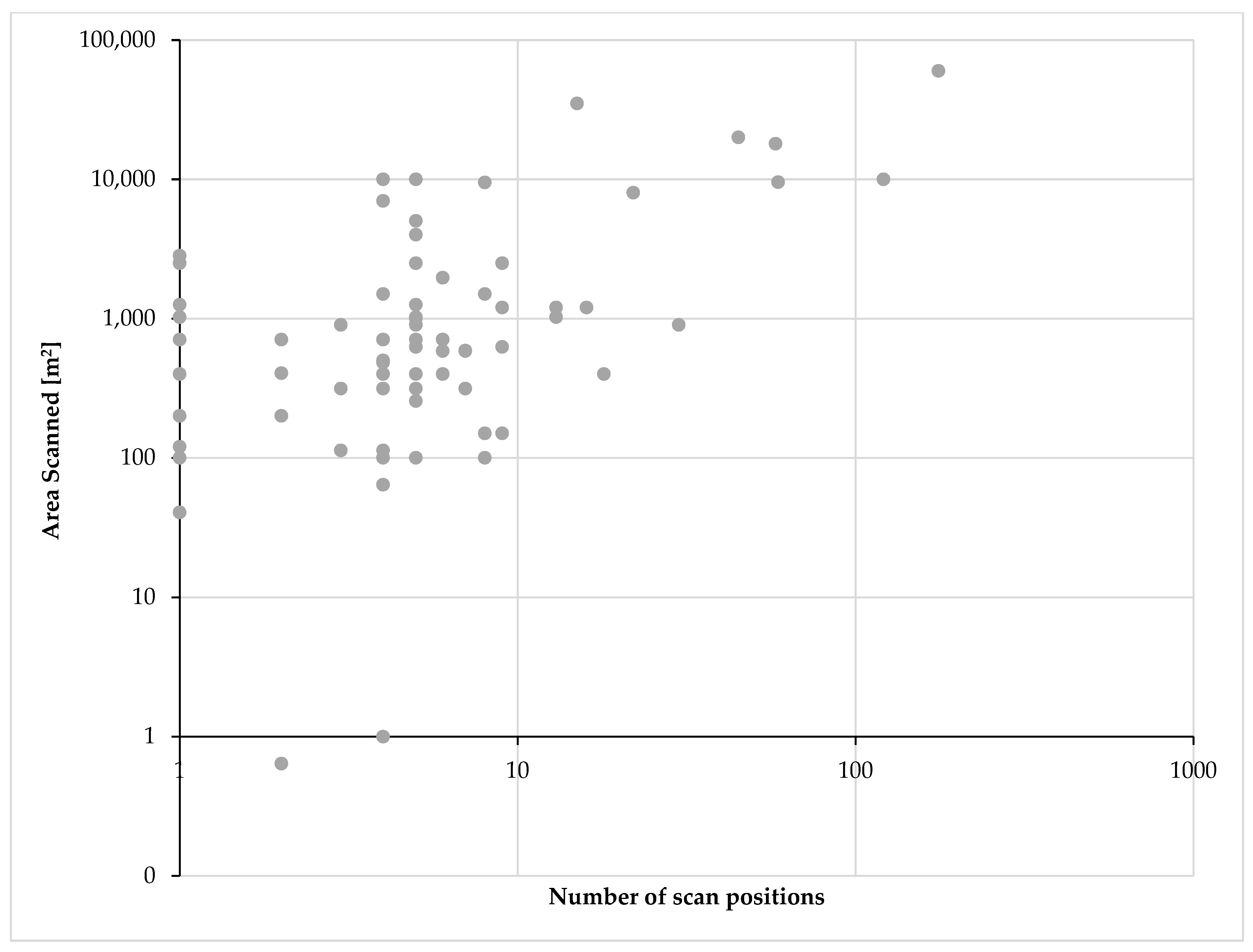
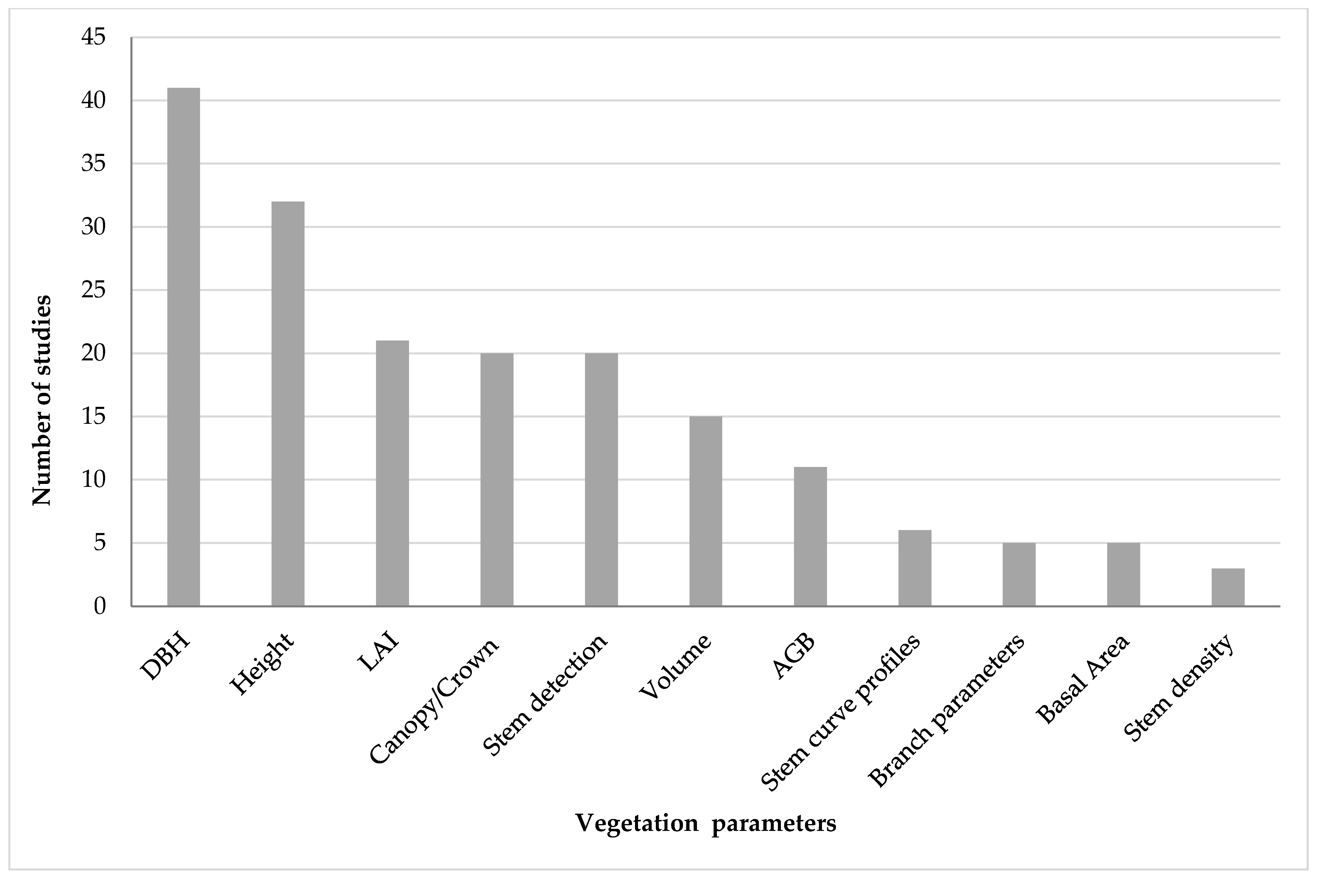
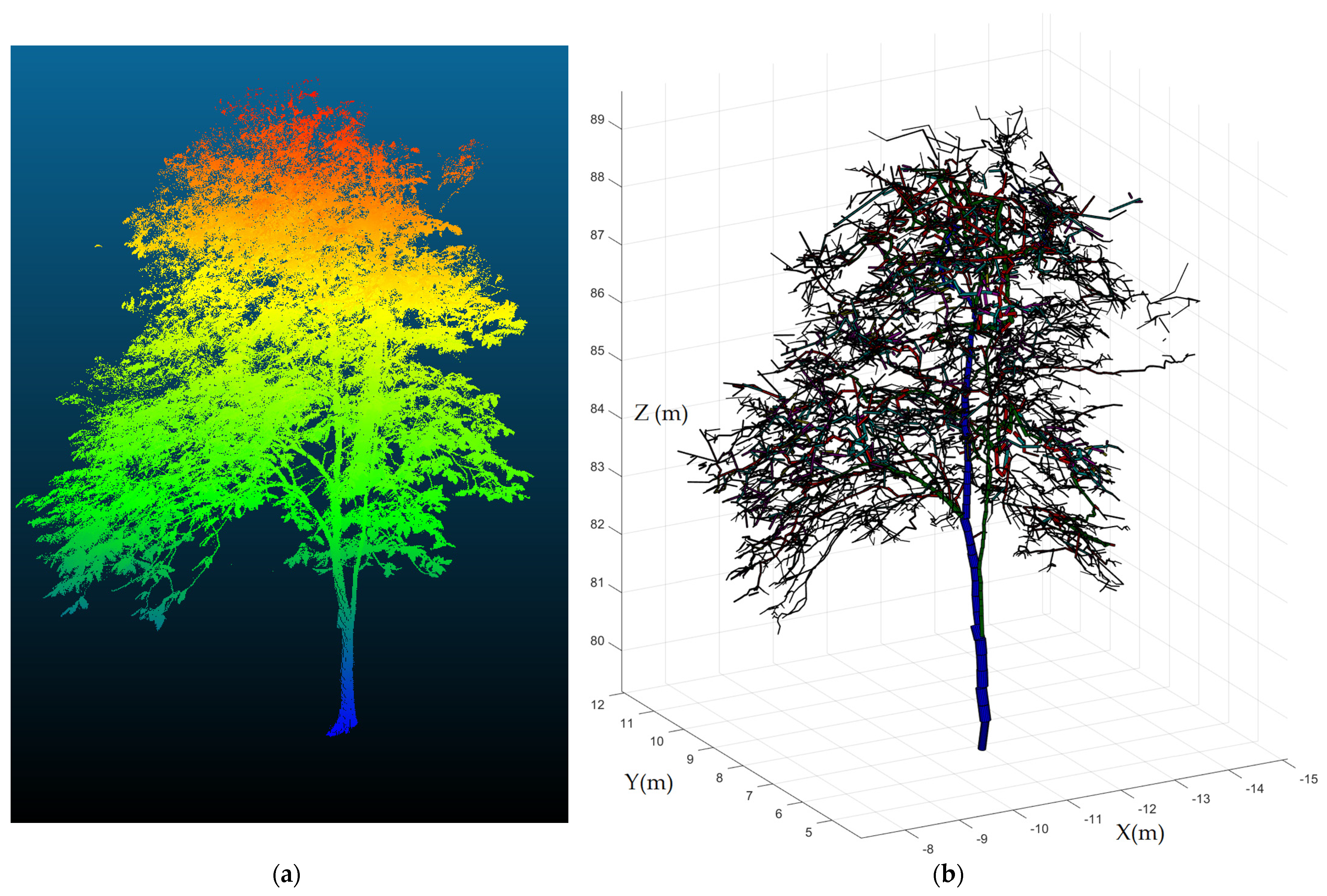
Table 1.
Search terms used to build the search queries for this review.
| Search Aspect | Search Terms |
|---|---|
| Vegetation type | forest *; grassland *; savanna *; shrub *; woodland * |
| TLS | ground-based lidar; lidar; terrestrial laser scann *; terrestrial lidar; TLS |
| Extraction of vegetation parameters | 3D reconstruction; reconstruction; stem; tree parameter; tree structur *; |
| TLS experimental setup | full waveform; intensity; multi-temporal; reflection |
| TLS as auxiliary data | calibration; validation |
Table 2.
Commonly used terrestrial laser scanners.
| Riegl VZ 400 | Leica HDS6100 | Riegl VZ 1000 | Faro Focus 3D | Faro Focus 3D X 330 | |
|---|---|---|---|---|---|
| Range finder | Time of flight | Phase shift | Time of flight | Phase shift | Phase shift |
| Range of Measurement [m] | 1.5–600 | 79 | 2.5–1400 | 0.6–120 | 0.6–330 |
| Scan angle range [°] | 100/360 | 360/310 | 100/360 | 305/360 | 300/360 |
| Accuracy [mm] | 5 | ±2 at 25 m | 8 | ±2 | ±2 |
| Beam divergence[mrad] | 0.35 | 0.22 | 0.3 | 0.19 | 0.19 |
| Laser wavelength[nm] | 1550 | 690 | 1550 | 905 | 1550 |
| Effective measurement rate [points/sec] | 42,000–122,000 | 508,000 | 42,000–122,000 | 122,000–976,000 | 122,000–976,000 |
| Angel measurement resolution[°] | 0.0005° (1.8arc sec) | 0.009° Hor × 0.009° Ver | 0.0005° (1.8arc sec) | 0.011° | 0.011° |
| Weight[kg] | 9.6 | 14 | 9.8 | 5.0 | 5.2 |
| Reference | [116] | [117] | [118] | [119] | [120] |
Publisher’s Note: MDPI stays neutral with regard to jurisdictional claims in published maps and institutional affiliations. |
© 2021 by the authors. Licensee MDPI, Basel, Switzerland. This article is an open access article distributed under the terms and conditions of the Creative Commons Attribution (CC BY) license (http://creativecommons.org/licenses/by/4.0/).
Share and Cite
MDPI and ACS Style
Muumbe, T.P.; Baade, J.; Singh, J.; Schmullius, C.; Thau, C. Terrestrial Laser Scanning for Vegetation Analyses with a Special Focus on Savannas. Remote Sens. 2021, 13, 507. https://doi.org/10.3390/rs13030507
AMA Style
Muumbe TP, Baade J, Singh J, Schmullius C, Thau C. Terrestrial Laser Scanning for Vegetation Analyses with a Special Focus on Savannas. Remote Sensing. 2021; 13(3):507. https://doi.org/10.3390/rs13030507
Chicago/Turabian StyleMuumbe, Tasiyiwa Priscilla, Jussi Baade, Jenia Singh, Christiane Schmullius, and Christian Thau. 2021. "Terrestrial Laser Scanning for Vegetation Analyses with a Special Focus on Savannas" Remote Sensing 13, no. 3: 507. https://doi.org/10.3390/rs13030507
Note that from the first issue of 2016, this journal uses article numbers instead of page numbers. See further details here.