Analyzing Changes in Frozen Soil in the Source Region of the Yellow River Using the MODIS Land Surface Temperature Products


1
School of Water Resources and Environment, China University of Geosciences, Beijing 100083, China
2
China Highway Engineering Consultants Corporation, Space Information Application and Disaster Prevention and Mitigation Technology Transportation Industry R & D Center, China Consulting Data Co., Ltd., Beijing 100089, China
3
College of Hydraulic and Civil Engineering, Xinjiang Agricultural University, Urumqi 830052, China
*
Author to whom correspondence should be addressed.
Remote Sens. 2021, 13(2), 180; https://doi.org/10.3390/rs13020180
Submission received: 24 November 2020
/
Revised: 21 December 2020
/
Accepted: 4 January 2021
/
Published: 7 January 2021
(This article belongs to the Special Issue Remote Sensing Applications for Hydrogeography and Climatology)
Abstract
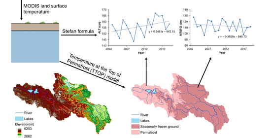
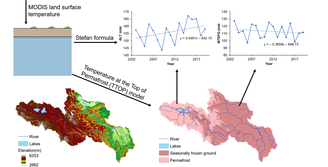
:The degradation of the frozen soil in the Qinghai–Tibetan Plateau (QTP) caused by climate warming has attracted extensive worldwide attention due to its significant effects on the ecosystem and hydrological processes. In this study, we propose an effective approach to estimate the spatial distribution and changes in the frozen soil using the moderate-resolution imaging spectroradiometer (MODIS) land surface temperature products as inputs. A comparison with in-situ observations suggests that this method can accurately estimate the mean daily land surface temperature, the spatial distribution of the permafrost, and the maximum thickness of the seasonally-frozen ground in the source region of the Yellow River, located in the northeastern area of the QTP. The results of The Temperature at the Top of the Permafrost model indicates that the area of permafrost in the source region of the Yellow River decreased by 4.82% in the period from 2003 to 2019, with an increase in the areal mean air temperature of 0.35 °C/10 years. A high spatial heterogeneity in the frozen soil changes was revealed. The basin-averaged active layer thickness of the permafrost increased at a rate of 5.46 cm/10 years, and the basin-averaged maximum thickness of the seasonally-frozen ground decreased at a rate of 3.66 cm/10 years. The uncertainties in calculating the mean daily land surface temperature and the soil’s thermal conductivity were likely to influence the accuracy of the estimation of the spatial distribution of the permafrost and the maximum thickness of the seasonally-frozen ground, which highlight the importance of the better integration of field observations and multi-source remote sensing data in order to improve the modelling of frozen soil in the future. Overall, the approach proposed in this study may contribute to the improvement of the application of the MODIS land surface temperature data in the study of frozen soil changes in large catchments with limited in-situ observations in the QTP.
1. Introduction
‘Frozen soil’ refers to soil and rock containing ice, with a temperature at 0 °C or below 0 °C [1]. According to the time length of the frozen state, frozen soil can be generally divided into two types: seasonally-frozen ground and permafrost. Due to its unique thermal and hydraulic characters, frozen soil plays an important role in the energy and water exchange between the land surface and the atmosphere system [2]. In response to global warming, the degradation of frozen soil has exhibited significant effects on regional hydrological processes, biochemical cycles and land ecosystems [2,3,4]. Therefore, mapping the spatial distribution of frozen soil and monitoring the changes in the soil freezing/thawing state are quite important for water resource management and ecosystem protection in cold regions. Particularly, the maximum thickness of the seasonally-frozen ground (MTSFG), which is the maximum value of the thickness of the frozen soil layers (the common unit of MTSFG used for observation is cm) in the seasonally-frozen area, and the active layer thickness (ALT) of the permafrost are the most frequently-investigated variables. China has the largest area of high-altitude permafrost, which is mostly located on the Qinghai–Tibetan Plateau (QTP). The QTP is also the source region for many important Asian rivers, such as the Yangtze River, the Mekong River, and the Yellow River [5]. The significant effects of the changes in the permafrost and the seasonally-frozen ground on catchment hydrological processes have been reported [6,7,8,9], and such changes have also caused an evident shift in the ecosystems on the QTP [10,11,12]. Thus, the estimation of the changes in the frozen soil is essential for the prediction of the response of land surface processes to climate change on the QTP.
Traditional studies on frozen soil have mainly relied on field observations. However, due to the cold climate, in-situ observations are usually sparse in frozen-ground regions. Therefore, great difficulties are entailed for the mapping of the spatial distribution of the frozen soil relying on the in-situ observations at the plot scale, particularly in the vast QTP and its complex landscapes. Various methods have been developed for mapping and simulating the spatial distribution and changes in frozen soil at the regional scale. Some researchers have simulated frozen soil processes using physically-based distributed models. For example, Wania et al. [13] developed the Lund–Potsdam–Jena Wetland Hydrology and Methane Model, and simulated the distribution of the permafrost in the high latitude region. Guo et al. [14] investigated the frozen soil changes on the QTP using the Community Land Model. Gao et al. [8] simulated the changes in frozen soils in the upper Heihe River Basin using the Geomorphology-Based Ecohydrological Model. However, these physical models need a large amount of input data and computational complexity, which causes limitations for their application at the regional scale. Some studies utilized the machine learning method in order to estimate the spatial distribution of frozen soil [15,16]. However, the machine learning approach is a ‘black box’ model which does not consider the physical interactions between frozen soil and the environmental factors, which may pose large uncertainties, such like overfitting in the training period and poor performance in the testing period. On the other hand, the machine learning method also needs a large amount of observed data for the training of the model. Thus, it is difficult to apply the machine learning method in cold regions with sparse observations. Therefore, with less requirement for computational resources and great efficiency, analytical models based on the simplified physical relationship between the frozen soil and environmental factors are a practical choice. For example, The Temperature at the Top of Permafrost (TTOP) model [17] and the Stefan formula [18] have shown high accuracy in simulating the distribution of the permafrost, as have the changes in the MTSFG and the ALT of the permafrost in the QTP in the previous studies [7,19,20]. The TTOP model is an approach which identifies permafrost by estimating the mean annual temperature at the top of perennial frozen/unfrozen soil using a function of the thermal offset effect with freezing and thawing indices at the ground surface. The Stefan formula is a simplified solution of the exact equation for the moving phase change boundary using accumulated ground surface degree days [21].
The traditional analytical model applied in cold regions also relies on sparse observed data as its input, which restricts its application, although it has a high efficiency. With the rapid development of the remote sensing method in recent years, high quality remote sensing data with fine spatial resolution could be used to drive the analytical model. Land Surface Temperature (LST) is one of the most important factors affecting the distribution of frozen soil, because it is the upper boundary of the soil freezing/thawing processes. LST has proven to be excellent in estimating the thermal state and the ALT of the permafrost [22,23]. However, in cold regions, the in-situ observations of the LST are quite sparse in their distribution, particularly in the QTP. In recent years, satellite remote sensing has gradually become an effective method to obtain the high spatial and temporal distributions of the regional LST, making it possible to estimate the distribution of the frozen soil based on remote sensing [24,25,26,27]. For example, Zou et al. [26] used the MODIS LST products to simulate the permafrost distribution on the QTP, and the results showed that the application of MODIS LST products could improve the accuracy of the mapping of the permafrost on the QTP. However, studies on the frozen soil changes at the regional or catchment scale in the QTP are still lacking, and few studies have investigated the changes in the frozen soil distribution, ALT, and MTSFG at the catchment scale using remote sensing.
The source region of the Yellow River (SRYEARS) is located on the northeastern QTP, and provides about one third of the total runoff of the Yellow River. Frozen soil changes are considered to have significant effects on the vegetation dynamics and river discharge in the SRYEARS [20,28,29,30]. Therefore, the analysis of the spatial and temporal changes in the frozen soil are important for the water resources management and ecosystem protection in the SRYEARS.
The objectives of this study are: (1) to evaluate the applicability of the Stefan equation and TTOP model driven by the remote sensing LST; (2) to estimate the changes in the spatial distribution of the frozen soil, ALT, and MTSFG in the SRYEARS in the period from 2003 to 2019; and (3) to quantify the uncertainties in the analytical model based on remote sensing.
2. Study Area and Data
2.1. Study Area
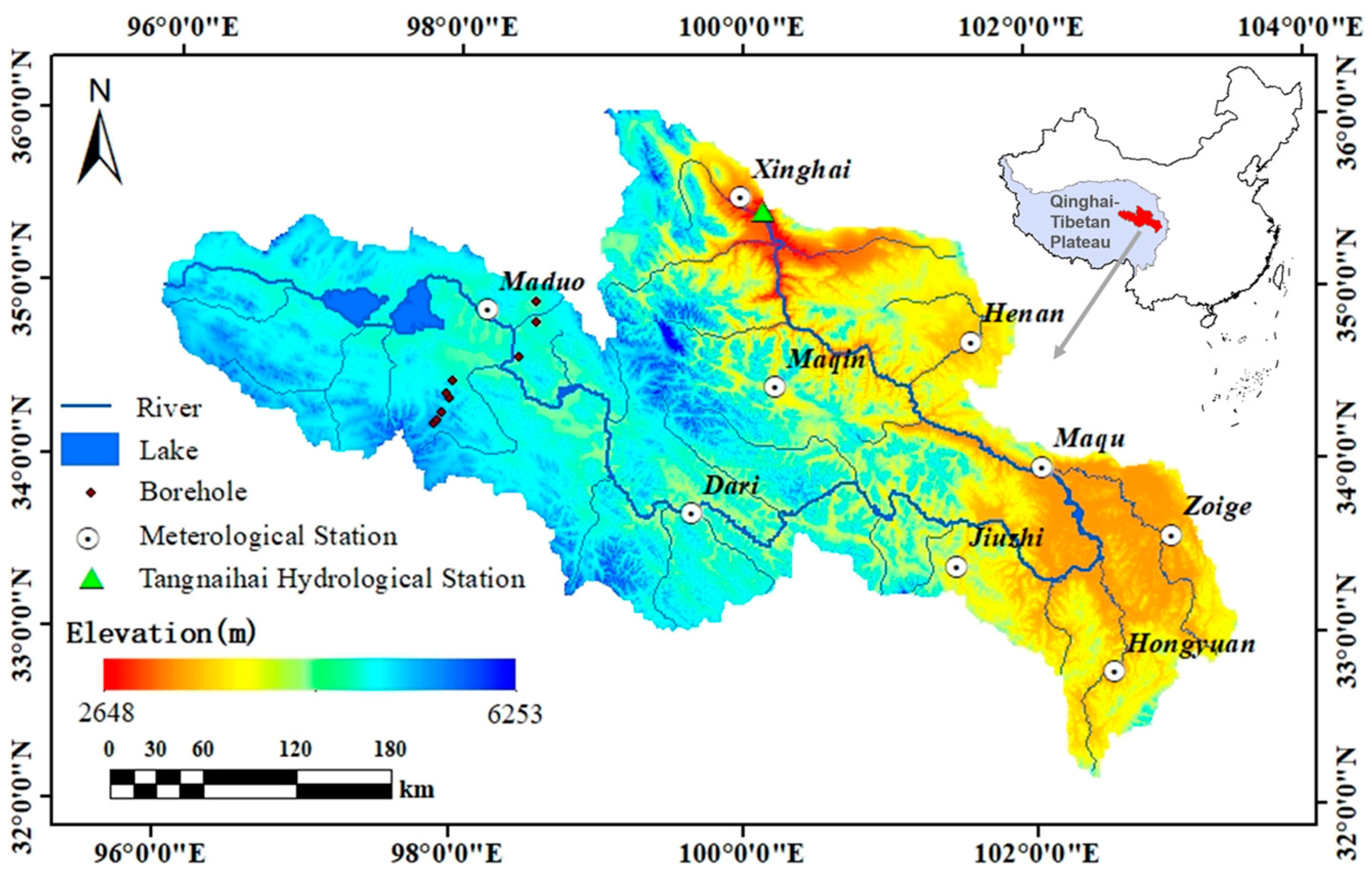
In this study, the SRYEARS refers to the drainage area upstream of the Tangnaihai Hydrological Station. With an area of 12.37 × 10⁴ km2, the SRYEARS accounts for 16.2% of the total area of the Yellow River, but it provides 35% of the total runoff volume of the Yellow River [20]. The SRYEARS is located in the transitional zone between the seasonally-frozen ground and the permafrost on the northeastern QTP [20]. The elevation of the SRYEARS ranges from 2648 to 6253 m (Figure 1), with a descending tendency from west to east.
2.2. Data
The MODIS LST data in the 2003–2019 period were provided by the National Aeronautics and Space Administration (NASA) (https://ladsweb.modaps.eosdis.nasa.gov/). This includes the clear-sky MOD11A2 (Terra MODIS) and MYD11A2 (Aqua MODIS) products, with a spatial resolution of 1 km and an 8-day time interval. The MOD11A2 and MYD11A2 data both provide two remote sensing observations (daytime and nighttime) within a given day. Therefore, there are four remote sensing observed LST data within a given day for the same pixel.
The meteorological data used in this study includes the observed daily air temperature and the precipitation data at nine stations (Figure 1) and the gridded daily precipitation data [31] in the SRYEARS during the period of 2003–2019, with a spatial resolution of 0.25 degree. This gridded precipitation data was downloaded from the website of the China Meteorological Administration (CMA) (http://data.cma.cn), and it was resampled to a 1 km × 1 km grid system in order to match the spatial resolution of the MODIS LST data.
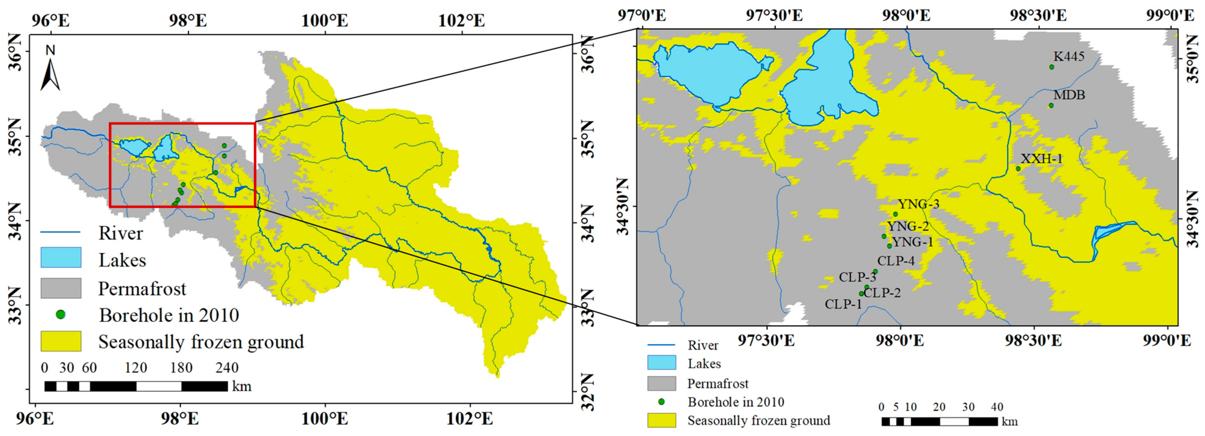
The observed mean daily LST and the daily frozen depth data were also provided by the CMA. The observed frozen depth is used to calculate the MTSFG, and it is available in the period from 2003 to 2015 (see Table 1), with the exception of the Maqu station, which only has observations from 2007 to 2015. The observed LST data is available in the same period as the observed meteorological data. The observed frozen soil types at 10 boreholes in 2010 (Figure 2) provided by Luo et al. [32] were used to validate the spatial distribution of the frozen soil estimated in this study.
The soil property data used in this study were obtained from the Harmonized World Soil Data (HWSD) [33], which includes the soil sand content, the clay content and the soil bulk density, and it has a spatial resolution of 0.00833 degrees, which is approximately the same as MODIS LST data. This data was provided by the Food and Agriculture Organization of the United Nations (FAO), and was downloaded from the website of the National Tibetan Plateau Data Center (NTPDC) (http://data.tpdc.ac.cn). The saturated soil moisture content data (which also has a spatial resolution of 0.00833 degrees) was provided by Dai et al. [34]. The 0–100 cm depth soil moisture data were derived from the China Soil Moisture Dataset from Microwave Data Assimilation (CSMDA) (http://en.tpedatabase.cn), and they have a spatial resolution of 0.25 degrees.
3. Methodology
3.1. Estimating the Mean Daily LST Using MODIS Data
The MODIS LST product represents instantaneous remote sensing observations at four overpass times in a day (Beijing time: 1:30, 10:30, 13:30, and 22:30). Therefore, a method is needed to estimate the mean daily LST using these four different remote sensing observations within a day. Most previous studies used an arithmetic mean of the four remote sensing observations to estimate the mean daily LST. However, due to the nonlinear characteristics of the diurnal cycle of the LST, the arithmetic mean of the four LST remote sensing observations produces large errors for the estimation of the mean daily LST [35]. Therefore, a multiple linear regression method with different weights for each MODIS remote sensing observations was adopted to estimate the mean daily LST in this study. The whole year was divided into two seasons: the warm season (from May to August) and the cold season (from September to April of the following year). The coefficients of the regression model in the two seasons were calibrated using the observed LST at the nine meteorological stations in the SRYEARS during the period of 2003–2019 (Table 1). The average daily LST of the same 8-day interval as the MODIS data observed at each station was compared with the MODIS LST of the grid in which the station is located. Then, the regression coefficients obtained at each station were averaged in order to obtain the coefficients of the final equations for the whole SRYEARS, which are shown as follows:
where LSTc is mean daily LST (°C) in the cold season (from September to April of the following year), and LSTw is the mean daily LST (°C) in the warm season (from May to August). Terraday and Terranight are the daytime and nighttime LST data (°C) of the MOD11A2, respectively, and Aquaday and Aquanight are the daytime and nighttime LST data (°C) of the MYD11A2, respectively. The grounds of the meteorological stations are mainly covered by alpine meadow and alpine steppe (Table 1). Therefore, the MODIS LST is the ‘skin temperature’ influenced by the vegetation canopy in the warm season, and by the litter layer or snow cover in the cold season. However, the LST at the meteorological stations is the ground surface temperature (GST), which is observed by the sensors of a thermometer half buried in the ground, and it approximately represents the 0 cm surface temperature. Thus, the MODIS LST is colder than the observed LST at the meteorological stations. This difference partially explained the high intercepts obtained in Equations (1) and (2), which may offset the cold bias of the MODIS LST.
The mean error (ME) and the root mean square error (RMSE) were used to evaluate the accuracy of the mean daily LST estimated using Equations (1) and (2) at the nine stations. The ME and RMSE were calculated as follows:
where n is the number of observations, i is the observation number, and y is the mean daily LST.
3.2. Estimating the Distribution of Permafrost
In this study, the TTOP model was adopted in order to estimate the distribution of the permafrost. The value of TTOP was calculated as follows [17]:
where kt is the thermal conductivity of thawed soil (W·m−1·°C −1), DDT and DDF represent degree days, DDT is the ground surface thawing index (°C day), kf is the thermal conductivity of frozen soil (W·m−1·°C−1), DDF is the ground surface freezing index over a freezing year (°C day), and P is the annual period (365 days). A freezing year is defined as being from July to the June of the following year. For each grid, DDF was calculated by summing up all of the daily mean ground surface temperatures lower than 0 °C in a freezing year, and DDT was calculated by summing up all of the daily mean ground surface temperatures higher than 0 °C in a normal year. Equation (5) indicates that if the sum of the ground temperature during the freezing period is greater than that in the thawing period within a freezing–thawing cycle, the TTOP value is negative, indicating that permafrost exists. The distribution of frozen soil was determined as follows:
In Equation (5), the thermal conductivity of the soil was calculated using Johansen’s scheme [36], as follows:
where ksat and kdry are the thermal conductivities of the soil in a saturated state and dry state (W·m−1·°C−1), respectively. ksat was calculated as follows:
where λω and λi are the thermal conductivities of water (0.57 W·m−1·K−1) and ice (2.2 W·m−1·K−1), respectively; Tf is the freezing point, and λs is the thermal conductivity of solid particles, which was calculated as follows:
where λq and λ0 are the thermal conductivities of quartz (7.7 W·m−1 °C−1) and all other minerals (2.0 W·m−1·°C−1), respectively. δ is the volumetric fraction of quartz, which can be determined as half of the sand content [35]. kdry in Equation (7) was calculated as follows [36]:
where is the bulk density. Ke in Equation (7) was estimated as follows:
where Sr is the degree of saturation, θliq is the liquid soil water content (m3·m−3), and θsat is the saturated soil moisture (m3·m−3). In the thawing season, θliq was estimated according to the precipitation, as follows [20]:
where θliq,t is the liquid soil water content in the thawing period (m3·m−3); Pm is the monthly precipitation (mm) in the thawing period, which is calculated in September, August, and July, respectively; and αt and c are regression coefficients, which are calibrated by the average 0–100 cm soil water contents (July–September) during the period of 2002–2010, from the CSMDA dataset. The average liquid soil water content θliq in the freezing period was calculated as follows:
where θliq,f is the liquid soil water content in the freezing period (m3·m−3); Ds is the reference thickness of soil layer, which is assigned as 2.0 m according to the Second National Soil Survey [7]; and Pf (t) is the preceding precipitation index before the freezing period, which was calculated as follows:
where αf is the recession coefficient, which is calibrated as 0.95.
In this study, the soil thermal conductivity calculation by Kersten’s scheme [37] was also compared with the results of Johansen’s scheme. In Kersten’s scheme, the soil thermal conductivity of thawing soil is calculated as follows:
The thermal conductivity of frozen soil is calculated as follows:
where ω is the soil moisture content (%), and is the soil bulk density (kg m−3). Both ω and were measured by soil samples collected in the field survey by Li et al. [38]. These soil samples were classified according to soil type; the soil moisture content and bulk density values were averaged within the soil types in order to eliminate abnormal values [38].
3.3. Estimating the Maximum Thickness of the Seasonally-Frozen Ground and the Active Layer Thickness of the Permafrost
The MTSFG and ALT were calculated using the Stefan formula [18], as follows:
where MTSFG and ALT are the maximum thickness of the seasonally-frozen ground (m) and the active layer thickness (m) of the permafrost, respectively. nt and nf are parameters. When DDF and DDT are calculated using LST, the value of nt and nf are both 1. τ is the time length (8.64 × 10⁴ s·day−1); L is the latent heat of fusion (3.34 × 10⁵ J·kg−1); ρω is the liquid water density (103 kg·m−3); and θliq,t and θliq,f are the average liquid soil water content (m3·m−3) in the thawing period and freezing period, respectively, which were calculated using Equations (12)–(14).
4. Results
4.1. Validation of the Mean Daily LST Estimated by Remote Sensing
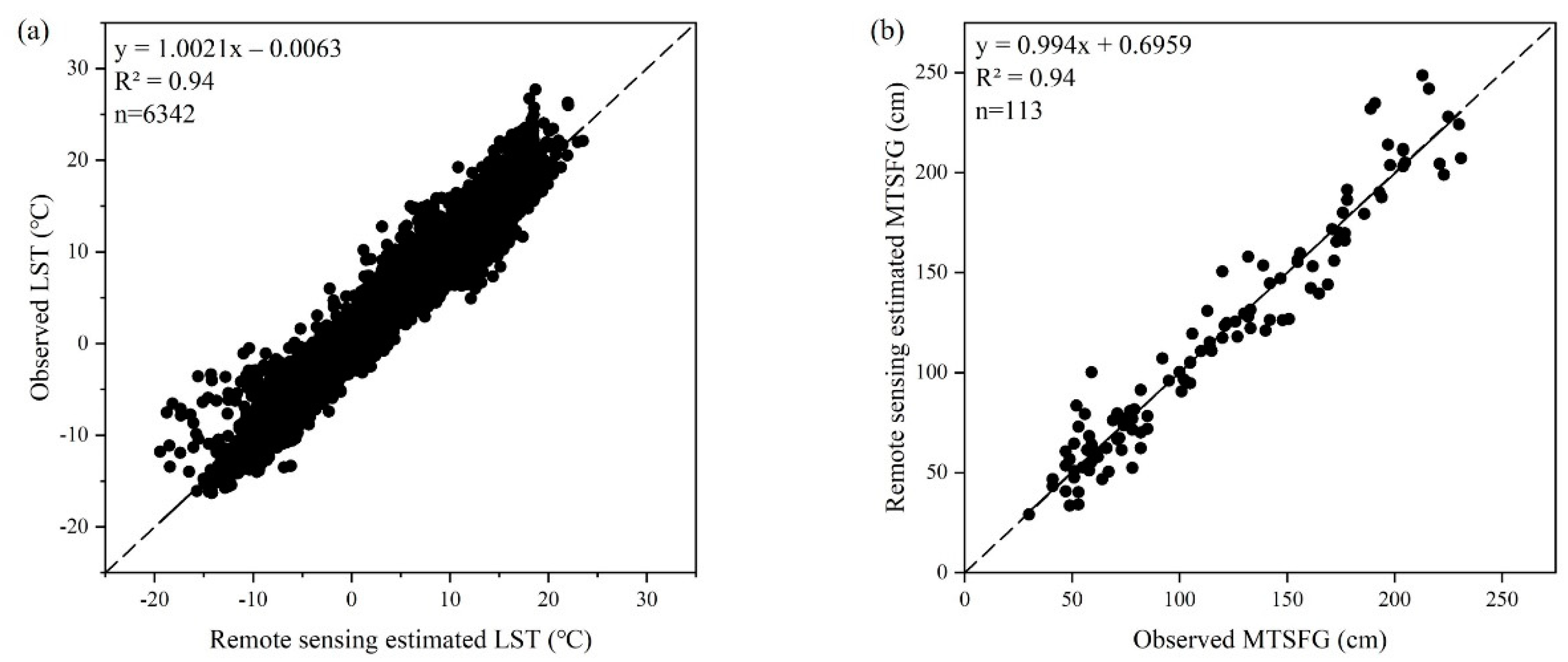
Figure 3a and Table S1 in the Supplemental Material show that the mean daily LST estimated using Equations (1) and (2) agrees well with the observations at all of the stations. The R2 ranged from 0.92 to 0.96, the ME ranged from −0.46 to 0.54 °C, and the RMSE ranged from 1.91 to 2.27 °C (Table S1). These results indicate that Equations (1) and (2) showed acceptable accuracy in estimating the mean daily LST. Therefore, it is reasonable to estimate the mean daily LST at each grid using Equations (1) and (2) based on the MODIS data. Then, the value of DDT and DDF at each grid were calculated using the estimated mean daily LST.
4.2. Validation of the Simulated Distribution of the Permafrost by Remote Sensing
The observations of the frozen soil types at 10 boreholes in 2010 [32] were compared with the results estimated by the TTOP model (Figure 2). Table 2 shows that the TTOP model correctly identified the frozen soil types at all of the boreholes. This result illustrates that the method developed in this study is applicable to the estimation of the distribution of frozen soil in the SRYEARS.
4.3. Validation of the MTSFG Estimated by Remote Sensing
The observed MTSFG data in the period from 2003 to 2015 at the nine stations were used to validate the remote-sensing–estimated MTSFG. Figure 3b shows that the fitted linear trend line between the observed and remote-sensing–estimated MTSFG was close to the 1:1 line, indicating a good agreement (R2 = 0.94). The inter-annual variations of the remote sensing estimated MTSFG were generally consistent with the observations (Figure 4). The worst performances of our method were found at the Maduo station and the Maqu station. The Maduo station is located in a region with high elevation, and it has more complex topography than the other stations. Therefore, the errors in the estimation of the MTSFG at this station may be related to the effect of sub-grid topography on the LST which was not well described by the 1 km MODIS data. The annual precipitation at the Maqu station is about 610 mm [11], which is greater than most of the other stations. The relatively high soil moisture content caused by high precipitation at this station greatly influenced the MTSFG. Therefore, the errors at this station may be caused by the uncertainties in the soil moisture estimation using the empirical equations (Equations (12)–(14)). Table S2 in the Supplemental Material shows that both the observed and remote-sensing–estimated MTSFG increased when the elevation increased. The mean value of the remote-sensing–estimated MTSFG was close to the observations. The absolute value of the ME was less than 6 cm at most stations. Almost all of the stations had RMSE values less than 20 cm, except for the Maduo station, which had an RMSE of 20.6 cm. These results illustrate that the method proposed in this study has a high accuracy for the estimation of the MTSFG.
4.4. Historical Change in the Frozen Soil
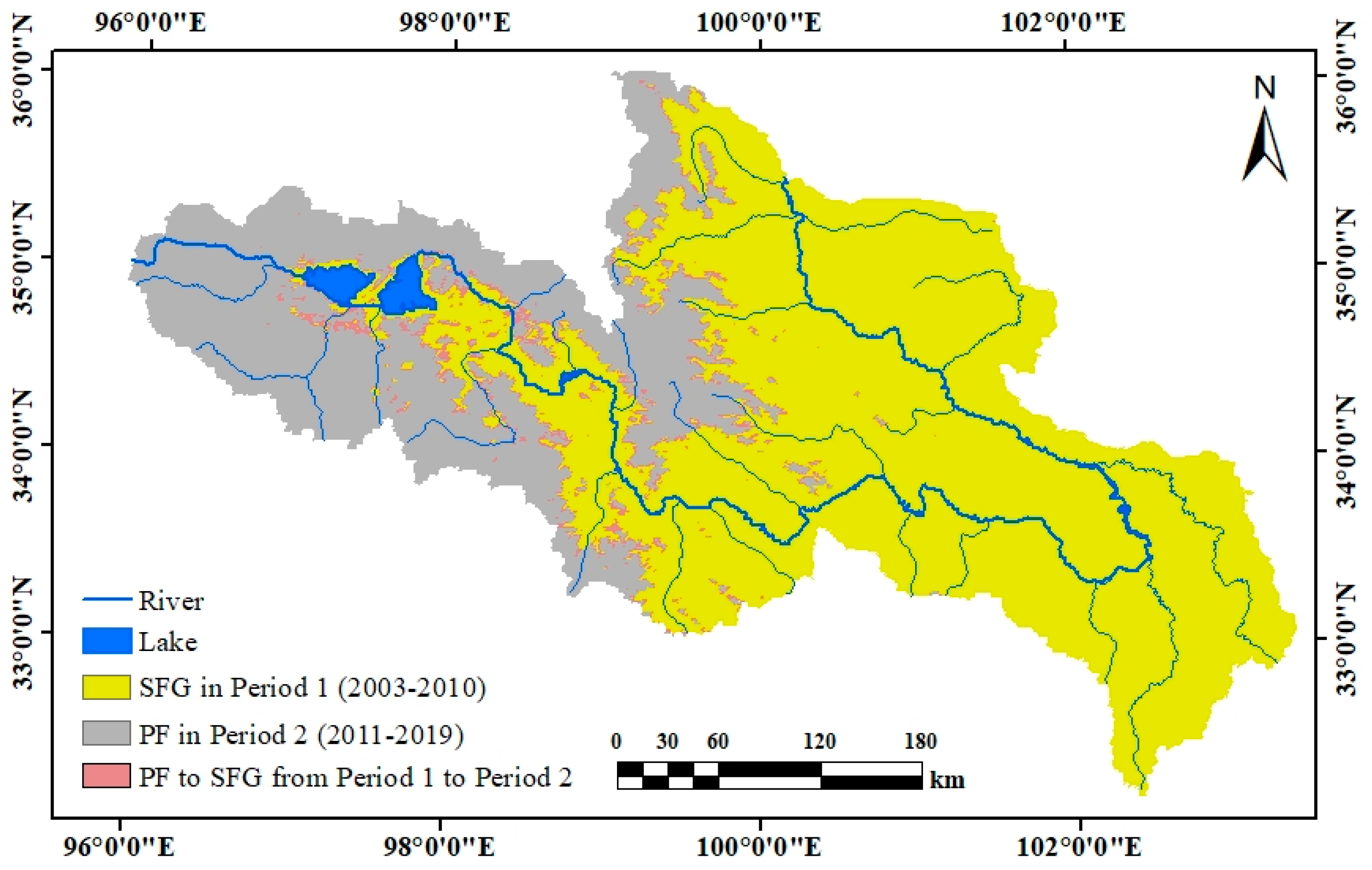
The changes in the distribution of the permafrost in the SRYEARS in two periods—2003–2010 (period 1) and 2011–2019 (period 2)—were estimated using the TTOP model. Figure 5 shows that part of the permafrost in period 1 degraded into seasonally-frozen ground in period 2. In period 1, the area of the permafrost in the SRYEARS was estimated as 35,898 km2, and it decreased to 34,246 km2 in period 2, accounting for a 4.82% decline.
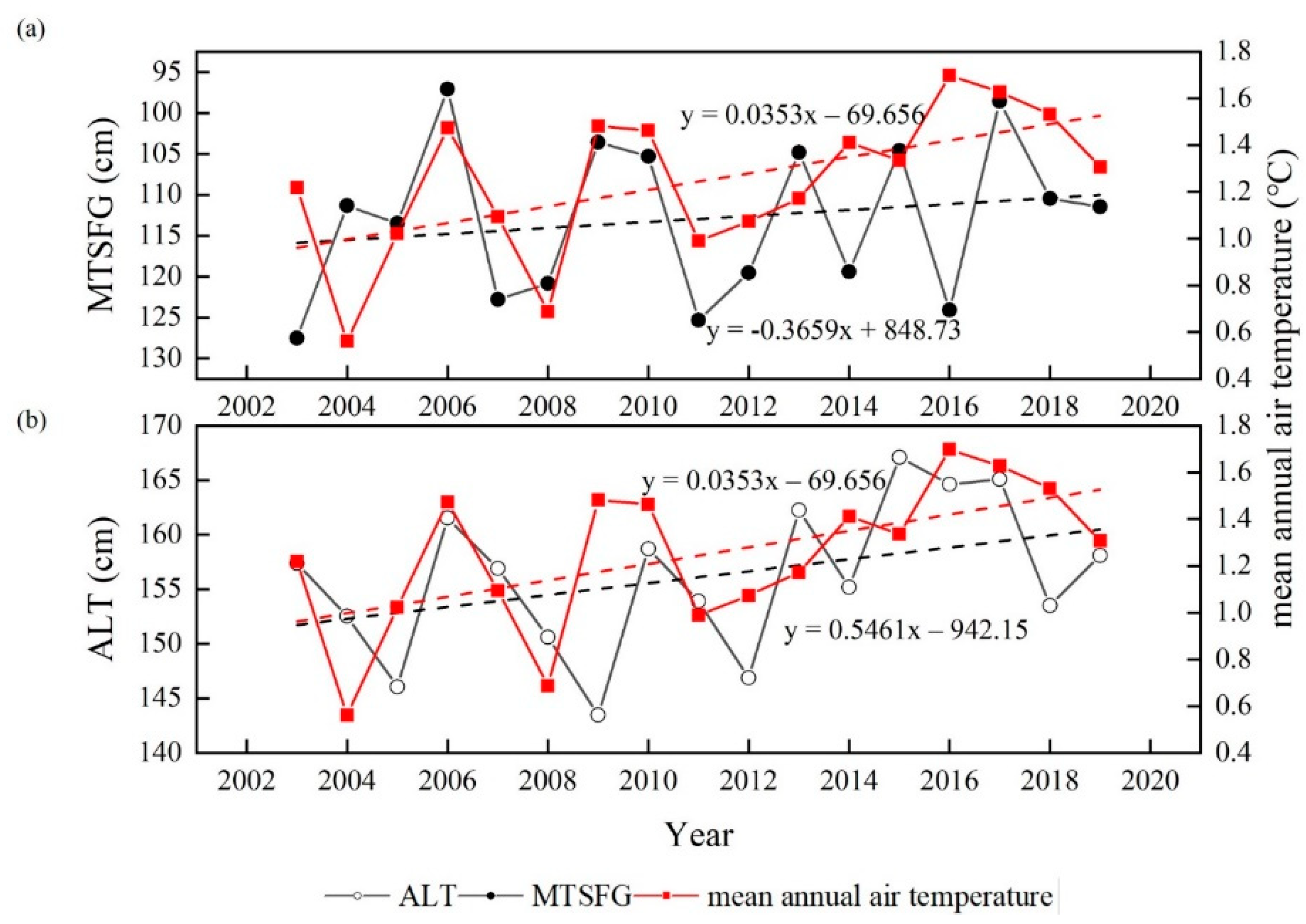
Figure 6 shows the changes in the basin-averaged annual MTSFG and ALT of the permafrost estimated by remote sensing. The basin-averaged annual MTSFG decreased from 127.5 cm in 2003 to 111.5 cm in 2019 at a linear rate of −3.66 cm/10 years. The basin-averaged annual ALT showed an increasing trend with a linear rate of 5.46 cm/10 years, which was consistent with the increase in the mean annual air temperature (MAAT) in the SRYEARS (0.35 °C/10 years). The variations of the MTSFG and ALT had similar patterns to the MAAT. These results suggest that the increasing air temperature had a significant effect on the changes in the frozen soil in the SRYEARS.
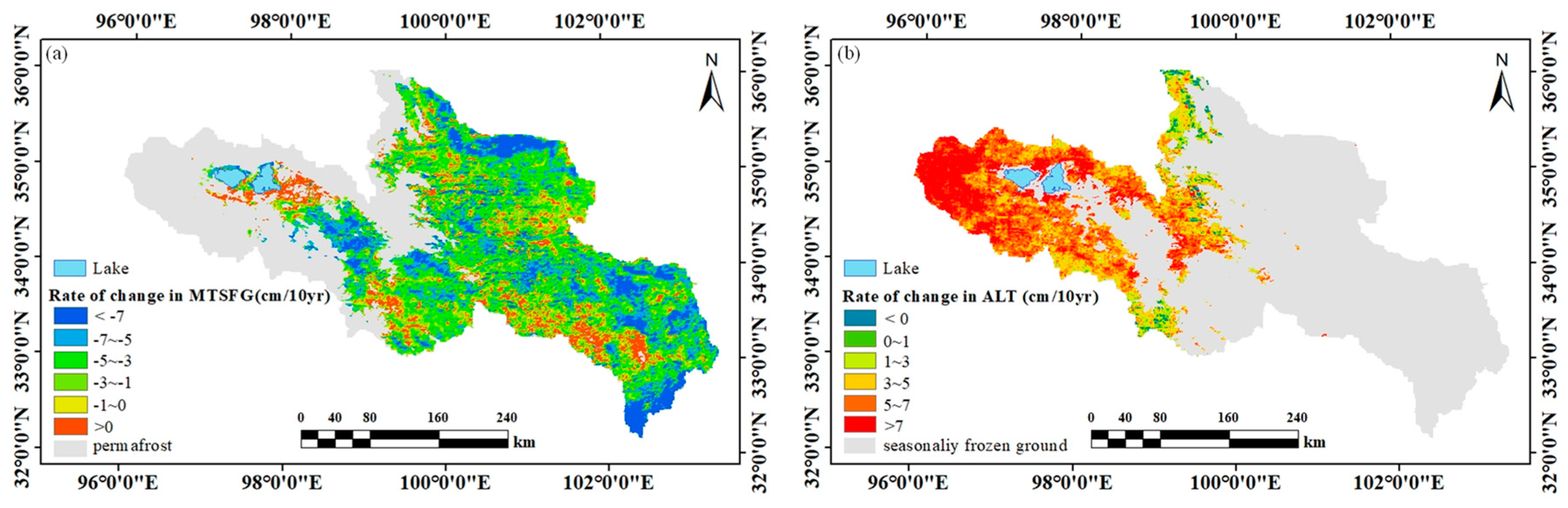
Figure S1 in the Supplemental Material shows the spatial variations of the mean value of MTSFG and ALT estimated by remote sensing in the period from 2003 to 2019. The mean MTSFG ranges from 50 to 190 cm, and it generally declines from west to east as the elevation decreases. The mean value of the ALT ranges from 66 to 208 cm with a basin-averaged value of 156 cm, and it has an eastward-increasing tendency as the elevation decreases. The large spatial variations of the frozen soil changes are illustrated in Figure 7. The MTSFG decreased in most regions during the period of 2003–2019 (Figure 7a). The most significant decreasing trends in the MTSFG were detected in the northern part of the SRYEARS, near the Xinghai station, and in the southeastern part, near the Hongyuan station, with a maximum rate of 34.2 cm/10 years. The ALT of the permafrost increased in most regions (Figure 7b). The largest increase in the ALT was found in the high mountain regions, with a maximum rate of 31.3 cm/10 years.
4.5. Sensitivity Analysis of the Different Parameterizations for the Mapping of the Frozen Soil
In this study, the TTOP model driven by the remote-sensing–estimated LST was used to estimate the spatial distribution and changes in the frozen soil. The different parameterizations for soil thermal conductivity and the estimation of the mean daily LST may influence the results, which were rarely analyzed in previous studies. In order to investigate the sensitivity of the different parameterizations to our results, three experiments—exp1, exp2 and exp3—were designed (Table 3). In exp1, the soil’s thermal conductivity was estimated using Kersten’s scheme; the other variables were estimated in the same manner as in the normal run. In exp2, the coefficients for the estimation of the daily mean LST were derived from Wang et al. [20] which are shown in Table 3, and the other parameters were the same as in the normal run. In exp3, the coefficients in the regression equation for the estimation of the mean daily LST were set to a constant value of 0.25, and the other parameters were the same as in the normal run. Therefore, in exp3, the mean daily LST was the averaged value of the MODIS LST data observed at four different times within a day.
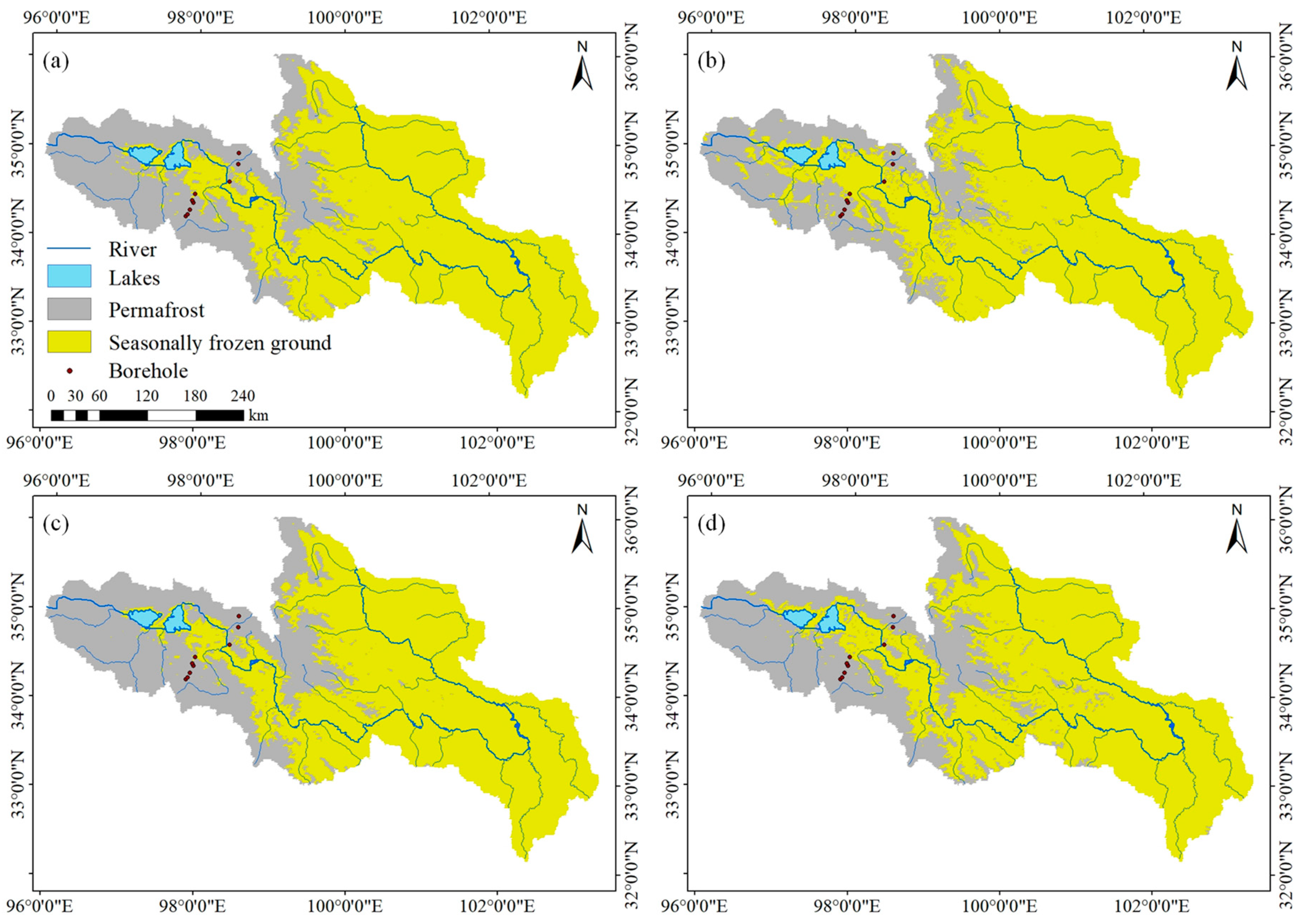
Figure 8b shows that the area of permafrost estimated in exp1 was significant lower than the results of the normal run shown in Figure 8a (also shown in Figure 2), which implies that Kersten’s scheme underestimated the areas of permafrost, and it incorrectly identified the type of frozen soil near the YNG-1 borehole (Table 4 and Figure S2b). In Kersten’s scheme, the soil moisture is set to a constant, and in Johansen’s scheme, the temporal variations of the soil moisture are considered. Therefore, the difference of the results between exp1 and the normal run imply that the consideration of the temporal changes in the soil moisture may be necessary in order to map the frozen soil using remote sensing.
The areas of permafrost estimated in exp2 and exp3 (Figure 8c,d) were larger than the results of the normal run (Figure 2 and Figure 8a), which led to an incorrect identification of the frozen soil type near the YNG-2 borehole (Table 4 and Figure S2c,d). These results indicate that the spatial distributions of the permafrost were sensitive to the regression coefficients for the estimation of the mean daily LST. Uncertainties in mean daily LST estimation can greatly influence the accuracy in the mapping of the frozen soil. The regression coefficients for the estimation of the mean daily LST in exp2 were close to the coefficients in the warm season in the normal run, but they differed from those in the cold season. This finding implies that the errors in exp2 were mainly due to the uncertainties in the estimation of the mean daily LST in the cold season, and that the consideration of the seasonal variations in the relationship between the MODIS LST data and the mean daily LST is essential. This was because the diurnal cycle of the LST had seasonal variations.
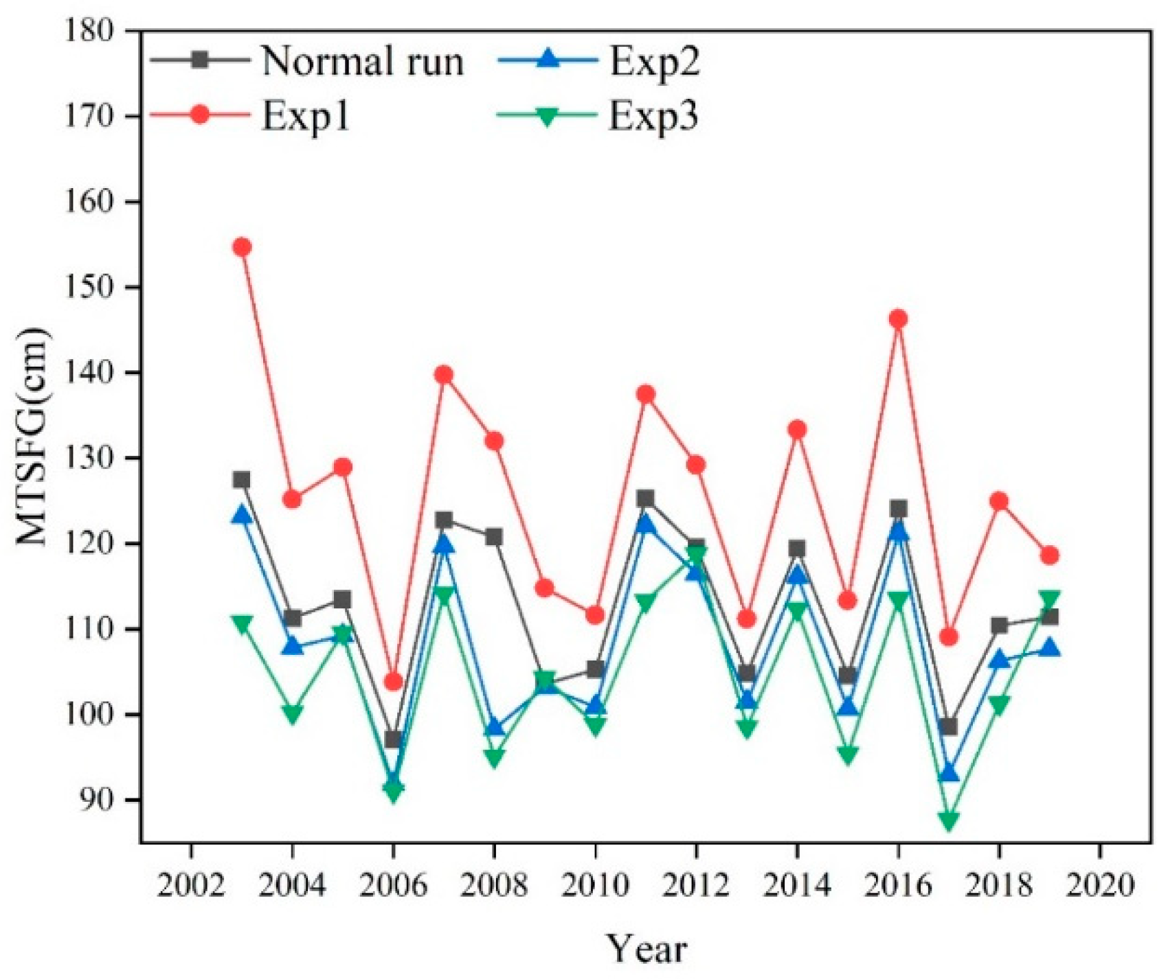
The MTSFG estimated by the different experiments is illustrated in Figure 9 and Figure S3 in the Supplemental Material. The basin-averaged MTSFG estimated in exp1 was significantly larger than that in the normal run, and the MTSFG estimated at the selected stations in exp1 was also larger than the observations (Figure 9 and Figure S3b). This result indicates that Kersten’s scheme overestimated the MTSFG. The basin-averaged MTSFG estimated in exp2 and exp3 were lower than those in the normal run (Figure 9). Exp2 and exp3 also underestimated the MTSFG at the selected stations (Figure S3c,d). This finding illustrates that the uncertainties in the estimation of the mean daily LST using remote sensing can also greatly affect the accuracy in the calculation of the MTSFG.
5. Discussion
5.1. Comparison with Previous Similar Studies
The results of this study were compared with a widely-used frozen soil map proposed by Zou et al. [39]. Figure 10 shows that the area of the permafrost in the map of Zou et al. [39] was significantly larger than that obtained in this study. Table 2 illustrates that the map of Zou et al. [39] incorrectly identified the ground as permafrost at two boreholes (YNG-2 and YNG-3) at which the observed type was seasonally-frozen ground. This result implies that the map of Zou et al. [39] may overestimate the areas of permafrost in the SRYEARS. Zou et al. [39] used the same MODIS product as that used in this study. However, as illustrated in Section 4.5, the uncertainties in the estimation of the mean daily LST can significant affect the mapping of the frozen soil. Therefore, the differences between our results and those of Zou et al. [39] may be related to the different regression coefficients adopted for the estimation of the mean daily LST using the MODIS data. The regression coefficients adopted by Zou et al. [39] were obtained using the MODIS product and the observations from 2012 at three stations (Wudaoliang, Tanggula and Xidaitan), which are located outside the SRYEARS. In this study, the regression coefficients were obtained by the MODIS product and observations at nine meteorological stations in the SRYEARS during the period of 2003–2019. Therefore, the regression coefficients used in this study are likely to be more reasonable than those of Zou et al. [39]. In addition, different coefficients in the cold and warm seasons were adopted in this study in order to represent the seasonal variations of the diurnal cycle of the LST, which further improved the accuracy of the estimation of the spatial distribution of the frozen soil, as mentioned in Section 4.5.
The results of this study indicate that the MTSFG in the SRYEARS decreased by 3.66 cm/10 years from 2003 to 2019, and this finding is consistent with the results of Wang et al. [20], which estimated a decreasing rate of 3.47 cm/10 years for the MTSFG over the SRYEARS in the period from 1965 to 2014 using spatial interpolated air temperature. The decreasing rate of the MTSFG estimated in this study is lower than that reported by Qin et al. [30], which estimated a decline of 12 cm/10 years for the MTSFG over the SRYEARS in the period from 1981 to 2015 using a physical hydrological model. Qin et al. [30] found an abrupt increase in the air temperature around the year 2002 in the period from 1981 to 2015, and a relatively slow increase in the air temperature after 2002. This pattern implies that the different results in the estimation of the change rate of the MTSFG between our study and Qin et al. [30] may be related to the different study periods. On the other hand, the area of permafrost in the period from 2001 to 2010 estimated by Qin et al. [30] was much lower than that of this study (Figure 2), and it was also less than that estimated by Zou et al. [39]. These results suggest that Qin et al. [30] overestimated the trend of frozen soil degradation, and that the result of this study is more reliable.
As mentioned in Section 3.1, most previous studies assumed that the arithmetic average of the daytime and nighttime remote sensing observed LST can represent the mean daily LST [40]. This assumption entails large uncertainties for the mapping of the frozen soil because of its ignoring the nonlinear diurnal cycle of the LST, which was reported in a recent review literature by Ran et al. [35]. Ouyang et al. [41] used piecewise functions to fit the diurnal variations of the LST. However, this method required hourly in-situ observations for LST in order to estimate the parameters of the functions, which were difficult to extend for application in large river basins where hourly observations were usually absent. Hu et al. [42] utilized the adaptive network-based fuzzy inference model for the estimation of the mean daily LST, which required a complex numerical algorithm and in-situ observations for the training of the model. Compared with these two previous studies, the method proposed in this study seems to be simpler, and it is efficient for application at a large catchment scale.
5.2. Uncertainties and Limitations of this Study
We performed an uncertainty analysis of the MTSFG estimation at the selected stations using a Monte Carlo method, and 10,000 random samples of each coefficient in Equations (1) and (2) were generated. Figure S4 in the Supplement Material shows that most of the observations were located within the uncertainty band of our simulation. The variations of the upper and lower limit of the uncertainty band were generally consistent with the MTSFG estimated in the normal run and the observations. The result of the normal run was located in the center of the uncertainty band. These results illustrate that the changes in the MTSFG estimated in this study are reliable. They also indicate that the errors in the estimation of the daily mean LST using remote sensing caused evident uncertainties in the calculation of the MTSFG, which was consistent with the findings of the sensitivity analysis mentioned in Section 4.5.
The spatial scale of the MODIS data is 1 km, which restricts its ability to describe the detail in the topography effect on LST. Therefore, the development of high resolution images of the LST is necessary in future studies. Frozen soil is essentially a subsurface phenomenon, whereas LST is limited to monitoring the land surface. Therefore, knowledge of soils is required to simulate the changes in the frozen soil. In this study, the data describing the soil properties were mainly derived from the database developed by Dai et al. [34] and the HWSD. The uncertainties of these databases may influence the accuracy of the results in this study. An expansion of the in-situ sampling of the soil properties is required in order to improve the current soil database in the QTP in the future. In this study, the liquid soil moisture was estimated using the precipitation index estimated by some functions. However, the parameters of the functions were calibrated using the CSMDA soil moisture data. However, uncertainties in describing the spatial heterogeneity of soil moisture in the SRYEARS exist in this soil moisture product based on remote sensing. More accurate soil moisture data in the QTP, particularly data for the soil moisture in the deep layers, are required in the future in order to improve the accuracy of the current method. The simulation of the permafrost using mathematical models combining the remote sensing data is another future work, and the better integration of the in-situ measurements, multi-source remote sensing data and models are also expected to improve the mapping and monitoring of the changes in the frozen soil.
6. Conclusions
In this study, we proposed an approach using MODIS LST products to estimate the spatial distribution of and changes in frozen soil. Based on the TTOP model and the Stefan equation, the changes in the distribution of the permafrost, MTSFG, and ALT in the SRYEARS from 2003 to 2019 were analyzed, and the following conclusions were reached:
- (1)
- A multiple linear regression model with different coefficients in the cold season and warm season was developed, and it showed excellent aptitude for the estimation of the mean daily LST. Comparisons with the in-situ observations indicate that the method proposed in this study can accurately estimate the spatial distribution of permafrost and the changes in the MTSFG using the remote sensing LST data.
- (2)
- The results of the TTOP model suggest that about 4.82% of the permafrost degraded to seasonally-frozen ground in the period from 2003 to 2019 in the SRYEARS. As estimated by the Stefan formula, the basin-averaged MTSFG decreased at a rate of 3.66 cm/10 years in the period from 2003 to 2019, and the basin-averaged ALT of permafrost increased at a rate of 5.46 cm/10 years.
- (3)
- The uncertainties in the estimation of the mean daily LST and the soil’s thermal conductivity are likely to have significant effects on the accuracy of the estimation of the spatial distribution of the permafrost and the MTSFG. The integration of more in-situ measurements, multi-source remote sensing data and models are required in future studies in order to improve the understanding of the frozen soil changes at the catchment scale.
Due to its efficiency, the approach proposed in this study can be applied for the investigation of the frozen soil changes in other large catchments in cold regions with scarce field observations.
Supplementary Materials
The following are available online at https://www.mdpi.com/2072-4292/13/2/180/s1. Figure S1: Spatial distribution of the (a) maximum thickness of seasonally-frozen ground (MTSFG) and (b) active layer thickness (ALT) of permafrost during the period of 2003–2019. Note: The MTSFG is determined within the distribution of the seasonally-frozen ground from 2003 to 2010; the ALT is determined within the distribution of the permafrost from 2011 to 2019. Figure S2: Enlarged map of the distribution of frozen soil in the period from 2003–2014 in the SRYEARS: (a) the normal run; (b) exp1; (c) exp2 and (d) exp3. Figure S3: MTSFG estimated by remote sensing against observations at nine meteorological stations: (a) the normal run; (b) exp1; (c) exp2 and (d) exp3. Figure S4: Comparison of the MTSFG estimated by remote sensing and its uncertainty band with observations at nine meteorological stations. The region filled by the blue color is the uncertainty band of the estimated MTSFG, with a 95% confidence level. Table S1: Validation of the mean daily LST estimated by the MODIS product. Table S2: Comparison of the mean value of the observed and remote sensing estimated annual MTSFG at nine meteorological stations.
Author Contributions
H.C. finished most of the works on the data treatment and modeling; B.G. provided the method for the model’s development, and designed the framework of this study; T.G. finished part of the works on the data treatment; H.C. wrote the manuscript; B.G. and B.W. modified the manuscript. All authors have read and agreed to the published version of the manuscript.
Funding
This research was funded by the National Natural Science Foundation of China (project no. 41630856) and the Grand Special of High resolution On Earth Observation: Application demonstration system of high resolution remote sensing and transportation (Grant No: 07-Y30B03-9001-19/21).
Institutional Review Board Statement
Not applicable.
Informed Consent Statement
Not applicable.
Data Availability Statement
Publicly available datasets were used in this study. This data can be found here: The MODIS LST data is provided by the National Aeronautics and Space Administration (website https://ladsweb.modaps.eosdis.nasa.gov/). The observed meteorological data, land surface temperature data and the frozen depth data are provided by the China Meteorological Administration (website http://data.cma.cn).The DEM data is provided by the International Centre for Tropical Agriculture (website http://srtm.csi.cgiar.org/SELECTION/inputCoord.asp).The soil property data is obtained from the website of the National Tibetan Plateau Data Center (website http://data.tpdc.ac.cn). The 0–100 cm depth soil moisture data is provided by the China Soil Moisture Dataset from Microwave Data Assimilation (website http://en.tpedatabase.cn).
Acknowledgments
The soil suborders data in the Qinghai–Tibet Plateau was provided by Li et al. [38]. We thank Lin Zhao from School of Geographic Sciences in Nanjing University of Information Science and Technology, and Defu Zou from the Institute of Tibetan Plateau Research, Chinese Academy of Science for their help with the data collection. We also wish to thank to the three anonymous reviewers for their constructive and detailed comments.
Conflicts of Interest
The authors declare that there is no conflict of interest with the China Highway Engineering Consultants Corporation.
Abbreviations
The following main abbreviations are used in this manuscript:
| LST | land surface temperature |
| GST | Ground surface temperature |
| MODIS | moderate-resolution imaging spectroradiometer |
| MTSFG | maximum thickness of seasonally-frozen ground(cm) |
| ALT | active layer thickness(cm) |
| SRYEARS | source region of the Yellow River |
| QTP | Qinghai–Tibetan Plateau |
| TTOP | Temperature at the Top of Permafrost |
References
- Woo, M.K. Permafrost Hydrology; Springer: Berlin/Heidelberg, Germany, 2012; pp. 5–6. [Google Scholar]
- Lawrence, D.M.; Koven, C.D.; Swenson, S.C.; Riley, W.J.; Slater, A.G. Permafrost thaw and resulting soil moisture changes regulate projected high-latitude CO2 and CH4 emissions. Environ. Res. Lett. 2015, 10, 9. [Google Scholar] [CrossRef] [Green Version]
- Hayashi, M. The cold vadose zone: Hydrological and ecological significance of frozen-soil processes. Vadose Zone J. 2014, 13, 1. [Google Scholar] [CrossRef]
- Jin, X.Y.; Jin, H.J.; Iwahana, G.; Marchenko, S.S.; Liang, S.H. Impacts of climate-induced permafrost degradation on vegetation: A review. Adv. Clim. Chang. Res. 2020. [Google Scholar] [CrossRef]
- Walter, W.; Van Beek, L.P.H.; Bierkens, M.F.P. Climate Change Will Affect the Asian Water Towers. Science 2010, 328, 1382–1385. [Google Scholar] [CrossRef]
- Cuo, L.; Zhang, Y.; Bohn, T.J.; Zhao, L.; Li, J.; Liu, Q.; Zhou, B. Frozen soil degradation and its effects on surface hydrology in the northern Tibetan Plateau. J. Geophys. Res. Atmos. 2015, 120, 8276–8298. [Google Scholar] [CrossRef] [Green Version]
- Qin, Y.; Lei, H.; Yang, D.W.; Gao, B.; Wang, Y.H.; Cong, Z.T.; Fan, W.J. Long-term change in the depth of seasonally frozen ground and its ecohydrological impacts in the Qilian Mountains, northeastern Tibetan Plateau. J. Hydrol. 2016, 542, 204–221. [Google Scholar] [CrossRef]
- Gao, B.; Yang, D.W.; Qin, Y.; Wang, Y.H.; Li, H.Y.; Zhang, Y.L.; Zhang, T.J. Change in frozen soils and its effect on regional hydrology, upper Heihe Basin, northeastern Qinghai-Tibetan Plateau. Cryosphere 2018, 12, 657–673. [Google Scholar] [CrossRef] [Green Version]
- Niu, L.; Ye, B.S.; Li, J.; Sheng, Y. Effect of permafrost degradation on hydrological processes in typical basins with various permafrost coverage in Western China. Sci. China Earth Sci. 2011, 54, 615–624. [Google Scholar] [CrossRef]
- Zhang, W.J.; Yi, Y.H.; Kimball, J.S.; Kim, Y.; Song, K.C. Climatic controls on spring onset of the Tibetan Plateau Grasslands from 1982 to 2008. Remote Sens. 2015, 7, 16607–16622. [Google Scholar] [CrossRef] [Green Version]
- Gao, B.; Li, J.; Wang, X.S. Impact of frozen soil changes on vegetation phenology in the source region of the Yellow River from 2003 to 2015. Theor. Appl. Climatol. 2020, 141, 1219–1234. [Google Scholar] [CrossRef]
- Chen, S.Y.; Liu, W.J.; Qin, X.; Liu, Y.S.; Zhang, T.Z.; Chen, K.L.; Hu, F.Z.; Ren, J.W.; Qin, D.H. Response characteristics of vegetation and soil environment to permafrost degradation in the upstream regions of the Shule River Basin. Environ. Res. Lett. 2012, 7, 189–190. [Google Scholar] [CrossRef] [Green Version]
- Wania, R. Integrating peatlands and permafrost into a dynamic global vegetation model: 1. Evaluation and sensitivity of physical land surface processes. Glob. Biogeochem. Cycle 2009, 23, 3. [Google Scholar] [CrossRef] [Green Version]
- Guo, D.L.; Wang, H. Simulation of permafrost and seasonally frozen ground conditions on the Tibetan Plateau, 1981–2010. J. Geophys. Res. Atmos. 2013, 118, 5216–5230. [Google Scholar] [CrossRef]
- Wang, T.H.; Yang, D.W.; Fang, B.J.; Yang, W.C.; Qin, Y.; Wang, Y.H. Data-driven mapping of the spatial distribution and potential changes of frozen ground over the Tibetan Plateau. Sci. Total Environ. 2018, 649, 515–525. [Google Scholar] [CrossRef] [PubMed]
- Ran, Y.H.; Li, X.; Cheng, G.D.; Nan, Z.T.; Che, J.X.; Sheng, Y.; Wu, Q.B.; Jin, H.J.; Luo, D.L.; Tang, Z.G.; et al. Mapping the permafrost stability on the Tibetan Plateau for 2005–2015. Sci. China Earth Sci. 2020, 63, 1–18. [Google Scholar] [CrossRef]
- Smith, M.W.; Riseborough, D.W. Permafrost monitoring and detection of climate change. Permafr. Periglac. Process. 1996, 7, 301–309. [Google Scholar] [CrossRef]
- Stefan, J. Ueber die Theorie der Eisbildung, insbesondere über die Eisbildung im Polarmeere. Ann. Phys. Berlin. 1891, 278, 269–286. [Google Scholar] [CrossRef] [Green Version]
- Peng, X.Q.; Frauenfeld, O.; Zhang, T.J.; Wang, K.; Cao, B.; Zhong, X.Y.; Hang, S.; Mu, C.C. Response of seasonal soil freeze depth to climate change across China. Cryosphere 2017, 11, 1059–1073. [Google Scholar] [CrossRef] [Green Version]
- Wang, T.H.; Yang, D.W.; Qin, Y.; Wang, Y.H.; Chen, Y.; Gao, B.; Yang, H.B. Historical and future changes of frozen ground in the upper Yellow River Basin. Glob. Planet. Chang. 2018, 162, 199–211. [Google Scholar] [CrossRef]
- Riseborough, D.; Shiklomanov, N.; Etzelmüller, B.; Gruber, S.; Marchenko, S. Recent advances in permafrost modelling. Permafr. Periglac. Process. 2008, 19, 137–156. [Google Scholar] [CrossRef]
- Wang, C.H.; Jin, S.L.; Wu, Z.Y.; Cui, Y. Evaluation and Application of the Estimation Methods of Frozen (Thawing) Depth over China. Adv. Earth Sci. 2009, 24, 132–141. (In Chinese) [Google Scholar] [CrossRef]
- Zheng, G.H.; Yang, Y.T.; Yang, D.W.; Dafflon, B.; Lei, H.M.; Yang, H.B. Satellite-based simulation of soil freezing/thawing processes in the northeast Tibetan Plateau. Remote Sens. Environ. 2019, 231, 111269. [Google Scholar] [CrossRef]
- Langer, M.; Westermann, S.; Boike, J. Spatial and temporal variations of summer surface temperatures of wet polygonal tundra in Siberia-implications for MODIS LST based permafrost monitoring. Remote Sens. Environ. 2010, 114, 2059–2069. [Google Scholar] [CrossRef]
- Yang, Y.K.; Li, H.; Sun, L.; Du, Y.M.; Cao, B.; Liu, Q.H.; Zhu, J.S. Land surface temperature and emissivity separation from Gaofen-5 multispectral imager data. J. Remote Sens. 2019, 23, 1090–1104. (In Chinese) [Google Scholar] [CrossRef]
- Zou, D.F.; Zhao, L.; Wu, T.H.; Wu, X.D.; Pang, Q.Q.; Qiao, Y.P.; Wang, Z.W. Assessing the applicability of MODIS land surface temperature products in continuous permafrost regions in the central Tibetan Plateau. Glacier Permafrost. 2015, 37, 308–317. (In Chinese) [Google Scholar] [CrossRef]
- Obu, J.; Westermann, S.; Bartsch, A.; Berdnikov, N.; Christiansen, H.; Avirmed, D.; Delaloye, R.; Elberling, B.; Etzelmüller, B.; Kholodov, A.; et al. Northern Hemisphere permafrost map based on TTOP modelling for 2000–2016 at 1 km2 scale. Earth Sci. Rev. 2019, 193, 299–316. [Google Scholar] [CrossRef]
- Wang, R.; Dong, Z.B.; Zhou, Z.C. Effect of decreasing soil frozen depth on vegetation growth in the source region of the Yellow River for 1982–2015. Theor. Appl. Climatol. 2020, 140, 3–4. [Google Scholar] [CrossRef]
- Hu, Y.R.; Maskey, S.; Zhao, U.L. Streamflow trends and climate linkages in the source region of the Yellow River, China. Hydrol. Process. 2011, 25, 3399–3411. [Google Scholar] [CrossRef]
- Qin, Y.; Yang, D.W.; Gao, B.; Wang, T.H.; Chen, J.; Chen, Y.; Wang, Y.; Zheng, G. Impacts of climate warming on the frozen ground and eco-hydrology in the Yellow River source region, China. Sci. Total Environ 2017, 605–606, 830–841. [Google Scholar] [CrossRef] [Green Version]
- Shen, Y.; Xiong, A.Y. Validation and comparison of a new gauge-based precipitation analysis over mainland China. Int. J. Climatol. 2016, 36, 252–265. [Google Scholar] [CrossRef]
- Luo, D.L.; Jin, H.J.; Lin, L.; He, R.X.; Yang, S.Z.; Chang, X.L. New Progress on Permafrost Temperature and Thickness in the Source Area of the Huanghe River. Sci. Geogr. Sin. 2012, 32, 898–904. (In Chinese) [Google Scholar] [CrossRef]
- Food and Agriculture Organization of the United Nations(FAO); International Institute for Applied Systems Analysis. China Soil Map Based Harmonized World Soil Database (HWSD) (v1.1) (2009); National Tibetan Plateau Data Center: Beijing, China, 2019. [Google Scholar]
- Dai, Y.J.; Shang, G.W.; Duan, Q.Y.; Liu, B.Y.; Fu, S.H.; Niu, G.Y. Development of a China Dataset of Soil Hydraulic Parameters Using Pedotransfer Functions for Land Surface Modeling. J. Hydrometeorol. 2013, 14, 869–887. [Google Scholar] [CrossRef] [Green Version]
- Ran, Y.; Li, X. Progress, challenges and opportunities of permafrost mapping in China. Adv. Earth Sci. 2019, 34, 1015–1027. (In Chinese) [Google Scholar]
- Farouki, O.T. The thermal properties of soils in cold regions. Cold Reg. Sci. Technol. 1981, 5, 67–75. [Google Scholar] [CrossRef]
- Kersten, M.S. Laboratory research for the determination of the thermal properties of soils. J. Neurophysiol. 1948, 45, 667–697. [Google Scholar] [CrossRef]
- Li, W.P.; Zhao, L.; Wu, X.D.; Zhao, Y.H.; Fang, H.B.; Shi, W. Distribution of soils and landform relationships in the permafrost regions of Qinghai-Xizang (Tibetan) Plateau. Chin. Sci. Bull. 2015, 60, 2216–2226. (In Chinese) [Google Scholar] [CrossRef]
- Zou, D.F.; Zhao, L.; Sheng, Y.; Chen, J.; Hu, G.J.; Wu, T.H.; Pang, Q.; Wang, W. A new map of permafrost distribution on the Tibetan Plateau. Cryosphere 2017, 11, 1–28. [Google Scholar] [CrossRef] [Green Version]
- Ran, Y.H.; Li, X.; Jin, R.; Guo, J.W. Remote sensing of the mean annual surface temperature and surface frost number for mapping permafrost in China. Arct. Antarct. Alp. Res. 2015, 47, 255–265. [Google Scholar] [CrossRef] [Green Version]
- Ouyang, B.; Che, T.; Dai, L.Y.; Wang, Z.Y. Estimating Mean Daily Surface Temperature over the Tibetan Plateau Based on MODIS LST Products. J. Glaciol. Geocryol. 2012, 34, 296–303. (In Chinese) [Google Scholar]
- Hu, J.N.; Zhao, S.P.; Nan, Z.T.; Wu, X.B.; Sun, X.H.; Cheng, G.D. An effective approach for mapping permafrost in a large area using subregion maps and satellite data. Permafr. Periglac. Process. 2020, 31, 548–560. [Google Scholar] [CrossRef]
Figure 1.
Study area and the locations of the meteorological stations.

Figure 2.
Distribution of the frozen soil estimated by remote sensing in the period from 2005 to 2014, and the locations of the 10 boreholes [32].
Figure 2.
Distribution of the frozen soil estimated by remote sensing in the period from 2005 to 2014, and the locations of the 10 boreholes [32].

Figure 3.
Variables estimated by remote sensing against the observations at nine meteorological stations: (a) the mean daily LST, (b) the MTSFG.
Figure 3.
Variables estimated by remote sensing against the observations at nine meteorological stations: (a) the mean daily LST, (b) the MTSFG.

Figure 4.
Comparison of the temporal variations of the observed and remote-sensing–estimated MTSFG at the: (a) Xinghai station, (b) Maduo station, (c) Maqin station, (d) Dari station, (e) Henan station, (f) Jiuzhi station, (g) Maqu station, (h) Zogie station, and (i) Hongyuan station.
Figure 4.
Comparison of the temporal variations of the observed and remote-sensing–estimated MTSFG at the: (a) Xinghai station, (b) Maduo station, (c) Maqin station, (d) Dari station, (e) Henan station, (f) Jiuzhi station, (g) Maqu station, (h) Zogie station, and (i) Hongyuan station.

Figure 5.
Changes in the distribution of frozen soil types from Period 1 (2003–2010) to Period 2 (2011–2019). PF means permafrost and SFG means seasonally-frozen ground.
Figure 5.
Changes in the distribution of frozen soil types from Period 1 (2003–2010) to Period 2 (2011–2019). PF means permafrost and SFG means seasonally-frozen ground.

Figure 6.
Changes in the basin-averaged (a) MTSFG and (b) ALT of the permafrost estimated by remote sensing. The observed mean annual air temperature in the period from 2003 to 2019 are also shown in the figure.
Figure 6.
Changes in the basin-averaged (a) MTSFG and (b) ALT of the permafrost estimated by remote sensing. The observed mean annual air temperature in the period from 2003 to 2019 are also shown in the figure.

Figure 7.
Spatial distribution of the change rate of the (a) annual maximum thickness of the seasonally-frozen ground (MTSFG) and (b) the annual active layer thickness (ALT) of the permafrost in the period from 2003 to 2019.
Figure 7.
Spatial distribution of the change rate of the (a) annual maximum thickness of the seasonally-frozen ground (MTSFG) and (b) the annual active layer thickness (ALT) of the permafrost in the period from 2003 to 2019.

Figure 8.
Map of the distribution of the frozen soil in the period from 2005 to 2014 in the SRYEARS: (a) the normal run, (b) exp1, (c) exp2, and (d) exp3. Note: PF = permafrost and SFG = seasonally-frozen ground.
Figure 8.
Map of the distribution of the frozen soil in the period from 2005 to 2014 in the SRYEARS: (a) the normal run, (b) exp1, (c) exp2, and (d) exp3. Note: PF = permafrost and SFG = seasonally-frozen ground.

Figure 9.
Changes in the basin-averaged MTSFG in the period from 2003 to 2019, estimated by remote sensing in the normal run, exp1, exp2 and exp3.
Figure 9.
Changes in the basin-averaged MTSFG in the period from 2003 to 2019, estimated by remote sensing in the normal run, exp1, exp2 and exp3.

Figure 10.
Map showing the distribution of the permafrost in the SRYEARS: (a) the results of this study, (b) the map from Zou et al. [39].
Figure 10.
Map showing the distribution of the permafrost in the SRYEARS: (a) the results of this study, (b) the map from Zou et al. [39].


Table 1.
Description of the observed data at nine national meteorological stations.
| Station Name | Elevation(m) | Latitude | Longitude | Landcover | Starting and Ending Years of Observation | ||
|---|---|---|---|---|---|---|---|
| MTSFG | LST | Air Temperature & Precipitation | |||||
| Xinghai | 3323.2 | 35°35′ | 99°59′ | Steppe | 2003–2015 | 2003–2015 | 2003–2019 |
| Maduo | 4272.3 | 34°55′ | 98°13′ | Steppe | 2003–2015 | 2003–2015 | 2003–2019 |
| Maqin | 3719.0 | 34°29′ | 100°14′ | Meadow | 2003–2015 | 2003–2015 | 2003–2019 |
| Dari | 3967.5 | 33°45′ | 99°39′ | Meadow | 2003–2015 | 2003–2015 | 2003–2019 |
| Henan | 3500.0 | 34°44′ | 101°36′ | Meadow | 2003–2015 | 2003–2015 | 2003–2019 |
| Jiuzhi | 3628.5 | 33°26′ | 101°29′ | Meadow | 2003–2015 | 2003–2015 | 2003–2019 |
| Maqu | 3471.4 | 34°00′ | 102°05′ | Steppe | 2007–2015 | 2003–2015 | 2003–2019 |
| Zoige | 3441.4 | 33°35′ | 102°58′ | Meadow | 2003–2015 | 2003–2015 | 2003–2019 |
| Hong-yuan | 3491.6 | 32°48′ | 102°33′ | Meadow | 2003–2015 | 2003–2015 | 2003–2019 |
Table 2.
Validation of the frozen soil types estimated by the TTOP model at 10 boreholes.
| Station Name | Latitude | Longitude | Elevation(m) | Drilling Time | Observed Type | Estimated Type in this Study | Estimated Type by Zou et al. [39] |
|---|---|---|---|---|---|---|---|
| CLP-1 | 34.25 | 97.85 | 4727 | 2010/8 | PF | PF | PF |
| CLP-2 | 34.25 | 97.85 | 4723 | 2010/8–9 | PF | PF | PF |
| CLP-3 | 34.27 | 97.87 | 4663 | 2010/8 | PF | PF | PF |
| CLP-4 | 34.32 | 97.9 | 4564 | 2010/8 | PF | PF | PF |
| YNG-1 | 34.4 | 97.95 | 4452 | 2010/8 | PF | PF | PF |
| YNG-2 | 34.43 | 97.93 | 4395 | 2010/8 | SFG | SFG | PF |
| YNG-3 | 34.5 | 97.97 | 4333 | 2010/8 | SFG | SFG | PF |
| XXH-1 | 34.65 | 98.43 | 4231 | 2010/8 | SFG | SFG | SFG |
| MDB | 34.85 | 98.55 | 4225 | 2010/9 | PF | PF | PF |
| K445 | 34.97 | 98.55 | 4288 | 2010/9 | PF | PF | PF |
Note: PF means permafrost and SFG means seasonally-frozen ground. The boreholes drilled in 2010 were compared with the results based on the mean values of TTOP in the period of 2005–2014.
Table 3.
Comparison of the parameterization of the frozen soil mapping in the normal run, exp1, exp2, and exp3.
Table 3.
Comparison of the parameterization of the frozen soil mapping in the normal run, exp1, exp2, and exp3.
| The Scheme For Thermal Conductivity Estimation | Regression Coefficients for the Estimation of the Mean Daily LST | ||||||
|---|---|---|---|---|---|---|---|
| a1 | a2 | a3 | a4 | b | |||
| Normal run | Johansen’s scheme | Warm season | 0.154 | 0.274 | 0.096 | 0.428 | 4.775 |
| Cold season | 0.109 | 0.229 | 0.104 | 0.341 | 7.802 | ||
| Exp1 | Kersten’s scheme | Warm season | 0.154 | 0.274 | 0.096 | 0.428 | 4.775 |
| Cold season | 0.109 | 0.229 | 0.104 | 0.341 | 7.802 | ||
| Exp2 | Johansen’s scheme | - | 0.170 | 0.307 | 0.111 | 0.442 | 5.564 |
| Exp3 | Johansen’s scheme | - | 0.25 | 0.25 | 0.25 | 0.25 | 0 |
Note: LSTmean = a1 × LSTmodd+a2 × LSTmodn + a3 × LSTmydd + a4 × LSTmydn + b; modd means Terra daytime, modn means Terra nighttime, mydd means Aqua daytime, and mydn means Aqua nighttime.
Table 4.
Frozen soil types estimated at 10 boreholes in the normal run, exp1, exp2, and exp3.
| Station Name | Observed | Normal Run | Exp1 | Exp2 | Exp3 |
|---|---|---|---|---|---|
| CLP-1 | PF | PF | PF | PF | PF |
| CLP-2 | PF | PF | PF | PF | PF |
| CLP-3 | PF | PF | PF | PF | PF |
| CLP-4 | PF | PF | PF | PF | PF |
| YNG-1 | PF | PF | SFG | PF | PF |
| YNG-2 | SFG | SFG | SFG | PF | PF |
| YNG-3 | SFG | SFG | SFG | SFG | SFG |
| XXH-1 | SFG | SFG | SFG | SFG | SFG |
| MDB | PF | PF | PF | PF | PF |
| K445 | PF | PF | PF | PF | PF |
Note: PF = permafrost and SFG = seasonally-frozen ground.
Publisher’s Note: MDPI stays neutral with regard to jurisdictional claims in published maps and institutional affiliations. |
© 2021 by the authors. Licensee MDPI, Basel, Switzerland. This article is an open access article distributed under the terms and conditions of the Creative Commons Attribution (CC BY) license (http://creativecommons.org/licenses/by/4.0/).
Share and Cite
MDPI and ACS Style
Cao, H.; Gao, B.; Gong, T.; Wang, B. Analyzing Changes in Frozen Soil in the Source Region of the Yellow River Using the MODIS Land Surface Temperature Products. Remote Sens. 2021, 13, 180. https://doi.org/10.3390/rs13020180
AMA Style
Cao H, Gao B, Gong T, Wang B. Analyzing Changes in Frozen Soil in the Source Region of the Yellow River Using the MODIS Land Surface Temperature Products. Remote Sensing. 2021; 13(2):180. https://doi.org/10.3390/rs13020180
Chicago/Turabian StyleCao, Huiyu, Bing Gao, Tingting Gong, and Bo Wang. 2021. "Analyzing Changes in Frozen Soil in the Source Region of the Yellow River Using the MODIS Land Surface Temperature Products" Remote Sensing 13, no. 2: 180. https://doi.org/10.3390/rs13020180
Note that from the first issue of 2016, this journal uses article numbers instead of page numbers. See further details here.