Article

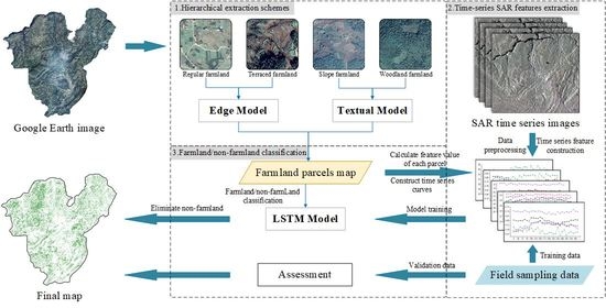
Farmland Parcel Mapping in Mountain Areas Using Time-Series SAR Data and VHR Optical Images

1
University of Chinese Academy of Sciences, Beijing 100049, China
2
State Key Laboratory of Remote Sensing Science, Aerospace Information Research Institute, Chinese Academy of Sciences, Beijing 100101, China
3
Ant Group, Hangzhou 310013, China
4
School of Geographical Sciences, Guangzhou University, Guangzhou 510006, China
5
School of Earth Science and Engineering, Hohai University, Nanjing 211100, China
6
Institute of Agricultural Resources and Agricultural Regionalization, Chinese Academy of Agricultural Sciences, Beijing 100081, China
7
National Engineering Research Center for Geomatics, Aerospace Information Research Institute, Chinese Academy of Sciences, Beijing 100101, China
*
Author to whom correspondence should be addressed.
Remote Sens. 2020, 12(22), 3733; https://doi.org/10.3390/rs12223733
Submission received: 24 September 2020 / Revised: 2 November 2020 / Accepted: 9 November 2020 / Published: 13 November 2020

Abstract

:
Accurate, timely, and reliable farmland mapping is a prerequisite for agricultural management and environmental assessment in mountainous areas. However, in these areas, high spatial heterogeneity and diversified planting structures together generate various small farmland parcels with irregular shapes that are difficult to accurately delineate. In addition, the absence of optical data caused by the cloudy and rainy climate impedes the use of time-series optical data to distinguish farmland from other land use types. Automatic delineation of farmland parcels in mountain areas is still a very difficult task. This paper proposes an innovative precise farmland parcel extraction approach supported by very high resolution(VHR) optical image and time series synthetic aperture radar(SAR) data. Firstly, Google satellite imagery with a spatial resolution of 0.55 m was used for delineating the boundaries of ground parcel objects in mountainous areas by a hierarchical extraction scheme. This scheme divides farmland into four types based on the morphological features presented in optical imagery, and designs different extraction models to produce each farmland type, respectively. The potential farmland parcel distribution map is then obtained by the layered recombination of these four farmland types. Subsequently, the time profile of each parcel in this map was constructed by five radar variables from the Sentinel-1A dataset, and the time-series classification method was used to distinguish farmland parcels from other types. An experiment was carried out in the north of Guiyang City, Guizhou Province, Southwest China. The result shows that, the producer’s accuracy of farmland parcels obtained by the hierarchical scheme is increased by 7.39% to 96.38% compared with that without this scheme, and the time-series classification method produces an accuracy of 80.83% to further obtain the final overall accuracy of 96.05% for the farmland parcel maps, showing a good performance. In addition, through visual inspection, this method has a better suppression effect on background noise in mountainous areas, and the extracted farmland parcels are closer to the actual distribution of the ground farmland.

Graphical Abstract

1. Introduction

The spatial distribution information of farmland is essential for promoting agricultural production and policy making, and has been widely used in various agricultural applications, such as yield estimation, ecological environment assessment, and food risk analysis [1,2,3]. In mountainous areas, due to the impact of population, environment, and soil fertility, smallholder farms are the most common form of agriculture and provide food for the majority of the population [4]. The farmland spatial distribution map of smallholder farms plays a critical role in mountainous agricultural management and food security. However, smallholde farmers often cause uncertainties in the use of farmland and varies from year to year because of various factors (such as economic shocks and land use policies) [5]. Therefore, the spatial distribution maps of farmland are not available in most mountainous areas, which seriously hinders the improvement of mountainous agricultural production [4]. The traditional statistical methods of agricultural information that almost rely on field surveys are severely restricted in terms of economic efficiency, representativeness, and reliability. Remote sensing technology can continuously and quickly obtain ground information over large areas at low cost, which provides the possibility of systematically mapping farmland distribution at regional and global scales.
With the popularity of accessible satellite data, many studies have achieved certain results in the use of remote sensing data to extract farmland spatial distribution information [6,7,8,9,10,11]. Moreover, with the increase of the spatial resolution, the basic unit of farmland mapping is also converted from pixel to object [12]. Compared with the pixel-oriented method, the object-oriented method have obvious advantages in extracting ground information from high-resolution remote sensing images [13,14,15]. However, precise farmland spatial distribution mapping in complex scenes is still a quite challenging task, which mainly includes the following two aspects:
  • The high heterogeneity in mountainous areas produces a host of small farmland parcels with irregular shapes. These parcels with multiple crops construct a complex planting structure, which leads to the difficulty of obtaining accurate boundaries of the ground objects.
  • Universal cloud coverage in mountainous areas, caused by rainy and hot weather during the same period, results in the absence of opportune optical data, which makes it hardly to distinguish farmland parcels from other parcel types.
Regarding the first issue, recent remote sensing satellite sensors have provided new possibilities for monitoring small farmland parcels in mountainous areas [16]. For example, the very high resolution (VHR) images, with a spatial resolution of 1 m or finer, can more clearly describe the morphological features of image objects, and easily distinguish the boundaries and textures of farmland parcels, which are hard to obtain from high to medium resolution satellite images. However, the substantial content and complex form of VHR images in mountainous areas also bring a new challenge to the mapping of farmland spatial distribution.
In recent years, deep learning technology has made great progress in the field of computer vision. In particular, the convolutional neural networks (CNNs), with the ability to learn and process a hierarchy of spatial features, have shown a remarkable ability in image classification and semantic segmentation [17,18,19]. Recently, CNNs have been applied to remote sensing tasks, such as land cover/land use(LCLU) classification [20,21,22,23,24,25,26], object detection [27,28,29], and scene classification [30,31]. The CNNs are able to learn high-level abstract features from the raw pixels of satellite images, and achieve remarkable performance in VHR images classification [32]. Various CNN architectures have been investigated for LCLU classification in simple remote sensing scenes. However, for complex scenes, these investigations, which focus on sample optimization or model improvement, always intend to use only one model or method to achieve the extraction of all target image objects in VHR remote sensing images. With the increasing complexity of the model structure adjustment, it also brings a burden to the production of a large number of samples, and the results achieved so far are still relatively limited [33].
To deal with complex scenes, a hierarchical method based on a divided and stratified strategy is introduced into satellite image information extraction. Wu and Li [34] made use of such a strategy for crop acreage estimation in complex agricultural landscapes. Their method significantly improves the estimation accuracy and, at the same time, reduces the field sampling cost. Fenske et al. [35] proposed a 3-level hierarchical classification method to obtain heathland habitats, and their study showed that the hierarchical classification approach can distinguish ambiguous target objects from VHR images in complex landscapes. Haest et al. [36] also found that a hierarchical classification is beneficial to the classification of remote sensing images. Therefore, under the guidance of the divided and stratified strategy, the farmland extraction method is able to obtain precise parcel objects from VHR optical imagery without a host of model improvements and sample making tasks.
Regarding the second issue, it is worth noting that there are many farmland-like parcels that are similar to the visual features of farmland in VHR images (such as idle farmland, wasteland, and grassland). Especially with the hierarchical method, these farmland-like parcels are often extracted as farmland by CNNs. Past studies indicate that most crops exhibit a unique phenological pattern. Therefore, time-series satellite datasets covering the entire growing season of crops can be used to develop features for mapping crop distribution [1]. Nevertheless, for mountainous areas, cloudy and rainy weather leads to a lack of optical data, and it is impossible to collect enough cloud-free optical images to construct the time-series features of crops to remove these farmland-like parcels [37].
Instead of optical sensors, Synthetic Aperture Radar (SAR) is an active imaging technology that transmits and receives electromagnetic waves in the microwave range and can penetrate clouds. With the advantages of all-weather data acquisition, SAR has shown great potential for remote sensing monitoring in cloudy and rainy areas [38,39]. The SAR backscattering intensity is affected by multiple factors such as vegetation structure and ground surface properties, mainly including direct backscattering from the vegetation canopy, ground backscattering weakened by the vegetation canopy, and backscattering from the interaction between vegetation and the ground [40]. In particular, the structure of the vegetation canopy plays an important role in the influence factors of SAR backscattering intensity changes [41]. Therefore, due to the substantial changes in crop canopy structure at different growth stages, SAR time series data shows a great potential to map the farmland distribution [42,43,44]. However, in the mountainous areas, the complex agricultural landscapes, composed of multiple crops where inter-cropping is common, have brought a new challenge to time series classification. The Recurrent Neural Networks (RNNs) [45] are a mature machine learning technology, which has shown good performance in different fields such as speech recognition, signal processing, and natural language processing [46,47,48]. In the remote sensing field, recent studies have shown great potential for crop classification using RNN in satellite image time series [49,50,51]. Unlike convolutional neural networks, RNNs can explicitly manage the temporal data dependencies, and are suitable for mining time series features of multitemporal datasets [52], such as time series SAR data for farmland.
In this paper, we propose a precise farmland parcel extraction method in complex scenes (i.e., mountains of Southwest China) by incorporating VHR optical images and time series SAR data. VHR Google satellite optical imagery with a spatial resolution of 0.55 m was used to delineate the precise parcel object distribution map, and Sentinel-1A (S1A) SAR datasets provided the backscattering features to construct the temporal behaviors of parcel objects to further distinguish farmland parcels from other types. Furthermore, a CNN-based hierarchical extraction scheme was developed for parcel extraction in complex scenes, and an LSTM-based classification method was used to learn time-series SAR features of these parcels. This study is designed to solve a host of difficulties, such as landscape fragmentation, complex planting structures, and cloudy and rainy weather in mountainous areas, and achieved the following objectives:
  • By using CNN technology, a hierarchical extraction scheme based on VHR optical images was developed to obtain an accurate image object distribution map of complex scenes such as mountainous areas.
  • Combined with the LSTM networks, the potential of multiple variables of time-series SAR for farmland parcel identification is fully explored in cloudy and rainy areas.
We conducted an experiment in the north of Guiyang City, Guizhou Province, Southwestern China. This experiment focuses on developing an automatic method for precise farmland parcel mapping in complex landscapes, and the results validate the effectiveness and feasibility of this method.

2. Study Area and Dataset
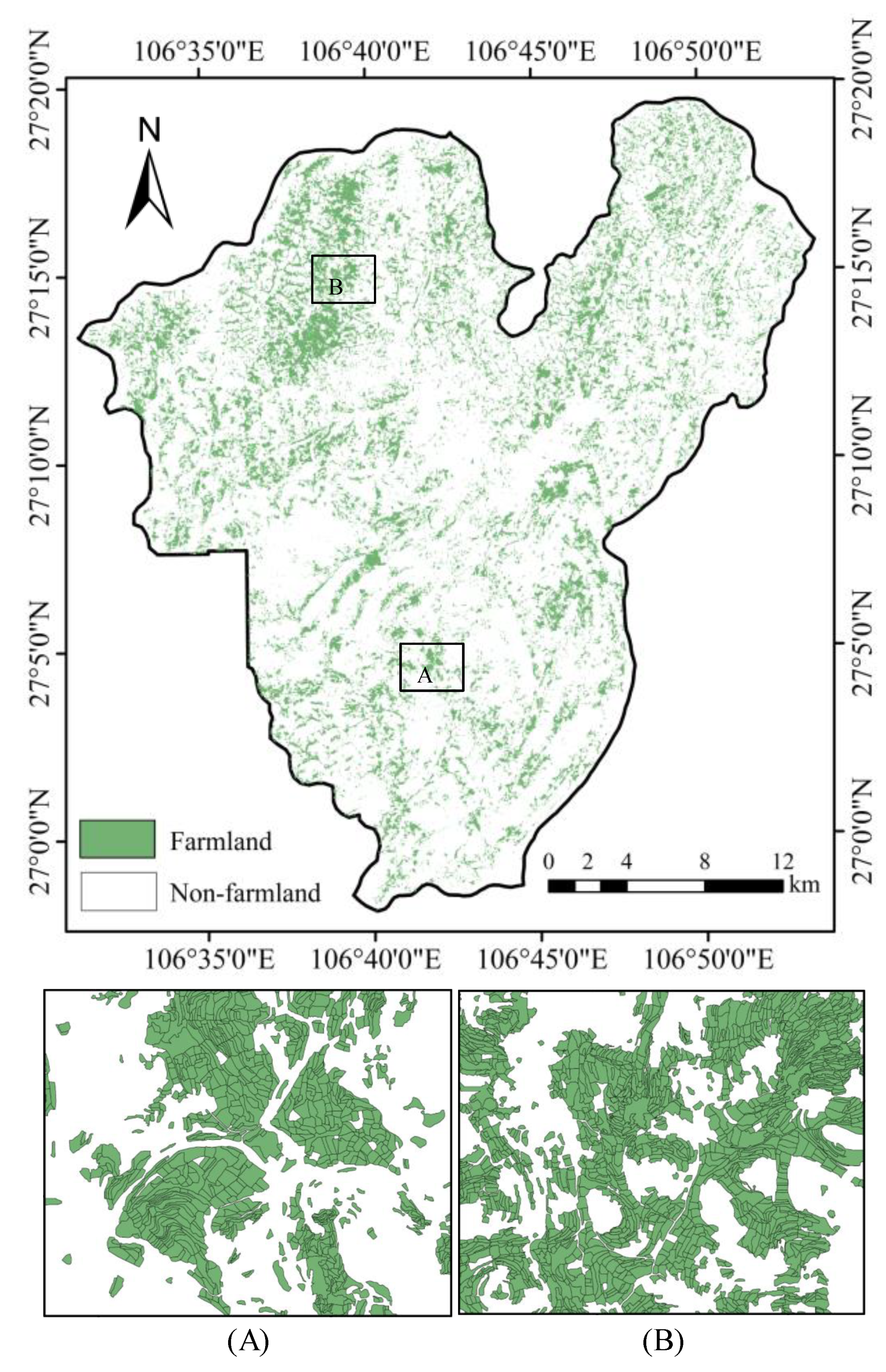
2.1. Study Site

To evaluate the proposed method, a typical karst hilly region in Southwest China was selected as the experimental area. As illustrated in Figure 1, this study area is located in the north of Guiyang City, Guizhou Province, China, with an area of about 794 km 2 (center latitude and longitude is 27 9 59 N, 106 42 24 E). In this region of hilly lands, the terrain is low in the north and high in the south, with an altitude ranging from 600 to 1800 m. This area is mainly covered by farmland, woodland, grassland, buildings, and water, which together constitutes a complex and diverse agricultural landscape. Due to the mild climate, abundant precipitation and great variations in elevation, it is suitable for the growth of various agricultural crops, such as rice, rape, soybeans, and corn, and some scattered farmlands grow various vegetables such as cucumber, pepper, and cabbage. According to local planting practices, corn is planted from April to May and harvested from September to October, while rice and soybean are planted from May to June and harvested from September to October. As the main winter crop in this region, rape is planted from November to October and harvested from April to May. In addition, various vegetables are planted all year round. In this area, cloudy and rainy weather throughout the year made it difficult to obtain sufficient cloudless optical image data. Therefore, how the limited optical data and time series SAR data can be used for farmland mapping in mountainous areas is an urgent problem to be solved.

2.2. Remote Sensing Data

It is hard to obtain fully covered VHR optical images for a cloudy and rainy study area. Therefore, in this study, Google satellite images with a spatial resolution of 0.55 m was downloaded and employed for delineating the boundaries of ground objects (Figure 1). This image has three spectral bands that provide detailed spatial and spectral information and clearly describe the land cover information.
S1A SAR of European Space Agency (ESA) provides C-band radar images at a center frequency of 5.405 GHz. The interferometric wide swath (IW) is the default acquisition mode over land, with an available dual polarization (VV + VH and HH + HV) operation mode. The geometric resolution is 5 m by 20 m with a large swath width of 250 km. The dataset used in this study consists of a time series of 30 S1A images (Table 1) between January 2019 and December 2019, with a time interval of 12 days. All the radar imagery we used was acquired in TOPS mode with dual-polarization (VV + VH) from the Copernicus Open Access Hub as Single Look Complex products collected in ascending passes.

2.3. Field Sampling Data
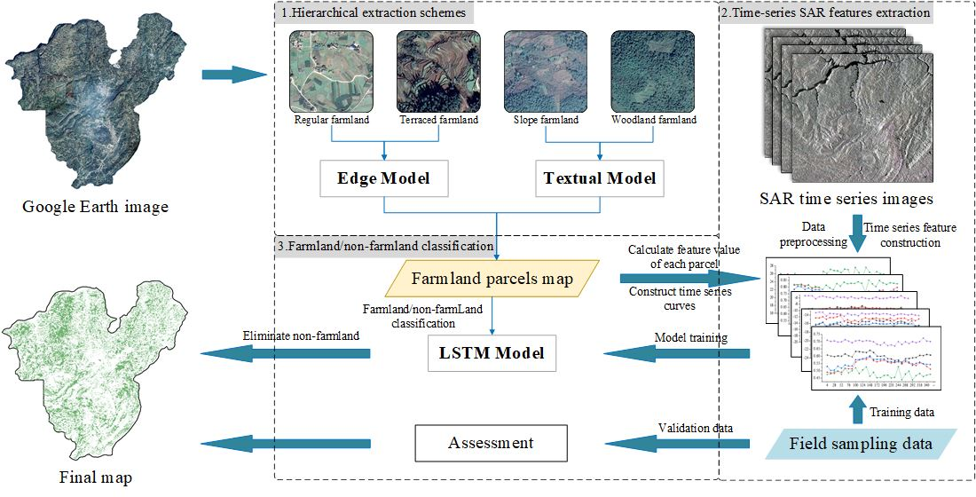
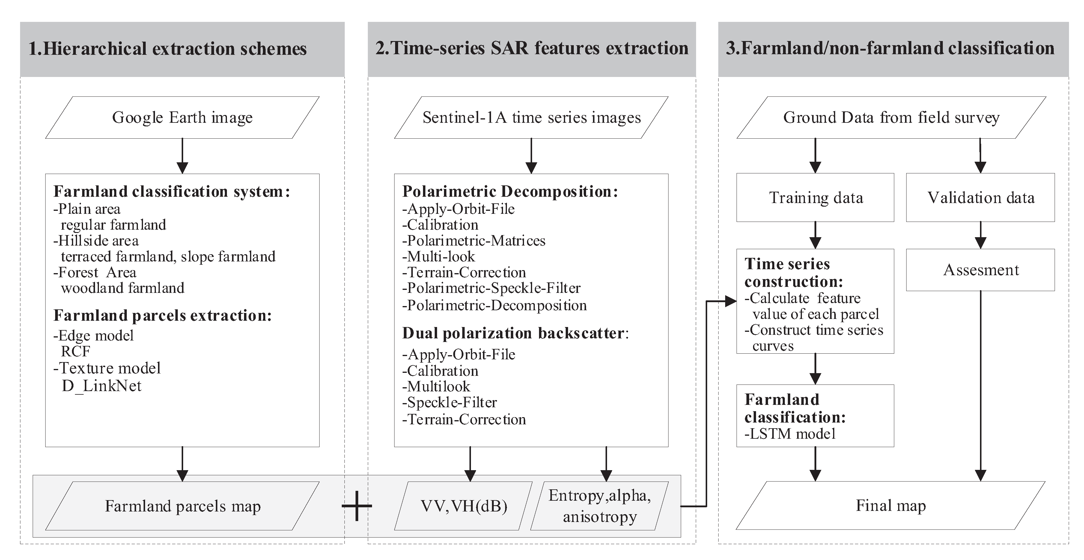
Reference data is necessary to generate a land cover map, especially a farmland distribution map. For classifier calibration and output validation, a field survey was conducted in May 2019 to collect sampling points, which present a detailed description of the land cover and locations, using GPS-enabled tablets. We subsequently delineated the reference parcels for which the sampling points were collected. The boundaries of these parcels were delineated by manual visual interpretation using the Google satellite imagery mentioned in Section 2.2 as a reference, and the land cover type of each parcel is consistent with its internal sampling points. Additional samples of underrepresented classes are also supplemented by this image. We finally obtained 913 sample parcel objects (Table 2), including farmland (such as rice, rape, soybeans, corn, and vegetables) and non-farmland (such as woodland, grassland, urban areas, and water.).

3. Method

In this study, we propose a method for precise farmland parcel mapping in mountainous areas. The proposed method architecture is elaborated in this section, as shown in Figure 2, which mainly includes three parts:
  • hierarchical extraction schemes using VHR optical images, consisting of a farmland parcel classification system and CNN-based farmland parcel extraction;
  • time-series SAR features extraction from the S1A dataset;
  • farmland/non-farmland classification using time series SAR data, consisting of parcel-level time-series feature construction and LSTM-based classification.

3.1. Hierarchical Extraction Scheme Uusing VHR Optical Images

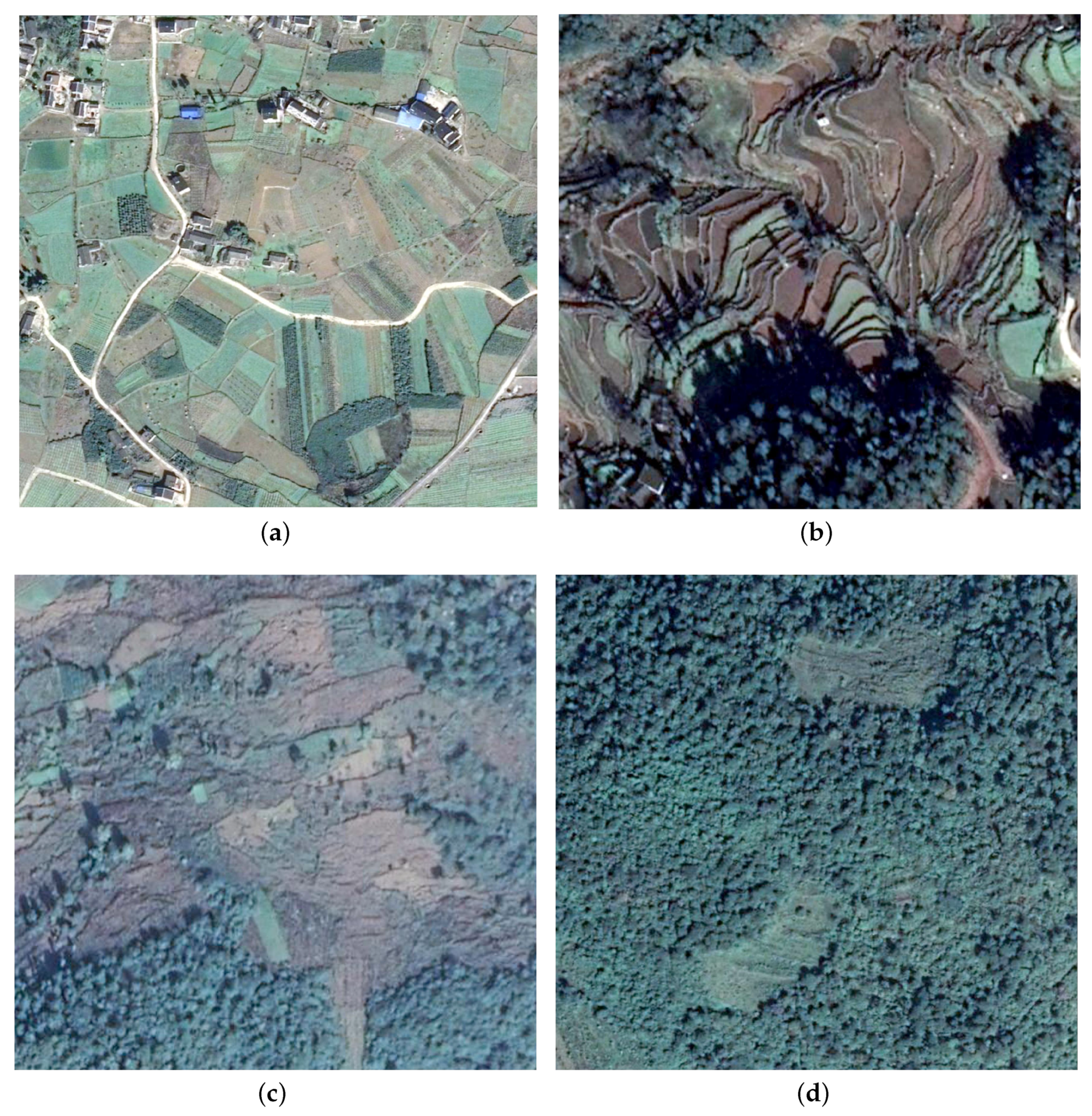
3.1.1. Farmland Classification System Based on Geographical Divisions

Due to the distinguishing topographic conditions in the mountainous areas, the farmland objects present different spatial morphological characteristics, which also leads to the complexity and difficulty of state-of-the-art farmland parcel extraction methods based on deep learning technology. Therefore, a hierarchical farmland classification system was designed for this study, by the visual characteristics of the farmland presented in VHR images. This classification system consists of two levels (Table 3), divides the mountain area into three main geographic sub-regions, and produces four main farmland types distributed in different sub-regions, respectively. Subsequently, we separately conducted the four types of farmland extraction using VHR optical images from Google Earth, which is shown in detail in Section 3.1.2.
In the first level, the entire study area was divided into three geographic sub-regions based on topographical characteristics, namely, plain areas, hillside areas, and forest areas. Due to the relatively consistent geographic conditions, the farmland distributed in each geographical sub-region has similar morphological features on VHR images. The second level aims to divide farmland into four farmland types in different geographical sub-regions, namely regular farmland in plain areas, terraced farmland and slope farmland in hillside areas, and woodland farmland in forest areas, as shown in Figure 3. Among them, woodland farmland represents the farmland with a low degree of reclamation among forests. This carelessly planted farmland, which is scattered among the forest and grass, is very difficult to identify. Therefore, this paper classifies the woodland farmland type as a separate category for extraction.
This hierarchical extraction method allows the complex mountain landscape to be gradually divided into relatively uniform geographic units (farmland parcels), in which finer farmland can be distinguished. The applicability of this farmland extraction method can also be evaluated in different regions. In addition, this method can flexibly use a single-level map (such as slope farmland) or combine maps from multiple levels (such as regular farmland and terraced farmland) to meet other specific needs.

3.1.2. Parcel-Stratified Extraction Based on CNNs

The CNN was used as a classifier because of its representation learning ability, which was used to identify precise target objects from VHR images. However, the performance of existing models is hindered by the complex visual features of the farmland, as well as the substantial VHR image content, which has led to a host of sample production and complex model improvements tasks. Based on the analysis of the visual characteristics of the four farmland types mentioned in Section 3.1.1, a farmland parcel-stratified extraction process was designed, as follows:
  • The deep learning algorithm was selected according to the unique features of target objects. In this study, the Richer Convolutional Features(RCF) model [53] was used for the extraction of parcels with clear boundaries (regular farmland and terraced farmland), and the D_LinkNet model [54] was used to obtain texture-based parcels (slope farmland and woodland farmland). Since we focus on the effect of this hierarchical extraction scheme in complex landscapes, other studies on the improvement of deep learning models for the characteristics of target objects are not discussed in this paper.
  • CNN training requires a relatively large amount of labelled data. The training data for four farmland types were cropped from the VHR satellite images, where the sampled data are not available, and manually delineated through visual-interpretation. The samples of regular farmland and terraced farmland were used to train an edge model, while the samples of slope farmland and woodland farmland were used to train two different texture models, respectively. Through the iterative training method, four farmland types parcel extraction models were respectively generated based on these samples.
  • Due to the higher similarity between regular farmland and terraced farmland, these farmlands were first extracted together. We then used these results as a mask to extract slope farmland in the remaining area. All the obtained parcels were subsequently used together as a mask, and the woodland farmland was finally obtained to ensure that as much farmland as possible was obtained. Finally, through sample addition and iterative training methods, the missing and wrong areas were supplemented and corrected to improve the final map.
To facilitate complete farmland parcel delineations over the study area, all farmland-like parcels were considered in this parcel map, which will be optimized in subsequent farmland/non-farmland classification method.

3.2. Time-Series SAR Feature Extraction

In this study, the S1A dataset was used to generate time-series SAR features. The role of linear polarization backscatter intensity and polarimetric variables were investigated for their effects, and five variables were obtained from each SAR images, consisting of two linear polarizations parameters (VV/VH) and three decomposition parameters (entropy, anisotropy, and alpha angle). The linear polarization intensity value indicates the change in the total energy reflected by the ground. Polarization decomposition obtains the polarization parameters that can characterize the structural features and scattering mechanism of ground objects by deconstructing the polarized SAR signal. The H-A- α decomposition method provided by the Snap platform, derived from the Cloude–Pottier decomposition method [55], was used to process each S1A image and generate three parameters: entropy (H), anisotropy (A), and alpha angle ( α ). Entropy represents the randomness of scattering, with a range from 0 to 1. Anisotropy reveals the relative importance of the secondary scattering mechanism, and this value is a measure of the intensity of scattering, ranging from 0 to 1. The angle alpha indicates the main scattering mechanism, with a range of 0 to 90 , such as surface scattering ( α lower than 40 ), volume or dipole scattering ( α about 45 ), and double rebound scattering ( α more than 50 ) [56,57]. We firstly obtained the backscatter intensity value (dB) for both polarizations (VV, VH), mainly including five steps: Apply-Orbit-File, Calibration, Multilooking, Speckle-Filter, and Terrain-Correction. In order to further analyze the impact of the variables related to the scattering mechanism, we subsequently calculated the polarization decomposition parameters, which mainly include the following seven steps: Apply-Orbit-File, Calibration, Polarimetric-Matrices, Multilooking, Terrain-Correction, Polarimetric-Speckle-Filter, and Polarimetric-Decomposition. In this process, high-precision orbit data and 30 m SRTM-1sec DEM data provide precise geographic location information so that the final result has a high geometric accuracy and can be matched with the Google image mentioned in Figure 1 without manual correction. All this preprocessing of the S1A SAR data was completed in ESA snap software.

3.3. Farmland/Non-Farmland Classification Using Time Series SAR Data

With the obtained results, which include farmland-like parcels, in Section 3.1, the next step in this methodology was to construct temporal features to distinguish farmland parcels from other types. These features (VV, VH, alpha angle, anisotropy, and entropy) were generated from the processed S1A dataset. Hence, for the automatic mapping of precise farmland parcels, we need a reliable method to identify the types of farmland/non-farmland parcels by investigating the farmland throughout the year.

3.3.1. Time Series Features Construction

Recent studies have shown that the linear SAR backscatter value of farmland has an obvious change pattern, which is related to the type of plant [58]. In addition, due to the ability to characterize the structural characteristics and scattering mechanism of ground targets, there are also obvious change patterns in polarization decomposition parameters, which are affected by the plant structure and growth [59]. Therefore, this study investigates the farmland classification using the linear backscattering intensity and polarization decomposition parameters. For each SAR image, the mean value of pixels inside a parcel is considered as the feature value of that parcel. We finally obtained five time series curves for each parcel from the S1A dataset, consisting of two linear polarizations (VV, VH) and three H-A- α decomposition parameters (H, A, and α ). This method of calculating the mean value of pixels also helps to remove the speckle effect of the SAR data. The reference data (Section 2.3) is also processed in this way to generate training and validation samples.

3.3.2. Classification Model Based on LSTM

RNNs can only have short-term memory due to the problem of gradient disappearance or explosion. As one of the best performing RNN units, long-term memory (LSTM) can learn long-term dependence and express the characteristics of sequence changes, which is widely used in time series analysis [60]. Hence, we choose the LSTM unit as the recursive unit in our research. Formulas (1)–(6) formally describe the LSTM neuron [50,52].
The LSTM unit consists of two cell states—the memory c t and the hidden state h t —and three different gates—the input ( i t ), the forget ( f t ), and the output ( o t ), which are used to control the flow of information. These three gates combine the current input x t with the hidden state h t 1 of the previous step and filter the information in this process to solve the problem of gradient disappearance/explosion. These gates are implemented by a sigmoid, which gives values between 0 and 1. A new content memory cell y t is also been used to adjust the current input, which is implemented by a hyperbolic tangent function. As shown in Equations (1) and (2), the input i t specifies how much information needs to be retained in the memory cell, and the forget gate f t decides the extent to which the existing stored content is forgotten, as shown in Equation (3). Equation (4) indicates that the memory state c t can be updated by the input ( i t ), the forget ( f t ), and the last memory state c t 1 . Finally, the output gate o t determines how much current memory content can be output to the next step and impacts the new hidden state ( h t ), which is exported as shown in Equations (5) and (6). The memory c t and the hidden state h t ) are both used as part of the input at the next step.
i t = σ W i x x t + W i h h t 1 + b i
y t = tanh W y x x t + W y h h t 1 + b y
f t = σ W f x x t + W f h h t 1 + b f
c t = i t y t + f t c t 1
o t = σ W o x x t + W o h h t 1 + b o
h t = o t tanh c t
where W denote weight matrices. b o is the deviation coefficient of the model.
In this article, we determined the optimal parameter values in LSTM by an experimental method, the detailed experiment as shown in Section 4.5. Eventually, a two-layer LSTM network with 18 hidden neurons was used for time-series sequence classification, as shown in Figure 4.

3.4. Accuracy Assessment

We used the overall accuracy (OA), producer’s accuracy (PA), user’s accuracy (UA), and F1-score to evaluate and compare the accuracies of the farmland parcel maps, which were obtained by the hierarchical extraction scheme and the farmland/non-farmland classification method (Stage 2 and 3 in Table 4):
OA = T P + T N T P + T N + F P + F N
PA = T P T P + F P
UA = T P T P + F N
F 1 s c o r e = 2 × PA × UA PA + UA
where TP, TN, FP, and FN represent the true positive, true negative, false positive, and false negative pixels in the parcel extraction results, and are calculated by comparing the extracted data with the reference data at each of the sampled pixels.
In addition, we further evaluated the performance of LSTM-based classifier (Table 5, Figures 8 and 9), where TP, TN, FP, and FN represent the true positive, true negative, false positive, and false negative parcels in the classification results, and are computed by comparing the classified parcels with the sampled parcels. Since the sample dataset is relatively small, we performed a 10-fold cross-validation on the sample dataset for each classification. The 913 sampled parcels were divided into ten equal subsets, and one of them was used as the validation dataset and the others were used as the training dataset in each fold. Moreover, each subset was selected using spatial partitions, so as to make sure that training and validation datasets are taken from different areas. It is also noted that we choose each subset according to the approximate proportion of the number of categories in the field sampling data. All classification accuracies were averaged across the ten validations.

4. Results

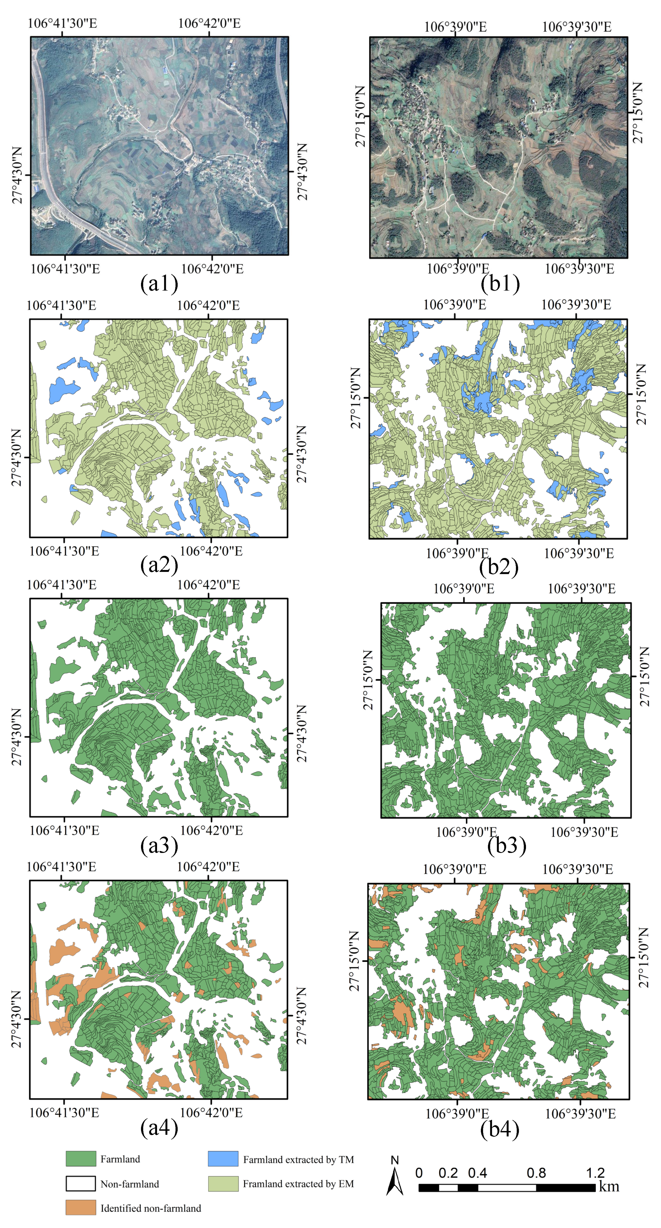
4.1. Overall Farmland Parcel Extraction Results

Figure 5 shows the final farmland parcel distribution map of the study area. This paper final obtained 156,965 farmland parcels in total, with an average area of 0.0935 ha. The area of the parcel is mainly between 0.01 ha and 0.5 ha, accounting for 90%. This also shows the characteristics of small and broken farmland parcels in mountainous areas.
The method proposed in this paper mainly includes two steps: a hierarchical extraction scheme using VHR optical imagery and a farmland classification using a time series SAR dataset. Therefore, we divided the extraction process into three stages, Stages 1, 2, and 3, to evaluate the enhancement of these methods on the mapping results, as shown in Figure 6. Stage 1 obtains farmland parcels by only an edge model (EM), which is shown in Figure 6(a2,b2) (apple dust parcels). Stage 2 refers to the use of a texture model (TM) on the basis of Stage 1 to obtain slope farmland and woodland farmland (blue parcels in Figure 6(a2,b2)). These two stages together constitute the hierarchical extraction scheme, and the result is displayed in Figure 6(a3,b3). In the final stage, the farmland classification method based on LSTM is used to eliminate non-farmland to further optimize the obtained results before. The accuracies of these stages are shown in Table 4.

4.2. Hierarchical Extraction Results

In this part, we focus on the delineation of farmland parcels and ensure that all farmland parcels in the study area are included in the obtained results. Hence, the producer’s accuracy (PA) of farmland extraction is the indicator we pay attention to in this step, because it represents the error of omission. As shown in Table 4, the overall accuracy between the two stages does not differ significantly (87.47% and 87.56%), which is due to a host of non-farmland types in the results of Stage 2. However, the hierarchical extraction scheme (Stage 2) resulted in an extremely higher PA of farmland extraction, reaching 96.38%, while the PA of Stage 1 was only 88.99%, which is conducive to the farmland type identification in the next stage.

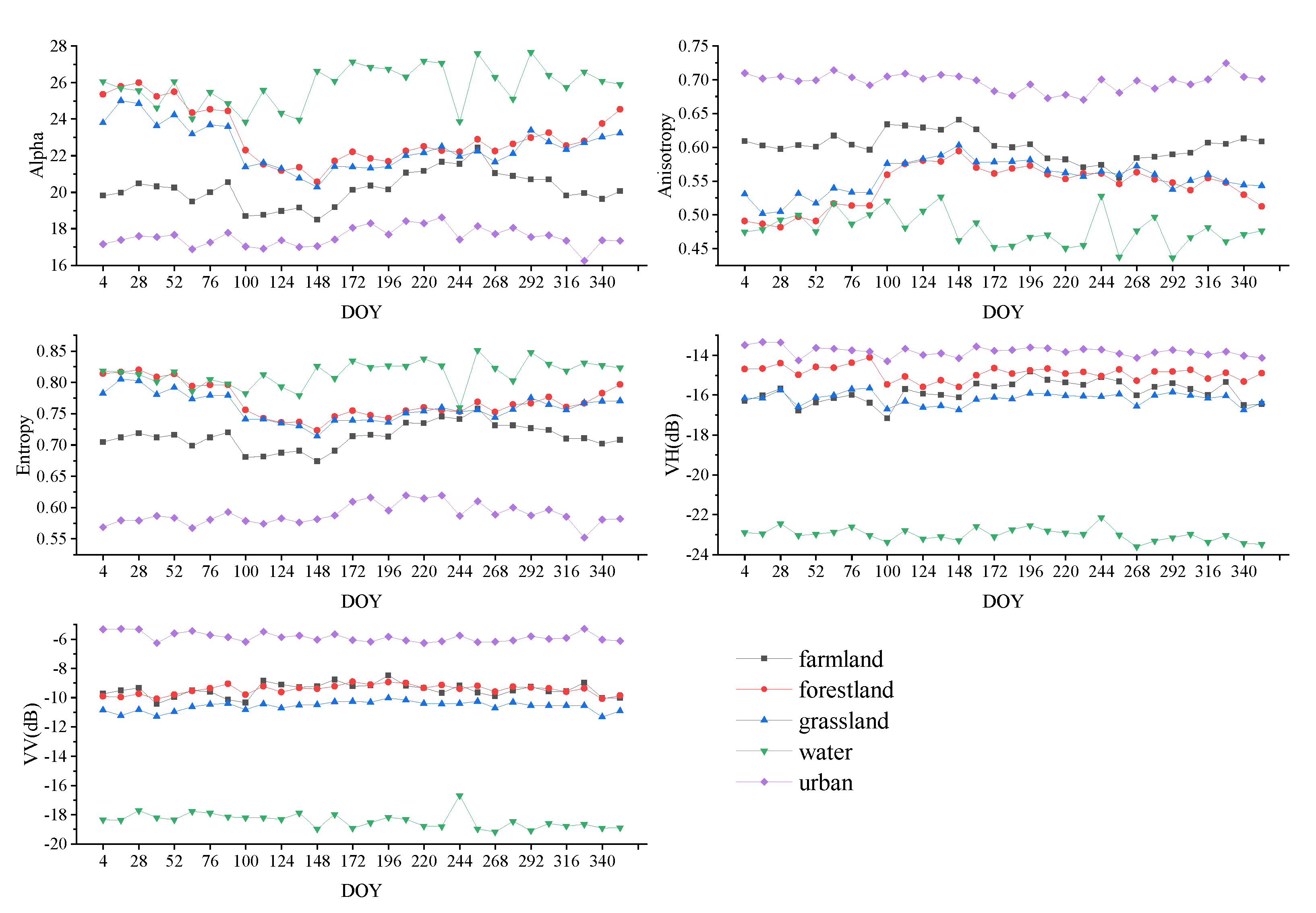
4.3. Time Series Feature Construction Results

We established the annual time series curves of farmland, forestland, grassland, water, and urban areas from the S1A image datasets related to the ground truth pixels in the field sampled parcels, including VV (dB), VH (dB), entropy, anisotropy, and alpha angle ( α ). Figure 7 shows the constructed temporal profiles of the farmland class and four non-farmland classes per metric.
By comparing the temporal behavior of farmland and other types, we observe that farmland parcels have significantly different temporal behaviors in terms of entropy, alpha, and anisotropy. The time series curves from DOY 4 to DOY 160 and from DOY 292 to DOY 352 are especially distinguishable. However, it is difficult to distinguish farmland from woodland and grassland in the temporal curves during the middle of the year (DOY 160 to DOY 280). For VV and VH, the time behavior of farmland is very easy to distinguish from that of water and buildings. Yet the VH time series curves of farmland and grassland have similar time curves between DOY 4 and DOY 100. For the VV signal, forestland and farmland have similar time series curves throughout the year.

4.4. Farmland/Non-Farmland Classification Results

As shown in a4 and b4 of Figure 6, in Stage 3, we implemented a time series classification method based on LSTM to distinguish farmland/non-farmland types, so as to obtain an accurate farmland distribution map. Five radar parameters from the 30 S1A image datasets were used to assess the capability of time series SAR data for identifying farmland parcels. We obtained the classification accuracy about VV, VH, Entropy, anisotropy, and alpha angle time series, including UA, PA, OA, and F1-scores. Table 5 shows that an overall accuracy of 80.83% was obtained when performing 10-fold cross-validation with five variables. Farmland parcels obtained an especially high accuracy, with a producer’s accuracy of 89.02%, a user’s accuracy of 78.80%, and an F1 score of 0.8360. Therefore, in stage 3, non-farmland parcels are identified and removed using this LSTM-based classification method, resulting in an very high overall accuracy of 96.05% in the final farmland parcels map (Table 4).
To investigate the impact of variables on classification accuracy, we subsequently compared the accuracy of classification using different variables. For a single variable, alpha has the highest accuracy among all variables, with an overall accuracy of 0.7689. The linear polarization intensity and polarization decomposition parameters represent the different characteristics of ground objects. When only using polarization decomposition variables, the overall accuracy is 0.7776, and the F1-score of the farmlands is 0.8146. In comparison, the overall accuracy and F1-score of only using linear polarization are increased by 1.42% and 1.14%, respectively, reaching 0.7918 and 0.8260. This result demonstrates the contribution of linear polarization variables to farmland extraction.

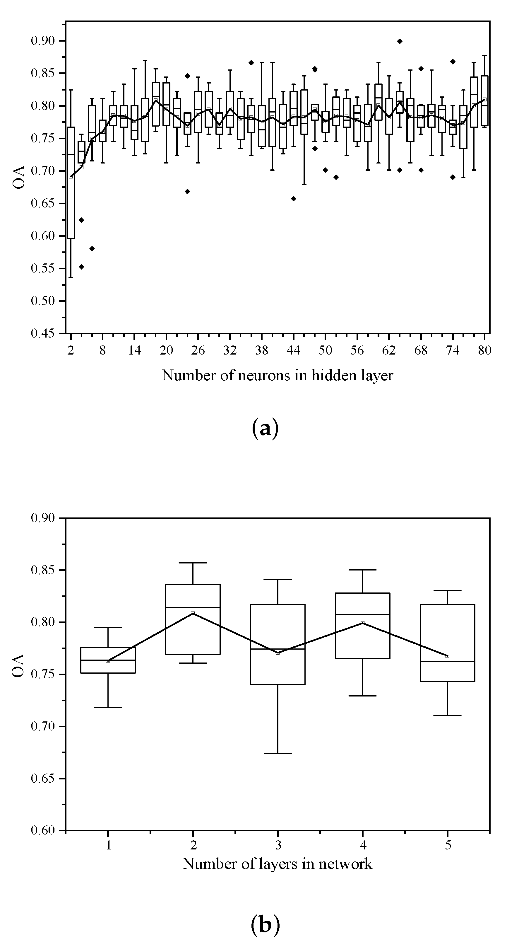
4.5. Parameter Setting in the LSTM-Based Classification Model

The number of neurons in the hidden layer and network layers are important parameters of LSTM, which have a great impact on the classification performance. Figure 8 shows how the overall accuracy of LSTM classification varies with the number of neurons in the hidden layer and the number of network layers. The number of neurons range from 2 to 80 with a step of 2, and the number of network layers range from 1 to 5 with a step of 1. Figure 8 also shows the standard deviation, which represents the stability of the model classification and is represented in the box plot in this figure. For the current limited data, a network that is too complex or too simple can easily lead to overfitting or underfitting. Hence, after extensive training and comprehensive consideration of the accuracy and stability of classification, we set up the optimal network parameter configuration, with 18 neurons and 2 network layers.
In order to get the best time series combination, we evaluated the classification accuracy of different time series, as shown in Figure 9. The growth of the OA indicates that the added period data is conducive to the farmland classification. The overall classification accuracy increases as the number of time-series images increases, reaching the highest accuracy at DOY 172. In the middle of the year (between DOY 172 and DOY 268), the OA enters a stable state before DOY 268). This change is consistent with the analysis in Section 4.3. The period between DOY 172 and DOY 268) represents the season of plant growth, during which the characteristics of crops change more obviously. However, the rainy weather in the area and the careless planting lead to difficulty in distinguishing the wasteland from the farmland, so the time series features of this period fails to improve the classification accuracy. The harvest of the main crops caused the curve to drop rapidly at DOY 292 and then gradually increased. Therefore, the relatively dry period is more conducive to identifying the types of farmland parcels, which is also the main planting season of rape, that is, the time series after DOY 292 in the previous year and before DOY 172 in the following year.

5. Discussion

In this paper, we propose a novel method to map precise farmland distribution in mountainous areas. The method has the following characteristics:
  • The advantages of VHR optical data and time series SAR data are combined. VHR Google satellite optical imagery is used for obtaining basic parcels for farmland mapping, and the S1A SAR dataset provides time-series features for identifying the farmland parcels.
  • The hierarchical extraction scheme based on a divided and stratified strategy greatly reduces the difficulty of obtaining farmland parcels in complex scenes. By dividing the ground objects layer by layer, these objects are extracted at a relatively simple level, so the design and training of the model can be conducted at a lower cost. It is worth noting that the distinguishability between each extracted object class affects the extraction accuracy. Low distinguishability will cause the same object to be extracted by different models, which affects the accuracy of the results. This is also the reason why the overall accuracy of Stage 2 shown in Table 4 has not increased compared to Stage 1. However, in this step, we focus on obtaining the parcel objects containing all the farmland and identifying them through subsequent time series classification. Therefore, this problem does not affect the results of the proposed method.
  • The CNN-based parcel extraction method is different from the previous method of object segmentation, and the obtained parcel objects more closely matches the shape of the ground objects.
  • Recent studies [56,61] have shown great potential of polarization decomposition variables for crop classification. However, in this study, linear polarization variables produced a higher accuracy. This is because, in complex agricultural landscapes, such as mountainous areas, consisting of various types of crops, polarization decomposition variables that reflect the different scattering mechanisms of land covers are more suitable than linear polarization variables for the identification of high biomass crops, but do not have an advantage in the identification of agricultural landscapes with various crops.
  • Compared with the pixel-level method, this paper assigned the mean value of all pixels in the parcel as the feature value of this parcel, thereby reducing the influence of SAR speckle noise.
Through the experiment in the southwest mountainous areas of China, the proposed method in this paper shows excellent performance for the farmland extraction in complex scenes. However, there are still some problems in this article, which can be improved in the future.
  • In this experiment, farmland types are classified by only visual features, leading to the acquisition of other types of parcels. We should consider using other geographic element features (such as elevation, slope, and water content) to improve discrimination for more detailed classifications. As type discrimination increases, more accurate and complete extraction results can be obtained.
  • There are some extremely fragmented and small farmland parcels in mountainous areas that are hard to extract, and the temporal behavior of these parcels is also difficult to construct from the S1A dataset. Therefore, the parcel extraction model needs to be further optimized to improve the acquisition ability of small boundaries, and higher spatial resolution SAR data should be obtained to generate the time profiles of these parcels.
  • In smallholder agricultural areas, the crop temporal behaviors vary from field to field due to the different types of crops and planting time, which leads to the offset of the time series curve of farmland that the model fits, thus reducing the classification accuracy.
  • We also need to obtain more features of farmland parcels from multi-source data, so as to identify farmland in a higher dimensional space and achieve greater accuracy.

6. Conclusions

The complex landscape conditions and the absence of optical data in mountainous areas severely hinder the mapping of precision farmland parcels. In this study, we proposed a new automatic mapping approach for delineating farmland parcels in mountainous areas. The main purpose of this paper is to establish a multi-step extraction framework that integrates the superiority of VHR optical images, time series SAR data, and deep learning technology for obtaining precise parcel objects in complex scenes. The experiment conducted in Southwest China using sub-meter Google satellite imagery and 30 Sentinel-1A images shows the excellent performance of this method.
Through the hierarchical extraction scheme, CNNs can successfully delineate the precise boundaries of ground parcels from VHR images in mountainous areas. By the verification of visual inspection, the delineations of the obtained parcels are close to the level of human visual interpretation. The good PA of farmland parcels (>95%) also indicates the remarkable ability of this method for obtaining precise ground objects in complex scenes. These parcels, as the processing units of the time series classification, provide an important basis for mapping farmland distribution. In addition, with the LSTM-based time series classification method, we have noticed the beneficial value of SAR backscattering variables for farmland identification in cloudy and rainy areas (OA > 80%). Linear polarization variables, compared to the polarization decomposition variables, are more suitable for the farmland classification under the conditions of complex planting structures in mountainous areas. Moreover, this method converts the research object from pixels to parcels, which greatly reduces the influence of SAR data speckle noise. These study results show that the proposed method can also be used for the identification of other land types under complex landscape conditions and can be extended to any other region. However, there are still some aspects that need to be further explored.
In future research, we will explore how more discriminating classification rules can be introduced, and more targeted parcel extraction algorithms, by combining other edge and shape detection methods, will be designed. In addition, other indicators from different data sources, such as multi-band SAR data, may be useful in improving farmland identification accuracy.

Author Contributions

W.L. proposed the research methodology, prepared the data, performed and analyzed the experiments, and wrote the manuscript. J.W. helped conduct the experiments and analysis. J.L. outlined the research topic and acquired the funding. Z.W., Z.S. and Y.Z. made great contributions to manuscript reviewing and editing. J.C. and Y.S. assisted with data preparation and manuscript writing. N.X. and Y.Y. helped to conduct and validate the experiment. All authors have read and agreed to the published version of the manuscript.

Funding

This research was funded by the National Key R&D Program of China (grant number 2018YFD1100301), the National Natural Science Foundation of China (grant number 41631179, 41971375), and the NSFC-Guangdong Joint Foundation Key Project (grant number U1901219).

Conflicts of Interest

The authors declare that there is no conflict of interest.

Abbreviations

The following abbreviations are used in this manuscript:
VHRVery High Resolution
SARSynthetic Aperture Radar
CNNsConvolutional Neural Networks
RNNsRecurrent Neural Networks
LSTMLong and Short-Term Memory

References

  1. Ashourloo, D.; Shahrabi, H.S.; Azadbakht, M.; Aghighi, H.; Nematollahi, H.; Alimohammadi, A.; Matkan, A.A. Automatic canola mapping using time series of sentinel 2 images. ISPRS J. Photogramm. Remote Sens. 2019, 156, 63–76. [Google Scholar] [CrossRef]
  2. Skakun, S.; Kussul, N.; Shelestov, A.; Kussul, O. The use of satellite data for agriculture drought risk quantification in Ukraine. Geomat. Nat. Hazards Risk 2016, 7, 901–917. [Google Scholar] [CrossRef]
  3. Sulik, J.J.; Long, D.S. Spectral considerations for modeling yield of canola. Remote Sens. Environ. 2016, 184, 161–174. [Google Scholar] [CrossRef] [Green Version]
  4. Persello, C.; Tolpekin, V.A.; Bergado, J.R.; de By, R.A. Delineation of agricultural fields in smallholder farms from satellite images using fully convolutional networks and combinatorial grouping. Remote Sens. Environ. 2019, 231, 111253. [Google Scholar] [CrossRef]
  5. Burke, M.; Lobell, D.B. Satellite-based assessment of yield variation and its determinants in smallholder African systems. Proc. Natl. Acad. Sci. USA 2017, 114, 2189–2194. [Google Scholar] [CrossRef] [Green Version]
  6. Kontgis, C.; Schneider, A.; Ozdogan, M. Mapping rice paddy extent and intensification in the Vietnamese Mekong River Delta with dense time stacks of Landsat data. Remote Sens. Environ. 2015, 169, 255–269. [Google Scholar] [CrossRef]
  7. Massey, R.; Sankey, T.T.; Congalton, R.G.; Yadav, K.; Thenkabail, P.S.; Ozdogan, M.; Sánchez Meador, A.J. MODIS phenology-derived, multi-year distribution of conterminous U.S. crop types. Remote Sens. Environ. 2017, 198, 490–503. [Google Scholar] [CrossRef]
  8. Zhong, L.; Hu, L.; Le, Y.; Gong, P.; Biging, G.S. Automated mapping of soybean and corn using phenology. ISPRS J. Photogramm. Remote Sens. 2016, 119, 151–164. [Google Scholar] [CrossRef] [Green Version]
  9. Bouvet, A.; Le Toan, T. Use of ENVISAT/ASAR wide-swath data for timely rice fields mapping in the Mekong River Delta. Remote Sens. Environ. 2011, 115, 1090–1101. [Google Scholar] [CrossRef] [Green Version]
  10. Brian, D.W.; Stephen, L.E. Large-area crop mapping using time-series MODIS 250 m NDVI data: An assessment for the U.S. Central Great Plains. Remote Sens. Environ. 2008, 112, 1096–1116. [Google Scholar] [CrossRef]
  11. Sun, C.; Bian, Y.; Zhou, T.; Pan, J. Using of Multi-Source and Multi-Temporal Remote Sensing Data Improves Crop-Type Mapping in the Subtropical Agriculture Region. Sensors 2019, 19, 2401. [Google Scholar] [CrossRef] [PubMed] [Green Version]
  12. Blaschke, T.; Hay, G.J.; Kelly, M.; Lang, S.; Hofmann, P.; Addink, E.; Queiroz Feitosa, R.; van der Meer, F.; van der Werff, H.; van Coillie, F.; et al. Geographic Object-Based Image Analysis—Towards a new paradigm. ISPRS J. Photogramm. Remote Sens. 2014, 87, 180–191. [Google Scholar] [CrossRef] [PubMed] [Green Version]
  13. Castillejo-González, I.L.; López-Granados, F.; García-Ferrer, A.; Manuel Peña-Barragán, J.; Jurado-Expósito, M.; Sánchez de la Orden, M.; González-Audicana, M. Object- and pixel-based analysis for mapping crops and their agro-environmental associated measures using QuickBird imagery. Comput. Electron. Agric. 2009, 68, 207–215. [Google Scholar] [CrossRef]
  14. McCarty, J.; Neigh, C.; Carroll, M.; Wooten, M. Extracting smallholder cropped area in Tigray, Ethiopia with wall-to-wall sub-meter WorldView and moderate resolution Landsat 8 imagery. Remote Sens. Environ. 2017, 202, 142–151. [Google Scholar] [CrossRef]
  15. Belgiu, M.; Csillik, O. Sentinel-2 cropland mapping using pixel-based and object-based time-weighted dynamic time warping analysis. Remote Sens. Environ. 2017, 204, 509–523. [Google Scholar] [CrossRef]
  16. Jin, Z.; Azzari, G.; You, C.; Di Tommaso, S.; Aston, S.; Burke, M.; Lobell, D.B. Smallholder maize area and yield mapping at national scales with Google Earth Engine. Remote Sens. Environ. 2019, 228, 115–128. [Google Scholar] [CrossRef]
  17. Yang, J.; Price, B.; Cohen, S.; Lee, H.; Yang, M.H. Object Contour Detection with a Fully Convolutional Encoder-Decoder Network. In Proceedings of the IEEE Conference on Computer Vision and Pattern Recognition (CVPR), Las Vegas, NV, USA, 27–30 June 2016; pp. 193–202. [Google Scholar] [CrossRef] [Green Version]
  18. Xie, S.; Tu, Z. Holistically-Nested Edge Detection. Int. J. Comput. Vis. 2017, 125, 3–18. [Google Scholar] [CrossRef]
  19. Richter, G.M.; Agostini, F.; Barker, A.; Costomiris, D.; Qi, A. Assessing on-farm productivity of Miscanthus crops by combining soil mapping, yield modelling and remote sensing. Biomass Bioenergy 2016, 85, 252–261. [Google Scholar] [CrossRef] [Green Version]
  20. Rosentreter, J.; Hagensieker, R.; Waske, B. Towards large-scale mapping of local climate zones using multitemporal Sentinel 2 data and convolutional neural networks. Remote Sens. Environ. 2020, 237, 111472. [Google Scholar] [CrossRef]
  21. Paoletti, M.E.; Haut, J.M.; Plaza, J.; Plaza, A. A new deep convolutional neural network for fast hyperspectral image classification. ISPRS J. Photogramm. Remote Sens. 2018, 145, 120–147. [Google Scholar] [CrossRef]
  22. Zhang, C.; Sargent, I.; Pan, X.; Li, H.; Gardiner, A.; Hare, J.; Atkinson, P.M. An object-based convolutional neural network (OCNN) for urban land use classification. Remote Sens. Environ. 2018, 216, 57–70. [Google Scholar] [CrossRef] [Green Version]
  23. Maggiori, E.; Tarabalka, Y.; Charpiat, G.; Alliez, P. Convolutional Neural Networks for Large-Scale Remote-Sensing Image Classification. IEEE Trans. Geosci. Remote Sens. 2017, 55, 645–657. [Google Scholar] [CrossRef] [Green Version]
  24. Chen, Y.; Jiang, H.; Li, C.; Jia, X.; Ghamisi, P. Deep Feature Extraction and Classification of Hyperspectral Images Based on Convolutional Neural Networks. IEEE Trans. Geosci. Remote Sens. 2016, 54, 6232–6251. [Google Scholar] [CrossRef] [Green Version]
  25. Castelluccio, M.; Poggi, G.; Sansone, C.; Verdoliva, L. Land Use Classification in Remote Sensing Images by Convolutional Neural Networks. arXiv 2015, arXiv:1508.00092v1. Available online: https://arxiv.org/pdf/1508.00092.pdf (accessed on 1 August 2015).
  26. Hu, W.; Huang, Y.; Wei, L.; Zhang, F.; Li, H. Deep Convolutional Neural Networks for Hyperspectral Image Classification. J. Sens. 2015, 2015, 12. [Google Scholar] [CrossRef] [Green Version]
  27. Gong, Y.; Xiao, Z.; Tan, X.; Sui, H.; Xu, C.; Duan, H.; Li, D. Context-Aware Convolutional Neural Network for Object Detection in VHR Remote Sensing Imagery. IEEE Trans. Geosci. Remote Sens. 2020, 58, 34–44. [Google Scholar] [CrossRef]
  28. Cheng, G.; Zhou, P.; Han, J. Learning Rotation-Invariant Convolutional Neural Networks for Object Detection in VHR Optical Remote Sensing Images. IEEE Trans. Geosci. Remote Sens. 2016, 54, 7405–7415. [Google Scholar] [CrossRef]
  29. Ding, P.; Zhang, Y.; Deng, W.J.; Jia, P.; Kuijper, A. A light and faster regional convolutional neural network for object detection in optical remote sensing images. ISPRS J. Photogramm. Remote Sens. 2018, 141, 208–218. [Google Scholar] [CrossRef]
  30. Nogueira, K.; Penatti, O.A.; dos Santos, J.A. Towards better exploiting convolutional neural networks for remote sensing scene classification. Pattern Recognit. 2017, 61, 539–556. [Google Scholar] [CrossRef] [Green Version]
  31. Hu, F.; Xia, G.S.; Hu, J.; Zhang, L. Transferring Deep Convolutional Neural Networks for the Scene Classification of High-Resolution Remote Sensing Imagery. Remote Sens. 2015, 7, 14680–14707. [Google Scholar] [CrossRef] [Green Version]
  32. Zhang, L.; Zhang, L.; Du, B. Deep Learning for Remote Sensing Data: A Technical Tutorial on the State of the Art. IEEE Geosci. Remote Sens. Mag. 2016, 4, 22–40. [Google Scholar] [CrossRef]
  33. Huang, B.; Zhao, B.; Song, Y. Urban land-use mapping using a deep convolutional neural network with high spatial resolution multispectral remote sensing imagery. Remote Sens. Environ. 2018, 214, 73–86. [Google Scholar] [CrossRef]
  34. Wu, B.; Li, Q. Crop planting and type proportion method for crop acreage estimation of complex agricultural landscapes. Int. J. Appl. Earth Obs. Geoinf. 2012, 16, 101–112. [Google Scholar] [CrossRef]
  35. Fenske, K.; Feilhauer, H.; Förster, M.; Stellmes, M.; Waske, B. Hierarchical classification with subsequent aggregation of heathland habitats using an intra-annual RapidEye time-series. Int. J. Appl. Earth Obs. Geoinf. 2020, 87, 102036. [Google Scholar] [CrossRef]
  36. Haest, B.; Vanden Borre, J.; Spanhove, T.; Thoonen, G.; Delalieux, S.; Kooistra, L.; Mücher, C.; Paelinckx, D.; Scheunders, P.; Kempeneers, P. Habitat Mapping and Quality Assessment of NATURA 2000 Heathland Using Airborne Imaging Spectroscopy. Remote Sens. 2017, 9, 266. [Google Scholar] [CrossRef] [Green Version]
  37. Potgieter, A.B.; Apan, A.; Hammer, G.; Dunn, P. Early-season crop area estimates for winter crops in NE Australia using MODIS satellite imagery. ISPRS J. Photogramm. Remote Sens. 2010, 65, 380–387. [Google Scholar] [CrossRef]
  38. Steele-Dunne, S.C.; McNairn, H.; Monsivais-Huertero, A.; Judge, J.; Liu, P.; Papathanassiou, K. Radar Remote Sensing of Agricultural Canopies: A Review. IEEE J. Sel. Top. Appl. Earth Obs. Remote Sens. 2017, 10, 2249–2273. [Google Scholar] [CrossRef] [Green Version]
  39. Song, P.; Mansaray, L.R.; Huang, J.; Huang, W. Mapping paddy rice agriculture over China using AMSR-E time series data. Isprs J. Photogramm. Remote Sens. 2018, 144, 469–482. [Google Scholar] [CrossRef]
  40. Veloso, A.; Mermoz, S.; Bouvet, A.; Le Toan, T.; Planells, M.; Dejoux, J.F.; Ceschia, E. Understanding the temporal behavior of crops using Sentinel-1 and Sentinel-2-like data for agricultural applications. Remote Sens. Environ. 2017, 199, 415–426. [Google Scholar] [CrossRef]
  41. Jiao, X.; Kovacs, J.M.; Shang, J.; Mcnairn, H.; Walters, D.; Ma, B.; Geng, X. Object-oriented crop mapping and monitoring using multi-temporal polarimetric RADARSAT-2 data. Isprs J. Photogramm. Remote Sens. 2014, 96, 38–46. [Google Scholar] [CrossRef]
  42. Homayouni, S.; Mcnairn, H.; Hosseini, M.; Jiao, X.; Powers, J. Quad and compact multitemporal C-band PolSAR observations for crop characterization and monitoring. Int. J. Appl. Earth Obs. Geoinf. 2019, 74, 78–87. [Google Scholar] [CrossRef]
  43. Deschamps, B.; Mcnairn, H.; Shang, J.; Jiao, X. Towards operational radar-only crop type classification: Comparison of a traditional decision tree with a random forest classifier. Can. J. Remote Sens. 2012, 38, 60–68. [Google Scholar] [CrossRef]
  44. Sun, Y.; Luo, J.; Wu, T.; Yanan, Z.; Liu, H.; Gao, L.; Dong, W.; Liu, W.; Yang, Y.; Hu, X.; et al. Synchronous Response Analysis of Features for Remote Sensing Crop Classification Based on Optical and SAR Time-Series Data. Sensors 2019, 19, 4227. [Google Scholar] [CrossRef] [PubMed] [Green Version]
  45. Williams, R.; Zipser, D. A Learning Algorithm for Continually Running Fully Recurrent Neural Networks. Neural Comput 1998, 1. [Google Scholar] [CrossRef]
  46. Graves, A.; Mohamed, A.R.; Hinton, G. Speech Recognition with Deep Recurrent Neural Networks. ICASSP IEEE Int. Conf. Acoust. Speech Signal Process.-Proc. 2013, 38. [Google Scholar] [CrossRef] [Green Version]
  47. Mikolov, T.; Karafiát, M.; Burget, L.; Cernocký, J.; Khudanpur, S. Recurrent neural network based language model. In Proceedings of the 11th Annual Conference of the International Speech Communication Association, INTERSPEECH, Makuhari, Chiba, Japan, 26–30 September 2010; pp. 1045–1048. [Google Scholar]
  48. Hinton, G.; Deng, L.; Yu, D.; Dahl, G.; Mohamed, A.R.; Jaitly, N.; Senior, A.; Vanhoucke, V.; Nguyen, P.; Sainath, T.; et al. Deep Neural Networks for Acoustic Modeling in Speech Recognition: The Shared Views of Four Research Groups. IEEE Signal Process. Mag. 2012, 29, 82–97. [Google Scholar] [CrossRef]
  49. Sun, Z.; Di, L.; Fang, H. Using long short-term memory recurrent neural network in land cover classification on Landsat and Cropland data layer time series. Int. J. Remote Sens. 2018, 40, 1–22. [Google Scholar] [CrossRef]
  50. Emile, N.; Dinh, H.T.M.; Nicolas, B.; Dominique, C.; Laure, H. Deep Recurrent Neural Network for Agricultural Classification using multitemporal SAR Sentinel-1 for Camargue, France. Remote Sens. 2018, 10, 1217. [Google Scholar]
  51. Zhou, Y.; Luo, J.; Feng, L.; Yang, Y.; Chen, Y.; Wu, W. Long-short-term-memory-based crop classification using high-resolution optical images and multi-temporal SAR data. GISci. Remote Sens. 2019, 56, 1170–1191. [Google Scholar] [CrossRef]
  52. Dinh, H.; Tong, M.; Ienco, D.; Gaetano, R.; Lalande, N.; Ndikumana, E.; Osman, F.; Maurel, P. Deep Recurrent Neural Networks for mapping winter vegetation quality coverage via multi-temporal SAR Sentinel-1. IEEE Geosci. Remote. Sens. Lett. 2018, 15, 464–468. [Google Scholar] [CrossRef]
  53. Liu, Y.; Cheng, M.M.; Hu, X.; Bian, J.W.; Zhang, L.; Bai, X.; Tang, J. Richer Convolutional Features for Edge Detection. IEEE Trans. Pattern Anal. Mach. Intell. 2019, 41, 1939–1946. [Google Scholar] [CrossRef] [PubMed] [Green Version]
  54. Zhou, L.; Zhang, C.; Wu, M. D-LinkNet: LinkNet with Pretrained Encoder and Dilated Convolution for High Resolution Satellite Imagery Road Extraction. In Proceedings of the 2018 IEEE/CVF Conference on Computer Vision and Pattern Recognition Workshops (CVPRW), Salt Lake City, UT, USA, 18–22 June 2018; pp. 182–186. [Google Scholar] [CrossRef]
  55. Cloude, S.R.; Pottier, E. An entropy based classification scheme for land applications of polarimetric SAR. IEEE Trans. Geosci. Remote Sens. 1997, 35, 68–78. [Google Scholar] [CrossRef]
  56. Li, H.; Zhang, C.; Zhang, S.; Atkinson, P.M. Crop classification from full-year fully-polarimetric L-band UAVSAR time-series using the Random Forest algorithm. Int. J. Appl. Earth Obs. Geoinf. 2020, 87, 102032. [Google Scholar] [CrossRef]
  57. Guo, J.; Wei, P.L.; Liu, J.; Jin, B.; Su, B.F.; Zhou, Z.S. Crop Classification Based on Differential Characteristics of H/α Scattering Parameters for Multitemporal Quad-and Dual-Polarization SAR Images. IEEE Trans. Geosci. Remote Sens. 2018, 56, 6111–6123. [Google Scholar] [CrossRef]
  58. Bazzi, H.; Baghdadi, N.; El Hajj, M.; Zribi, M.; Minh, D.H.T.; Ndikumana, E.; Courault, D.; Belhouchette, H. Mapping Paddy Rice Using Sentinel-1 SAR Time Series in Camargue, France. Remote Sens. 2019, 11, 887. [Google Scholar] [CrossRef] [Green Version]
  59. Whelen, T.; Siqueira, P. Use of time-series L-band UAVSAR data for the classification of agricultural fields in the San Joaquin Valley. Remote Sens. Environ. 2017, 193, 216–224. [Google Scholar] [CrossRef]
  60. Hochreiter, S.; Schmidhuber, J. Long Short-term Memory. Neural Comput. 1997, 9, 1735–1780. [Google Scholar] [CrossRef]
  61. Shuai, G.; Zhang, J.; Basso, B.; Pan, Y.; Zhu, X.; Zhu, S.; Liu, H. Multi-temporal RADARSAT-2 polarimetric SAR for maize mapping supported by segmentations from high-resolution optical image. Int. J. Appl. Earth Obs. Geoinf. 2019, 74, 1–15. [Google Scholar] [CrossRef]
Figure 1. The location of the study area: the green dot represents the location of the sampling point, and the background is a Google satellite image composite of three periods (2 November 2018, 2 February 2019, 7 April 2019).
Remotesensing 12 03733 g001
Figure 2. Workflow of the method proposed in this paper.
Remotesensing 12 03733 g002
Figure 3. The four farmland types presented in Google Earth imagery: (a) regular farmland; (b) terraced farmland; (c) slope farmland; (d) woodland farmland.
Remotesensing 12 03733 g003
Figure 4. The network structure of a classifier based on LSTM.
Remotesensing 12 03733 g004
Figure 5. The distribution map of farmland parcels in the study area using the proposed method. (A,B) are sub-regions of the study area.
Remotesensing 12 03733 g005
Figure 6. Detailed process of the proposed method. (a1,b1) are the sub-regions of the study area; (a2,b2) show farmland parcels extracted using different models (Stage 1); (a3,b3) are the results obtained by the hierarchical scheme using VHR images (Stage 2); (a4,b4) demonstrate the ability to identify non-farmland parcels using SAR temporal features (Stage 3).
Remotesensing 12 03733 g006
Figure 7. Temporal curves of SAR parameters for VV, VH, alpha, anisotropy, and entropy of five classes.
Remotesensing 12 03733 g007
Figure 8. (a) The relationship between classification performance and the number of hidden layer neurons; (b) is the relationship between classification performance and the number of layers in the network.
Remotesensing 12 03733 g008
Figure 9. The relationship between classification performance and time series SAR data. The horizontal axis represents the time series data combination from the fourth day to that time.
Remotesensing 12 03733 g009
Table 1. The Sentinel-1A dataset used in this study.
DataDay of YearDataDay of YearDataDay of Year
4 January 201944 May 20191241 September 2019244
16 January 20191616 May 201913613 September 2019256
28 January 20192828 May 201914825 September 2019268
9 February 2019409 June 20191607 October 2019280
21 February 20195221 June 201917219 October 2019292
5 March 2019643 July 201918431 October 2019304
17 March 20197615 July 201919612 November 2019316
29 March 20198827 July 201920824 November 2019328
10 April 20191008 August 20192206 December 2019340
22 April 201911220 August 201923218 December 2019352
Table 2. Distribution of the reference parcels per class.
Class Number of ParcelsArea (m 2 )Average Area (m 2 )
Farmland 501435,549.88869.36
Non-farmlandUrban98683,677.306976.30
Woodland1481,668,752.8811,275.36
Grassland129595,287.234614.63
Water37248,308.346711.04
Total 9133,631,575.633977.63
Table 3. The farmland classification system.
Level 1 Geographic AreaLevel 2 Farmland TypeFeatures
Plain areaRegular farmlandRegular shape, clear boundaries, uniform internal texture,
and neat spatial distribution.
Hillside areaTerraced farmlandSmall and narrow shape, clear boundaries, uniform internal
texture, and dense spatial distribution.
Slope farmlandVarious shapes, fuzzy boundaries, rough but obvious texture,
and mixed with trees and grass.
Forest areaWoodland farmlandVarious shapes, fuzzy boundaries, grass-like texture, and
scattered between woodland and grassland.
Table 4. Comparision of classification performance between stage 1, stage 2 and stage 3.
StageFarmlandNon-FarmlandOA
PAUAF1PAUAF1
Stage10.88990.88820.88290.86980.87160.86530.8747
Stage20.96380.83070.89300.77150.94820.85150.8756
Stage30.85840.82030.83890.97440.98060.97750.9605
Table 5. Classification performance using different variables.
VariablesFarmlandNon-FarmlandOA
PAUAF1PAUAF1
VV + VH + H + A + α 0.89020.78800.83600.70870.84150.76940.8083
VV+VH0.90020.76310.82600.66020.84470.74110.7918
H+A+ α 0.89020.75080.81460.64080.82760.72230.7776
α 0.88020.74490.80700.63350.81310.71210.7689
H0.88420.73470.80250.61170.81290.69810.7612
VH0.84630.74520.79250.64810.77620.70630.7568
A0.85030.74350.79330.64320.77940.70480.7568
VV0.88220.70380.78300.54850.79300.64850.7317
Publisher’s Note: MDPI stays neutral with regard to jurisdictional claims in published maps and institutional affiliations.

