Coastal Current Intrusions from Satellite Altimetry
by
 and
and
Daniele Casella
1,*, 
Marco Meloni
2,3,
Anne A. Petrenko
4,
Andrea M. Doglioli
4 and
Jerome Bouffard
5 1
Consiglio Nazionale delle Ricerche, Istituto di Scienze dell’Atmosfera e del Clima (CNR-ISAC), 0133 Rome, Italy
2
Serco c/o ESA, European Space Agency ESA-ESRIN, 00044 Frascati, Italy
3
EUMETSAT, Eumetsat Allee 1, 64295 Darmstadt, Germany
4
Aix Marseille Université, Université de Toulon, CNRS, IRD, MIO, 13288 Marseille, France
5
European Space Agency, Directorate of Earth Observation Programmes, 00040 Frascati, Italy
*
Author to whom correspondence should be addressed.
Remote Sens. 2020, 12(22), 3686; https://doi.org/10.3390/rs12223686
Submission received: 21 September 2020
/
Revised: 2 November 2020
/
Accepted: 3 November 2020
/
Published: 10 November 2020
(This article belongs to the Special Issue Observing the Flow of Ocean Currents and Circulation Using Remote Sensing)
Abstract
:The use of satellite-based data in coastal regions for the monitoring of fine-scale ocean dynamics, impacting marine ecosystems, is a difficult challenge. A random forest algorithm to detect slope current intrusions into the Gulf of Lion, Mediterranean Sea, has been developed using both improved coastal altimetry data and 10 year-long numerical simulations. The results have been compared to an independent dataset of in situ measurements from a bottom-moored Acoustic Doppler Current Profiler. The algorithm results are very promising: 93% of slope current intrusions have been correctly identified, and the number of false alarms is moderate. The dependence of the algorithm on several environmental factors is discussed in the paper. From the oceanographic point of view, our results confirm the strong impacts of horizontal winds in the dynamic of the intrusion events in the study area. Our methodology combining numerical modeling, in situ data and new machine-learning tools proves effective in improving the capabilities of ocean remote sensing in coastal areas.
1. Introduction
In the northwestern Mediterranean Sea, the northern portion of the cyclonic circulation is known as the Northern Current (NC) [1]. It flows roughly westward along the continental slope of the Gulf of Lion (GoL). This current is generally warm and oligotrophic. Occasionally, under specific wind conditions, the NC can penetrate the shelf causing an intrusion event (see Figure 1). These events strongly impact the local biogeochemistry [2] and consequntly the primary production because, during the intrusion, the shelf water, rich in nutrients from earlier upwellings, is replaced in 2–3 days by the warmer and oligotrophic NC water. By combining altimetric observations with high-resolution modelling, the relation of intrusion events with the geostrophic currents and horizontal winds has been analyzed in depth, with the objective of developing a machine-learning algorithm for their detection from satellite altimetry.
Previous projects including oceanographic cruises have focused on the detection of NC intrusions [3,4]. These intrusions have also been investigated by Gatti [5] using high-resolution numerical modeling and the results of various oceanographic campaigns. The mechanisms driving the intrusions of the NC into the GoL have also been studied combining in situ observations and high-resolution modeling by Barrier et al. [6], hereafter BPO16. This study demontrates that, on the eastern part of the GoL, current intrusions are forced mainly by strong winds coming predominantly from either the East or the Northwest, each via different physical processes. Easterlies cause a water piling along the coast of the GoL, that through geostrophy, induces an alongshore current intruding the shelf. This current intrusion event is simultaneous with the wind forcing and independent of the sea stratification. Intrusions due to northwesterly winds, on the other hand, occur only in periods of stratified conditions and are associated with upwelling currents near the Var coast (see Figure 1). In particular, a pressure force balances the Coriolis force associated with the deep onshore flow of the upwelling. When the wind calms down, the upwelling and, consequently, the onshore flow and its related Coriolis force weaken. Therefore, the remaining pressure force causes the intrusion of the NC into the GoL shelf about 1 day after the wind relaxation.
The resolution of satellite altimetry, both spatial and temporal, is adequate for monitoring the sea surface height changes in the open ocean (e.g., [7]). However, finer spatial and temporal scales of variability characterize coastal ocean dynamics. In the last decade, coastal altimetry has benefited from major improvements (a recent review can be found in [8]). These improvements include the progress in radar technology (e.g., the use of synthetic aperture radar (SAR) and of the Ka-band), the development of waveform retracking algorithms focused on the coastal areas, and the adoption of improved corrections (e.g., wet troposphere and tidal models), all better adapted to the coastal zone. Compared to previous studies mostly based on sparse in situ observations or on high-resolution models, current coastal altimetry observations are particularly useful for the monitoring of coastal currents, thanks to their high temporal and spatial sampling and to their long-term coherent set of measurements. Some important applications of coastal altimetry techniques in the northern Mediterranean can be found in [9,10,11]. For example, [10] reported an intrusion event into the GoL detected by satellite altimetry. The present work, inspired by [10], improves the detection technique and extends the analysis to a long-term and multi-mission altimetry dataset coupled with in situ data and numerical simulations. The coastal current intrusions are a key process in coastal dynamics, but due to their ephemeral character, they are very hard to observe by oceanographic cruises. Moreover, moorings, if judiciously positioned, can provide time series sufficiently long to observe intrusions, but these data are intrinsically limited in space. Therefore, their detection by satellite, not yet achieved by other works, represents an important development to their observation and study. The algorithm described in this paper has been specifically designed and tuned for the monitoring of coastal current intrusions crossing isobaths, in a specific region of the Mediterranean Sea. However, the methodology used in this work can easily be adapted to other types of oceanic physical processes and other regions. Regions with scarce ground- or coastal-based measurements can particularly benefit from the use of our proposed method to monitor their coastal currents. To adapt this approach to other kind of events or regions, one only need a relatively large dataset of numerical simulations. Regional numerical models are operationally run in a growing number of regions. We want to highlight that the methodology described in this paper is not alternative to numerical modeling, but can be used, together with model forecasts in order to improve the monitoring of harmful current events, such as current intrusions into the GoL.
The intrusion detection algorithm proposed here is based on a random forest algorithm (RFA). This is a popular machine-learning technique, which has already been applied to altimetry data for identifying sea ice thickness [12], sea ice type [13] and oceanic eddies [14]. However, to our knowledge, RFA has never been applied to coastal currents.
2. Materials and Methods
2.1. JULIO Current Meter
Gatti [5] has identified an optimal location for monitoring the current intrusions occurring on the eastern side of the GoL. This site, located on the 100-m isobath at 5.255°E–43.135°N, has been named Judicious Location for Intrusion Observation (JULIO). As such, it has been proposed as a site in the framework of the Mediterranean Ocean Observing System for the Environment (MOOSE) observing system (http://www.moose-network.fr/). JULIO data have been acquired with a bottom-moored Acoustic Doppler Current Profiler (ADCP) (RDI Ocean Sentinel, 300 kHz) during 3 periods: 12 February–23 October 2012; 26 September–31 December 2013; 17 July 2014–10 April 2015. These data sets provide measurements of the horizontal currents with a period of 30 min and with a vertical resolution of 4-m between 15 and 92 m.
BPO16 defined a JULIO index (Jind) for the identification of big current intrusions of the NC on the eastern part of the GoL. In BPO16 Jind is the mean vertical current, projected in a certain direction (49.4°), daily averaged and standardized. We have made some small modifications on Jind compared to the original BPO16 index; but the main calculation remains the same, as now explained. The two small differences (changing the section angle ϑ and not taking into account the boundary layers before the vertical averaging) in the definition of Jind result from a sensitivity study conducted on the SYMPHONIE model simulations that showed that these small changes maximize the correlation with the flux through the 200 m isobath. First, the current has been projected perpendicularly to the JULIO section (at angle ϑ = 57.6° from North in our paper, 49.4° in BPO16; both in a clockwise direction) from the zonal (U) and meridional (V) velocities measured by JULIO:
By convention, Ujul is positive toward the Northwest. Then, Ujul has been vertically averaged, excluding the superficial and deepest currents, i.e., averaging the current profile from −80 m to −1 m (the full profile has been used in BPO16). Then the half-hourly time series have been daily averaged. Finally, the resulting daily time-series have been standardized, i.e., the temporal mean has been removed and the result divided by the standard deviation:
where is the daily average of .
2.2. Altimetry X-TRACK Dataset
An altimetry dataset in the period corresponding to the JULIO measurements and in the region near the GoL has been realized collecting all available measurements from X-TRACK [15]. X-TRACK is a post-processing software, developed by the Center of Topography of the Ocean and Hydrosphere in Toulouse, France, dedicated to improve satellite altimetry in coastal areas. As shown by [15], the most effective improvements in X-TRACK software are the efficient detection of outliers in altimetric corrections and the better reconstruction of the missing or rejected correction values. The authors gave special attention to the determination of the ionospheric, wet tropospheric and sea state bias corrections in coastal areas. Recently [16] X-TRACK became a multi-mission altimetry product applied to all coastal oceans. Moreover, the actual version of X-TRACK includes the Level 2 ALES (Adaptive Leading Edge Subwaveform) retracked product, as well state-of-the-art altimetric corrections. Finally, a new high-resolution (20 Hz) Level 3 product has been made available for research goals. In the present work, all tracks from Jason 2 (J2) and Saral/Altika (SA) in the area 38.5°N–43.7°N and 1°E–8°E, close to the GoL, have been selected. All altimetry data are at 1 Hz resolution and have been used without any further filtering to reduce noise. Table 1 shows some relevant characteristics for each selected track. The selected area is relatively large and some of the selected tracks are relatively far away from JULIO (in some cases more than 250 km). This choice has been taken in order to obtain a sufficient time sampling repetitivity from the two altimeters, as the repeat time periods of J2 and SA are of 10 and 35 days respectively.
2.3. SYMPHONIE Model Simulations
The 3-D primitive equation coastal ocean model SYMPHONIE, described in detail in [17,18], was implemented in a regional configuration [19]. This model is based on the hydrostatic assumption and the Boussinesq approximation. For a detailed description of the SYMPHONIE model see [9] and the references therein.
The SYMPHONIE dataset is built from 10 years of daily simulations (09/01/2001–31/12/2011) over the northern Mediterranean Sea. The simulation domain is a regular grid rotated 31 degrees counterclockwise, with a resolution of about 3 km. The vertical resolution of the model varies with the bathymetry as the vertical levels have been defined in sigma variables.
In this work the SYMPHONIE simulations have been used for several purposes. First, the simulated Sea Surface Heights for each selected altimetry track have been extracted. Then the modeled Sea Level Anomaly (SLA) has been calculated, with a mean value calculated over the 10-year simulations. Second, following [5], the volume flux in the Eastern GoL through the 200 m isobath (F200) has been calculated, by summing the fluxes of interpolated SYMPHONIE currents with 1 km spacing along the curve in Figure 1. Moreover, the currents have been interpolated in the vertical direction every 4 meters. On each interpolating point, the azimuth (az) of the direction normal to the curve has been calculated as well as the component of the oceanic current in that az direction, which corresponds to the current normal to the 200m isobaths with:
Where u and v are the zonal and meridional components of the current. The flux is calculated as the sum of the horizontal currents normal to the vertical portion of sections along the 200 m isobaths. The flux is therefore the sum of all the normal currents multiplied by the area of the summed surfaces (corresponding to ~4000 m2). The normalized flux () is then calculated by subtracting its temporal mean, then dividing by its standard deviation, where both mean value and standard deviation are calculated over the full 10-year SYMPHONIE simulations.
2.4. Horizontal Winds
The horizontal zonal and meridional winds at 10 m over the surface are derived from ECMWF ERA Interim reanalysis dataset (https://www.ecmwf.int/en/forecasts/datasets/reanalysis-datasets/era-interim). These winds have been calculated as the mean daily winds in the position nearest to JULIO in the model grid.
2.5. Random Forests
The random forest is an ensemble learning algorithm (RFA) that combines the ideas of “bootstrap aggregating (bagging)” and “random subspace method” to construct randomized decision trees with controlled variation, introduced by Breiman [20].
In details, in random forest, a recursive partitioning method on a reference data set (learning dataset), builds classification and regression trees (decision trees) for predicting continuous dependent variables (regression) and categorical predictor variables (classification).
Decision trees are represented by a set of questions (if-then logical split conditions on input variables) which splits the learning sample into smaller and smaller parts. The final result is a tree with decision nodes and leaf nodes (the final node). A decision node has two or more branches, each representing values for the predictor variable tested. The leaf nodes represent the final choice (the response) for all instances that lead to that node.
The ensemble bagging technique is based on the use of multiple trees from random bootstrapped replicas of the learning dataset, to enhance considerably the classification accuracy over a single decision tree. The final predictions of the random forest are made by averaging the predictions of each individual tree.
An important step in the implementation of a decisional tree consists of determining the predictor variables that best classify the training data and the splitting criteria in the decision nodes. In this sense, the homogeneity of the data contained in the node is considered. If all data in a node show identical values, homogeneity is maximal (impurity is minimal). Therefore, in the splitting procedure the reduction of impurity between the initial node (parent node) and the nodes resulting from the splitting (child nodes) must be maximized. There are several proposed criteria for measuring impurity (entropy, Gini index, chi-square, residual sum of squares), but in the regression-type problems the residual sum of square algorithm
is used for measuring impurity. In the expression, is the value of the response variable, and is the mean for node t.
An informative gain is evaluated as the difference between the impurity values before and after the split.
where tr and tl are the right and left child nodes of the parent node tp, and Pl and Pr are the probabilities of left and right nodes. Therefore, in the splitting procedure the change of impurity measure must be maximized.
For many problems the performance of random forests is very similar to other machine learning techniques (e.g., boosting, Neural Networks); however they are simpler to train and tune. Therefore, RFA are popular, and have been applied in various fields of science and technology, such as biology, meteorology, medicine or finance [21], a review of the random forest applications in remote sensing can be found in [22].
2.6. Training of the Algorithm
In this work, an algorithm based on random forest has been developed. The algorithm has been trained using as inputs simulated SLA and horizontal winds and as target the volume flux through the 200 m isobath (F200). In particular, for each selected altimetry track (or track segments) in Table 1 an independent random forest has been trained. The input variables for the training of the random forest algorithms are:
- Modeled SLAs extracted from SYMPHONIE simulations (see Section 2.3) in the coordinates corresponding to the satellite altimetry tracks.
- Horizontal winds from ECMWF ERA Interim at 10 m from the surface (see Section 2.4), for the same day and for 1, 2, 3 and 4 days before the event.
The volume flux predicted by the () have been normalized () in order to facilitate the comparison with Jind. has been calculated using the mean and standard deviation over the full SYMPHONIE 10-year simulations as defined in Section 2.3.
In this work, each RFA, one for each track, has been set in order to include 100 regression trees, with a minimum leaf size (i.e., the minimum number of observations per tree leaf, or terminal node) of 5. Both these settings have been chosen after some sensitivity studies. Indeed, before reaching the optimal result, other sets of inputs and RFA structures have been tested, in particular the inputs have been selected starting from a model including the SLAs and the geostrophic currents in the track, and the horizontal winds from the actual day up to 10 days before the event. Then the inputs have been reduced eliminating one by one every input until the performance of the RFA started to decrease. In terms of RFA structure, two types of RFA have been tested: RFA for regression and RFA for classification. By the way, RFA for classification has been tested for discriminate the “intrusion event” class from the “non-intrusion event” class. However, the optimal RFA selected is a RFA for regression, since all the sensitivity tests with the RFA for classification gave poorer results. All algorithms have been trained by using MATLAB 2017 TreeBagger class.
2.7. Testing the Algorithm
The RFA was tested with the 3 time series of current measurements at JULIO. In testing the RFAs the input data are the horizontal winds at 10 m from ECMWF ERA Interim and SLAs measured by Jason 2 and Saral/Altika. For the altimetry SLA to be of the same order as the SYMPHONIE SLA, the altimetry SLA has been shifted using:
where the corrected Sea Level Anomaly () for a given track and position (x) is given by the corresponding SLA observed from altimetry corrected by (simulated - observed) mean in time and multiplied by the ratio of the standard deviations, where the suffixes Obs and Sym are for “observed” and “simulated””. Both the mean and standard deviations of SLAObs have been calculated over the full available track record in the X-TRACK dataset. The algorithm has been tested against JULIO measurements, by comparing Jind with Fn200. It must be highlighted here that even if both Jind and Fn200 have been calculated for the detection of intrusions, some intrinsic differences exist between them. Moreover, the two indexes have been normalized over the full period of their availability, even though these two periods are both extended, they do not coincide.
3. Results
3.1. Training on Simulated Data
In random forest approach the relative importance of each feature, or input variable, in the training process can be evaluated. The relative importance each feature changes from track to track; an example is given in Figure 2.
Figure 2 shows an example of the application of the random forest algorithm to simulated data, i.e., along SA track 302. The flux predicted by the algorithm is strongly correlated with the flux used in the training. In this case, the same data obtained by the SYMPHONIE model have been used both for the training of the algorithm and for the application. This is therefore an ideal case where no discrepancies can be found between the training and the test dataset. The feature importance analysis is a standard procedure of RFAs for selecting the input variables. We have applied it (i.e., with the mean decrease accuracy method), to all trained RFAs. The feature importance is calculated for each variable as the increase in the prediction error obtained by permuting the values of that variable across the out-of-bag observations. This measure is computed for every tree, then averaged over the entire ensemble and divided by the standard deviation over the entire ensemble. The feature importance analysis (Figure 2 left panel) shows the relative importance- in the training- of each input variable: the winds at 10m above the sea surface are the first 8 variables (i.e., u and v wind components on the same day of the altimetry measurement: u10m, uv10m, as well as 1 to 4 days before, reported with the same name but with a “d-1”,”d-2” suffix). Input variables 14 to 50 represent the SLA observations, sorted with the distance from the coast, i.e., coast is closer at the right of the x-axis. Positions from 9 to 13 are empty for the purpose of graphically distinguishing between winds and SLA inputs. The results of the feature importance analysis are shown for one track but are very similar for all tracks. Summarizing them, we can affirm that:
- The horizontal winds play an essential role in the flux regression, especially the winds blowing 1–2 days before the event;
- The SLA near the coast also plays an important role in the training of the algorithm, especially for the tracks near JULIO.
In the right panel of Figure 2 the comparison between the predicted flux and the true flux is shown. The predicted flux shows some bias with the simulated one. This effect can be corrected by calculating a linear fit. Thus, the slope and offset of the fit have been calculated for all the tracks and applied to the results to correct the systematic biases. This result is more general and can be extended to all the tracks that have been considered in this study as shown in Table 2, where some statistical scores and the slope and bias of the fit are reported.
The tracks used in the training of the random forest algorithm can be relatively far from JULIO (Table 1). In the algorithm training, the sensitivity of the algorithm error as function of the distance from JULIO is analyzed. Figure 3 shows the Adjusted Root Mean Squared Error (ARMSE%) as function of the distance of each track from JULIO, highlighting the ascending and descending tracks. Even if all tracks show very good results, a dependency of the error on the distance from JULIO is present, with greater errors at higher distance. Moreover, the orientation of the track also plays a major role in the algorithm performance. The reason is that the altimeter SLA is directly tied to the geostrophic currents in the direction perpendicular to the track. Therefore, some orientations are more suited for detecting intrusions than others. This is particularly obvious for Jason 2 which descending tracks show lower errors than the ascending ones for similar for distances from JULIO. It is worth noticing that the errors remain low even for tracks very distant from JULIO, i.e., the maximum ARMSE% is 18.6% for SA track 229 which is at 260 km from JULIO. This fact by itself is a proof that a strong intrusion event causes current anomalies in region quite distant from JULIO and even in regions outside the Gulf of Lion.
3.2. Application on Remote Sensing and In Situ Data
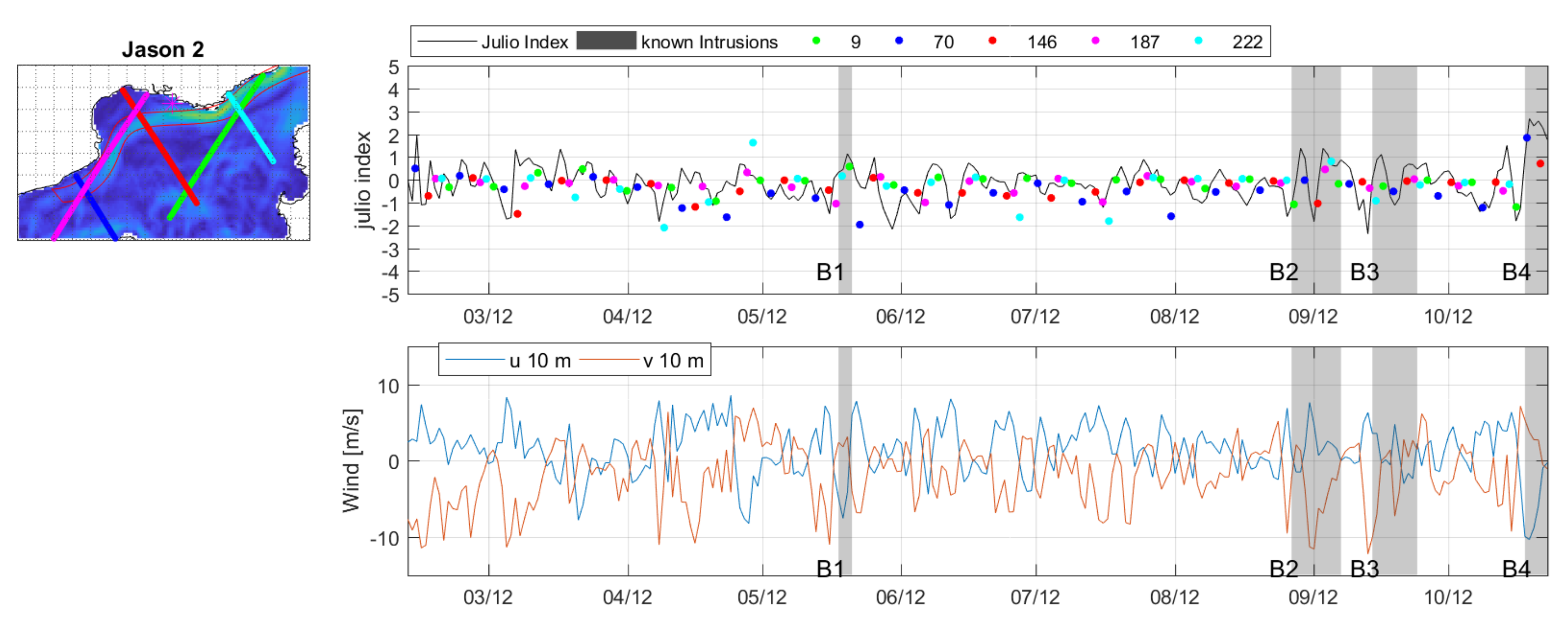
The regressive RFA has then been applied to altimetry data, together with mean horizontal winds at the JULIO location obtained from ECMWF reanalysis ERA Interim. The input SLAs have been corrected by applying equation (6). The resulting predicted fluxes have been compared to the measured Jind. The time series of the results of the regressive RFA are shown in Figure 4, Figure 5 and Figure 6. To help the interpretation, the results have been separated in 3 groups: Jason 2, Saral/Altika descending and ascending tracks. The times corresponding to well-known intrusion events (see BPO16) are highlighted in gray, and labeled with a B and a progressive number. The intrusions relative to the JULIO observations not included in BPO16 are labeled with a “N” (for the supplementary intrusions detected in this paper). Moreover, Table 3 shows some statistics for each intrusion, such as the wind data (main wind direction and mean amplitude during each intrusion), as well as the maximum Jind and . The predicted fluxes that are substantially underestimated have been highlighted (light gray if is lesser than 1 and dark gray if it is lesser than 0.5). The intrusion events that were particularly short in time (1–2 days) are labeled with a “*”. As general rules, we consider that an intrusion has been correctly identified if the maximum during the intrusion is higher than 1 and we estimate to have a false alarm any time is higher than 1 without the presence of an intrusion. It is worth remembering that in BPO16, a Jind higher than 1 has been used to define intrusions. As both and Jind are standardized variables, the threshold of 1 for both indexes corresponds to value greater than 1 standard deviation with respect to the mean value.
An accurate analysis of the results in Figure 4, Figure 5 and Figure 6 and Table 3 has been carried out considering three main periods:
Figure 4, 12 February 2012–23 October 2012: Jason 2 data are available (Saral/Altika was not launched yet). The estimated flux follows pretty well the progress of the Jind time series with some overestimations (e.g., from 27 September to 10 October 2012, the mean bias is 0.94). In general, four main intrusions have been observed in this period (B1–B4). B1 and B4 are characterized by Southerlies meridional winds and have been correctly represented by the algorithm. B2, between the end of August and the beginning of September, is characterized by a northwesterly wind and is well reproduced by the regression algorithm (note the red dot from track 146 that correctly predicts a strong negative flux while the rest of the intrusion is well characterized by positive and strong fluxes). Finally, B3, in mid-September, shows a complex trend in the flux (positive at first and then negative). This flux is not well predicted by the regression algorithm, probably due to the highly variable wind forcing of that period. A false alarm is visible along track 222 on April 28.
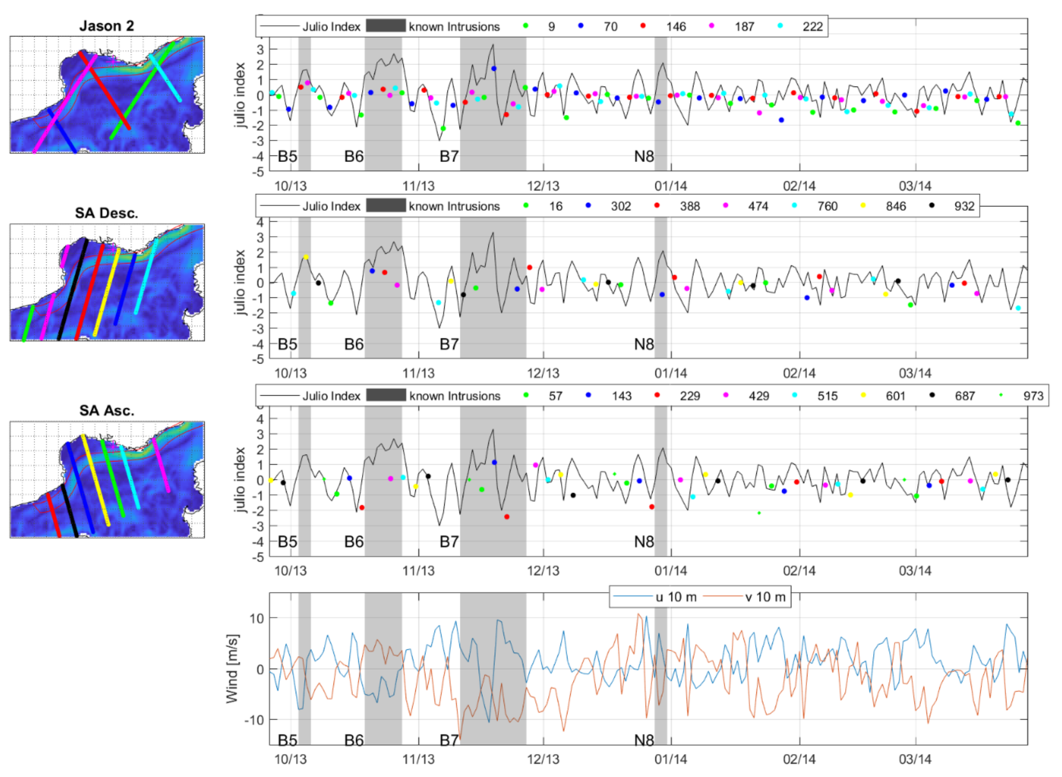
Figure 5, 26 September 2013–28 March 2014 both Jason 2 and Saral/Altika measurements were available. Overall, follows very well the Jind time series. During this period four main intrusions have been observed. Two of them (B5, N8) are very short and quite weak. Although B5 is associated with Southerly meridional wind and has been correctly detected by both Jason 2 and Saral/Altika, N8 happened with a Southerly meridional wind and has been detected neither by Jason 2 nor by Saral/Altika. The other two intrusions (B6 and B7) are both very intense and quite long. B6 is associated with northwesterly wind and B7 with Southerly wind. Both satellites have correctly detected both intrusions even if B6 flux is underestimated w.r.t. JULIO.
Figure 6, 17 July 2014–10 April 2015: The 5 main intrusions N9–N13 have all been detected by both altimeters, even if they both underestimate the flux intensity. The very strong negative fluxes (between N10–N11 and between N12 and N13) have not been detected and Jason 2, RFA produced two false alarms (track 9 on 30 September 2014, and track 70 on 30 November 2014).
Some general comments on the results can be drawn. Table 3 shows the maximum flux during each intrusion as observed by Jason 2 and Saral/Altika, compared with the maximum JULIO index at the same period. Jason 2 and Saral/Altika provide similar performance in intrusion detection, if we consider an intrusion as detected when the maximum of the predicted standardized flux is above 1. Overall, the application of the algorithm to both satellites gives very satisfying results: 93% of the intrusions have been correctly identified, i.e, only the intrusion N8 in Table 3 has been substantially underestimated by both Jason 2 and Saral/Altika, with a very small number of false alarms (3 overall, one of which is evident in the Jason 2 track 70 RFA around 30 November 2014). Therefore, the application of the regression algorithm to real data replicates well Jind. However the detection capability of the algorithm is not as good when the intrusion is brief (1–2 days; for example N8) or occurs during complex wind conditions, especially with abrupt changes in the direction of the horizontal winds (for example B3).
4. Discussion
This work consists of the application of a machine learning technique to the detection of current intrusions into the Gulf of Lion.
The RFA for the detection of current intrusions is based on two main inputs: the Sea Level Anomalies from altimetry datasets and horizontal winds from a global meteorological model. It is well known that the geostrophic component of currents in the direction perpendicular to the track can be derived from altimetry data. Therefore, the information available from altimetry for the detection of current intrusions (i.e., the current anomaly) has two limitations: first, it accounts only for the geostrophic component of the current and, secondly, only in one direction (perpendicular to the satellite track) that may or may not be coincident (or even similar) to the main direction of the current intrusion. Furthermore, the presence of strong winds shall affect the relative importance of the geostrophic and ageostrophic currents, augmenting the ageostrophic component. This shall be particularly true in case of north-westerly winds (see the discussion in BPO16). Nevertheless, recent work combining ocean glider, coastal radar, vessel survey and in-situ and numerical meteorological data, stated that the Northern current is mostly zonal and in geostrophic balance even at the surface [23]. Moreover, the altimetry data showing the larger importance for the training of the algorithm is the SLA very near the coast. Unfortunately, it is exactly where the altimetry technology is more problematic, due to the potential contamination from land of the radar waveform and, secondarily of the radiometer signal. Fortunately, in the last 10 years altimetry has made great progress in the quality of measurements in the coastal region, due to the development of targeted re-tracker, and of corrections and data filtering specific to the coastal areas. This progress opens new paths for several applications in coastal areas and this work can be considered as an example. The paramount importance, in this work, of the use of X-TRACK data has to be highlighted, as any attempt to replicate these results with Geophysical Data Records (GDRs products),provided by space agencies, was unsuccessful. The main reasons for this failure were the absence of altimetry data in proximity of the coast and the important noise level in the immediate surrounding areas.
The choice of the second input used by the RFA, the horizontal winds, is based on several physically robust studies on the dynamics of coastal circulation processes in the Gulf of Lion (see BPO16, [5,24] and included references) and on a long series of experimental oceanographic campaigns in this area. The importance in the RFA algorithm of the main horizontal wind direction in the previous 1–2 days confirms the results of BPO16, where two main mechanisms were identified for the generation of current intrusions, as detailed in the introduction.
It must be highlighted that some of the limitations of the algorithm are due to discrepancies in the training and testing dataset: the training dataset is based on daily simulations, while the testing one is based on instantaneous observations from satellite altimetry. Moreover, the test is based on Jind, a standardized mean current projected in a certain direction that is a point-based measurement, while the algorithm predicts the volume flux through a relatively large surface. Some limitations are probably also related to the physics of the problem as the altimetry-based sea level anomaly is directly linked to the geostrophic current anomaly, while the volume flux (or the mean current on JULIO) is related to geostrophic and ageostrophic component of the currents. Last, but not least, the observations that play a major role in the training of the algorithm are the ones very near the coast, in the region where the altimetric signal is strongly affected by the presence of land.
Despite the small geographical area of application of this algorithm, the methodology is easily replicable in other areas of the world. The only need is a long time series of ocean model simulations.
In this study, the validation of the algorithm has benefited from the availability of high-quality measures from the bottom-moored ADCP of the JULIO site. This availability has been fundamental for testing the algorithm. However, the choice of the satellite usable for this study was limited from the measure time series available from JULIO. In particular, only Jason 2 and Saral/Altika data have been used, while more recent series of measurements could be compared with a RFA tuned with more recent high resolution SAR altimeter such as CryoSat-2 [25] and Sentinel 3 A/B [26] as well as the coming Sentinel 6 [27], and the wide-swath altimetry missions (SWOT [28]), which should allow the monitoring of current anomalies in two directions. Hence, this work opens the door to multiple future interesting applications.
5. Conclusions
This work shows the results of a random forest algorithm applied to SLA from coastal altimetry observations (X-TRACK). The algorithm has been trained on 10 years of model simulations from the SYMPHONIE model, to predict intrusions of the Northern Current in the eastern part of the GoL. These intrusions are quantified by the volume flux that crosses the 200m isobath in a well-defined area. The algorithm replicates the simulated volume flux very well, i.e., the correlation between the predicted and the reference flux is higher than 0.96 and the ARMSE is lower than 19% of the interquartile range. Sensitivity analysis in the training of the algorithm evidenced the high importance of the horizontal wind forcing, especially 1–2 days before the event, as well as the contribution of the Sea Level Anomalies very near the coast.
As shown, the application of the algorithm to satellite-altimetry-based SLAs has given very satisfying results. A detailed comparison with in situ data, from the JULIO mooring, showed that 93% of the intrusions have been correctly identified, with only a few false alarms. The capability of the algorithm to predict the volume flux weakens when the horizontal wind conditions change rapidly. By the way, it is important to highlight that the use of a dataset specifically developed for coastal areas was a necessary condition for the realization of this experiment.
This study has given very promising results; however many benefits should be gained in the future by using the new generation high resolution SAR altimeters such as CryoSat-2 [25] and Sentinel 3 [26] as well as the forthcoming Sentinel 6 [27] and the wide-swath altimetry missions (SWOT, [28]) and the Ka/Ku-band Copernicus Polar Ice and Snow Topography Altimeter (CRISTAL) high-priority candidate mission ([29]), which should strongly improve our capability to monitor relatively small-scale coastal currents.
Author Contributions
Conceptualization, D.C., M.M., A.A.P., A.M.D. and J.B.; Data curation, D.C.; Formal analysis, D.C.; Methodology, D.C., M.M., A.A.P., A.M.D. and J.B.; Software, D.C.; Supervision, A.A.P. and A.M.D.; Writing—original draft, D.C.; Writing—review & editing, D.C., M.M., A.A.P., A.M.D. and J.B. All authors have read and agreed to the published version of the manuscript.
Funding
This research was funded by the European Space Agency (ESA) WP 3327-6 of the IDEAS+ contract NO 4000111304/14/I-AM.
Acknowledgments
The data for this study are publicly available for the users: The X-TRACK altimetry dataset (doi: 10.6096/CTOH_X-TRACK_2017_02) is distributed by the aviso.altimetry.fr portal. The ECMWF ERA Interim dataset is available from the ECMWF website (https://www.ecmwf.int/en/forecasts/datasets/reanalysis-datasets/era-interim). The JULIO measurements can be downloaded from https://erddap.osupytheas.fr/erddap/griddap. The SYMPHONIE model dataset (doi: 10.1007/s10236-017-1040-9) is available at https://dataset.osupytheas.fr/geonetwork/srv/eng/catalog.search;jsessionid=D92B7B8889A3A6F7976E8E0E6BD40A49#/metadata/b3b81334-62ec-4e1d-9103-09bfcec11b62. A.M.D. and A.A.P. are supported by the CNES oceanography program.
Conflicts of Interest
The authors declare no conflict of interest. The funders had no role in the design of the study; in the collection, analyses, or interpretation of data; in the writing of the manuscript, or in the decision to publish the results.
References
- Millot, C. Mesoscale and seasonal variabilities of the circulation in the western Mediterranean. Dyn. Atmos. Oceans 1991, 15, 179–214. [Google Scholar] [CrossRef]
- Ross, O.N.; Fraysse, M.; Pinazo, C.; Pairaud, I. Impact of an intrusion by the Northern Current on the biogeochemistry in the eastern Gulf of Lion, NW Mediterranean. Estuar. Coast. Shelf Sci. 2016, 170, 1–9. [Google Scholar] [CrossRef] [Green Version]
- Petrenko, A.A. Variability of circulation features in the Gulf of Lion NW Mediterranean Sea. Importance of inertial currents. Oceanol. Acta 2003, 26, 323–338. [Google Scholar] [CrossRef] [Green Version]
- Petrenko, A.; Leredde, Y.; Marsaleix, P. Circulation in a stratified and wind-forced Gulf of Lions, NW Mediterranean Sea: in situ and modeling data. Cont. Shelf Res. 2005, 25, 7–27. [Google Scholar] [CrossRef]
- Gatti, J. Intrusions du Courant Nord Méditerranéen sur la Partie est du Plateau Continental du Golfe du Lion. Ph.D. Thesis, Aix-Marseille 2, Marseille, France, 2008. Available online: http://www.theses.fr/2008AIX22095 (accessed on 2 November 2020).
- Barrier, N.; Petrenko, A.A.; Ourmières, Y. Strong intrusions of the Northern Mediterranean Current on the eastern Gulf of Lion: insights from in-situ observations and high resolution numerical modelling. Ocean Dyn. 2016, 66, 313–327. [Google Scholar] [CrossRef] [Green Version]
- Lagerloef, G.S.E.; Mitchum, G.T.; Lukas, R.B.; Niiler, P.P. Tropical Pacific near-surface currents estimated from altimeter, wind, and drifter data. J. Geophys. Res. Space Phys. 1999, 104, 23313–23326. [Google Scholar] [CrossRef]
- Vignudelli, S.; Birol, F.; Benveniste, J.; Fu, L.-L.; Picot, N.; Raynal, M.; Roinard, H. Satellite Altimetry Measurements of Sea Level in the Coastal Zone. Surv. Geophys. 2019, 40, 1319–1349. [Google Scholar] [CrossRef]
- Bouffard, J.; Vignudelli, S.; Herrmann, M.; Lyard, F.; Marsaleix, P.; Ménard, Y.; Cipollini, P. Comparison of Ocean Dynamics with a Regional Circulation Model and Improved Altimetry in the North-Western Mediterranean. Terr. Atmos. Ocean Sci. 2008, 19, 117–133. [Google Scholar] [CrossRef] [Green Version]
- Bouffard, J.; Roblou, L.; Birol, F.; Pascual, A.; Fenoglio-Marc, L.; Cancet, M.; Morrow, R.; Ménard, Y. Introduction and Assessment of Improved Coastal Altimetry Strategies: Case Study over the Northwestern Mediterranean Sea. In Coastal Altimetry; Springer: Berlin/Heidelberg, Germany, 2011; pp. 297–330. [Google Scholar] [CrossRef]
- Meloni, M.; Bouffard, J.; Doglioli, A.M.; Petrenko, A.A.; Valladeau, G. Toward science-oriented validations of coastal altimetry: Application to the Ligurian Sea. Remote Sens. Environ. 2019, 224, 275–288. [Google Scholar] [CrossRef] [Green Version]
- Lee, S.; Im, J.; Kim, J.; Kim, M.; Shin, M.; Kim, H.-C.; Quackenbush, L.J. Arctic Sea Ice Thickness Estimation from CryoSat-2 Satellite Data Using Machine Learning-Based Lead Detection. Remote Sens. 2016, 8, 698. [Google Scholar] [CrossRef] [Green Version]
- Shen, X.; Zhang, J.; Zhang, X.; Meng, J.; Ke, C. Sea Ice Classification Using Cryosat-2 Altimeter Data by Optimal Classifier–Feature Assembly. IEEE Geosci. Remote Sens. Lett. 2017, 14, 1948–1952. [Google Scholar] [CrossRef]
- Ashkezari, M.D.; Hill, C.N.; Follett, C.N.; Forget, G.; Follows, M.J. Oceanic eddy detection and lifetime forecast using machine learning methods. Geophys. Res. Lett. 2016, 43, 12–234. [Google Scholar] [CrossRef] [Green Version]
- Birol, F.; Fuller, N.; Lyard, F.; Cancet, M.; Niño, F.; Delebecque, C.; Fleury, S.; Toublanc, F.; Melet, A.; Saraceno, M.; et al. Coastal applications from nadir altimetry: Example of the X-TRACK regional products. Adv. Space Res. 2017, 59, 936–953. [Google Scholar] [CrossRef]
- Leger, F.; Birol, F.; Nino, F.; Passaro, M.; Marti, F.; Cazenave, A. X-Track/Ales Regional Altimeter Product for Coastal Application: Toward a New Multi-Mission Altimetry Product at High Resolution. In Proceedings of the IGARSS 2019—2019 IEEE International Geoscience and Remote Sensing Symposium, Yokohama, Japan, 28 July–2 August 2019; pp. 8271–8274. [Google Scholar]
- Estournel, C.; Kondrachoff, V.; Marsaleix, P.; Vehil, R. The plume of the Rhone: numerical simulation and remote sensing. Cont. Shelf Res. 1997, 17, 899–924. [Google Scholar] [CrossRef]
- Marsaleix, P.; Auclair, F.; Estournel, C. Considerations on Open Boundary Conditions for Regional and Coastal Ocean Models. J. Atmos. Ocean. Technol. 2006, 23, 1604–1613. [Google Scholar] [CrossRef]
- Hu, Z.Y.; Doglioli, A.M.; Petrenko, A.A.; Marsaleix, P.; DeKeyser, I. Numerical simulations of eddies in the Gulf of Lion. Ocean Model. 2009, 28, 203–208. [Google Scholar] [CrossRef]
- Breiman, L. Random Forests. Mach. Learn. 2001, 45, 5–32. [Google Scholar] [CrossRef] [Green Version]
- Zhang, C.; Ma, Y. (Eds.) Ensemble Machine Learning: Methods and Applications; Springer: Berlin, Germany, 2012. [Google Scholar]
- Belgiu, M.; Drăguţ, L. Random forest in remote sensing: A review of applications and future directions. ISPRS J. Photogramm. Remote Sens. 2016, 114, 24–31. [Google Scholar] [CrossRef]
- Berta, M.; Bellomo, L.; Griffa, A.; Magaldi, M.G.; Molcard, A.; Mantovani, C.; Gasparini, G.P.; Marmain, J.; Vetrano, A.; Béguery, L.; et al. Wind-induced variability in the Northern Current (northwestern Mediterranean Sea) as depicted by a multi-platform observing system. Ocean Sci. 2018, 14, 689–710. [Google Scholar] [CrossRef] [Green Version]
- Petrenko, A.A.; Doglioli, A.M.; Nencioli, F.; Kersalé, M.; Hu, Z.; D’Ovidio, F. A review of the LATEX project: Mesoscale to submesoscale processes in a coastal environment. Ocean Dyn. 2017, 67, 513–533. [Google Scholar] [CrossRef] [Green Version]
- Parrinello, T.; Shepherd, A.; Bouffard, J.; Badessi, S.; Casal, T.; Davidson, M.; Fornari, M.; Maestroni, E.; Scagliola, M. CryoSat: ESA’s ice mission—Eight years in space. Adv. Space Res. 2018, 62, 1178–1190. [Google Scholar] [CrossRef]
- Donlon, C.J.; Berruti, B.; Buongiorno, A.; Ferreira, M.-H.; Féménias, P.; Frerick, J.; Goryl, P.; Klein, U.; Laur, H.; Mavrocordatos, C.; et al. The Global Monitoring for Environment and Security (GMES) Sentinel-3 mission. Remote Sens. Environ. 2012, 120, 37–57. [Google Scholar] [CrossRef]
- Scharroo, R.; Bonekamp, H.; Ponsard, C.; Parisot, F.; Von Engeln, A.; Tahtadjiev, M.; De Vriendt, K.; Montagner, F. Jason continuity of services: Continuing the Jason altimeter data records as Copernicus Sentinel-6. Ocean Sci. 2016, 12, 471–479. [Google Scholar] [CrossRef] [Green Version]
- Fu, L.L.; Alsdorf, D.; Morrow, R.; Rodriguez, E.; Mognard, N. SWOT: The Surface Water and Ocean Topography Mission: Wide-Swath Altimetric Elevation on Earth; Jet Propulsion Laboratory, National Aeronautics and Space Administration: Pasadena, CA, USA, 2012. [Google Scholar]
- Kern, M.; Cullen, R.; Berruti, B.; Bouffard, J.; Casal, T.; Drinkwater, M.R.; Gabriele, A.; Lecuyot, A.; Ludwig, M.; Midthassel, R.; et al. The Copernicus Polar Ice and Snow Topography Altimeter (CRISTAL) high-priority candidate mission. Cryosphere 2020, 14, 2235–2251. [Google Scholar] [CrossRef]
Figure 1.
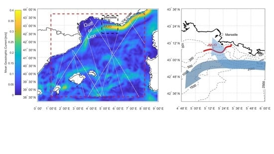
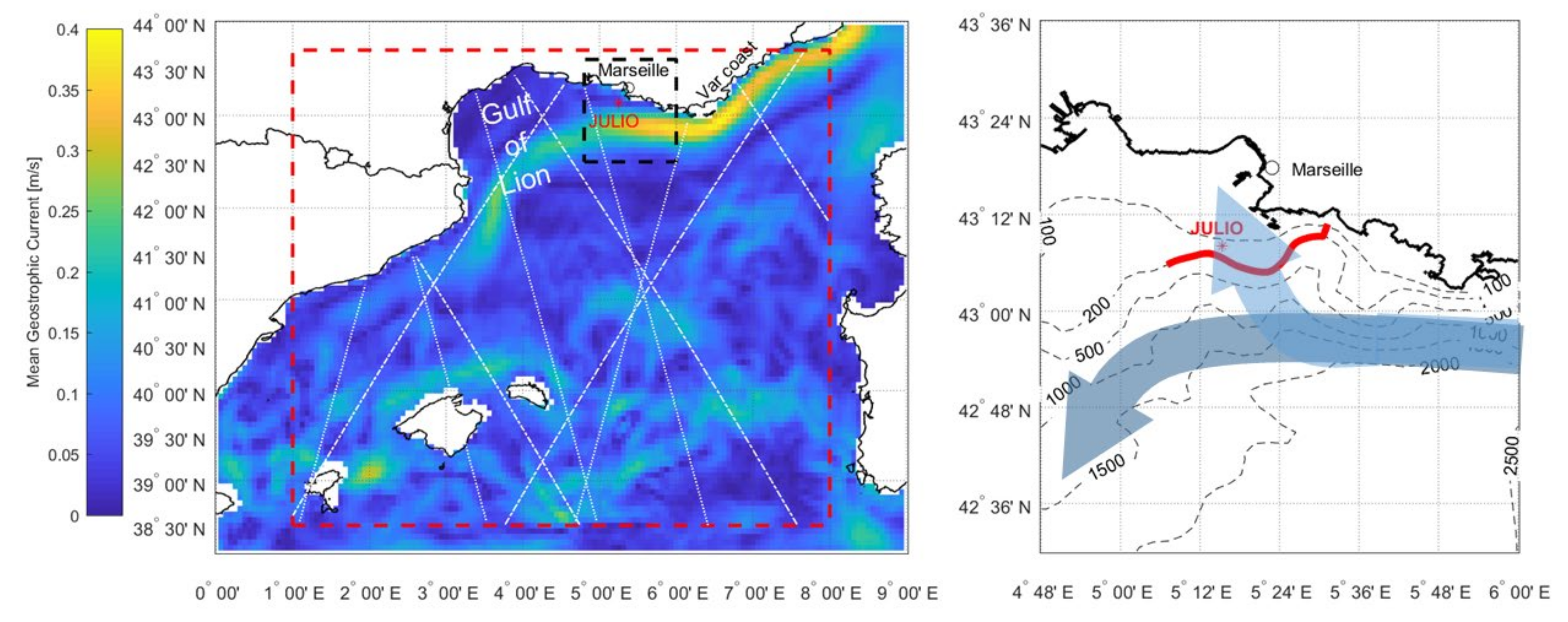
On the left panel the study area (red square), together with the mean geostrophic current intensity, from the numerical simulations, highlighting the mean position of the Northern Current. The Jason 2 and Saral/Altika tracks in the study area are also shown as dashed and dotted lines respectively. On the right panel a zoom on eastern Gulf of Lion, showing the 200 m isobath surface (in red) used to define the volume flux, with the position of the JULIO current meter; a dark blue arrow shows the mean NC position and a light blue one the main direction of current intrusions.
Figure 1.
On the left panel the study area (red square), together with the mean geostrophic current intensity, from the numerical simulations, highlighting the mean position of the Northern Current. The Jason 2 and Saral/Altika tracks in the study area are also shown as dashed and dotted lines respectively. On the right panel a zoom on eastern Gulf of Lion, showing the 200 m isobath surface (in red) used to define the volume flux, with the position of the JULIO current meter; a dark blue arrow shows the mean NC position and a light blue one the main direction of current intrusions.

Figure 2.
Example of the feature importance analysis in the random forest algorithm (left panel); and application to simulated data (i.e., Volume flux is shown in Sverdrup, 1 Sv = 106 m3/s) for Saral/Altika track 302.
Figure 2.
Example of the feature importance analysis in the random forest algorithm (left panel); and application to simulated data (i.e., Volume flux is shown in Sverdrup, 1 Sv = 106 m3/s) for Saral/Altika track 302.

Figure 3.
Analysis of the sensitivity of the RFA error (in terms of ARMSE%) to the distance from JULIO. Jason 2 and Saral/Altika ARMSE% obtained in the training as function of the distance from JULIO are shown, differentiating the ascending and descending passes.
Figure 3.
Analysis of the sensitivity of the RFA error (in terms of ARMSE%) to the distance from JULIO. Jason 2 and Saral/Altika ARMSE% obtained in the training as function of the distance from JULIO are shown, differentiating the ascending and descending passes.

Figure 4.
Results of the application of the regressive random forest algorithm to observational data, (Jason 2). Right panel shows the map of the tracks considered for the period 12 February–23 October 2012, colors refer to the tracks number in the legend on the right panel. On the right panel the comparison between the JULIO index (Jind) (as a black line) and the predicted normalized Flux (), for each track (color dots with reference to the upper legend) is shown in the upper panel. The Lower panel show the corresponding mean daily horizontal winds. In both panels, the periods corresponding to well-known intrusion events are highlighted in gray.

Figure 5.
Results of the application of the regressive random forest algorithm to observational data, (Jason 2 and Saral/Altika). Right panel shows the map of the tracks considered for the period 26 September–31 December 2013, and the corresponding comparison between Jind and for from top to bottom, Jason 2, Saral/Altika Descending and Ascending tracks, please note the color code (same for maps and comparison panels) as specified in the legend. The lower panel shows the mean daily horizontal winds. The periods corresponding to well-known intrusion events are highlighted in gray in all panels.

Figure 6.
Same as Figure 5 for the period 17 July 2014–10 April 2015.
Figure 6.
Same as Figure 5 for the period 17 July 2014–10 April 2015.


Table 1.
List of the chosen altimeter tracks. For each track the satellite identifier, the track number, the minimum distance from JULIO, the length of the track segment used in this study, the minimum distance of the track from the northern Mediterranean Coast and the orientation of the track (A for Ascending, D for Descending) are reported.
| Satellite | Track # | Distance from JULIO [km] | Track Length [km] | Min. Distance from Coast {km] | Ascending/Descending |
|---|---|---|---|---|---|
| J2 | 9 | 138 | 418 | 3.5 | D |
| J2 | 70 | 280 | 203 | 12.3 | A |
| J2 | 146 | 79 | 332 | 5.8 | A |
| J2 | 187 | 61 | 609 | 4.9 | D |
| J2 | 222 | 119 | 197 | 6.5 | A |
| SA | 16 | 205 | 98 | 10.6 | D |
| SA | 57 | 33 | 91 | 2.4 | A |
| SA | 143 | 147 | 91 | 4.2 | A |
| SA | 229 | 261 | 90 | 8.2 | A |
| SA | 302 | 77 | 90 | 7.6 | D |
| SA | 388 | 37 | 82 | 7.9 | D |
| SA | 429 | 136 | 90 | 6.6 | A |
| SA | 474 | 149 | 90 | 4.8 | D |
| SA | 515 | 23 | 90 | 4.6 | A |
| SA | 601 | 90 | 98 | 3.6 | A |
| SA | 687 | 204 | 90 | 4.7 | A |
| SA | 760 | 134 | 91 | 6.3 | D |
| SA | 846 | 20 | 90 | 9.1 | D |
| SA | 932 | 93 | 81 | 1.5 | D |
| SA | 973 | 83 | 90 | 4.3 | A |
Table 2.
Statistical scores and fit parameters for each track in the simulated application of the Random Forests algorithm.
Table 2.
Statistical scores and fit parameters for each track in the simulated application of the Random Forests algorithm.
| Satellite | Track # | Correlation | Slope | Offset [Sv] | ARMSE [1] [Sv] | ARMSE% [1] |
|---|---|---|---|---|---|---|
| J2 | 9 | 0.968 | 0.772 | 1.26E–01 | 2.20E–02 | 16.8% |
| J2 | 70 | 0.963 | 0.753 | 1.34E–02 | 2,.33E–02 | 17.7% |
| J2 | 146 | 0.968 | 0.781 | 1.19E–02 | 2.24E–02 | 17.0% |
| J2 | 187 | 0.973 | 0.795 | 1.12E–02 | 2.08E–02 | 15.9% |
| J2 | 222 | 0.960 | 0.752 | 1.37E–02 | 2.42E–02 | 18.5% |
| SA | 16 | 0.961 | 0.755 | 1.33E–02 | 2.39E–02 | 18.2% |
| SA | 57 | 0.970 | 0.789 | 1.18E–02 | 2.19E–02 | 16.6% |
| SA | 143 | 0.964 | 0.765 | 1.29E–02 | 2,.34E–02 | 17.8% |
| SA | 229 | 0,.958 | 0.743 | 1.41E–02 | 2.45E–02 | 18.6% |
| SA | 302 | 0.964 | 0.756 | 1.34E–02 | 2.29E–02 | 17.4% |
| SA | 388 | 0.967 | 0.767 | 1.27E–02 | 2.23E–02 | 16.9% |
| SA | 429 | 0.959 | 0.745 | 1.43E–02 | 2.41E–02 | 18.4% |
| SA | 474 | 0.967 | 0.775 | 1.23E–02 | 2.25E–02 | 17.1% |
| SA | 515 | 0.967 | 0.778 | 1.22E–02 | 2.27E–02 | 17.2% |
| SA | 601 | 0.968 | 0,780 | 1.20E–02 | 2,23E–02 | 16.9% |
| SA | 687 | 0.961 | 0.751 | 1.34E–02 | 2.36E–02 | 18.0% |
| SA | 760 | 0.964 | 0.756 | 1.34E–02 | 2.30E–02 | 17.5% |
| SA | 846 | 0.968 | 0.764 | 1.28E–02 | 2.17E–02 | 16.5% |
| SA | 932 | 0.969 | 0.785 | 1.13E–02 | 2.21E–02 | 16.8% |
| SA | 973 | 0.961 | 0.756 | 1.32E–02 | 2.40E–02 | 18.3% |
[1] ARMSE stands for Adjusted Root Mean Squared Error, it corresponds to the mean of the absolute value of the residuals of the fit, or in other terms to the RMSE adjusted by the slope and bias parameters, where bias and offset have been removed from the predicted values. ARMSE% is the ARMSE divided by the interquartile range of the flux, expressed in percentage.
Table 3.
List of intrusions with the main wind direction, the maximum Jind during the intrusion, the maximum normalized flux from Jason 2 and Saral/Altika and the mean horizontal wind during the intrusion. Intrusions signed with a * are very fast (1–2 days).
Table 3.
List of intrusions with the main wind direction, the maximum Jind during the intrusion, the maximum normalized flux from Jason 2 and Saral/Altika and the mean horizontal wind during the intrusion. Intrusions signed with a * are very fast (1–2 days).
| Intrusion | Wind Dir. | Max Jind | Mean U Wind | Mean V Wind | ||
|---|---|---|---|---|---|---|
| B1 | SE | 1.14 | 1.15 | −1.88 | 0.31 | |
| B2 | SE–NW | 1.38 | 1.11 | 1.81 | −4.16 | |
| B3 | NW–S NW–SE | 1.11 | 0.90 | 0.37 | −0.88 | |
| B4 | SE | 2.68 | 2.49 | −5.27 | 1.53 | |
| B5 | SE | 1.62 | 2.16 | 2.21 | −0.80 | −2.54 |
| B6 | SE | 2.67 | 1.16 | 1.21 | −3.60 | 3.44 |
| B7 | NW–E–NW | 3.29 | 1.96 | 2.12 | 1.48 | −6.98 |
| N8 * | NW | 2.08 | 0.34 | 0.55 | 1.33 | −1.15 |
| N9 | NW–SE | 1.81 | 2.15 | 0.89 | −2.95 | 1.26 |
| N10 | S | 2.41 | 1.43 | 1.06 | −1.74 | 3.67 |
| N11 | NE–SE–S | 2.37 | 1.45 | 1.23 | −0.86 | −1.47 |
| N12 | NW–S | 2.50 | 0.97 | 0.28 | −0.11 | 1.64 |
| N13 | SE | 2.20 | 2.53 | 1.77 | −5.28 | 3.11 |
Publisher’s Note: MDPI stays neutral with regard to jurisdictional claims in published maps and institutional affiliations. |
© 2020 by the authors. Licensee MDPI, Basel, Switzerland. This article is an open access article distributed under the terms and conditions of the Creative Commons Attribution (CC BY) license (http://creativecommons.org/licenses/by/4.0/).
Share and Cite
MDPI and ACS Style
Casella, D.; Meloni, M.; Petrenko, A.A.; Doglioli, A.M.; Bouffard, J. Coastal Current Intrusions from Satellite Altimetry. Remote Sens. 2020, 12, 3686. https://doi.org/10.3390/rs12223686
AMA Style
Casella D, Meloni M, Petrenko AA, Doglioli AM, Bouffard J. Coastal Current Intrusions from Satellite Altimetry. Remote Sensing. 2020; 12(22):3686. https://doi.org/10.3390/rs12223686
Chicago/Turabian StyleCasella, Daniele, Marco Meloni, Anne A. Petrenko, Andrea M. Doglioli, and Jerome Bouffard. 2020. "Coastal Current Intrusions from Satellite Altimetry" Remote Sensing 12, no. 22: 3686. https://doi.org/10.3390/rs12223686
Note that from the first issue of 2016, this journal uses article numbers instead of page numbers. See further details here.