Novel Ensemble of Multivariate Adaptive Regression Spline with Spatial Logistic Regression and Boosted Regression Tree for Gully Erosion Susceptibility

Abstract

The extreme form of land degradation through different forms of erosion is one of the major problems in sub-tropical monsoon dominated region. The formation and development of gullies is the dominant form or active process of erosion in this region. So, identification of erosion prone regions is necessary for escaping this type of situation and maintaining the correspondence between different spheres of the environment. The major goal of this study is to evaluate the gully erosion susceptibility in the rugged topography of the Hinglo River Basin of eastern India, which ultimately contributes to sustainable land management practices. Due to the nature of data instability, the weakness of the classifier andthe ability to handle data, the accuracy of a single method is not very high. Thus, in this study, a novel resampling algorithm was considered to increase the robustness of the classifier and its accuracy. Gully erosion susceptibility maps have been prepared using boosted regression trees (BRT), multivariate adaptive regression spline (MARS) and spatial logistic regression (SLR) with proposed resampling techniques. The re-sampling algorithm was able to increase the efficiency of all predicted models by improving the nature of the classifier. Each variable in the gully inventory map was randomly allocated with 5-fold cross validation, 10-fold cross validation, bootstrap and optimism bootstrap, while each consisted of 30% of the database. The ensemble model was tested using 70% and validated with the other 30% using the K-fold cross validation (CV) method to evaluate the influence of the random selection of training and validation database. Here, all resampling methods are associated with higher accuracy, but SLR bootstrap optimism is more optimal than any other methods according to its robust nature. The AUC values of BRT optimism bootstrap, MARS optimism bootstrap and SLR optimism bootstrap are 87.40%, 90.40% and 90.60%, respectively. According to the SLR optimism bootstrap, the 107,771 km² (27.51%) area of this region is associated with a very high to high susceptible to gully erosion. This potential developmental area of the gully was found primarily in the Hinglo River Basin, where lateral exposure was mainly observed with scarce vegetation. The outcome of this work can help policy-makers to implement remedial measures to minimize the damage caused by erosion of the gully.

1. Introduction

Soil erosion is a threat to the environment through various forms of erosion, such as sheet, rill, gully, ravine and which finally becomes part of the badland’s topography [1,2,3]. Gullies (0.5 m deep and more than 100 m wide) are formed after the complete process of rill erosion and before the starting stage of a ravine [4,5]. The world suffers from severe soil-related issues, such as loss of fertility and soil quality, and this erosion does in fact have limitations on land use. On-site and off-site environmental problems sometimes cause social or economic losses [2,3,6]. Water moves eroded soil towards rivers, where it reduces the depth of the river and reservoir, causes sediment loss and reduces agricultural productivity. In gully erosion, the top soil of the land is transported away by water and becomes a major source of sediment in rivers. Walling (1998) and May et al.(2005) argued that when soil particles retain less strength than wind, water, and glacier power, soil erosion (rill formation) occurs on the Earth’s surface [7,8]. Soil erosion is considered as a disaster because of its association with several issues such as land degradation, less agricultural productivity and surface quality and quantity, all of which are inversely related to human and environmental health. This type of phenomenon causes desertification, groundwater pollution, flooding and a decline in soil fertility. In order to achieve the objective of sustainable development in modern times, land-use planners, engineers, farmers and the general public are likely to prevent soil loss.

Asia has the highest soil erosion with an annual soil erosion rate of 29.95 tons per hectare due to land degradation. Das (1985) stated that in India, 38% of the total geographical area is subjected to serious erosion. The Ministry of Agriculture, Government of India, published in 1980 that 53% of India’s geographical area has been affected by land degradation in general and soil erosion in particular. According to the information in World Soil Erosion and Conservation (1994), in India, more than 70% of the population is dependent on the agricultural system and 3.7 million hectares of agricultural land suffer from fertility losses [9,10]. The loss of nutrients in the soil causes a number of losses in cereal, oilseed and pulse production, equivalent to USD 2.51 billion [11].

Soil erosion and land degradation are common in the eastern part of India because of prevalent flash floods and the high intensity of rainfall during the monsoon season.

The literature shows that over the last 40 years, one third of the world’s agricultural land has been severely affected by soil erosion, and this process continues [12]. Various studies have provided several suggestions for mitigation strategies of gully erosion. Among them, many researchers argued that the presence of vegetation could reduce gully head cuts and the development of the gully [13,14,15,16]. Land use and land cover change are strongly related to gully influences and controls the topographic threshold condition [13,17]. On the other hand, the root characteristics are capable of increasing soil resistance, and the presence of vegetation in the gully area has a direct effect on soil [18]. Increased root density, size and species may increase head cuts and soil tensile strength in the river bank as indicated by different researchers whoinformed that root related parameters have also been used to determine the gully erosion model [19,20,21]. Although gully erosion is a common type of water erosion, many related factors have made it complex, such as slope, elevation, aspect, plan curvature, profile curvature, stream power index (SPI), distance to river, topographical wetness index (TWI), rainfall, drainage density, surface runoff, organic matter, soil texture, soil moisture, lithology, lineament, distance to road, land use and land cover (LULC), and normalized difference vegetation index (NDVI) [22,23].

In recent times, machine learning (ML) algorithms have been widely used for the spatial prediction of gully erosion [24,25,26]. Based on different causes, land use assessment not only helps to evaluate the resource, but also helps to categorize the risk zone from high to low [27]. Although topographic, geomorphological, geological, hydrological and soil characteristics play an important role in identifying vulnerable areas, they sometimes become insufficient. Chorley (1969) stated that the hydro-geomorphological parameters have a good predictable capacity to establish basin or catchment gully zones. A large number of geo-morphometric parameters were used with statistical techniques and resulted in a logical and systemic output. The Geographic Information System (GIS) environment has made research work more valuable by handling large databases.The GIS considers all factors to determine the occurrence of gully erosion and may be used in the data processing system. Various machine learning, artificial intelligence based, statistical and other models based on the GIS have been used to assess gully susceptibility in a number of literature reviews, such as logistic regression [28,29,30], random forest [25], multivariate adaptive regression spline (MARS) [31], frequency ratio [32], artificial neural network [33] and support vector machine [26,34]. Various physical-based methods have also been used to estimate the amount of erosion from gullies such as the condensed real-time model(CREAMS), which is conducted by runoff and erosion from agricultural management; the ephemeral gully erosion model (EGEM); and the water erosion prediction project (WEPP). In the present study, boosted regression tree (BRT), machine learning model (MARS) and statistical approach (SLR) were used to predict gully areas.

Current research focuses on assessing the impact of different geo-environmental factors on gully erosion susceptibility and identifying the vulnerable regions. All the data were processed and validated by using machine learning and statistical model based approaches. There are two types of approaches to the occurrence of gully erosion which have been identified considering the existing literature. The relationship with gully erosion and physical conditions is based on a training dataset that will finally be validated through different model and field based information. Various factors, such as topographical, hydrological, climatic, anthropogenic and morphometric factors, have influenced soil erosion. The overall objectives are: 1. Identify the major geo-environmental causes of gully erosion in the study region. 2. Evaluate changes in the land area and their environmental impact 3. Establish and locate gully prone areas in a variety of models (BRT, MARS, and SLR) 4. Finally, produce a map of the susceptibility of gully erosion with management of erosion and control planning. The main contributing aspect of this paper is the development of the most optimal model considering different appropriate resampling algorithms.

2. Study Area

We have focused on the Hinglo river basin, a tributary and fifth order stream of Ajoy River in eastern India. Gully erosion is getting acute due to soil erosion by water through poor drainage systems and over unprotected land surfaces in this river basin. The basin area covers 444.308 km² and the length of this river is 65 km. The Hinglo River basin is located between 23°42′7″ N to 24°0′56″ N and 86°59’32” E to 87°23′31″ E (Figure 1). Granitic rock of the Pleistocene age was found in the upper catchment area, while Barakar formations and ironstone shale formed in lower catchment area [35]. The groundwater potentiality increased towards the east, where older alluvium deposition also increased over time. Mukherjee et al. (2007) stated groundwater table variation depends on seasonal fluctuations [36]. In this region, ferruginous processes made the soil characteristics different and produced a reddish type soil which is called laterite. The north-western part is characterized by physical and chemical weathering, mass wasting, laterization, the red weathered zone and formation of duricrust (a hard layer of minerals developed at or close the soil surface) (Figure 2). The south-eastern part of this region has physiographic features with an alluvial plain. The direction of the slope of this river basin is north to east. The Hinglo River is divided between two states of India (Jharkhand and West Bengal). Originating from the spring of the Jamtara district of Jharkhand, it enters into West Bengal and covers the Birbhum district and finally merges with the Ajoy River near Palashdanga. The climatic characteristics of the area are dominated by the north-eastern monsoon and the south-western monsoon. It is under subtropical climatic categories where the summer is hot and dry, and the winter is dry. The rainfall (80%) is due to the south-western monsoon and the forest land is quite low. The annual rainfall is 1316 mm and the elevation ranges from 0 to 289 mt. The National Atlas and Thematic Mapping Organization (NATMO) (2001) recognized the soil textural class of the area as sand, clay, loam, sandy loam, loam and fine loam. By completing a geological survey, we identified different geological segments such as quartzite, alluvium, shale and granite gneiss. During the field survey, the erosion of the gully was mainly found in the upper and middle regions where the slope is steeper to gentle. The Hinglo River covered the Chhotanagpur Plateau in the West Bengal Plain and, therefore, the erosion distribution of the gully is heterogeneous. In the upper and middle parts, people are converting their own land into agricultural land, building construction profiles and clearing the forest, which in turn affects the soil and forms gullies. Preparing the gully profile, we found the ‘V’ shaped gully in the upper segment and the U shaped gully in the middle section due to the deposition process.

3. Materials and Methods

3.1. Database

Various databases were considered in this study. Detailed information about the databases is shown in

Table 1. Database and its sources.

	Parameters	Data Type	Sources	Data Details
1	Elevation	Raster grid	ALOS PALSAR DEM, (Alaska Satellite Facility)	12.5 m spatial resolution
2	Slope gradient (degree)	Raster grid	ALOS PALSAR DEM, (Alaska Satellite Facility)	12.5 m spatial resolution
3	Slope aspect	Raster grid	ALOS PALSAR DEM, (Alaska Satellite Facility)	12.5 m spatial resolution
4	Plan Curvature	Raster grid	ALOS PALSAR DEM, (Alaska Satellite Facility)	12.5 m spatial resolution
5	Profile curvature	Raster grid	ALOS PALSAR DEM, (Alaska Satellite Facility)	12.5 m spatial resolution
6	Geology (detailed lithology and deposits)	Line, point and polygon coverage	Geological Survey of India (http://bhukosh.gsi.gov.in/Bhukosh/Public)	Different unit of lithology
7	Geomorphology	Line, point and polygon coverage	Geological Survey of India (http://bhukosh.gsi.gov.in/Bhukosh/Public)	Different spatial geomorphological unit
8	Soil texture	polygon coverage	NBSS&LUP, SAMETI (Jharkhand)	Textural class
9	Drainage density	Polygon coverage buffer	ALOS PALSAR DEM, (Alaska Satellite Facility)	12.5 m spatial resolution
10	Stream Power Index (SPI)	Raster grid	ALOS PALSAR DEM, (Alaska Satellite Facility)	12.5 m spatial resolution
11	Drainage Proximity	Polygon coverage buffer	ALOS PALSAR DEM, (Alaska Satellite Facility)	12.5 m spatial resolution
12	Topographical Wetness Index (TWI)	Raster grid	ALOS PALSAR DEM, (Alaska Satellite Facility)	12.5 m spatial resolution
13	Land use and land cover (LULC)	Spatial/Raster grid	Sentinel 2A (European Space Agency)	10 m spatial resolution
14	Normalized difference vegetation index (NDVI)	Spatial/Raster grid	Sentinel 2A (European Space Agency)	10 m spatial resolution
15	Soil Moisture	netCDF file format	Simulation model by IIT Kharagpur, India [37]	Monthly soil moisture data
16	Distance from Road	Spatial/Raster grid, Polygon coverage buffer	Topographical map, Google earth, Sentinel 2A (European Space Agency)	10 m spatial resolution
17	Distance from Lineament	Line, point and polygon coverage	Geological Survey of India	Different shape of lineament
18	Slope length and steepness factor	Raster grid	ALOS PALSAR DEM, (Alaska Satellite Facility)	12.5 m spatial resolution
19	Rainfall and runoff erosivity factor	Point wise collected rainfall data in storm period	Primary observed data	Raster
20	Soil erodibility factor	Estimated from the collected samples	Primary observed data	Raster

.

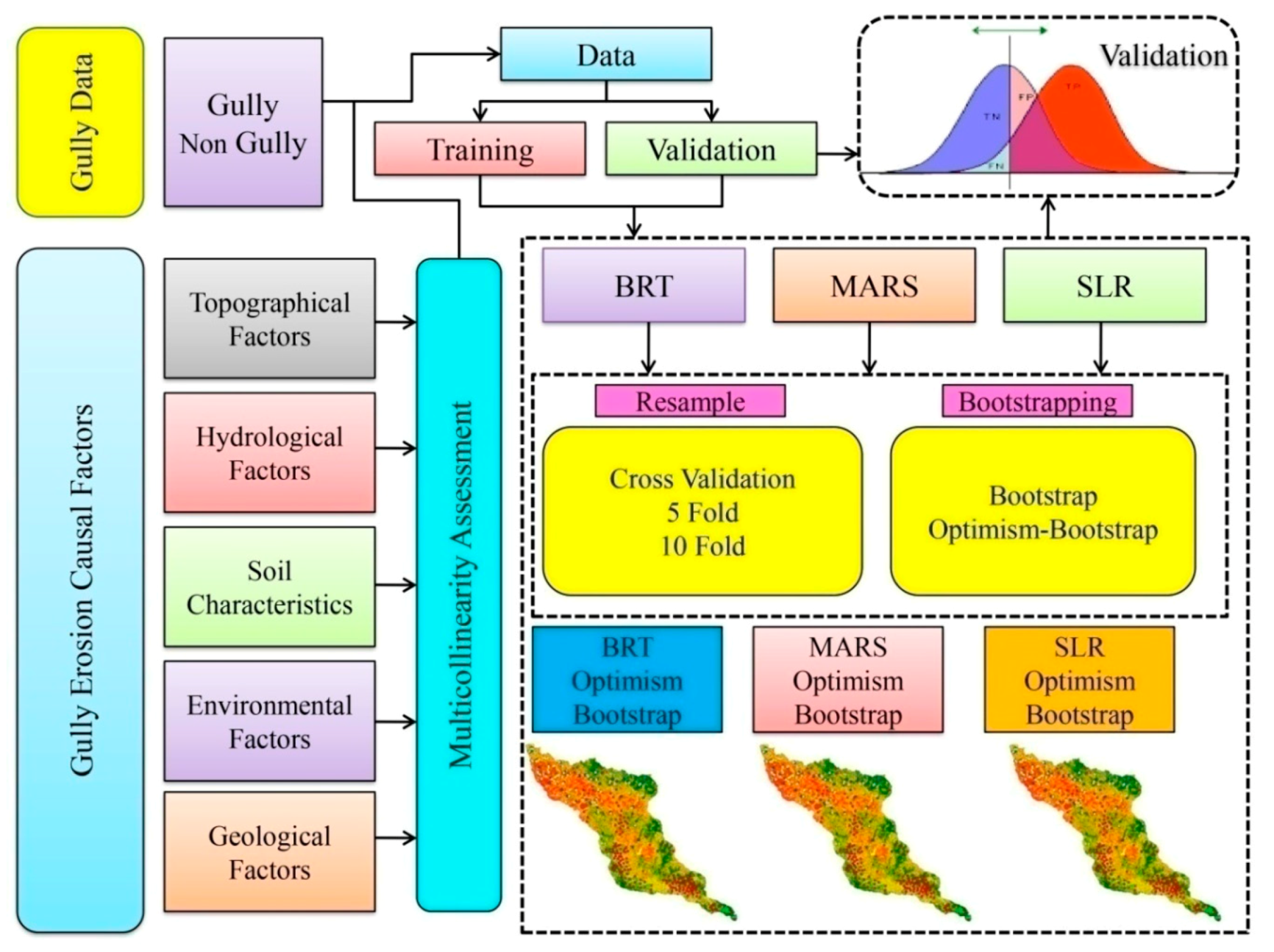
3.2. Data Source and Framework of Methodology

In this research, different geo-environmental data were used, such as topographical parameters, hydrological, soils, geological and environmental factors. The whole procedures of current research work have been presented infour steps. These are: 1. Create an inventory map of the gully using satellite data and information from field observation. 2. Based on geo-environmental causative factors, prepare the gully erosion susceptibility map of the Hinglo River basin by applying different approaches. 3. Use ArcGIS 10.3 to prepare the thematic layers and create the gully erosion susceptibility map for the study area.

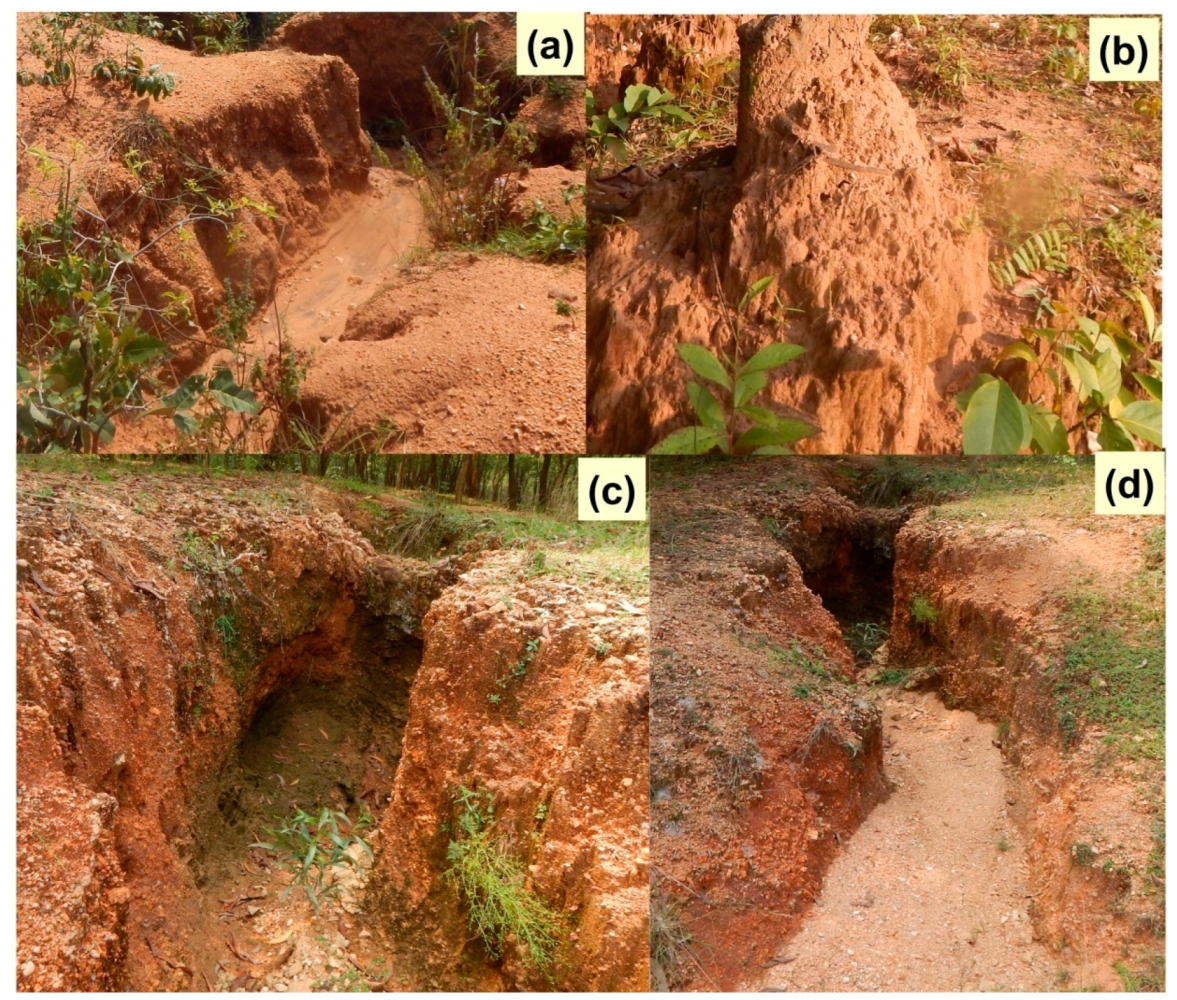
3.3. Gully Inventory Map (GIM)

The locations of the gullies were identified during the field survey using a hand-held GPS, Google Earth images, aerial photos (1:10,000) and a topographical map (1:50,000). We considered the training to be an input process and this map validates the models as a result. Among the 100 gully inventory points, 70% were used as inputs and 30% were used as validations, which were randomly divided. Not only the gully area, but also the non-gully area is shown in this inventory map.

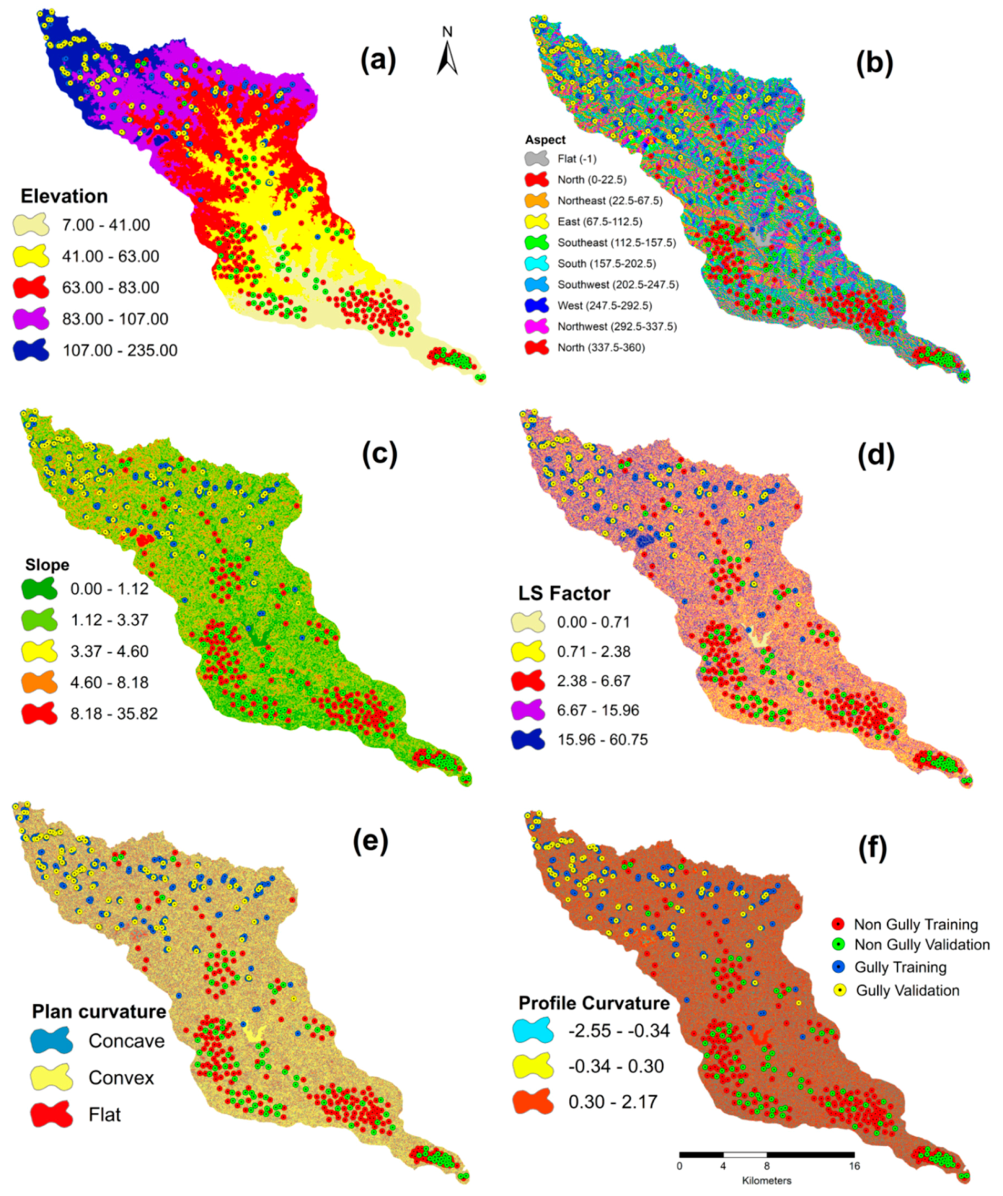
3.4. Conditioning Factors

A literature review shows us different geo-environmental factors that cause gully erosion [38,39]. Therefore, each and every factor must be very prominent. These geo-environmental factors were classified into such categories:

3.4.1. Topographical

Topography plays a major role in developing gullies. Gómez-Gutiérrez et al. (2015) stated topographic features control the drainage network, erosive power and water velocity [40]. Six topographic parameters were counted to develop the gully erosion susceptibility map, such as slope, elevation, aspect, plan curvature, profile curvature and slope length and steepness (LS) factor (Figure 3). These were extracted from ALOS (Advanced land observing satellite) PALSAR (Phased array L-band synthetic aperture radar) DEM (Digital elevation model) with 12.5 mt resolution. The detailed methods for estimating the LS factor are as follows:

$$\begin{gathered} LS={\left(FlowAccumulation\times cellsize/22.13\right)}^{0.4} \\ \times \left(Sin\left[Slopegrid\times 0.01745\right]/0.0896, 1.4) \times 1.4\right) \end{gathered}$$

(1)

$$\begin{gathered} LS=Pow\left(\left[FlowAccumulationGrid\right]\times 12.5/22.13,0.4) \times Pow \left(Sin \left[Slopegrid \\ \times 0.01745\right)/0.0896, 1.4\right)\times 1.4\right) \end{gathered}$$

(2)

where Pow is the Power on the ArcGIS platform, Flow Accumulation is the grid layer of the accumulation of the flow as expressed the number of grid cells, and the cell size is the length of the grid cells. The L and S factors have been estimated from the ALOSPALSAR DEM.

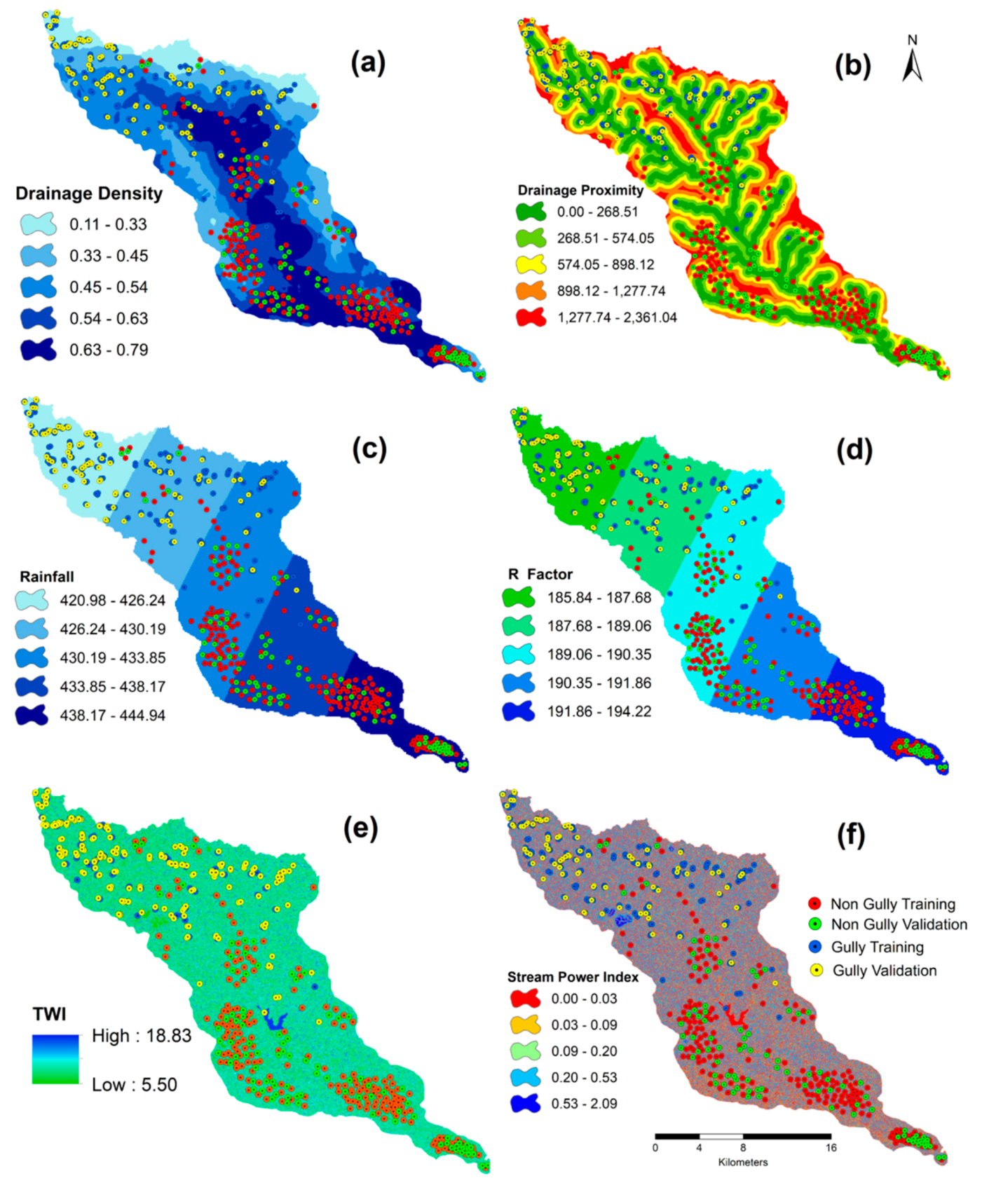
3.4.2. Hydrological Factors

Drainage density, drainage proximity, rainfall, rainfall and runoff erosivity (R) factor, topographical wetness index (TWI) and stream power index (SPI) were considered as hydrological parameters (Figure 4). The drainage density of this region has been estimated from ALOSPALSAR DEM, taking into account 1000 threshold values in the GIS environment. The rationale for selecting this threshold value was based on the previous literature in this region [41]. Apart from this, the estimated drainage network is similar to Google Earth, satellite images and topographic maps (Survey of India). Annual rainfall data were collected from the India Meteorological Department(IMD). The drainage density and stream power index were extracted from the DEM. By forming and developing gullies, the river can extend its own length. The SPI is calculated as follows [42]:

$$SPI=As \times tan \sigma$$

(3)

where As represent total catchment area, σ indicates the slope gradient [43].

TWI has been computed by using the following equation:

$$TWI=Ln\frac{\propto }{tan\beta +C}$$

(4)

where ∝ is the Flow Accumulation β is the Slope and C is the Constant (0.01).

The R factor of this region has been calculated with the help of the following equation [44,45]:

$$R={\displaystyle \sum }_{i=0}^{12}1.735\times {10}^{\left(1.5{\log }_{10}\left(\frac{P_i^2}{P}\right)-0.08188\right)}$$

(5)

where R is the rainfall and runoff erosivity factor and it express in MJ/ha/year.

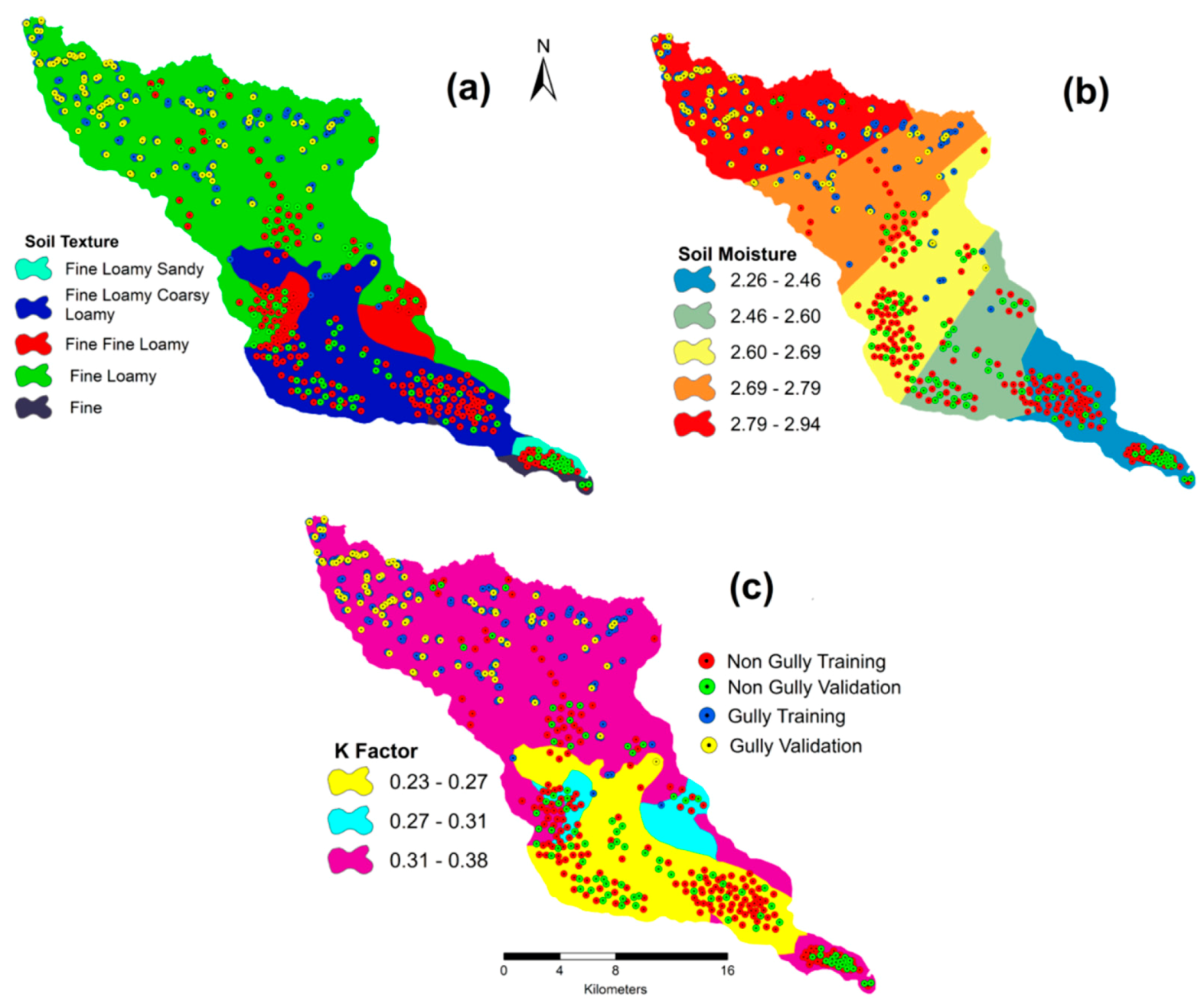
3.4.3. Soil Characteristics

Gully erosion is a type of soil erosion by water, where soil texture, soil depth and soil properties control the erosive capacity of the water (Figure 5), where organic matter, soil moisture and soil texture are considered asthe primary role for creation and development of gullies. TheNational Bureau of Soil Survey and Land Use Planning (NBSS&LUP), State Agriculture Management and Extension Training Institute(SAMETI) and collected soil samples helped to provide the soil erodibility of this region:

$$K=2.1\times 10–6M1.4\times \left(12–OM\right)+0.0325\times \left(P–2\right)+0.025\times \left(S–3\right)$$

(6)

where K is the soil erodibility (ton ha-1 unit of R); M is the (% silt +% very fine sand) (100—% clay); OM is the percentage of organic matter and P is the permeability class; and S = structure class [46].

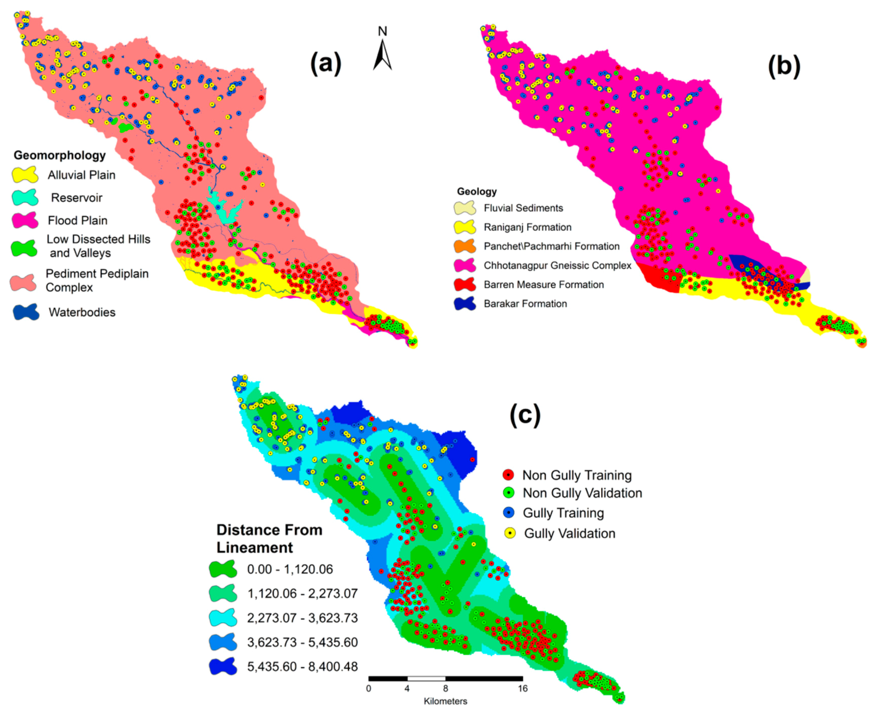
3.4.4. Geological Factors

The thickness of the soil (Figure 6) is dependent on the soil parent material and indirectly controls the formation of the gully. Further information on the geology of the study area was provided by the Geological Survey of India.

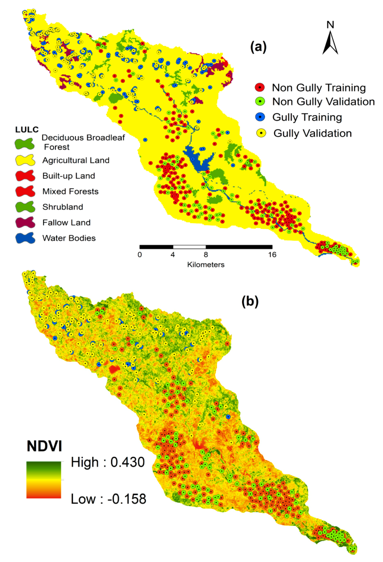
3.4.5. Environmental Factors

Distance from the river, LULC, NDVI and distance from the road affects the surface runoff and is considered as environmental factors (Figure 7). These features were estimated from the topographical map at 1:50,000 and Sentinel 2a satellite image at 10 mt spatial resolution (28 March 2020). The NDVI was estimated using the following equation [47]:

$$NDVI=\frac{NIR-RED}{NIR+RED}.$$

(7)

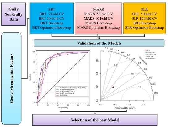
3.5. Methodology Flow Chart for Gully Erosion Susceptibility

The flowchart shows the methodology used in this work. Four parts of this methodology have been included: (1) preparation of data; (2) multi-collinearity assessment using Variance inflation factor (VIF) and tolerance; (3) gully erosion susceptibility modeling by BRT (machine learning), MARS (machine learning ensembles) and SLR (statistical approach) with different resamples (5-fold CV, 10-fold CV, bootstrap and optimism bootstrap) techniques; and (4) process of validation by means of receiver operating characteristics (ROC) curve and different statistical indices (Figure 8).

3.6. Multi-Collinearity Test

Multi-collinearity shows the linear relationship between different variables. This assessment provides the conformity of the application and clarifies the result when statistical approaches are used [22]. It shows the linear dependence of the different independent variables. In each method used, no covariance is passed on to the least absolute shrinkage and selection operator [48]. Cama et al.(2017) stated that the use of VIF with TOL tends to predict co-relationships [49]. VIF connected with TOL, based on the calculation of 1-R^2., where R² is the regressing variable in multivariate regression. The result of VIF associated with TOL varies from less than 0.1 to more than 10 and is strongly multi-collinear.

3.7. Model Used

3.7.1. Boosted Regression Tree

Boosted regression tree (BRT) is a combination of regression tree and boosting [50]. Many decision trees have repeatedly been fitted to the BRT, such as the random forest model, in order to improve the accuracy of the model. There was a difference between the two methods used to construct selected trees in the data. In both techniques, all data were taken randomly for the construction of each new tree. However, the random forest model used the baggage method, which indicated the same probability of subsequent samples being selected for each occurrence. BRT was used as a boosting method, where input data were weighted in the trees. Applying this model, the weights were poorly modeled so that the previous tree was chosen as the new tree. This indicates that the first tree to be fitted to the model will take account of the error and that the tree will become a new tree. In this way, taking the previous tree against a new tree, the model improved its accuracy and became a powerful model. The BRT model considered two parameters to be discussed:

Tree complexity (TC): The number of splits in each tree was controlled by this procedure. The value of 1 showed 1 tree split, which means that the model did not consider interactions between environmental variables. Values greater than 1 or 2 showed two divisions of very high interactions.

Learning rates (LR): This parameter was used to determine the contribution of each tree used to make the model. It was necessary to construct small values of LR in the trees.

The large number of environmental variables compared to observations makes it very useful to strengthen the missing values and the outliers. This model is correlated with sets of independent variables and can accommodate any type of variables such as continuous, categorical, missing and non-independent variables. Important predictor variables enable functions, and their interactions have been identified by BRT and the model has been formed without the assumptions of these interactions or functions [51]. It has been used to solve the problem of regression and classification. It determines the input variables. This is a boosting and optimization technique that boosts the tree’s decision weekly, then prepares the residual, determines the loss of function to calculate it, and shows the difference between the tree’s output and the target values. To minimize the loss of function, boosting the algorithm has added a new tree to each step [51].

$$MCV:sign\left[{\displaystyle \sum }_m^M{a}_m·c_m\left(x\right)\right]$$

(8)

where MCV is the majority vote classification, $a_m:\log \frac{\left(1-r_m\right)}{r_m}$ which $r_m$: is associated to compute the (weighted) misclassification rate, fit classifier c_m to the weighted data. In this equation, recalculate weights $w_i=w\exp (mI\left(y_i\ne c_m\right)$ that initialize weights equal to $w_i=\frac{1}{n}$ for $m=1$ to the next category $c_m$ [52].

3.7.2. Multivariate Adaptive Regression Spline

Friedman stated MARS is an extension of the generalized linear model and is one type of non-parametric regression technique [53]. MARS uses a set of independent variables to predict the value of the output variable and to solve the problem of the regression type. In order to establish a linear or non-linear relationship between dependent and independent variables, this model is partitioned using binary recursive splines. By assessing cut points similar to step functions, the non-linearity aspect of the polynomial regression was captured by the convenient approach provided by multivariate adaptive regression spline (MARS). Predictors have been developed by the procedure, and its individual data points have been developedas a knot and a linear regression model with candidate characteristics. The whole process continues until several knots have been found and a high non-linear pattern has finally been created. These many knots will help tie a good relationship to training data without generalizing new unseen data. In addition, creating a full set of knots makes it easy to remove those knots which do not measure the accuracy significantly. This new removing process, named “Pruning”, uses cross validation with the previous model to find the optimal number of knots. To predict the probabilities in MARS incorporated with logistic regression, we can look at the example of when generalized linear models are incorporated with MARS through the link function. On the other hand, when the underlying form of function is known in the MARS model, non-linear regression and regression have been used to estimate function parameters. Not only that, MARS also estimates functions that have serious limitations on the nature of the functions. As a generalization of recursive partitioning, MARS can better handle non-categorical data. The equation of MARS may be as follows by Quirós et al.(2009) [54]:

$$\max \left(0,x-k\right)or\max \left(0,k-x\right)$$

(9)

where k is the connections and findings one of the dependent components and x is an independent component. Thus, the MARS model is explained as follows:

$$\widehat{y}=\widehat{f}\left(x\right)=\beta +{\displaystyle \sum }_{m=1}^M{\alpha }_m{H}_m\left(x\right)$$

(10)

where y is the function-predicted dependent variable, $\beta$ is a constant, M is the number of terms and $x$ is the categorical variables. $H_m$ is the baseline constant and ${\alpha }_m$, coefficients calculated by reducing the total squared errors.

Craven and Wahba (1978) has stated that to determine the optimal model for MARS, the generalized cross validation method is used [55].

$$GCV=\frac{\frac{1}{N}{{\displaystyle \sum }}_{i=l}^N{\left[y_i-\widehat{f}\left(x_i\right)\right]}^2}{{\left[1-\frac{C\left(H\right)}{N}\right]}^2}$$

(11)

where N is the size of samples and C(H) is the dependent variable which rises with both the amount of base functions (BF) in the model and is determined on the basis of following equation:

$$C\left(H\right)=\left(H+1\right)+dH$$

(12)

where d is the justice for each origin utility is considered in the model and H is the number of essential purposes. The MARS theory does not require a generalization study of the effect between the response variable and the causative parameters. The MARS model is applicable as a machine learning technique by applying specific adaptive developments.

3.7.3. Spatial Logistic Regression

Logistic regression or binary logistic regression is a multivariate regression model where a categorical dependent variable related to many independent variables [56,57]. The predictor variables for regression values predicted the presence and absence of dependent variables [58,59]. The algorithm of logistic regression converted the dependent variables to logit variables by applying maximum likelihood estimation [60]. The merit of LR is that any type of independent variable can be used for the logistic regression algorithm, which means that variables may be normal or categorical [61]. In order to predict the ratio of each independent variable to the dependent variables, the LR coefficient was used for the multivariate model [62]. The factors and the dependent variables are numerical, and the dependent variables must have the nominal data for the LR algorithm. The occurrence of gully erosion depends on a number of pedo-gromorphic and hydrological factors. The forward, backward stepwise and enter logistic regression method have been used in many studies, but the entire method gets the all coefficients of regression. Now, all coefficients of regression were needed for further raster calculation and developed a gully erosion susceptibility map by spatial logistic regression. Statistically, the LR algorithm with the relationship of independent (gully erosion causative factors) and dependent (occurrences of gullies) variables is expressed below as Equations (13) and (14) [61,63].

$$P=\frac{1}{\left(1+e^{-z}\right)}$$

(13)

$$Z= b_0+b_1{x}_{1+}{b}_2{x}_2+\dots +b_n{x}_n$$

(14)

In Equation (13), P is the predicted probability of gully erosion, where the probability value varies from 0 to 1 on anS-shaped curve, and z is the linear combination expressed in the following equation. In Equation (14), b₀ is the constant of the model, b_i (i = 1, 2,…, n) is the slope or coefficients of the LR model, and x_i (i = 1, 2,…, n) is the independent variable. Binary LR is a non-spatial model and there is a spatial auto-correlation between data. As a result, the spatial structure is included in the logistic regression model by changing some expressions. Now, the following modified equation may be used for spatial logistic regression (SLR). In this spatial autocorrelation, three things are important.These are spatial weight matrix (W), spatial autocorrelation parameter (p) and error term obeying a Gaussian distribution (ε). The spatial structure of gully erosion is calculated through Equations (15) to (18) below [64]:

$$W=\left[\begin{array}{ccc}\begin{array}{cc}0& f\left(d_{12}\right)\end{array}& \cdots & f\left(d_{ij}\right)\\ \begin{array}{cc}f\left(d_{21}\right)& 0\end{array}& \dots & f\left(d_{2j}\right)\\ \begin{array}{cc}\begin{array}{c}⋮\\ f\left(d_{i1}\right)\end{array}& \begin{array}{c}⋮\\ f\left(d_{i2}\right)\end{array}\end{array}& \begin{array}{c}\ddots \\ \dots \end{array}& \begin{array}{c}⋮\\ 0\end{array}\end{array}\right]$$

(15)

$$f\left(d_{ij}\right)=\frac{d_{ij}}{{{\displaystyle \sum }}_1^j{d}_{ij}}$$

(16)

$$L=y \ln \frac{\exp \left(a+X\beta +\rho Wy\right)}{1+\exp \left(a+X\beta +\rho Wy\right)}-\left(1-y\right)\ln (1+\exp \left(a+X\beta +\rho Wy\right))$$

(17)

$$Z= b_0+b_1{x}_{1+}{b}_2{x}_2+\dots +b_n{x}_n+ \rho WY+\epsilon$$

(18)

where $\rho WY$ is the spatial structure effect caused by spatial autocorrelation, W is the weight matrix, $f\left(d_{ij}\right)$ is the inverse weighting function expressed as Equation (15),$\epsilon$ is the error term obeying a Gaussian distribution, and L is the integrated nested Laplacian approximation to reduced time during estimation [65]. The statistical software was used to calculate the correlation between the location and erosion of the gully, which affects the coefficient of the factors. The rest of the work on the GIS platform was carried out by the raster calculator, following Equations (15) and (18) to produce an SLR map of gully erosion susceptibility.

3.8. Resampling Methods

Resampling methods are used to draw samples from a dataset repeatedly and to re-assemble a model for each sample in order to learn more about the fitted model. Resampling methods can be costly, as they require repeated output from different N subsets of data using the same statistical method. In order to obtain further information on the model fitted, this method adjusts the model of interest to the samples generated by the training dataset. They provide the estimates of test-set forecast error, the confidence interval, and the bias of our estimates for the parameters. The error of the experiment is the average error resulting from the use of a statistical learning system to evaluate the effects on a sample not used to train the process. On the other hand, the error in training can be conveniently assessed by finding a statistical learning method for the measurements used in training. Various resampling algorithms are available, including: cross validation (CV), leave-one-out cross validation (LOOCV), K-fold cross validation, and bootstrap.

3.8.1. K-Fold Cross Validation

K-fold cross-validation is performed by arbitrarily dividing the result collection into K classes or folds of approximately the same scale. Related to a single-out cross-validation, one of the K-folds is used as a collection of validation, while the other K-folds are used as a collection of checks to calculate the check error for K. The forecast check error for K-fold cross-validation is the sum of all results.

Typical values for K are 5 or 10, since they require fewer calculations than when K is equal to n. Cross-validation can be used both to determine how well a specific statistical learning process performs on recent data and to determine the lowest point in the calculated square mean error curve, which may be helpful in contrasting statistical learning methods or in contrasting different degrees of versatility for a single statistical learning model.

3.8.2. Bootstrap

The bootstrap is a universally applied method used to quantify the uncertainty of a given estimation method or statistical learning process, along with those for which it is difficult to measure the variability. By repeatedly collecting data from the source data set, bootstrap generates a separate dataset. These datasets can be used instead of sampling independent datasets from the target population as a whole. Bootstrap sampling includes anarbitrary selection of substitution inferences, which means that certain findings can be identified numerous times while other observations have not been included [66].

This method is reproduced B times to produce B data sets, Z, Z₁, Z₂, ..., Z_B, which can be used to measure only certain quantities like standard error.

3.9. Validation and Accuracy Assessment

Various statistical methods like sensitivity (TPR), specificity (SPC), precision (PPV), negative predictive value (NPV), false positive rate (FPR), false discovery rate (FDR), false negative rate (FNR), accuracy (ACC), F₁score (F₁)and positive predictive values (PPV) were used [67,68,69,70,71,72,73,74,75,76,77,78] to test the performance of the machine learning models used in the present research. Positive and negative predictive values (PPV and NPV) are the amounts of positive and negative results, respectively, in data and experimental measures, which are true positive and true negative findings. Greater values of these predictive measures suggest higher performance of the models [79].

Sensitivity of the predicted models has been estimated with considering following equation:

$$TPR=\frac{TP}{TP+FN}$$

(19)

where, TP is the true positive and FN is the false negative.

Specificity of this estimation has been worked out with considering the following equation:

$$SPC=\frac{TN}{FP+TN}$$

(20)

where, TN is the true negative, FP is the false positive and TN is the true negative.

PPV is the pixel probability value is classified as a gullying area. The calculation is given bellow:

$$PPV=\frac{TP}{TP+FP}$$

(21)

where, PPV is the positive predictive value, TP is the true positive, FP is the false positive of this estimation.

Negative predictive value has been measured with the help of the following equation:

$$NPV=\frac{TN}{TN+FN}$$

(22)

False positive rate has been estimated with the help of the following equation:

$$FPR=\frac{FP}{FP+FN}$$

(23)

False discovery rate of this estimation has been worked out with the help of the following equation:

$$FDR=\frac{FP}{FP+TP}$$

(24)

where, FDR is the false discovery rate, FP is the false positive and TP is the true positive.

False negative rate of this analysis has been estimated with considering the following equation:

$$FNR=\frac{FN}{FN+TP}$$

(25)

where, FNR is the false negative rate, FN is the false negative and TP is the true positive.

Accuracy of the all predicted models was estimated with the help of the following equation:

$$ACC=\frac{TP+TN}{P+N}$$

(26)

where, ACC is the accuracy, TP is the true positive, TN is the true negative, P is the positive and N is the negative values of this estimation.

F₁ Score has been estimated with the help of the following equation:

$$F_1=\frac{2TP}{2TP+FP+FN}$$

(27)

where, $F_1$ is the harmonic mean of the precision, TP is the true positive, FP is the false positive and FN is the false negative.

Alternatively, the Matthews correlation coefficient (MCC) is a much robust statistical metric that only generates a high scores if the forecast yielded good outcomes in all basic uncertainty matrix groups (TP, FN, TN, and FP), both in comparison to the amount of positive sides and the size of negative aspects in the database:

$$MCC=\frac{\left(\left(TP\times TN\right)-\left(FP\times FN\right)\right)}{\sqrt{\left(\left(TP+FP\right)\times \left(TP+FN\right)\times \left(TN+FP\right)\times \left(TN+FN\right)\right)}}$$

(28)

The AUC of ROC has been estimated with the help of the following method:

$$S_{AUC}={\displaystyle \sum }_{k=1}^n\left(X_{k+1}-X_k\right)\left(S_k+1-S_{k+1}-\frac{S_k}{2}\right)$$

(29)

where, $S_{AUC}$ is the area under curve, $X_k$ is the 1-Specificity and $S_k$ is the Sensitivity of the ROC.

A common instrument for calculating model output is the receiver operating characteristic (ROC). ROC is plotted on the x- and y-axis, depending on the sensitivity and 1-specificity. ROC’s area under curve (AUC) is projected on model efficiency. The statistical principle and the equation of this method are presented in detail in previous studies [80]. Sensitivity (i.e., likelihood of detection) raises the issue of which portion of the gully erosion observed is correctly labeled, and its optimum value is 1. The precision (i.e., negative predictive rate) raises the issue of which part of the non-gully erosion is accurately defined, and its optimum value is 1 [81]. AUC values below 0.6, 0.6–0.7, 07–0.8, 0.8–0.9 and above 0.9 suggest the model’s poor, fair, average, outstanding and very high consistency, respectively. The ROC, which trains data collection, generates model performance and finally tests the suitability of a model. The ROC from the data collection of the evaluation shows the predictive importance of the model and how strong or poor the predictive model is.

4. Results

4.1. Multi-Collinearity Analysis

Analysis of multicollinearity is another factor selection methodology for assessing the "non-independence" of gully erosion conditioning parameters. Due to higher relationships betweenvariables, the projected outcomes can be inaccurate and inconsistent [82]. It is considered as a linear relationship between different independent variables. The TOL and VIF values are ≥0.1 and ≤10, representing optimal multi-collinearity [83]. In the present study, multi-collinearity has been considered when taking into account the VIF and tolerance values for better accuracy of the predicted models and minimizes the error in this perspective. The highest and lowest VIF and TOL values were 1.099 to 3.688 and 0.271 to 0.909, respectively, taking into account 20 gully erosion conditioning factors (

Table 2. Multi-collinearity assessment.

Sl No.	Variables	Variance Inflation Factor (VIF)	Tolerance
1	Elevation	1.944	0.514
2	Aspect	2.949	0.339
3	Slope	1.276	0.643
4	LS Factor	1.498	0.543
5	Plan Curvature	1.890	0.530
6	Profile Curvature	2.025	0.494
7	Drainage Density	1.655	0.604
8	Drainage Proximity	3.107	0.322
9	Rainfall	2.360	0.420
10	R Factor	1.109	0.902
11	TWI	1.919	0.584
12	SPI	3.060	0.330
13	Soil Texture	2.124	0.471
14	Soil Moisture	1.574	0.635
15	K Factor	2.880	0.350
16	Geomorphology	3.688	0.271
17	Geology	1.460	0.685
18	Distance from Lineament	1.099	0.909
19	LULC	2.290	0.437
20	NDVI	2.430	0.410

). It has been shown that there is no problem of multi-collinearity, therefore the factors responsible for the erosion of the gully have been considered in this research. From

Table 3. Predictive capability of head gully erosion models using train and test data.

Models	Resampleing	Type	Sensitivity	Specificity	Precision	Negative Predictive Value	False Positive Rate	False Discovery Rate	False Negative Rate	Accuracy	F1 Score	Matthews Correlation Coefficient
BRT	Non	Training	0.7143	0.5556	0.7895	0.4545	0.4444	0.2105	0.2857	0.6667	0.75	0.2566
		Validation	0.7262	0.5556	0.7922	0.4651	0.4444	0.2078	0.2738	0.675	0.7578	0.2693
	5-fold CV	Training	0.7275	0.5449	0.7912	0.4575	0.4551	0.2088	0.2725	0.6733	0.758	0.2603
		Validation	0.7327	0.5389	0.7872	0.4641	0.4611	0.2128	0.2673	0.6745	0.759	0.2612
	10-fold CV	Training	0.7357	0.5363	0.7883	0.4638	0.4637	0.2117	0.2643	0.6761	0.7611	0.2618
		Validation	0.7392	0.5304	0.7843	0.4683	0.4696	0.2157	0.2608	0.6761	0.7611	0.2609
	Bootstrap	Training	0.7416	0.5249	0.7828	0.468	0.4751	0.2172	0.2584	0.6761	0.7617	0.2585
		Validation	0.7464	0.522	0.782	0.4726	0.478	0.218	0.2536	0.6783	0.7638	0.2614
	Optimism Bootstrap	Training	0.7608	0.5251	0.7891	0.4845	0.4749	0.2109	0.2392	0.6901	0.7747	0.2797
		Validation	0.7692	0.5193	0.7862	0.4947	0.4807	0.2138	0.2308	0.6935	0.7776	0.2847
MARS	Non	Training	0.7156	0.5618	0.7947	0.4545	0.4382	0.2053	0.2844	0.67	0.7531	0.263
		Validation	0.7303	0.5525	0.7907	0.4695	0.4475	0.2093	0.2697	0.6767	0.7593	0.2713
	5-fold CV	Training	0.7322	0.5525	0.7923	0.4695	0.4475	0.2077	0.2678	0.6783	0.7611	0.273
		Validation	0.7329	0.548	0.7949	0.4619	0.452	0.2051	0.2671	0.6783	0.7626	0.2686
	10-fold CV	Training	0.7387	0.5337	0.7893	0.4634	0.4663	0.2107	0.2613	0.6778	0.7632	0.2624
		Validation	0.7422	0.5278	0.7854	0.468	0.4722	0.2146	0.2578	0.6778	0.7632	0.2615
	Bootstrap	Training	0.747	0.5225	0.7864	0.4673	0.4775	0.2136	0.253	0.6801	0.7662	0.2615
		Validation	0.753	0.5196	0.785	0.4745	0.4804	0.215	0.247	0.6829	0.7687	0.2659
	Optimism Bootstrap	Training	0.7632	0.5196	0.7877	0.4844	0.4804	0.2123	0.2368	0.6901	0.7752	0.2773
		Validation	0.7722	0.511	0.7835	0.4947	0.489	0.2165	0.2278	0.6928	0.7778	0.2806
SLR	Non	Training	0.718	0.5618	0.7953	0.4566	0.4382	0.2047	0.282	0.6717	0.7547	0.2655
		Validation	0.731	0.55	0.7912	0.467	0.45	0.2088	0.269	0.6767	0.7599	0.2693
	5-fold CV	Training	0.7346	0.5393	0.7908	0.4615	0.4607	0.2092	0.2654	0.6767	0.7617	0.2629
		Validation	0.7376	0.5367	0.7919	0.4612	0.4633	0.2081	0.2624	0.6783	0.7638	0.2635
	10-fold CV	Training	0.7411	0.5281	0.7879	0.4631	0.4719	0.2121	0.2589	0.6778	0.7638	0.2599
		Validation	0.7435	0.5225	0.7864	0.4627	0.4775	0.2136	0.2565	0.6778	0.7643	0.2574
	Bootstrap	Training	0.7482	0.5169	0.7855	0.4646	0.4831	0.2145	0.2518	0.6795	0.7664	0.2575
		Validation	0.7578	0.514	0.7841	0.4767	0.486	0.2159	0.2422	0.6846	0.7707	0.2662
	Optimism Bootstrap	Training	0.7722	0.5084	0.7854	0.4892	0.4916	0.2146	0.2278	0.693	0.7787	0.2776
		Validation	0.7754	0.5028	0.7845	0.4891	0.4972	0.2149	0.2249	0.6935	0.7798	0.2758

, it can be seen that every selected parameter for gully erosion is independent in nature and the values of VIF and TOL are associated with the permissible limit (values of TOL and VIF are ≥0.1 and ≤10, respectively). Predictions of the coefficient will vary significantly, depending on which independent variables are associated with this model. Coefficients throughout the method differ from significantly optimistic to minor alterations. Multi-collinearity affects the accuracy of the coefficients that also undermine the outcomesof optimal capacity.

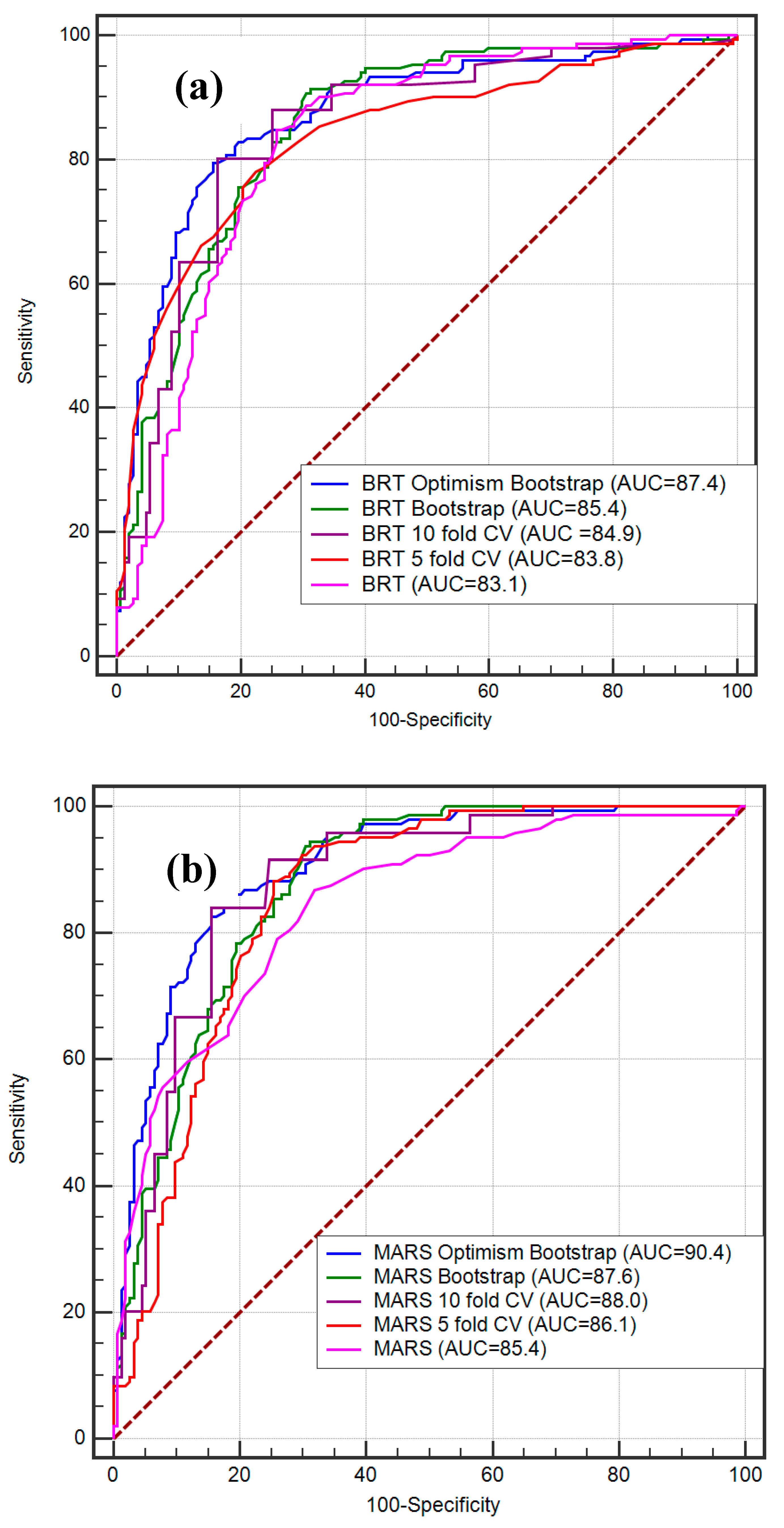
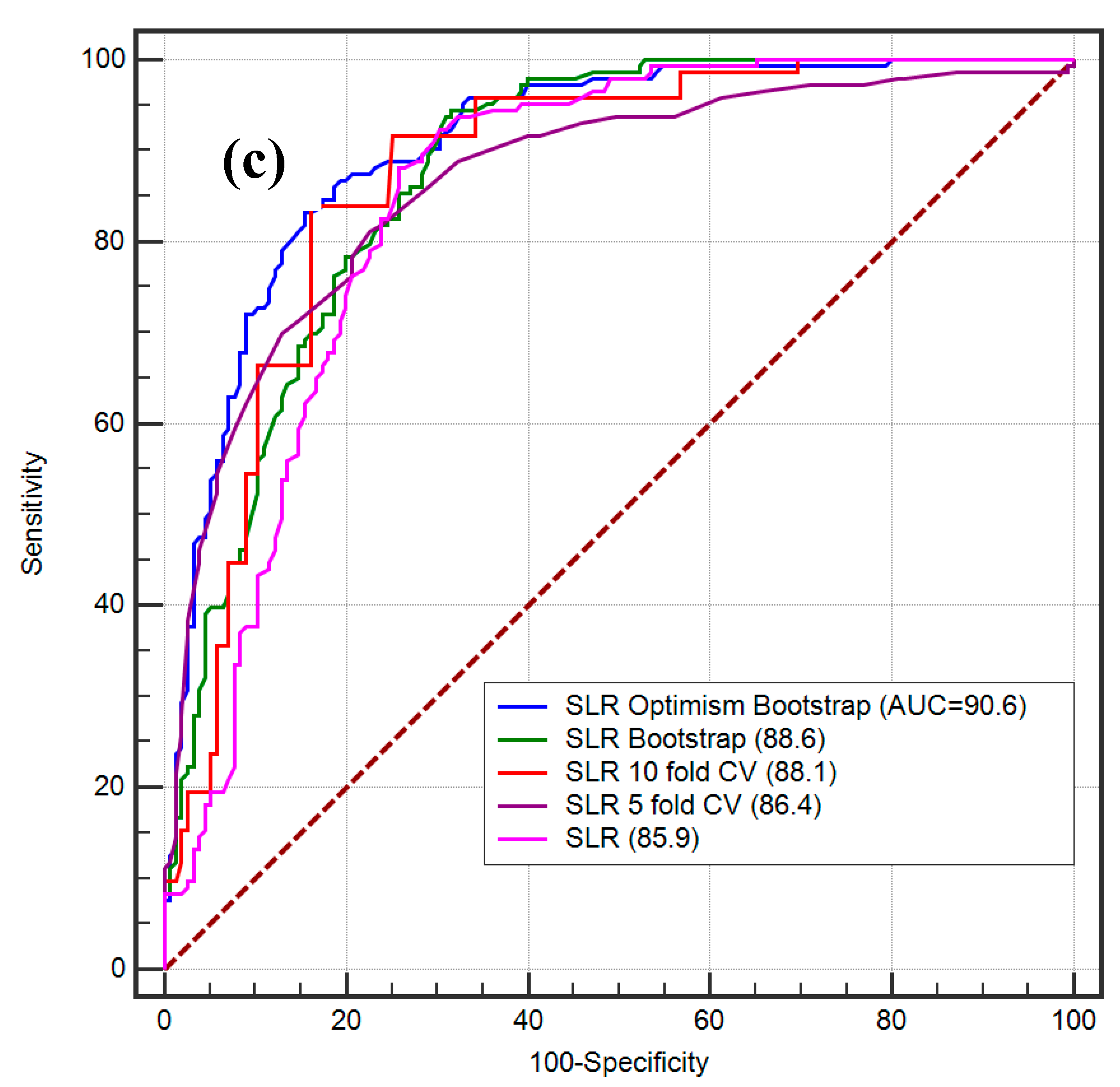
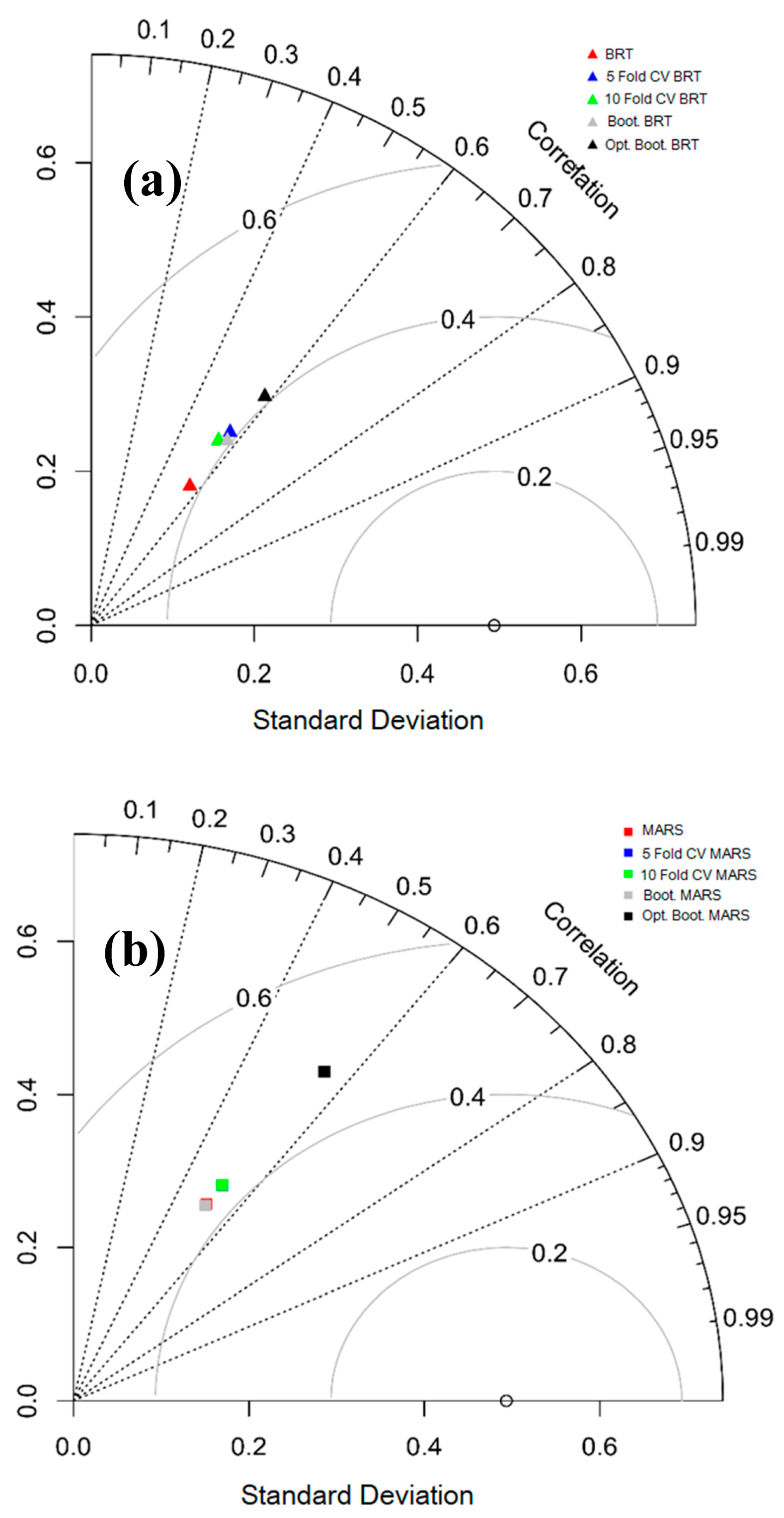
4.2. Validation of the Models

The results of the training data reinforce the gully erosion susceptibility models, while the results of the validation data reflect the optimal evaluation of the final models to fit with the training samples. In this analysis, we present estimation of the statistical index and ROC curve for calculation of the validity of various gully erosion models. Table 3 shows the performance of the various models—BRT, MARS and SLR—with multiple resampling techniques with the help of different statistical outcomes. All statistical findings show that the performance of spatial logistic regression is much better than that of other models. In addition, the findings of gully erosion susceptibility models are validated by performing AUC of ROC on the basis of a database of known gully points. In ROC, the susceptibility models were compared with the gully and non-gully erosion points in the region. The ROC curves have been graphically represented depending on the different threshold reductions using optimistic-class ratios, i.e., true positive rate and false positive rate, to evaluatethe binary classifiers’ dynamic response and associated accuracy. The ROCs for BRT, BRT 5-fold CV, BRT 10-fold CV, BRT bootstrap and BRT optimism bootstrap are 83.1, 83.8, 84.9, 85.4 and 87.4, respectively. The ROC for MARS, MARS 5-fold CV, MARS 10-fold CV, MARS bootstrap and MARS optimism bootstrap are 85.4, 86.1, 88.0, 87.6 and 90.4, respectively. The AUC values of ROC for SLR, SLR 5-fold CV, SLR 10-fold CV, SLR bootstrap and SLR optimism bootstrap are 85.9, 86.4, 88.1, 88.6 and 90.6, respectively. The optimism bootstrap of BRT, MARS and SLR gives better prediction in comparison to the other models. Of them, the SLR model is most optimal according to its predictive capacity (Figure 9).

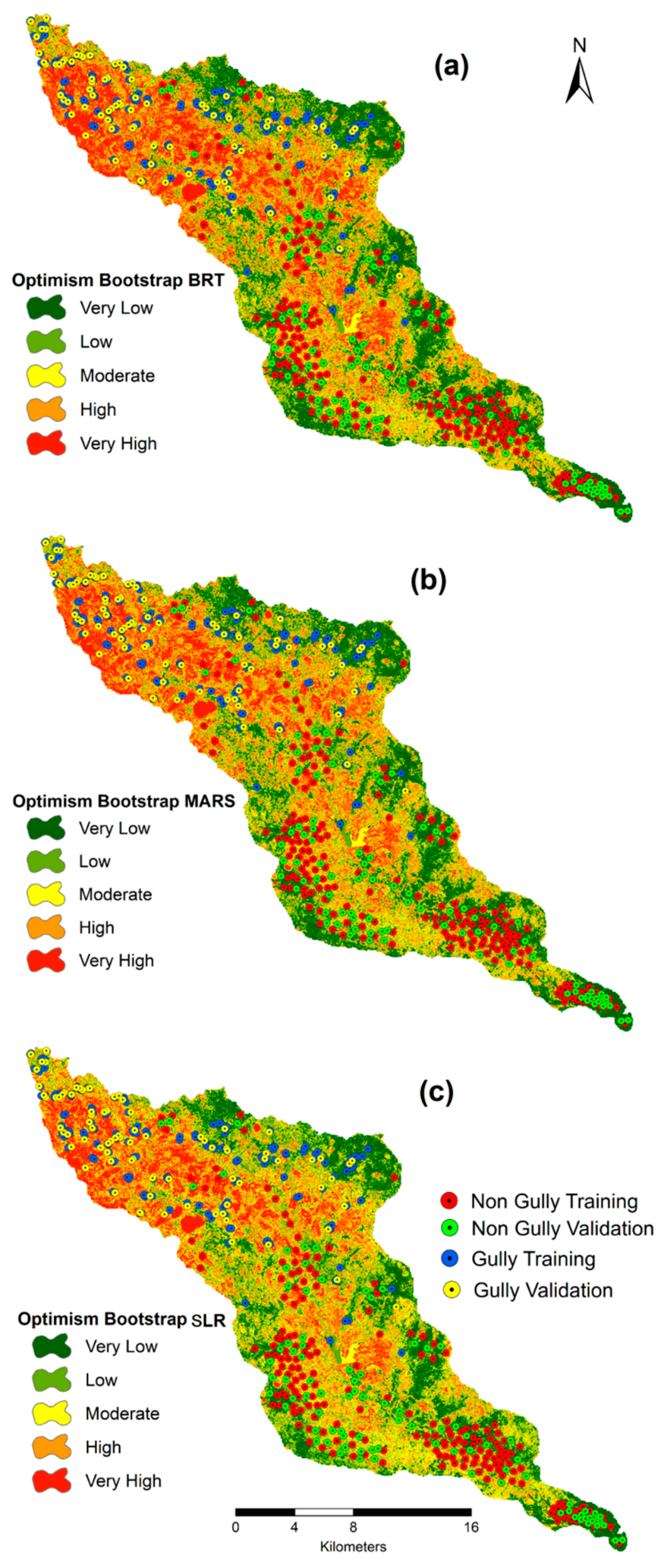
4.3. Gully Erosion Susceptibility Modeling

For a fair evaluation of the estimated susceptibility map, it is essential to find the optimal variables for simulation, as chosen factors in the training dataset depend on each other to create uncertainty in the experiments. In addition, it is important to quantify the predictive efficiency and multi-collinearity of the twenty conditioning parameters chosen when predicting the susceptibility to gully erosion. Thus, calculating the important values of the conditioning parameters is necessary.

Machine learning algorithms such as BRT, MARS and SLR with different resampling approaches (5-fold CV, 10-fold CV, bootstrap and optimism bootstrap) have been used to assess the gully erosion susceptibility (Figure 10). The optimism bootstrap of BRT, MARS and SLR isassociated with better prediction capability than other resampling methods. The optimal capacity of the resampling algorithm has been observed in this research, and the main feature of the resampling algorithm is that it improves the accuracy of the classifier. In the BRT optimism bootstrap model, most of the regions are associated with very low (20.03%), low (28.66%) and medium (25.60%) gully erosion susceptibility where the remaining part of the region isassociated with high (17.55%) and very high (8.16%) susceptible zones.

In the MARS optimism bootstrap model, most of the regions are associated with very low (25.28%), low (21.50%) and medium (25.81%) gully erosion susceptibility where the reaming part of the region isassociated with high (18.79%) and very high (8.62%) susceptible zones (

Table 4. A real percentage of gully erosion susceptible zones.

Susceptibility Class	Models
	Optimism Bootstrap BRT		Optimism Bootstrap MARS		Optimism Bootstrap SLR
	Area (Km2)	Area (%)	Area (Km2)	Area (%)	Area (Km2)	Area (%)
Very Low	101.973	26.030	99.034	25.280	99.465	25.390
Low	80.936	20.660	84.226	21.500	83.756	21.380
Moderate	100.288	25.600	101.111	25.810	100.758	25.720
High	76.587	19.550	73.610	18.790	73.845	18.850
Very High	31.967	8.160	33.769	8.620	33.926	8.660
Total	391.750	100	391.750	100	391.750	100

).

In the SLR optimism bootstrap model, most of the regions are associated with very low (25.39%), low (21.38%) and medium (25.72%) gully erosion susceptibility where the reaming part of the region isassociated with high (18.85%) and very high (8.66%) susceptible zones.

Apart from this, the quality of the predicted models (BRT, MARS and SLR with different resampling techniques) is shown from direct observation with the help of the Taylor diagram (Figure 11). It is capable of drawing graphical findings where a pattern or sets of patterns are closely linked with observations. The relation between different patterns has been identified byconsidering the nature of the correlation, root mean square error (RMSE) and degree of variations. The degree of variations has been estimated byconsidering the standard deviations [84]. The location of an individualpointappearing on the plot evaluates the estimatedpattern of gully erosion susceptibility modelwhich coincides with the observed information. The RMSE-based variation amongthe trends being estimated and observed is proportional to the differencesto the point defined as "observed" on the x-axis. Here, the gray contour indicates the RMSE in the distribution of patterns. The efficiency of optimism bootstrap (SLR optimism bootstrap, MARS optimism bootstrap and BRT optimism bootstrap) is more optimal than other models.

4.4. Importance Value

The selection of the appropriate parameters for modeling is important, as the selected factors depend on each other in the training dataset. Therefore, it is necessary to calculate the predictive capacity and multi-collinearity of the 20 selected conditioning parameters for modeling gully erosion susceptibility, and therefore to calculate the importance values for each conditioning parameter. The findings suggest that the elevation (18.48), drainage density (18.33), LS factor (16.56), R factor (16.06), soil texture (13.52) and rainfall (11.72) are of greater importance where gully erosion occurs, while the other variables, such as aspect (1.60), TWI (1.19), geology (1.46), geomorphology (2.18), distance from lineament (2.33) and others are of lesser importance (

Table 5. Importance values of the gully erosion conditioning factors.

Sl No.	Variables	Importance
1	Elevation	18.48
2	Aspect	1.60
3	Slope	3.47
4	LS Factor	16.56
5	Plan Curvature	4.76
6	Profile Curvature	3.13
7	Drainage Density	6.68
8	Drainage Proximity	18.33
9	Rainfall	11.72
10	R Factor	16.06
11	TWI	1.19
12	SPI	4.92
13	Soil Texture	13.52
14	Soil Moisture	8.16
15	K Factor	6.41
16	Geomorphology	2.18
17	Geology	1.46
18	Distance from Lineament	2.33
19	LULC	3.63
20	NDVI	4.17

). From a partial plot of important variables, it is easy to understand the importance of significant factors and their relationship to the formation of gully erosion (Figure 12). The use of a partial plot is very important because it is capable of evaluating the effect (in the context of the dependent’s prediction accuracy index) of the independent factori^th in the context of other existing factor-independent features [85]. To determine the nonlinearity, if there are any i^th parameters, the appropriate transformation must be picked precisely, such that the normal residual plot indicateslinearity differences, whereas the partial residual plot indicatesboth the magnitude of the linearity variance and the linearity magnitude and position. In first plot, the importance of elevation in correspondence to the drainage density shows the maximum importance. Here, the importance of topographical and hydrological factors was relatively higher than the other conditioning factors used in this study.

5. Discussion

In this research, three machine learning models (BRT, MARS and SLR) and four resampling methods (5-fold CV, 10-fold CV, bootstrap and optimism bootstrap) were used for the creation of gully erosion susceptibility. Resampling methods have been used as a reliable process that can improve the predictive efficiency of all models. While, unlike resampling, empirical sampling distributions do not solve all inferential problems, they will help to generate new statistics and bring robustness to other conventional ones [86]. Before the modeling of gully erosion susceptibility, it is important to quantify the predictive potential and multi-collinearity of the selected parameters; therefore, the values of each conditioning variable have been determined [24,33]. In contrast, few experiments have mainly focused on gully erosion in order to establish and forecast a relation between gullies and its absence, keeping in mind a number of variables in the models [87,88,89]. We therefore have measured the importance value of every causal parameter behind the presence of gully locations in the catchment area of the Hinglo river basin. Additional comprehensive work on environmental elements is needed to obtain an optimum understanding of the factors that influence the erosion of the gully itself and the impact on the expansion of this occurrence at multiple locations in different climatic conditions. The results are correlated with the assumption that the rate of gully erosion depends on the volume of the runoff area above the gully and on many other variables, such as elevation, drainage density, LS factor, R factor, soil texture and rainfall. Here, elevation is the most important determinant element of erosion susceptibility. The spatial distribution of gullies depends to a large extent on the characteristics and nature of the topographic parameters, such as elevation, amount and direction of slope, ruggedness of the topography, etc. [90]. There is a very high dependency of the occurrences of gullies and existing drainage networks of this region. In any region, the gullies can continuously form according to the drainage network and can be differentiated by the drainage network. So, a positive relationship has been observed between drainage density and the occurrence of gullies [91]. In other words, the high drainage density is very much optimistic for generatingthe maximum runoff which is responsible for large scale erosion in the form of gullies [28]. In this study, topographical factors, like LS factor, are one of the important determining elements for gully erosion susceptibility. Slope length and steepness are direct influences on other topographical parameters which are responsible for creating the complex hydro-geomorphic regime. So, these scenarios of hydro-geomorphic characteristics are favorable for large scale erosion. In the monsoon-dominated climate region, the extreme soil erosion and associated land degradation are strongly influenced by rainfall. The impact of raindrops in the form of rainfall accelerates the amount of erosion in various forms of erosion. The existence of a long dry season and a limited wet season are the key features of the monsoon climatic region. The rate of erosion and its associated vulnerability to land resources is therefore increasing at an alarming rate. Apart from rainfall, the R factor is capable of estimating the increased impact of rainfall on erosion in a storm rainfall event. So, the importance of the R factor for modeling the gully erosion susceptibility is greater than any other factors.

Numerous ensemble models are applicable, but new and updated techniques and approaches for spatial modeling of gully erosion susceptibility occurrence are necessary. Therefore, three machine learning algorithms (BRT, MARS and SLR) and four resampling approaches (5-fold CV, 10-fold CV, bootstrap and optimism bootstrap) were used to assess the efficiency of machine learning models and we selected from the most optimal one. Modelling efficiency evaluation reveals that the ideal approach is a set of models (SLR, MARS and BRT optimism bootstrap) of machine learning approaches with excellent precisions of 90.6%, 90.4% and 87.4%, respectively, in the corresponding susceptibility categories of the gully positions relative to the majority of the ensemble and single machine learning methods. The ensemble of SLR optimism bootstrap, MARS optimism bootstrap, and BRT optimism bootstrap actually improves the generalization of base predictors for gully positions to locate the combination of the SLR optimism bootstrap ensemble method with greater precision.

It is obvious from the field photos that there are more numbers of gully development sites in and around the studyregionof the Chota Nagpur Plateau. Unscientific management strategies and land use modifications have been observed to play a crucial role in regional scale gully development, as subsurface pipping and gully head-cut experiences have led to the creation and development of gullies. Our results are comparable with other researchers who identified that gully erosion is largely triggered by precipitation, land use, drainage density, LS factor, soil texture, rainfall and runoff erosivity factor and elevation [92,93,94]. In addition, the resampling-based ensemble machine learning models (SLR, MARS and BRT optimism bootstrap) established these gully erosion sites more accurately on a regional scale than other evaluated ensemble machine learning models and individual models. The upper portion of this region is very much prone to gully-high erosion because the topography of this portion is very rugged in nature and this region is associated with a diverse geo-hydrological setup. This outcome is similar in terms of the regional occurrences of gullies which were done previously by different researchers in this region [95,96].

6. Conclusions

Over recent decades, this region has been facing the problem of extreme soil erosion. Comparatively, in the western and middle portion, the rate of gully formation and development is very high. This leads to extreme land degradation in this region and adversely affects agricultural production. Our main objective of this paper to propose an optimal model for gully erosion susceptibility using novel resample techniques from the existing regression models. Machine learning algorithms, including BRT, MARS, SLR, bootstrap, optimism bootstrap and 5-fold cross validation and 10-fold cross validation, rendered it possible to analyze the results of factors impacting the frequency of these gully erosion characteristics in the catchment area of the Hinglo river basin. The multi-collinearity study was used to identify 20 gully erosion causal parameters and its function in gully formation and development. In addition, the importance of these causal parameters was also evaluated where six variables, including elevation, drainage density, LS factor, R factor, soil texture and rainfall, had the strongest impact on gully erosion in the study region. The influences of topographical and hydrological parameters are more prominent than other parameters. For modeling of gully erosion, 70% of the data was used for testing and the remaining 30%was considered for model validation. Validation of the models was made using the area under curve (AUC) from receiver operating characteristic (ROC) curve and other statistical indices. Validation of the results mainly demonstrated that the SLR, MARS and BRT optimism bootstrap models with ROC values of 90.6, 90.4 and 87.4, respectively, had excellent accuracy levels based on selected relevant parameters. Our proposed models have fulfilled our objective of assessing gully erosion susceptibility with adequate accuracy. The use of various resampling techniques has increased the performance of the models by developing the nature of the classifier. The susceptibility map of gully erosion obtained in this study region can be used to manage land and water conversations, land use planning and eventually, sustainable development throughout the region. The main task of future researchers is to propose more optimal models for this subtropical region with the development of the base-classifier.

References

1. Poesen, J.; Torri, D.; Vanwalleghem, T. Gully Erosion: Procedures to Adopt When Modelling Soil Erosion in Landscapes Affected by Gullying. Handbook of Erosion Modelling; Blackwell Publishing: Hoboken, NJ, USA, 2011; pp. 360–386. [Google Scholar]
2. Pal, S.C.; Chakrabortty, R. Simulating the impact of climate change on soil erosion in sub-tropical monsoon dominated watershed based on RUSLE, SCS runoff and MIROC5 climatic model. Adv. Space Res. 2019, 64, 352–377. [Google Scholar] [CrossRef]
3. Pal, S.C.; Chakrabortty, R. Modeling of water induced surface soil erosion and the potential risk zone prediction in a sub-tropical watershed of Eastern India. Model. Earth Syst. Environ. 2019, 5, 369–393. [Google Scholar] [CrossRef]
4. Kirkby, M.; Bracken, L. Gully processes and gully dynamics. Earth Surf. Process. Landforms 2009, 34, 1841–1851. [Google Scholar] [CrossRef]
5. Kou, M.; Garcia-Fayos, P.; Hu, S.; Jiao, J. The effect of Robiniapseudoacacia afforestation on soil and vegetation properties in the Loess Plateau (China): A chronosequence approach. For. Ecol. Manag. 2016, 375, 146–158. [Google Scholar] [CrossRef]
6. Ayele, G. Physical and Economic Evaluation of Participatory Gully Rehabilation and Soil Erosion Control in the (Sub) Humid Ethiopian Highlands: Birr River Headwaters. 2016. Available online: https://www.researchgate.net/publication/339967141_Impact_of_Land_Use_and_Landscape_on_Runoff_and_Sediment_in_the_Sub-humid_Ethiopian_Highlands_The_Ene-Chilala_Watershed (accessed on 10 August 2020).
7. Walling, D. Erosion and sediment yield research—Some recent perspectives. J. Hydrol. 1988, 100, 113–141. [Google Scholar] [CrossRef]
8. May, L.; Place, C.; O’Hea, B.; Lee, M.; Dillane, M.; Philip, M. Modelling soil erosion and transport in the Burrishoole catchment, Newport, Co. Mayo, Ireland. Freshw. Forum 2005, 23, 139–154. [Google Scholar]
9. Jones, A.J. World soil erosion and conservation. Soil Sci. 1994, 157, 198–199. [Google Scholar] [CrossRef]
10. Pimentel, D.; Sharpley, A. World soil erosion and conservation. J. Environ. Qual. 1994, 23, 391. [Google Scholar]
11. Sharda, V.; Dogra, P.; Prakash, C. Assessment of production losses due to water erosion in rainfed areas of India. J. Soil Water Conserv. 2010, 65, 79–91. [Google Scholar] [CrossRef]
12. Kerr, J. The Economics of Soil Degradation: From National Policy to Farmers’ Fields. In Soil Erosion at Multiple Scales: Principles and Methods for Assessing Causes and Impacts; Agus, F., Kerr, J., Penning de Vries, F.W.T., Eds.; CABI Publishing: Wallingford, UK, 1998. [Google Scholar]
13. Li, Z.; Zhang, G.; Geng, R.; Wang, H. Spatial heterogeneity of soil detachment capacity by overland flow at a hillslope with ephemeral gullies on the Loess Plateau. Geomorphology 2015, 248, 264–272. [Google Scholar] [CrossRef]
14. Wijdenes, D.J.O.; Poesen, J.; Vandekerckhove, L.; Nachtergaele, J.; De Baerdemaeker, J. Gully-head morphology and implications for gully development on abandoned fields in a semi-arid environment, Sierra de Gata, southeast Spain. Earth Surf. Process. Landforms 1999, 24, 585–603. [Google Scholar] [CrossRef]
15. Avni, Y. Gully incision as a key factor in desertification in an arid environment, the Negev highlands, Israel. Catena 2005, 63, 185–220. [Google Scholar] [CrossRef]
16. Dong, Y.; Xiong, D.; Su, Z.; Yang, D.; Zheng, X.; Shi, L.; Poesen, J. Effects of vegetation buffer strips on concentrated flow hydraulics and gully bed erosion based on in situ scouring experiments. Land Degrad. Dev. 2018, 29, 1672–1682. [Google Scholar] [CrossRef]
17. Hayas, A.; Poesen, J.; Vanwalleghem, T. Rainfall and Vegetation Effects on Temporal Variation of Topographic Thresholds for Gully Initiation in Mediterranean Cropland and Olive Groves: Rainfall and Vegetation Effects on Topographic Thresholds for Gully Initiation. Land Degrad. Dev. 2017, 28, 2540–2552. [Google Scholar] [CrossRef]
18. Torri, D.; Poesen, J.; Rossi, M.; Amici, V.; Spennacchi, D.; Cremer, C. Gully head modelling: A Mediterranean badland case study: Gully head topographic threshold for badlands. Earth Surf. Process. Landforms 2018, 43, 2547–2561. [Google Scholar] [CrossRef] [Green Version]
19. Pollen-Bankhead, N.; Simon, A. Hydrologic and hydraulic effects of riparian root networks on streambank stability: Is mechanical root-reinforcement the whole story? Geomorphology 2010, 116, 353–362. [Google Scholar] [CrossRef]
20. Pollen-Bankhead, N.; Simon, A. Enhanced application of root-reinforcement algorithms for bank-stability modeling. Earth Surf. Process. Landforms 2009, 34, 471–480. [Google Scholar] [CrossRef]
21. Allen, P.M.; Arnold, J.G.; Auguste, L.; White, J.; Dunbar, J. Application of a simple headcut advance model for gullies: GULLY HEADCUT MODEL. Earth Surf. Process. Landforms 2018, 43, 202–217. [Google Scholar] [CrossRef]
22. Arabameri, A.; Pradhan, B.; Rezaei, K.; Yamani, M.; Pourghasemi, H.R.; Lombardo, L. Spatial modelling of gully erosion using evidential belief function, logistic regression, and a new ensemble of evidential belief function–logistic regression algorithm. Land Degrad. Dev. 2018, 29, 4035–4049. [Google Scholar] [CrossRef]
23. Garosi, Y.; Sheklabadi, M.; Conoscenti, C.; Pourghasemi, H.R.; Van Oost, K. Assessing the performance of GIS-based machine learning models with different accuracy measures for determining susceptibility to gully erosion. Sci. Total. Environ. 2019, 664, 1117–1132. [Google Scholar] [CrossRef] [PubMed]
24. Arabameri, A.; Yamani, M.; Pradhan, B.; Melesse, A.; Shirani, K.; Bui, D.T. Novel ensembles of COPRAS multi-criteria decision-making with logistic regression, boosted regression tree, and random forest for spatial prediction of gully erosion susceptibility. Sci. Total. Environ. 2019, 688, 903–916. [Google Scholar] [CrossRef] [PubMed]
25. Rahmati, O.; Tahmasebipour, N.; Haghizadeh, A.; Pourghasemi, H.R.; Feizizadeh, B. Evaluation of different machine learning models for predicting and mapping the susceptibility of gully erosion. Geomorphology 2017, 298, 118–137. [Google Scholar] [CrossRef]
26. Arabameri, A.; Nalivan, O.A.; Pal, S.C.; Chakrabortty, R.; Saha, A.; Lee, S.; Pradhan, B.; Bui, D.T. Novel Machine Learning Approaches for Modelling the Gully Erosion Susceptibility. Remote Sens. 2020, 12, 2833. [Google Scholar] [CrossRef]
27. Sarkar, D.; Dutta, D.; Nayak, D.; Gajbhiye, K. Soil Erosion of West Bengal; National Bureau of Soil Survey and Land Use Planning: Nagpur, India, 2005. [Google Scholar]
28. Chakrabortty, R.; Pal, S.C.; Chowdhuri, I.; Malik, S.; Das, B. Assessing the Importance of Static and Dynamic Causative Factors on Erosion Potentiality Using SWAT, EBF with Uncertainty and Plausibility, Logistic Regression and Novel Ensemble Model in a Sub-tropical Environment. J. Indian. Soc. Remote Sens. 2020, 48, 765–789. [Google Scholar] [CrossRef]
29. Conoscenti, C.; Angileri, S.; Cappadonia, C.; Rotigliano, E.; Agnesi, V.; Märker, M. Gully erosion susceptibility assessment by means of GIS-based logistic regression: A case of Sicily (Italy). Geomorphology 2014, 204, 399–411. [Google Scholar] [CrossRef] [Green Version]
30. Lucà, F.; Conforti, M.; Robustelli, G. Comparison of GIS-based gullying susceptibility mapping using bivariate and multivariate statistics: Northern Calabria, South Italy. Geomorphology 2011, 134, 297–308. [Google Scholar] [CrossRef]
31. Conoscenti, C.; Agnesi, V.; Cama, M.; Caraballo-Arias, N.A.; Rotigliano, E. Assessment of Gully Erosion Susceptibility Using Multivariate Adaptive Regression Splines and Accounting for Terrain Connectivity: Accounting for Connectivity in Gully Erosion Susceptibility Assessment. Land Degrad. Dev. 2018, 29, 724–736. [Google Scholar] [CrossRef]
32. Rahmati, O.; Haghizadeh, A.; Pourghasemi, H.R.; Noormohamadi, F. Gully erosion susceptibility mapping: The role of GIS-based bivariate statistical models and their comparison. Nat. Hazards 2016, 82, 1231–1258. [Google Scholar] [CrossRef]
33. Pourghasemi, H.R.; Yousefi, S.; Kornejady, A.; Cerdà, A. Performance assessment of individual and ensemble data-mining techniques for gully erosion modeling. Sci. Total. Environ. 2017, 609, 764–775. [Google Scholar] [CrossRef] [Green Version]
34. Arabameri, A.; Nalivan, O.A.; Saha, S.; Roy, J.; Pradhan, B.; Tiefenbacher, J.P.; Ngo, P.T.T. Novel Ensemble Approaches of Machine Learning Techniques in Modeling the Gully Erosion Susceptibility. Remote Sens. 2020, 12, 1890. [Google Scholar] [CrossRef]
35. Geographical Survey of India. Geological Quadrangle Map, Barddhaman Quadrangle (73M), West Bengal Bihar. 1985. Available online: https://www.gsi.gov.in/ (accessed on 25 March 2019).
36. Mukherjee, A.; Fryar, A.E.; Howell, P.D. Regional hydrostratigraphy and groundwater flow modeling in the arsenic-affected areas of the western Bengal basin, West Bengal, India. Hydrogeol. J. 2007, 15, 1397. [Google Scholar] [CrossRef]
37. Das, S.K.; Maity, R. Potential of Probabilistic Hydrometeorological Approach for Precipitation-Based Soil Moisture Estimation. J. Hydrol. Eng. 2015, 20, 04014056. [Google Scholar] [CrossRef]
38. Del Barrio, P.O.; Campo-Bescós, M.A.; Giménez, R.; Casalí, J. Assessment of soil factors controlling ephemeral gully erosion on agricultural fields. Earth Surf. Process. Landforms 2018, 43, 1993–2008. [Google Scholar] [CrossRef] [Green Version]
39. Rahmati, O.; Tahmasebipour, N.; Haghizadeh, A.; Pourghasemi, H.R.; Feizizadeh, B. Evaluating the influence of geo-environmental factors on gully erosion in a semi-arid region of Iran: An integrated framework. Sci. Total. Environ. 2017, 579, 913–927. [Google Scholar] [CrossRef]
40. Gómez-Gutiérrez, Á.; Conoscenti, C.; Angileri, S.E.; Rotigliano, E.; Schnabel, S. Using topographical attributes to evaluate gully erosion proneness (susceptibility) in two mediterranean basins: Advantages and limitations. Nat. Hazards 2015, 79, 291–314. [Google Scholar] [CrossRef]
41. Chakrabortty, R.; Pal, S.C.; Malik, S.; Das, B. Modeling and mapping of groundwater potentiality zones using AHP and GIS technique: A case study of Raniganj Block, Paschim Bardhaman, West Bengal. Model. Earth Syst. Environ. 2018, 4, 1085–1110. [Google Scholar] [CrossRef]
42. Roy, P.; Pal, S.C.; Chakrabortty, R.; Chowdhuri, I.; Malik, S.; Das, B. Threats of climate and land use change on future flood susceptibility. J. Clean. Prod. 2020. [Google Scholar] [CrossRef]
43. Chakrabortty, R.; Pal, S.C.; Sahana, M.; Mondal, A.; Dou, J.; Pham, B.T.; Yunus, A.P. Soil erosion potential hotspot zone identification using machine learning and statistical approaches in eastern India. Nat. Hazards 2020. [Google Scholar] [CrossRef]
44. Gelagay, H.S.; Minale, A.S. Soil loss estimation using GIS and Remote sensing techniques: A case of Koga watershed, Northwestern Ethiopia. Int. Soil Water Conserv. Res. 2016, 4, 126–136. [Google Scholar] [CrossRef] [Green Version]
45. Hurni, H. Erosion-productivity-conservation systems in Ethiopia. In Proceedings of the IV International Conference on Soil Conservation, Maracay, Venezuela, 3–9 November 1985. [Google Scholar]
46. Roy, P.; Chakrabortty, R.; Chowdhuri, I.; Malik, S.; Das, B.; Pal, S.C. Development of Different Machine Learning Ensemble Classifier for Gully Erosion Susceptibility in Gandheswari Watershed of West Bengal, India. In Machine Learning for Intelligent Decision Science; Rout, J.K., Rout, M., Das, H., Eds.; Springer: Berlin/Heidelberg, Germany, 2020; pp. 1–26. ISBN 9789811536885. [Google Scholar]
47. Malik, S.; Pal, S.C.; Das, B.; Chakrabortty, R. Intra-annual variations of vegetation status in a sub-tropical deciduous forest-dominated area using geospatial approach: A case study of Sali watershed, Bankura, West Bengal, India. Geol. Ecol. Landscapes 2019. [Google Scholar] [CrossRef] [Green Version]
48. Camilo, D.C.; Lombardo, L.; Mai, P.M.; Dou, J.; Huser, R. Handling high predictor dimensionality in slope-unit-based landslide susceptibility models through LASSO-penalized Generalized Linear Model. Environ. Model. Softw. 2017, 97, 145–156. [Google Scholar] [CrossRef] [Green Version]
49. Cama, M.; Lombardo, L.; Conoscenti, C.; Rotigliano, E. Improving transferability strategies for debris flow susceptibility assessment: Application to the Saponara and Itala catchments (Messina, Italy). Geomorphology 2017, 288, 52–65. [Google Scholar] [CrossRef]
50. Friedman, J.H. Greedy function approximation: A gradient boosting machine. Ann. Stat. 2001, 1189–1232. [Google Scholar] [CrossRef]
51. Elith, J.; Leathwick, J.R.; Hastie, T. A working guide to boosted regression trees. J. Anim. Ecol. 2008, 77, 802–813. [Google Scholar] [CrossRef]
52. Schonlau, M. Boosted regression (boosting): An introductory tutorial and a Stata plugin. Stata J. 2005, 5, 330–354. [Google Scholar] [CrossRef]
53. Friedman, J.H. Multivariate adaptive regression splines. Ann. Stat. 1991, 19, 1–67. [Google Scholar] [CrossRef]
54. Quirós, E.; Felicísimo, Á.M.; Cuartero, A. Testing multivariate adaptive regression splines (MARS) as a method of land cover classification of TERRA-ASTER satellite images. Sensors 2009, 9, 9011–9028. [Google Scholar] [CrossRef]
55. Craven, P.; Wahba, G. Smoothing noisy data with spline functions. Numer. Math. 1978, 31, 377–403. [Google Scholar] [CrossRef]
56. Atkinson, P.M.; Massari, R. Generalised linear modelling of susceptibility to landsliding in the central Apennines, Italy. Comput. Geosci. 1998, 24, 373–385. [Google Scholar] [CrossRef]
57. Lee, S. Application and cross-validation of spatial logistic multiple regression for landslide susceptibility analysis. Geosci. J. 2005, 9, 63. [Google Scholar] [CrossRef]
58. Gorsevski, P.V.; Gessler, P.E.; Foltz, R.B.; Elliot, W.J. Spatial prediction of landslide hazard using logistic regression and ROC analysis. Trans. GIS 2006, 10, 395–415. [Google Scholar] [CrossRef]
59. Yilmaz, I. Landslide susceptibility mapping using frequency ratio, logistic regression, artificial neural networks and their comparison: A case study from Kat landslides (Tokat—Turkey). Comput. Geosci. 2009, 35, 1125–1138. [Google Scholar] [CrossRef]
60. Bai, S.-B.; Wang, J.; Lü, G.-N.; Zhou, P.-G.; Hou, S.-S.; Xu, S.-N. GIS-based logistic regression for landslide susceptibility mapping of the Zhongxian segment in the Three Gorges area, China. Geomorphology 2010, 115, 23–31. [Google Scholar] [CrossRef]
61. Lee, S.; Sambath, T. Landslide susceptibility mapping in the DamreiRomel area, Cambodia using frequency ratio and logistic regression models. Environ. Geol. 2006, 50, 847–855. [Google Scholar] [CrossRef]
62. Pradhan, B. Landslide susceptibility mapping of a catchment area using frequency ratio, fuzzy logic and multivariate logistic regression approaches. J. Indian Soc. Remote Sens. 2010, 38, 301–320. [Google Scholar] [CrossRef]
63. Tayyebi, A.; Perry, P.C.; Tayyebi, A.H. Predicting the expansion of an urban boundary using spatial logistic regression and hybrid raster–vector routines with remote sensing and GIS. Int. J. Geogr. Inf. Sci. 2014, 28, 639–659. [Google Scholar] [CrossRef]
64. Yang, J.; Song, C.; Yang, Y.; Xu, C.; Guo, F.; Xie, L. New method for landslide susceptibility mapping supported by spatial logistic regression and GeoDetector: A case study of Duwen Highway Basin, Sichuan Province, China. Geomorphology 2019, 324, 62–71. [Google Scholar] [CrossRef]
65. Blangiardo, M.; Cameletti, M. Spatial and Spatio-Temporal Bayesian Models with R-INLA; John Wiley & Sons: Hoboken, NJ, USA, 2015; ISBN 1-118-32655-5. [Google Scholar]
66. Sauerbrei, W.; Schumacher, M. A bootstrap resampling procedure for model building: Application to the Cox regression model. Stat. Med. 1992, 11, 2093–2109. [Google Scholar] [CrossRef]
67. Arabameri, A.; Chen, W.; Lombardo, L.; Blaschke, T.; Tien Bui, D. Hybrid Computational Intelligence Models for Improvement Gully Erosion Assessment. Remote Sens. 2020, 12, 140. [Google Scholar] [CrossRef] [Green Version]
68. Arabameri, A.; Chen, W.; Loche, M.; Zhao, X.; Li, Y.; Lombardo, L.; Cerda, A.; Pradhan, B.; Bui, D.T. Comparison of machine learning models for gully erosion susceptibility mapping. Geosci. Front. 2020, 11, 1609–1620. [Google Scholar] [CrossRef]
69. Arabameri, A.; Cerda, A.; Rodrigo-Comino, J.; Pradhan, B.; Sohrabi, M.; Blaschke, T.; Bui, D.T. Proposing a Novel Predictive Technique for Gully Erosion Susceptibility Mapping in Arid and Semi-arid Regions (Iran). Remote Sens. 2019, 11, 2577. [Google Scholar] [CrossRef] [Green Version]
70. Arabameri, A.; Saha, S.; Roy, J.; Chen, W.; Blaschke, T.; Tien Bui, D. Landslide Susceptibility Evaluation and Management Using Different Machine Learning Methods in The Gallicash River Watershed, Iran. Remote Sens. 2020, 12, 475. [Google Scholar] [CrossRef] [Green Version]
71. Arabameri, A.; Pradhan, B.; Lombardo, L. Comparative assessment using boosted regression trees, binary logistic regression, frequency ratio and numerical risk factor for gully erosion susceptibility modelling. Catena 2019, 183, 104223. [Google Scholar] [CrossRef]
72. Arabameri, A.; Chen, W.; Blaschke, T.; Tiefenbacher, J.P.; Pradhan, B.; Bui, D.T. Gully Head-Cut Distribution Modeling Using Machine Learning Methods—A Case Study of N.W. Iran. Water 2020, 12, 16. [Google Scholar] [CrossRef] [Green Version]
73. Arabameri, A.; Cerda, A.; Pradhan, B.; Tiefenbacher, J.P.; Lombardo, L.; Bui, D.T. A methodological comparison of head-cut based gully erosion susceptibility models: Combined use of statistical and artificial intelligence. Geomorphology 2020, 107136. [Google Scholar] [CrossRef]
74. Arabameri, A.; Roy, J.; Saha, S.; Blaschke, T.; Ghorbanzadeh, O.; Bui, D.T. Application of Probabilistic and Machine Learning Models for Groundwater Potentiality Mapping in Damghan Sedimentary Plain, Iran. Remote Sens. 2019, 11, 3015. [Google Scholar] [CrossRef] [Green Version]
75. Arabameri, A.; Lee, S.; Tiefenbacher, J.P.; Ngo, P.T.T. Novel Ensemble of MCDM-Artificial Intelligence Techniques for Groundwater-Potential Mapping in Arid and Semi-Arid Regions (Iran). Remote Sens. 2020, 12, 490. [Google Scholar] [CrossRef] [Green Version]
76. Arabameri, A.; Blaschke, T.; Pradhan, B.; Pourghasemi, H.R.; Tiefenbacher, J.P.; Bui, D.T. Evaluation of Recent Advanced Soft Computing Techniques for Gully Erosion Susceptibility Mapping: A Comparative Study. Sensors 2020, 20, 335. [Google Scholar] [CrossRef] [Green Version]
77. Arabameri, A.; Pradhan, B.; Bui, D.T. Spatial modelling of gully erosion in the Ardib River Watershed using three statistical-based techniques. Catena 2020, 190, 104545. [Google Scholar] [CrossRef]
78. Arabameri, A.; Saha, S.; Chen, W.; Roy, J.; Pradhan, B.; Bui, D.T. Flash flood susceptibility modelling using functional tree and hybrid ensemble techniques. J. Hydrol. 2020, 125007. [Google Scholar] [CrossRef]
79. Lobo, J.M.; Jiménez-Valverde, A.; Real, R. AUC: A misleading measure of the performance of predictive distribution models. Glob. Ecol. Biogeogr. 2008, 17, 145–151. [Google Scholar] [CrossRef]
80. Pourghasemi, H.R.; Rossi, M. Landslide susceptibility modeling in a landslide prone area in Mazandarn Province, north of Iran: A comparison between GLM, GAM, MARS, and M-AHP methods. Theor. Appl. Climatol. 2017, 130, 609–633. [Google Scholar] [CrossRef]
81. Chen, W.; Xie, X.; Peng, J.; Shahabi, H.; Hong, H.; Bui, D.T.; Duan, Z.; Li, S.; Zhu, A.-X. GIS-based landslide susceptibility evaluation using a novel hybrid integration approach of bivariate statistical based random forest method. Catena 2018, 164, 135–149. [Google Scholar] [CrossRef]
82. Pourghasemi, H.R.; Gayen, A.; Park, S.; Lee, C.-W.; Lee, S. Assessment of landslide-prone areas and their zonation using logistic regression, logitboost, and naïvebayes machine-learning algorithms. Sustainability 2018, 10, 3697. [Google Scholar] [CrossRef] [Green Version]
83. Dou, J.; Bui, D.T.; Yunus, A.P.; Jia, K.; Song, X.; Revhaug, I.; Xia, H.; Zhu, Z. Optimization of causative factors for landslide susceptibility evaluation using remote sensing and GIS data in parts of Niigata, Japan. PLoS ONE 2015, 10, e0133262. [Google Scholar] [CrossRef] [Green Version]
84. Montgomery, R. The Taylor diagram (temperature against vapor pressure) for air mixtures. Theor. Appl. Clim. 1950, 2, 163–183. [Google Scholar] [CrossRef]
85. Hines, R.O.; Carter, E. Improved added variable and partial residual plots for the detection of influential observations in generalized linear models. J. R. Stat. Soc. Ser. C Appl. Stat. 1993, 42, 3–16. [Google Scholar] [CrossRef]
86. Yu, C.H. Resampling methods: Concepts, applications, and justification. Pract. Assess. Res. Eval. 2002, 8, 19. [Google Scholar]
87. Al-Abadi, A.M.; Al-Ali, A.K. Susceptibility mapping of gully erosion using GIS-based statistical bivariate models: A case study from Ali Al-Gharbi District, Maysan Governorate, southern Iraq. Environ. Earth Sci. 2018, 77, 249. [Google Scholar] [CrossRef]
88. Amiri, M.; Pourghasemi, H.R.; Ghanbarian, G.A.; Afzali, S.F. Assessment of the importance of gully erosion effective factors using Boruta algorithm and its spatial modeling and mapping using three machine learning algorithms. Geoderma 2019, 340, 55–69. [Google Scholar] [CrossRef]
89. Bernatek-Jakiel, A.; Poesen, J. Subsurface erosion by soil piping: Significance and research needs. Earth-Sci. Rev. 2018, 185, 1107–1128. [Google Scholar] [CrossRef]
90. Hembram, T.K.; Paul, G.C.; Saha, S. Spatial prediction of susceptibility to gully erosion in Jainti River basin, Eastern India: A comparison of information value and logistic regression models. Model. Earth Syst. Environ. 2019, 5, 689–708. [Google Scholar] [CrossRef]
91. Arabameri, A.; Pradhan, B.; Pourghasemi, H.R.; Rezaei, K.; Kerle, N. Spatial Modelling of Gully Erosion Using GIS and R Programing: A Comparison among Three Data Mining Algorithms. Appl. Sci. 2018, 8, 1369. [Google Scholar] [CrossRef] [Green Version]
92. Conforti, M.; Aucelli, P.P.C.; Robustelli, G.; Scarciglia, F. Geomorphology and GIS analysis for mapping gully erosion susceptibility in the Turbolo stream catchment (Northern Calabria, Italy). Nat. Hazards 2011, 56, 881–898. [Google Scholar] [CrossRef]
93. Sun, W.; Shao, Q.; Liu, J.; Zhai, J. Assessing the effects of land use and topography on soil erosion on the Loess Plateau in China. Catena 2014, 121, 151–163. [Google Scholar] [CrossRef]
94. Wei, W.; Chen, L.; Fu, B.; Huang, Z.; Wu, D.; Gui, L. The effect of land uses and rainfall regimes on runoff and soil erosion in the semi-arid loess hilly area, China. J. Hydrol. 2007, 335, 247–258. [Google Scholar] [CrossRef]
95. Roy, J.; Saha, D.S. GIS-based Gully Erosion Susceptibility Evaluation Using Frequency Ratio, Cosine Amplitude and Logistic Regression Ensembled with fuzzy logic in Hinglo River Basin, India. Remote Sens. Appl. Soc. Environ. 2019, 15, 100247. [Google Scholar] [CrossRef]
96. Saha, S.; Roy, J.; Arabameri, A.; Blaschke, T.; Bui, D.T. Machine Learning-Based Gully Erosion Susceptibility Mapping: A Case Study of Eastern India. Sensors 2020, 20, 1313. [Google Scholar] [CrossRef] [Green Version]
Figure 1. Of the study area.
Remotesensing 12 03284 g001
Figure 2. (a) Major erosion prone areas: formation of large gullies, (b) large scale erosion in deciduous forest, (c) development of gullies in plantation area and (d) development of permanent gullies in upper part of the basin.
Remotesensing 12 03284 g002
Figure 3. Topographical factors: elevation (a), aspect (b), slope (c), slope length and steepness (LS) factor (d), plan curvature (e) and profile curvature (f).
Remotesensing 12 03284 g003
Figure 4. Hydrological factors: drainage density (a), drainage proximity (b), rainfall (c), R factor (d), topographical wetness index (e) and stream power index (f).
Remotesensing 12 03284 g004
Figure 5. Soil characteristics: soil texture (a), soil moisture (b) and K factor (c).
Remotesensing 12 03284 g005
Figure 6. Geological factors: geomorphology (a), geology (b) and distance from lineament (c).
Remotesensing 12 03284 g006
Figure 7. Environmental factors: LULC (a) and NDVI (b).
Remotesensing 12 03284 g007
Figure 8. Chart.
Remotesensing 12 03284 g008
Figure 9. ROC curve of the predicted models: BRT (a), MARS (b) and SLR (c).
Remotesensing 12 03284 g009aRemotesensing 12 03284 g009b
Figure 10. Gully erosion susceptibility map using BRT optimism bootstrap (a), MARS optimism bootstrap (b) and SLR optimism bootstrap(c).
Remotesensing 12 03284 g010
Figure 11. Taylor diagram for BRT (a), MARS (b) and SLR models (c).
Remotesensing 12 03284 g011aRemotesensing 12 03284 g011b
Figure 12. Partial plot for importance variable elevation, drainage proximity, R factor and LS factor.
Remotesensing 12 03284 g012aRemotesensing 12 03284 g012b