A Refined Tomographic Window for GNSS-Derived Water Vapor Tomography


1
School of Geodesy and Geomatics, Wuhan University, 129 Luoyu Road, Wuhan 430079, China
2
Key Laboratory of Geospace Environment and Geodesy, Ministry of Education, Wuhan University, 129 Luoyu Road, Wuhan 430079, China
3
College of Civil Engineering and Architecture, Zhejiang University, 866 Yuhangtang Road, Hangzhou 310058, China
4
Zhejiang Zhoushan Northward Great Routeway Company Limited, Anbo Road, Ningbo 315040, China
*
Author to whom correspondence should be addressed.
Remote Sens. 2020, 12(18), 2999; https://doi.org/10.3390/rs12182999
Submission received: 5 August 2020
/
Revised: 13 September 2020
/
Accepted: 14 September 2020
/
Published: 15 September 2020
(This article belongs to the Section Atmospheric Remote Sensing)
Abstract
:Global navigation satellite system (GNSS) tomography can effectively sense the three-dimensional structure of tropospheric water vapor (WV) using the GNSS observations. Numerous studies have utilized a tomographic window to include more epochs of observations, which significantly increases the number of valid signals. However, considering the tomography grid limits, a massive number of valid signals inevitably exhibits linear dependence. This dependence makes it impossible to improve the rank score of the tomography coefficient matrix by blindly introducing a large number of valid rays. Furthermore, excessive valid signals may lead to a high condition number in the coefficient matrix (ill-condition problem), which causes unstable results using the GNSS-WV tomography. Considering these problems, we proposed an improved tomographic approach, which applies a refined tomographic window. It differs from the general tomographic window in that the window is refined to traverse the valid signals available 15 min before and after the target epoch while retaining only the linearly independent parts (characteristic signal). Compared to the conventional method, the proposed method can filter the characteristic signal, which increases the rank score of the coefficient matrix and improves the stability of the tomography model. In this paper, we used GNSS observations from the Hong Kong Satellite Positioning Reference Station Network (SatRef) to validate the performance of the proposed method over the day-of-year (DOY) periods of 130–132, 2019 and 146–148, 2019. The numerical results showed that, by using a refined tomographic window, the proposed method obtained superior WV products in comparison with that of the conventional method.
1. Introduction
Atmospheric water vapor (WV) drives numerous weather events and climate change [1,2]. Hence, accurately sensing the dynamic variation of WV is beneficial to weather forecasting and warnings for severe weather [3,4,5,6]. However, the traditional WV detection technique exhibits several inevitable shortcomings. For example, sparse-distributed radiosonde (RS) stations cannot provide WV information with high spatial-temporal resolution [7]; WV radiometry data are difficult to obtain in large quantities because of the high maintenance costs [8]. In recent years, WV products derived from the global navigation satellite system (GNSS) technique has increasingly received considerable attention given its all-weather all-time support and spatial-temporal resolution. In particular, precipitable WV (PWV) or zenith total delay (ZTD) revised from GNSS observations have been widely applied within the meteorological community in many countries [9,10,11]. However, these WV products do not have further applications in the meteorology field because of its two-dimensional limits [12]. Flores et al. [13] realized that using tomography technology can reconstruct a three-dimensional (3D) WV field based on observations from a GNSS network. This is a recent hot topic within GNSS-derived WV processing.
Because of the geometric distribution of GNSS constellations and ground receivers, insufficient rays cross each voxel of interest [14,15]. This leads to ill-posed problems, which arise in tomographic equations. In other words, singularity or rank-deficiency arise in the tomography coefficient matrix. Flores et al. [13] imposed some constraints on horizontal and vertical directions into the tomography equation against the aforementioned ill-posed problems. Rohm et al. [16] developed a new tomography method with additional parameters to avoid singularity in the coefficient matrix and test results showed a considerable improvement compared to the conventional method. Many studies use high-accuracy WV products derived from some external resources, such as interferometric synthetic aperture radar (InSAR) [17], moderate-resolution imaging spectroradiometer (MODIS) [18], and COSMIC radio occultation data [19,20], to improve the performance of GNSS tomography. Recently, Zhao et al. [14] utilized signals from receivers located outside of the tomographic region with the truncation factor model (TFM) for the maximum number of valid rays. Furthermore, signals leaving the side face of the tomographic zone can participate to establish the tomography equation with the help of empirical Global Pressure and the Temperature 2 wet (GPT2w) model [15]. Given the effort of many researchers, GNSS-WV tomography has experienced significant development. Despite this progress, the improved GNSS tomography methods are either have complicated algorithms or require expensive equipment; thus, it is difficult to conduct in practice. Therefore, rank-deficient or ill-posed problems still seriously affect and restrict the development of GNSS-WV tomography.
We found that the tomographic window can provide an economical and efficient solution for superior tomography results. However, a rough tomographic window cannot ideally improve the rank score of the tomography matrix but may lead to a high condition number in the tomography equation. The objective of this study was to develop an improved tomographic method based on a refined tomographic window, which could enable the travel all valid rays during a selected period and separate linearly independent parts. By using the tomographic equations composed by these nonlinear dependent rays, the proposed method may obtain a better tomography result than the conventional method. In this paper, 3D WV fields were reconstructed by GNSS tomography technique with a refined/general tomographic window, which is validated by RS data. We present the methodology of the GNSS-derived WV tomography and the improved tomography approach based on the refined tomographic window in Section 2. In Section 3, the GNSS network and data preprocessing are introduced. The test experiment and validation are described in Section 4, the results are discussed in Section 5, and finally, conclusions are given in Section 6.
2. Methodology
2.1. Reconstruct WV Field by Tropospheric Tomography
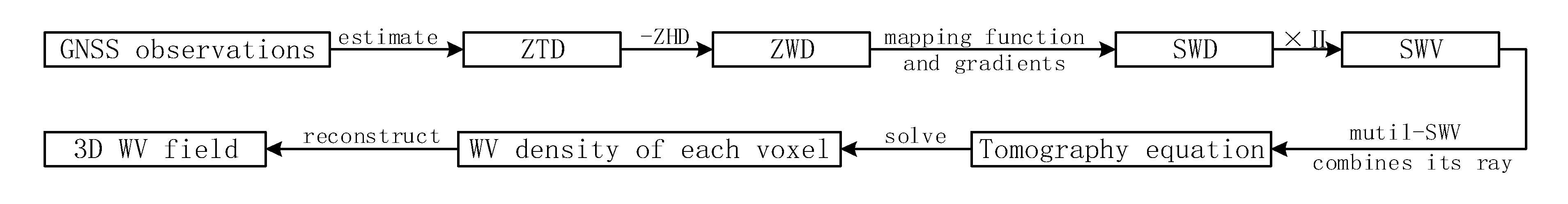
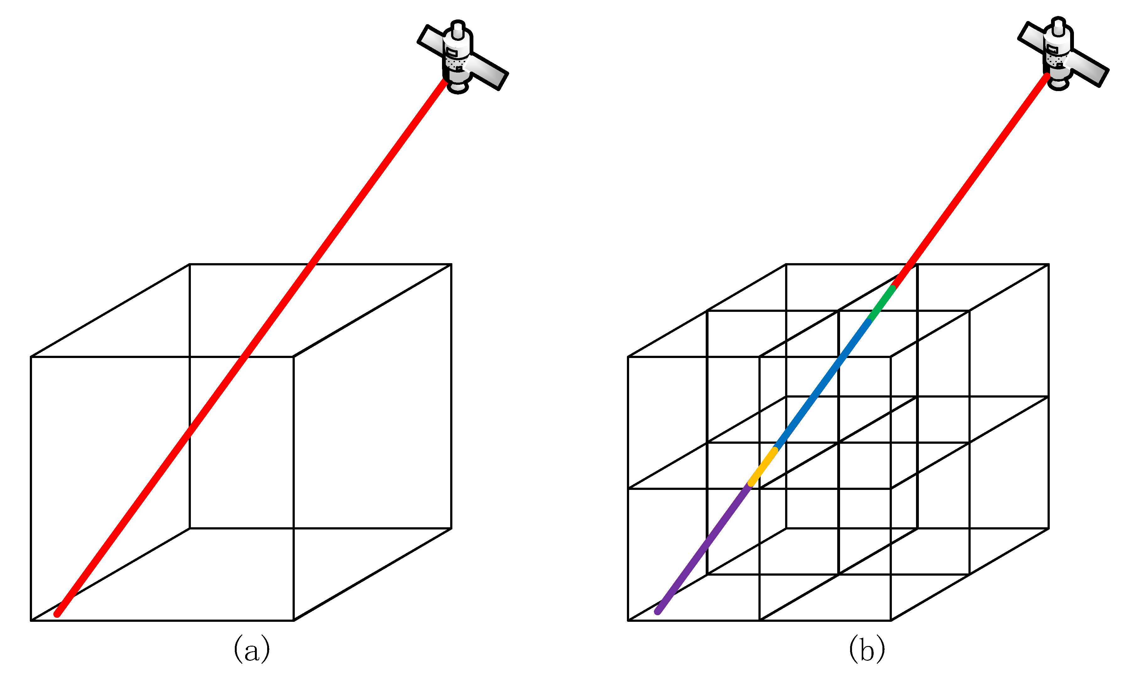
As shown in Figure 1, we can reconstruct the WV field with GNSS tropospheric tomography by the following processes. The zenith wet delay (ZWD) can be obtained from the ZTD retrieved from GNSS observations by subtracting the zenith hydrostatic delay (ZHD) computed by the Saastamoinen model [21]. The slant wet delay (SWD) is usually restored from the ZWD using the mapping function and gradient, and then multiplying by the conversion parameter, which yields the slant wet vapor (SWV). The SWV is the key parameter for the resulting 3D WV retrieval. Next, we have to divide the tomography zone into a finite number of voxels. These voxels discretized the valid rays (as shown in Figure 2a, refer to the rays passing from the top boundary of the tomography zone to the receivers) into several segments (Figure 2b). Combing their corresponding SWV, all valid rays are assembled into the tomography equations. Solving the above tomography equations, we can obtain the WV density of each voxel. Based on these voxels with WV values, the 3D WV field can finally be reconstructed. The details of these processes will be present in the following sections.
The equations involved above are as follows:
where is the SWV of a valid signal . refers to the intercept of the signal in the voxel , whereas is the WV density of the above voxel. Valid signals determine Equation (4), which are converted to Equation (5) for convenience.
After solving Equation (5), we can obtain the WV content of ray-passed voxels. Based on these voxels with their WV values, a completed 3D WV field over a study area can finally be reconstructed. Investigations have proven that the iterative algorithm has good performance in solving the tomography equations (Equation (5)). Hence, we adopted a commonly used Kalman filtering (KF) technique [22,23] for the tomography solution.
2.2. General Tomographic Window and Existing Problems
The tomographic window has reached widespread applications in previous studies [24,25,26]. This “window” is based on the assumption that the WV of interest remains stationary across a period, and the length of the period determines the size of the window. In general, the tomographic window is set to cover signals from selected epochs of a continuous period. The quantity of selected epochs demonstrates the multiple signal increases.
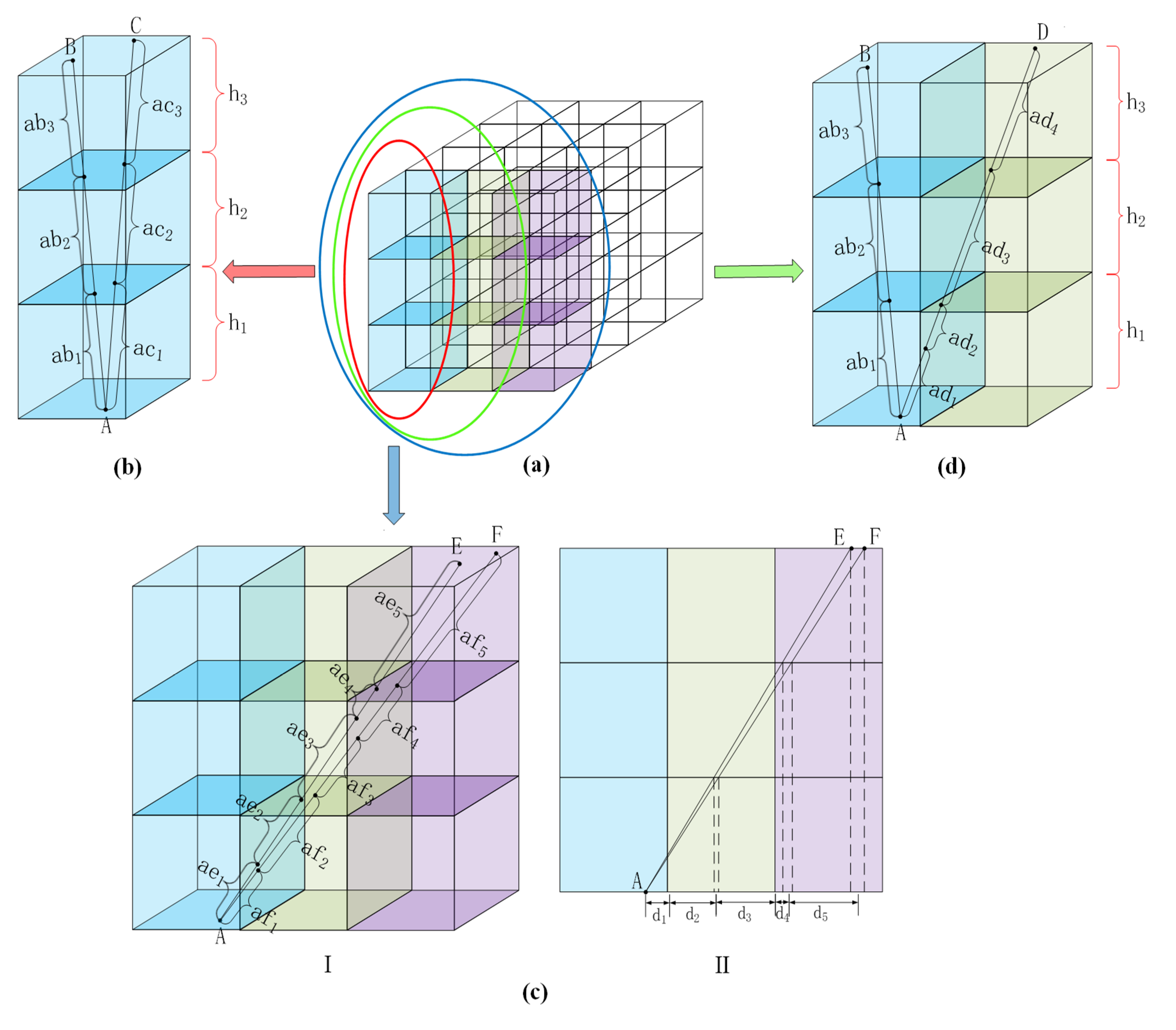
In theory, using the tomography window can multiply the number of valid signals to significantly increase the rank of the tomography coefficient matrix. However, the effect of this approach is not ideal in practice. The increase in rank score was not as expected. Here, we introduce the concept of characteristic signals to explain the underlying reasons for the above phenomenon. All characteristic signals belong to valid signals, but only nonlinear dependent parts can be considered as characteristic signals. We show the difference between valid and characteristic signals in Figure 3. Figure 3a shows a tomographic region discretizing into several voxels and part of them are circled for signal visualization. Two of the visualized rays (A–B) and (A–C) are shown in Figure 3b. Both of the rays mentioned above are valid signals and are divided into three-line segments by voxels. A linear dependence exists in the segments. The dependence can be described as follows:
Equation (6) reveals that massive valid signals concentrated around the zenith (most of them only passing through voxels in the same column), because of their strong dependence, provide less useful information to the tomography equation. These valid signals result in a linear dependence in the tomography equation that subsequently renders its rank score far less than the number of valid signals.
Similarly, Figure 3c I shows another case of linear dependence that occurred in the valid signals. Ray (A–E) and (A–F) cross through the same voxels, and their segments divided by the above voxels exhibit a similar proportion (Figure 3c II). The proportional relationship between the two sets of segments originated from the line (A–E)/(A–F) and can be expressed as:
Some valid signals show the relationship in the above equation, and such signals will be eliminated after the elementary row transformation.
Moreover, Figure 3d presents another type of valid signal that passes through different columns of voxels. The line (A–D) is divided into four segments by voxels but the line (A–C) is divided into three parts; evidently, there is no linear dependence between the two lines. This type of signal represents an independent equation, which forms a stable system of tomography equations with a rank score equal to the number of rays, which can effectively express the information of the WV distribution. We define these signals as the characteristic signals.
Overall, because a large number of valid signals exhibit a dependent relationship, as shown in Equations (6) and (7), even with the introduction of massive valid signals, the tomography equation will yield minor rank score improvement. However, the massive signals will bring a high condition number to the tomography equation itself, which causes a severe ill-condition problem. Therefore, owing to low coverage of characteristic signals, the purposeless selection of epochs (general tomographic window) has limited gain to the tomography equation.
2.3. Refined Tomographic Window
A reasonable tomographic window should consider all possible characteristic signals. A feasible setting for the tomographic window is to cover all signals of settled duration (i.e., signals of all epochs in the selected period). Undoubtedly, this setting does not ignore any characteristic signals; however, it may seriously increase the amount of calculation and results in a significant ill-condition problem. Thus, it is not an appropriate solution to the tomographic window. Herein, we propose an alternative tomographic window, which covers all characteristic signals but is also timesaving as compared to the former. The proposed tomographic window automatically retains only the characteristic signals traversing the signals of all epochs in the selected period.
The objective of the process of “traversals” is to reasonably separate the characteristic signals from the multitude of valid signals. The kernel of the above processes is classified and filtered toward the signals. Firstly, we classified the valid signals into the following types: (1) rays from the same receiver and only crossing one column of voxels (red rays in Figure 4); (2) rays similar to (1) but from different receivers, which are located in the same bottom voxels with ray 1 (red and green rays in Figure 4); (3) rays from the same receiver and crossing the same voxels located in different columns (blue rays in Figure 4). Notability, few rays come from different receivers but pass through the same voxels in different columns, such that we ignore the rays belonging to this type.
Then, we can eliminate the redundant parts of valid signals in two steps:
Step 1: As shown in Figure 4, for valid signals belonging to case 1, we first compared the SWV they carry. If these SWVs show a similar value (the range is less than 10 mm), the proposed tomographic window directly reserves a single ray (solid in red and green), as well as eliminates the rest (red and green dashed lines). If not, the tomographic window repeats the above process but the SWV value of the ray reserved was adjusted to the average value of the SWVs carried by case 1 rays.
Step 2: Completed step 1, each site in Figure 4 remains a single ray that only crosses the column voxels where the site is located. If these rays follow case 2, the SWV corresponding to them is approximately equal (the range is less than 10 mm), we keep one of these rays. If the range of the SWVs is greater than 10 mm, we retain these rays.
Step 3: If the rays follow case 3 and have similar SWV, we only keep one of them. However, we execute operations similar to those in the previous two steps if the SWVs belonging to the rays exhibit a large difference.
Based on the above three steps, the refined tomographic window can accomplish the screening of characteristic signals or the elimination of redundant rays.
3. GNSS Network and Data Preprocessing
3.1. Hong Kong CORS
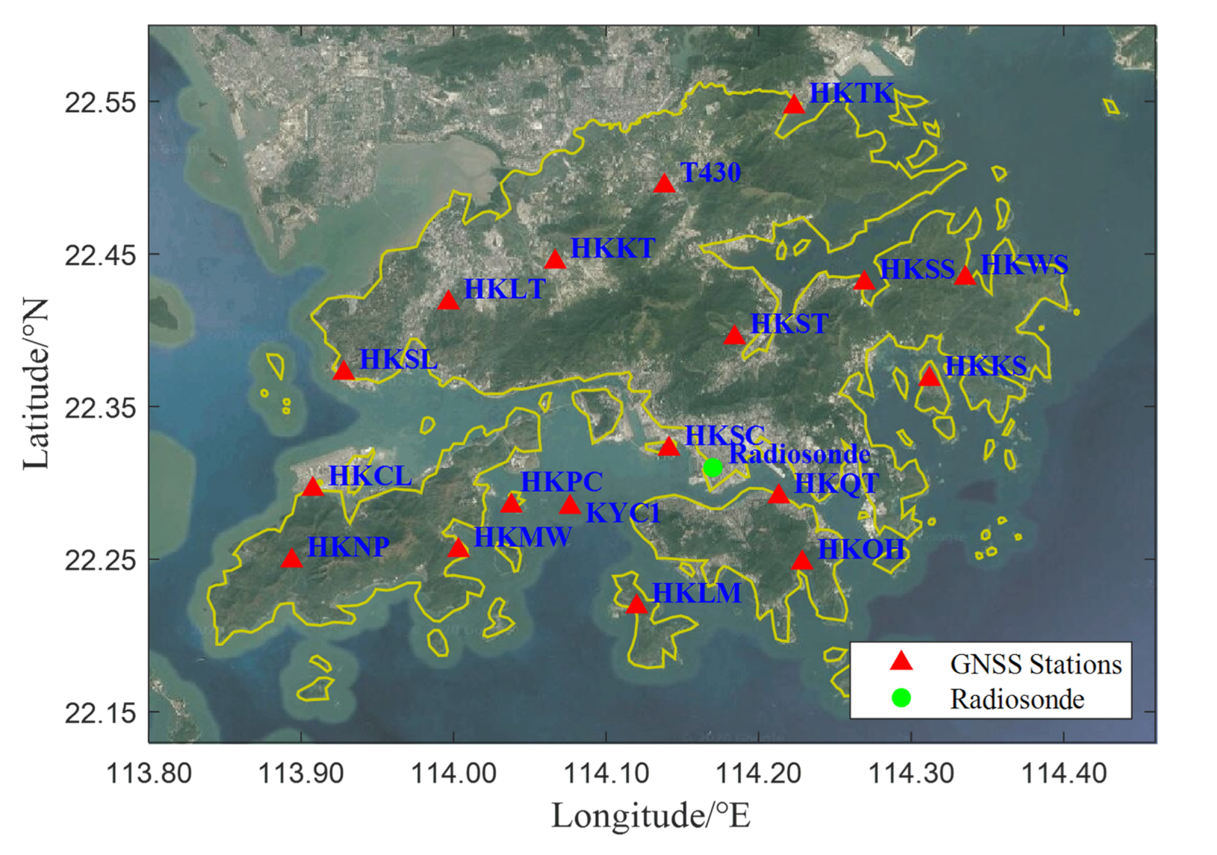
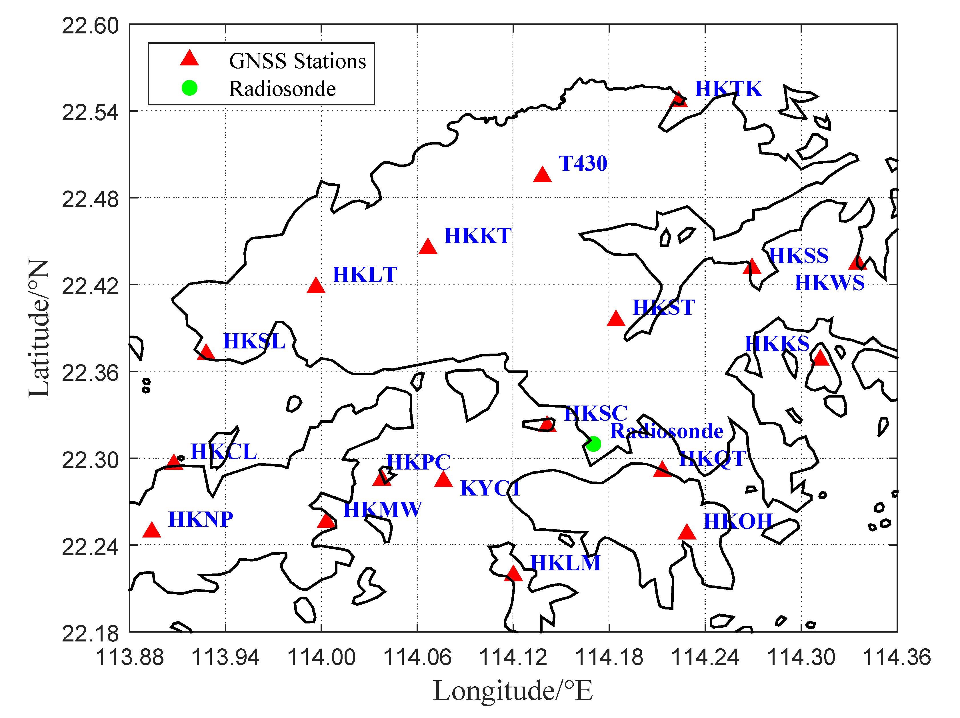
The Hong Kong (HK) CORS satellite positioning reference station network (SatRef) consists of 18 permanent GNSS observations (red triangles in Figure 5). Most stations are equipped with an automatic meteorological sensor that records temperature, pressure, and relative humidity. With these data, the tropospheric ZHD can be accurately separated by the Saastamoinen model. This is one advantage of SatRef for GNSS-derived WV tomography. The other is that the mean geographic distance between stations is approximately 10 km and contributes massive SWV to a tomography grid. Furthermore, a RS station (green circle in Figure 5) is located in the HK area that can provide accurate 3D WV distribution, which has valuable information as an initial value and reference for GNSS-WV tomography.
3.2. Grid Scheme
According to a previous study [27], the optimized voxel scheme was applied in GNSS-WV tomography. The optimized voxels refer to ray-passed through voxels, i.e., in the tomography processes, only ray-passed through voxels participate to establish the tomography equation. Furthermore, the optimized voxel scheme supports a constraint-free strategy, which can prevent the tomography results from the interference of constraints that originated from empirical functions. Because of the aforementioned advantage, this investigation in the HK area adopted the optimized voxels.
Based on the existing research [15,24], we determined the horizontal grid scheme shown in Figure 6. The figure shows that the selected horizontal domain with a scope of 22.18°–22.60°N, 113.88°–114.36°E, was discretized into 7 × 8 grids, 7 in the latitudinal and 8 in the longitudinal direction. This means the horizontal resolutions of the study are both 0.06°in latitude and longitude. Regarding the vertical strategy, we divided the troposphere over HK into 12 layers with a thickness of 0.5, 0.5, 0.7, 0.7, 0.7, 0.9, 0.9, 0.9, 1.1, 1.1, 1.1, and 1.1 km (Figure 7). Overall, the study area (tomography zone) was discretized into 7 × 8 × 12 voxels.
3.3. Data Preprocessing
To evaluate the performance of the GNSS-WV tomography technique, we collected observations of SatRef in two periods. One is from 10 May to 12 May when the weather was clear. The other was from 26 May to 28 May when the HK area suffered heavy rain. The 6 d of observation above were derived from 18 stations and were processed by the double-differenced module using GAMIT software (version: 10.71) [28]. Notably, tropospheric parameters exhibit a strong correlation in a small area, which means the SWV cannot be estimated correctly in a dense GNSS network (SatRef, in this case). To weaken this correlation, we selected four additional International GNSS Service (IGS) stations (BJFS, SHAO, WUHN, and JFNG) to incorporate the baseline solution. Additionally, we estimated ZTD and gradients with the intervals of 0.5 h by using the above GAMIT software. Subtracting the ZHD computed by the Saastamoinen model, we could obtain ZWD. Then, based on the aforementioned gradients, SWD could be obtained by projecting the ZWD onto the slant path. Combing conversion parameter II, we finally retrieved the SWV that was a prerequisite to establishing the tomography equation (recall Figure 1).
4. Experiment and Results
To evaluate the performance of the proposed tomography method, we designed the comparative experiments between the traditional method and improved approach, identified as Methods 1 and 2, respectively. We firstly present the experimental description (including the selected test period and the accuracy indicator used), and the experimental results are then presented.
4.1. Experiment Description
To verify the performance and applicability of the above tomography approaches, we collected the GNSS observations of SatRef (Figure 5) in two periods under different weather conditions (Table 1). The first was from 10 May to 12 May 2019 (day of year (DOY) 130 to 132) when the weather was clear or cloudy; the other was from 26 May to 28 May 2019 (DOY 146 to 148), whereas HK suffered heavy rain. We adopted the grid scheme described in Section 3.2 to discretize the tomography area into finite independent voxels. Completing the discrete process, each valid signal with its SWV was retrieved based on the data preprocessing presented in Section 3.3. As RS launched at UTC 00:00 and 12:00 daily, we could obtain two-epoch accurate WV profiles per day for tomographic method comparison. Thus, we accordingly collected the appropriate valid rays at the above test epochs for the tomography experiment. Based on these rays, using the general and refined tomographic window (Section 2.2 and Section 2.3), we assembled the conventional tomography equation (used in Method 1) and improved tomography equation (applied by Method 2), respectively. The aforementioned equations were then solved by the KF method (Section 2.1).
Moreover, the root mean square error (RMSE), mean absolute error (MAE), and bias were used as accuracy indicators to quantify the deviation of tomography results against the truth (RS-Method).
4.2. Tomography Results for The Comparison Between Methods 1 and 2
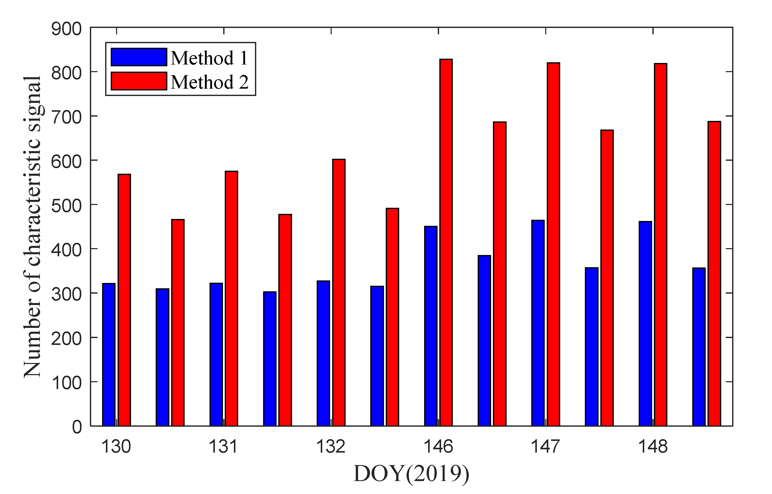
The statistics for the quantity of the characteristic signal used in Methods 1 and 2 at the test epochs are shown in Figure 8. It revealed that using refined tomographic windows, Method 2 imposed much more (approximate 75.9%) characteristic signals than did Method 1 into the tomography equation at all test periods. Notability, in the second period (DOY 146–148, 2019), each station in SatRef was operating but one site did not work during the first period (DOY 130–132, 2019). This led to more GNSS observations in period 2, which explains why SatRef during period 2 provided a relatively larger quantity of characteristic signals than in period 1.
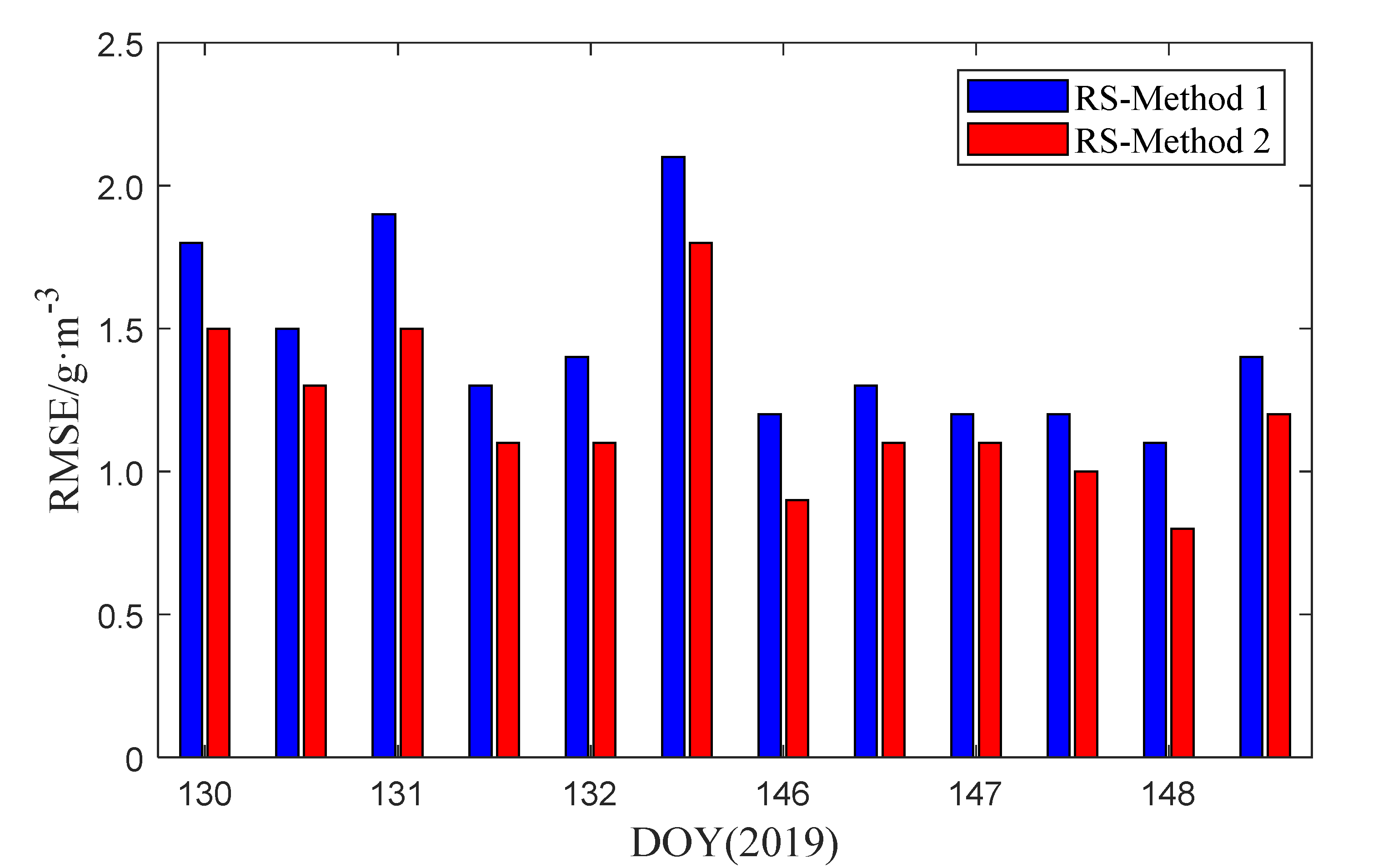
Regarding whether considering more characteristic signals are beneficial to acquiring more accurate 3D WV products, we needed to compare the tomographic results of the two methods. We first interpolated WV density profiles obtained by RS to the tomography voxel center. Furthermore, the WV profiles for the location of the RS were calculated using the GNSS-WV tomography technique based on the two methods during the experimental epochs, respectively. Then, the RMSE of RS-Method 1 (blue bar) and RS-Method 2 (red bar) were computed for each epoch over the test period and are shown in Figure 9. For the RS comparison (assumed as the truth), the RMSEs of Method 2 were less than those of Method 1 in all test epochs. This indicated that Method 2 exhibited better WV estimation accuracy than Method 1, which showed that more characteristic signals included in the tomography equation could effectively increase the performance of the GNSS-WV tomography technique. Additionally, both of the methods showed a relatively smaller RMSE during rainy weather (DOY 146–148, 2019) than during rainless weather (DOY 130–132, 2019).
For an intuitive comparison, the RMSE statistics of the two tomography methods during the rainy period and rainless period are listed in Table 2. It can be seen that for the RS data comparison, RMSE of Method 1 was 1.7 g/m3 on clear days, but decreased to 1.2 g/m3 on rainy days. A similar result occurred in Method 2 wherein RMSE decreased from 1.4 (rainless days) to 1.0 g/m3 (rainy days). This revealed that the GNSS-WV tomography exhibited better performance during rainy days than the rainless day. Furthermore, in the case of rainless days, the RMSE of the WV profile derived from the proposed and conventional methods were 1.4 and 1.7 g/m3, respectively, which indicated that by using more characteristic signals, the accuracy of the tomography method was increased by 17.6%. Similarly, in rainy weather, the performance of the method proposed improved by 16.7%.
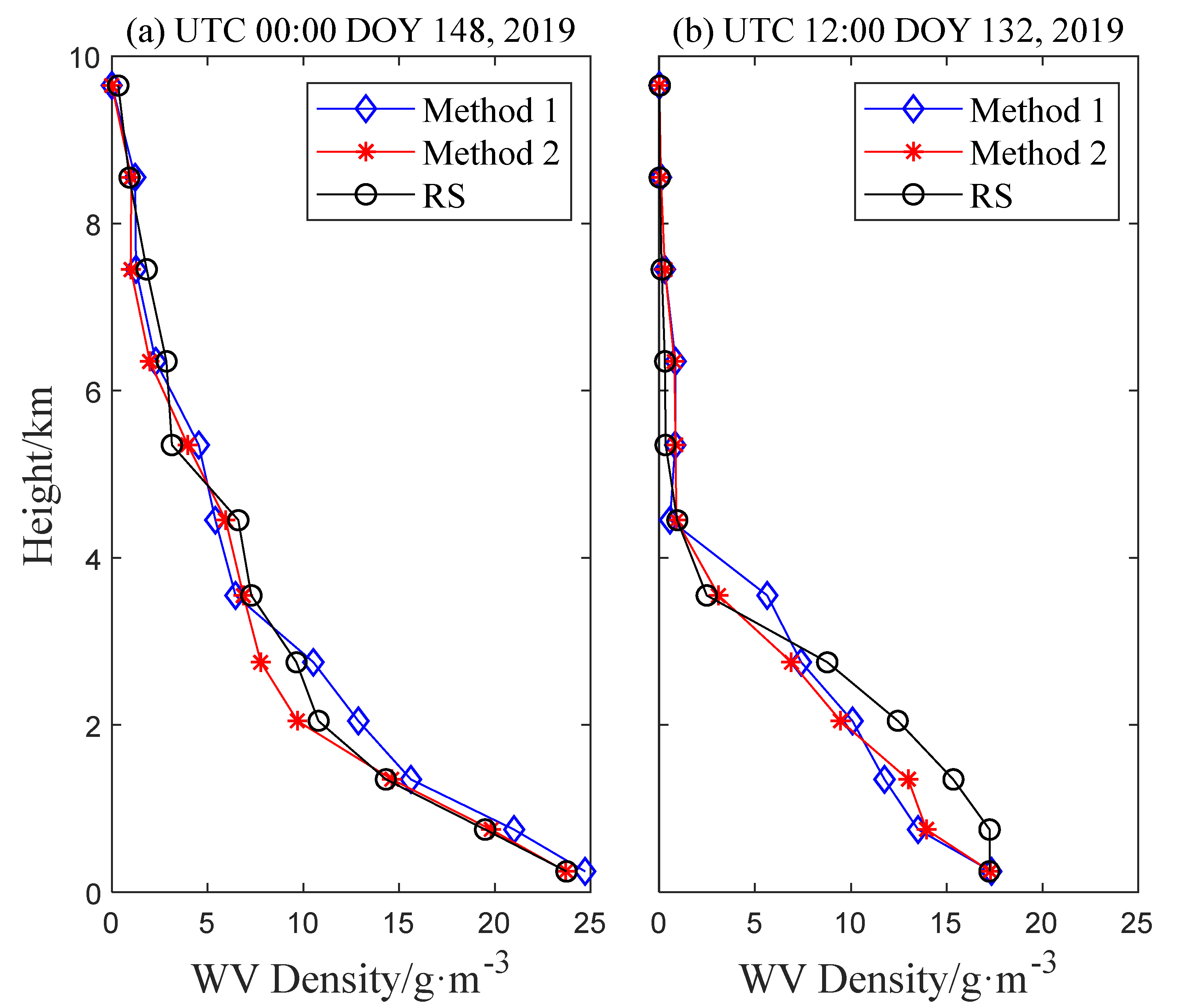
To understand why the GNSS-WV tomography exhibited higher performance during the rainy period, we selected the two epochs with the minimum and maximum RMSEs for both Methods 1 and 2. The comparison of the WV profiles derived from two tomography methods and RS-Method during the above two epochs are shown in Figure 10. As shown in Figure 10a, at UTC 00:00 DOY 148, 2019 (rainy), the WV profiles derived from Methods 1 and 2 matched the RS-WV profile well. Figure 10b shows that at UTC 12:00 DOY 132, 2019 (rainless), a relatively large difference in WV profiles was generated from the two tomography methods and the RS data. A clear difference between Figure 10a,b is in the vertical distribution of WV. The RS-WV shown in Figure 10a is more even than that in Figure 10b, which is near the ideal WV distribution in the vertical direction. Zhang et al. [24] stated that the WV with an even distribution is beneficial for good tomography results obtained by the GNSS-WV tomography. Hence, at the epoch in Figure 10a, the WV profiles obtained by the two tomography methods were in good agreement with that obtained by the RS-Method. However, on a clear day, RS-WV exhibited a large value below 4 km, but smaller value over 4 km, it indicated that the WV was more concentrated near the ground during this period than during rainy days. This sudden change occurred in the content of WV and led to an inaccurate perception of the two tomography methods. Overall, the actual distribution of WV affected the performance of the GNSS-WV tomography technique: the more even the vertical distribution of WV, the better the results of GNSS-WV tomography, and vice versa.
To verify the improvement of the proposed tomography methods in general, the bias, MAE, and RMSE between the RS and the two methods for the test period are analyzed and listed in Table 3. The statistical results showed that the bias/MAE/RMSE of RS-Method 2 were smaller than that of Method 1, with the value of −0.1/0.9/1.2 and −0.2/1.1/1.5 g/m3, respectively. It can be seen that Method 2 significantly outperformed Scheme 1 in all three accuracy indicators in Table 3, which indicated again that, by using a refined tomographic window, Method 2 obtained a superior tomography result compared with that of Method 1 (based on a general tomographic window). Additionally, negative bias demonstrated that the GNSS-WV tomography has the problem of overestimating the WV content of the troposphere. Moreover, compared to Method 1, the RMSE of the method decreased 0.3 g/m3 from 1.5 to 1.2 g/m3, which revealed the accuracy of the proposed tomography method (Method 2) was improved by 20.0% over the conventional method (Method 1).
Furthermore, the RMSE and relative error [29] of the two tomography methods at each layer for the experimental period were calculated and are shown in Figure 11. We found that variation in RMSE and relative error for both methods exhibited a similar trend with altitude. RMSE of the two tomography methods decreased with the increase of altitude in general, but the relative error showed the opposite trend. Notably, the RMSE of RS-Methods 1 and 2 presented a large value below 4 km (Figure 11a). The lower troposphere is one of the most active parts of the whole, where a great deal of variable WV concentrates. Therefore, these abundant and varied WV values present a challenge in retrieving its 3D distribution in GNSS-WV tomography. A similar phenomenon in Figure 11b is that the relative error of both methods at the corresponding height range showed sharp growth. This revealed a drawback in GNSS-WV tomography. It cannot accurately sense WV content in the lower troposphere. However, in the lower layers (below 4 km), the improved method (red line) still showed a smaller RMSE and relative error than the conventional method (blue line). This result also validated the superiority of the improved tomography method. Additionally, it should be noted that the relative error of the two methods was approximate to 100% above 8 km (Figure 11b). This phenomenon is not evident in the poor performance of GNSS-WV tomography in the higher layers of the troposphere. The reason for this result lies in low WV content in the upper layers, and even a small diversion could cause a large relative error.
5. Discussion
In the above tomography experiments, the proposed tomography method (Method 2), using a refined tomographic window, introduced more characteristic signals into the tomography model as well as eliminated redundant signals and consequently gets better 3D WV density than the traditional method (Method 1). The results indicate that more characteristic signals and less redundant signals are benefits to GNSS-WV tomography algorithm for a better WV estimation. To ensure the reliability of the experimental results, the variance test was conducted. The WV density results from Methods 1 and 2 do not follow the normal distribution; therefore, we select commonly used non-parametric inferential statistical method: Friedman tests [30]. The null hypothesis is that there is no significant difference between the tomography results obtained by the aforementioned methods. Table 4 listed the result of the Friedman test toward the WV data belongs to Methods 1 and 2 in detail. The F statistic and P statistic are 4.123 and 0.045, respectively. Meanwhile, according to the F-distribution table for , we found that . Since the F statistic (4.123) is greater than the F critical value (3.842) and P statistic is less than 0.05, we accept the alternative hypothesis and conclude that there is a statistically significant difference between the two different tomography methods with a 95% level of confidence.
6. Conclusions
We proposed an improved GNSS-derived water vapor (WV) tomography method based on a refined tomographic window. The kernel of the refined window separates the characteristic signal (nonlinear correlated signals) from massive valid signals. A conventional tomography method using a general tomographic window was adopted as a comparison. Comparative experiments were conducted in the Hong Kong (HK) area during two selected periods under rainy and rainless weather conditions. Statistics of the characteristic signals demonstrated that the improved method introduced 75.9% more characteristic signals than the conventional method into the tomography equation. WV profiles reconstructed by the above tomography methods were then validated by radiosonde (RS) data. Test results showed that, compared to the conventional method, the improved method could retrieve relatively accurate WV information under different weather conditions. Therefore, using a refined tomographic window, the improved method can consider more characteristic signals and eliminate redundant valid signals, which significantly optimized the tomography coefficient matrix (i.e., increased its rank score and simultaneously reduced its condition numbers). In consequence, the improved method obtained superior tomography results. It is expected that the more characteristic signals, the more accurate the three-dimensional WV information derived by GNSS-WV tomography. Hence, further studies should be conducted to consider more GNSS observations from operational multi-GNSS systems (GPS, BDS, GLONASS, and GALILEO) for a larger quantity of characteristic signals.
Author Contributions
Conceptualization, Y.Y. and C.L.; methodology, Y.Y. and C.L.; validation, Y.Y. and C.X.; data curation, C.L., Y.T. and M.F.; funding acquisition, Y.Y., Y.T. and M.F.; writing—original draft preparation, Y.Y. and C.L.; writing—review and editing, Y.Y., C.L. and C.X. All authors have read and agreed to the published version of the manuscript.
Funding
This research was funded by the National Natural Science Foundation of China, grant number 41721003. Besides, this work was supported by 2019 Key Technology Projects of Transportation Industry, grant number 2019-MS1-013, and Science and Technology Project of Highway Construction Engineering of Zhejiang Provincial Department of Transportation, grant number 2019-GCKY-02.
Acknowledgments
The authors would like to thank the International GNSS Service (IGS), the Lands Department of HKSAR, and the Hong Kong Observatory (HKO) for the provision of data and products. The authors are grateful to anonymous reviewers.
Conflicts of Interest
The authors declare no conflict of interest.
References
- Bevis, M.; Businger, S.; Herring, T.A.; Rocken, C.; Anthes, R.A.; Ware, R.H. GPS meteorology: Remote sensing of atmospheric water vapor using the Global Positioning System. J. Geophys. Res. Atmos. 1992, 97, 15787–15801. [Google Scholar] [CrossRef]
- Rocken, C.; Ware, R.; van Hove, T.; Solheim, F.; Alber, C.; Johnson, J.; Bevis, M.; Businger, S. Sensing atmospheric water vapor with the Global Positioning System. Geophys. Res. Lett. 1993, 20, 2631–2634. [Google Scholar] [CrossRef] [Green Version]
- Zhao, Q.; Liu, Y.; Ma, X.; Yao, W.; Yao, Y.; Li, X. An improved rainfall forecasting model based on GNSS observations. IEEE Trans. Geosci. Remote Sens. 2020, 58, 4891–4900. [Google Scholar] [CrossRef]
- Zhao, Q.; Ma, X.; Yao, Y. Preliminary result of capturing the signature of heavy rainfall events using the 2-d-/4-d water vapour information derived from GNSS measurement in Hong Kong. Adv. Space Res. 2020, 66, 1537–1550. [Google Scholar] [CrossRef]
- Zhao, Q.; Liu, Y.; Yao, W.; Ma, X.; Yao, Y. A novel ENSO monitoring method using precipitable water vapor and temperature in southeast China. Remote Sens. 2020, 12, 649. [Google Scholar] [CrossRef] [Green Version]
- Zhao, Q.; Ma, X.; Yao, W.; Yao, Y. A new typhoon-monitoring method using precipitation water vapor. Remote Sens. 2019, 11, 2845. [Google Scholar] [CrossRef] [Green Version]
- Chen, B.; Liu, Z. Voxel-optimized regional water vapor tomography and comparison with radiosonde and numerical weather model. J. Geodesy. 2014, 88, 691–703. [Google Scholar] [CrossRef]
- Li, X.; Zus, F.; Lu, C.; Ning, T.; Dick, G.; Ge, M.; Wickert, J.; Schuh, H. Retrieving high-resolution tropospheric gradients from multiconstellation GNSS observations. Geophys. Res. Lett. 2015, 42, 4173–4181. [Google Scholar] [CrossRef] [Green Version]
- Alshawaf, F.; Fuhrmann, T.; Knöpfler, A.; Luo, X.; Mayer, M.; Hinz, S.; Heck, B. Accurate estimation of atmospheric water vapor using GNSS observations and surface meteorological data. IEEE Trans. Geosci. Remote Sens. 2015, 53, 3764–3771. [Google Scholar] [CrossRef]
- Yao, Y.; Shan, L.; Zhao, Q. Establishing a method of short-term rainfall forecasting based on GNSS-derived PWV and its application. Sci. Rep. 2017, 7, 1–11. [Google Scholar] [CrossRef]
- Liu, C.; Zheng, N.; Zhang, K.; Liu, J. A new method for refining the GNSS-derived precipitable water vapor map. Sensors 2019, 19, 698. [Google Scholar] [CrossRef] [Green Version]
- Zhang, B.; Fan, Q.; Yao, Y.; Xu, C.; Li, X. An improved tomography approach based on adaptive smoothing and ground meteorological observations. Remote Sens. 2017, 9, 886. [Google Scholar] [CrossRef] [Green Version]
- Flores, A.; Ruffini, G.; Rius, A. 4D tropospheric tomography using GPS slant wet delays. Ann. Geophys. 2000, 18, 223–234. [Google Scholar] [CrossRef]
- Zhao, Q.; Zhang, K.; Yao, Y.; Li, X. A new troposphere tomography algorithm with a truncation factor model (TFM) for GNSS networks. GPS Solut. 2019, 23, 64. [Google Scholar] [CrossRef]
- Zhao, Q.; Yao, W.; Yao, Y.; Li, X. An improved GNSS tropospheric tomography method with the GPT2w model. GPS Solut. 2020, 24, 1–13. [Google Scholar] [CrossRef]
- Rohm, W.; Bosy, J. The verification of GNSS tropospheric tomography model in a mountainous area. Adv. Space Res. 2011, 47, 1721–1730. [Google Scholar] [CrossRef]
- Alshawaf, F. Constructing Water Vapor Maps by Fusing InSAR, GNSS, and WRF Data. Ph.D. Thesis, Karlsruhe Institute of Technology, Karlsruhe, Germany, 2013. [Google Scholar]
- Benevides, P.; Catalao, J.; Nico, G.; Miranda, P.M. Inclusion of high resolution MODIS maps on a 3D tropospheric water vapor GPS tomography model. In Proceedings of the Remote Sensing of Clouds and the Atmosphere XX, Toulouse, France, 16 October 2015; p. 96400R. [Google Scholar]
- Ye, S.; Xia, P.; Cai, C. Optimization of GPS water vapor tomography technique with radiosonde and COSMIC historical data. Ann. Geophys. 2016, 34, 789–799. [Google Scholar] [CrossRef] [Green Version]
- Chen, B.; Liu, Z. Assessing the performance of troposphere tomographic modeling using multi-source water vapor data during Hong Kong’s rainy season from May to October 2013. Atmos. Meas. Tech. 2016, 9, 5249–5263. [Google Scholar] [CrossRef] [Green Version]
- Saastamoinen, J. Atmospheric correction for the troposphere and stratosphere in radio ranging satellites. Bull. Géodésique 1972, 15, 247–251. [Google Scholar]
- Nilsson, T.; Gradinarsky, L. Water vapor tomography using GPS phase observations: Simulation results. IEEE Trans. Geosci. Remote Sens. 2006, 44, 2927–2941. [Google Scholar] [CrossRef]
- Ding, W.; Wang, J.; Rizos, C.; Kinlyside, D. Improving adaptive Kalman estimation in GPS/INS integration. J. Navig. 2007, 60, 517–529. [Google Scholar] [CrossRef] [Green Version]
- Zhao, Q.; Yao, Y.; Cao, X.; Zhou, F.; Xia, P. An optimal tropospheric tomography method based on the multi-GNSS observations. Remote Sens. 2018, 10, 234. [Google Scholar] [CrossRef] [Green Version]
- Dong, Z.; Jin, S. 3-D water vapor tomography in Wuhan from GPS, BDS and GLONASS observations. Remote Sens. 2018, 10, 62. [Google Scholar] [CrossRef] [Green Version]
- Troller, M.R. GPS Based Determination of the Integrated and Spatially Distributed Water Vapor in the Troposphere. Ph.D. Thesis, ETH Zurich, Zürich, Switzerland, 2004. [Google Scholar]
- Yao, Y.; Liu, C.; Xu, C. A new GNSS-Derived water vapor tomography method based on optimized voxel for large GNSS network. Remote Sens. 2020, 12, 2306. [Google Scholar] [CrossRef]
- Herring, T.; King, R.; Floyd, M.; McClusky, S. GAMIT Reference Manual, GPS Analysis at MIT; Department of Earth, Atmospheric, and Planetary Sciences, Massachussets Institute of Technology: Cambridge, MA, USA, 2018. [Google Scholar]
- Zhang, W.; Zhang, S.; Nan, D.; Pengxu, M. An improved tropospheric tomography method based on the dynamic node parametrized algorithm. Acta Geodyn. Geomater. 2020, 17, 191–206. [Google Scholar] [CrossRef]
- Friedman, M. The use of ranks to avoid the assumption of normality implicit in the analysis of variance. J. Am. Stat. Assoc. 1937, 32, 675–701. [Google Scholar] [CrossRef]
Figure 1.
Process of reconstruction of the three-dimensional (3D) water vapor (WV) information using the global navigation satellite system (GNSS) tomography technique.
Figure 1.
Process of reconstruction of the three-dimensional (3D) water vapor (WV) information using the global navigation satellite system (GNSS) tomography technique.

Figure 2.
Valid ray: (a) valid ray penetrating from the top boundary of the tomography area and reaching the receivers; (b) valid ray discretized by voxels.
Figure 2.
Valid ray: (a) valid ray penetrating from the top boundary of the tomography area and reaching the receivers; (b) valid ray discretized by voxels.

Figure 3.
Difference between valid and characteristic signals: (a) a tomography area composed of voxels, with one column of voxels circled in red, whereas two columns of voxels are circled in green and three columns of voxels are in purple circle; (b) visualization of valid signals (A–B) and (A–C); (c) visualization of valid signals (A–E) and (A–F); (d) visualization of characteristic signals (A–B) and (A–D).

Figure 4.
Redundancy of two types of valid signals.

Figure 5.
Geographic distribution of 18 GNSS stations (red triangles) and 1 radiosonde (RS) station (green circle) in Hong Kong (HK).
Figure 5.
Geographic distribution of 18 GNSS stations (red triangles) and 1 radiosonde (RS) station (green circle) in Hong Kong (HK).

Figure 6.
Horizontal grid scheme in the study area. The selected study area was divided into a 7 × 8 grid, 7 in the latitudinal and 8 in the longitudinal direction.
Figure 6.
Horizontal grid scheme in the study area. The selected study area was divided into a 7 × 8 grid, 7 in the latitudinal and 8 in the longitudinal direction.

Figure 7.
Vertical grid strategy in the study area. The troposphere over HK was divided into 12 layers from bottom to top with thicknesses of 0.5, 0.5, 0.7, 0.7, 0.7, 0.9, 0.9, 0.9, 1.1, 1.1 1.1, and 1.1 km.
Figure 7.
Vertical grid strategy in the study area. The troposphere over HK was divided into 12 layers from bottom to top with thicknesses of 0.5, 0.5, 0.7, 0.7, 0.7, 0.9, 0.9, 0.9, 1.1, 1.1 1.1, and 1.1 km.

Figure 8.
Number of characteristic signals used for different tomography methods at UTC 00:00 and 12:00 during the experimental period from DOY 130–132, 2019, and DOY 146–148, 2019.
Figure 8.
Number of characteristic signals used for different tomography methods at UTC 00:00 and 12:00 during the experimental period from DOY 130–132, 2019, and DOY 146–148, 2019.

Figure 9.
Root mean square error (RMSE) comparison between RS and the two tomography methods for the period of DOY 130–132, 146–148, 2019.
Figure 9.
Root mean square error (RMSE) comparison between RS and the two tomography methods for the period of DOY 130–132, 146–148, 2019.

Figure 10.
WV profiles comparisons derived from different tomography methods and RS at UTC 00:00 DOY 148, 2019 (a), and UTC 12:00 DOY 132, 2019 (b). Additionally, the RMSE of both tomography methods was least in epoch (a) but most in epoch (b).
Figure 10.
WV profiles comparisons derived from different tomography methods and RS at UTC 00:00 DOY 148, 2019 (a), and UTC 12:00 DOY 132, 2019 (b). Additionally, the RMSE of both tomography methods was least in epoch (a) but most in epoch (b).

Figure 11.
RMSE (a) and relative error (b) at different altitudes of the tomography results from Methods 1 and 2 with respect to the RS-Method.
Figure 11.
RMSE (a) and relative error (b) at different altitudes of the tomography results from Methods 1 and 2 with respect to the RS-Method.


Table 1.
Selected periods with their weather conditions.
| Period | Day-of-Year (DOY) | Weather Conditions |
|---|---|---|
| 1 | 130–132 | rainless |
| 2 | 146–148 | rainy |
Table 2.
Statistical results of tomography accuracy considering the radiosonde (RS) method as the reference under different weather conditions (g/m3).
Table 2.
Statistical results of tomography accuracy considering the radiosonde (RS) method as the reference under different weather conditions (g/m3).
| Root Mean Square Error (RMSE) (Rainless) | RMSE (Rainy) | |
|---|---|---|
| RS-Method 1 | 1.7 | 1.2 |
| RS-Method 2 | 1.4 | 1.0 |
Table 3.
Statistical comparison of RS-Methods 1 and 2 in the experimental period (g/m3).
| Bias | Mean Absolute Error (MAE) | RMSE | |
|---|---|---|---|
| RS-Method 1 | −0.2 | 1.1 | 1.5 |
| RS-Method 2 | −0.1 | 0.9 | 1.2 |
Table 4.
Friedman’s analysis of variance (ANOVA) table for the experimental results of Methods 1 and 2.
Table 4.
Friedman’s analysis of variance (ANOVA) table for the experimental results of Methods 1 and 2.
| Source | Sum of Squares (SS) | Degrees of Freedom (df) | Mean Squares (MS) | F | P |
|---|---|---|---|---|---|
| Columns | 1.806 | 1 | 1.806 | 4.123 | 0.045 |
| Error | 58.194 | 143 | 0.438 | ||
| Total | 60 | 287 |
© 2020 by the authors. Licensee MDPI, Basel, Switzerland. This article is an open access article distributed under the terms and conditions of the Creative Commons Attribution (CC BY) license (http://creativecommons.org/licenses/by/4.0/).
Share and Cite
MDPI and ACS Style
Yao, Y.; Liu, C.; Xu, C.; Tan, Y.; Fang, M. A Refined Tomographic Window for GNSS-Derived Water Vapor Tomography. Remote Sens. 2020, 12, 2999. https://doi.org/10.3390/rs12182999
AMA Style
Yao Y, Liu C, Xu C, Tan Y, Fang M. A Refined Tomographic Window for GNSS-Derived Water Vapor Tomography. Remote Sensing. 2020; 12(18):2999. https://doi.org/10.3390/rs12182999
Chicago/Turabian StyleYao, Yibin, Chen Liu, Chaoqian Xu, Yu Tan, and Mingshan Fang. 2020. "A Refined Tomographic Window for GNSS-Derived Water Vapor Tomography" Remote Sensing 12, no. 18: 2999. https://doi.org/10.3390/rs12182999
Note that from the first issue of 2016, this journal uses article numbers instead of page numbers. See further details here.