Spectral Calibration Algorithm for the Geostationary Environment Monitoring Spectrometer (GEMS)


1
Department of Atmospheric Science and Engineering, Ewha Womans University, 52 Ewhayeodae-Gil, Seodaemoon-gu, Seoul 03760, Korea
2
Department of Climate and Energy Systems Engineering, Ewha Womans University, 52 Ewhayeodae-Gil, Seodaemoon-gu, Seoul 03760, Korea
3
Harvard-Smithsonian Center for Astrophysics, 60 Garden Street, Cambridge, MA 02138, USA
4
Earth System Science Interdisciplinary Center, University of Maryland, 5825 University Research Center, College Park, MD 20740, USA
5
Goddard Space Flight Center, NASA, 8800 Greenbelt Road, Greenbelt, MD 20771, USA
6
Department of Atmospheric Sciences, Yonsei University, 50 Yonsei-Ro, Seodaemoon-gu, Seoul 03722, Korea
*
Author to whom correspondence should be addressed.
Remote Sens. 2020, 12(17), 2846; https://doi.org/10.3390/rs12172846
Submission received: 17 July 2020
/
Revised: 31 August 2020
/
Accepted: 31 August 2020
/
Published: 2 September 2020
(This article belongs to the Section Atmospheric Remote Sensing)
Abstract
:The Geostationary Environment Monitoring Spectrometer (GEMS) onboard the Geostationary Korean Multi-Purpose Satellite 2B was successfully launched in February 2020. GEMS is a hyperspectral spectrometer measuring solar irradiance and Earth radiance in the wavelength range of 300 to 500 nm. This paper introduces the spectral calibration algorithm for GEMS, which uses a nonlinear least-squares approach. Sensitivity tests for a series of unknown algorithm parameters such as spectral range for fitting, spectral response function (SRF), and reference spectrum were conducted using the synthetic GEMS spectrum prepared with the ground-measured GEMS SRF. The test results show that the required accuracy of 0.002 nm is achievable provided the SRF and the high-resolution reference spectrum are properly prepared. Such a satisfactory performance is possible mainly due to the inclusion of additional fitting parameters of spectral scales (shift, squeeze, and high order shifts) and SRF (width, shape and asymmetry). For the application to the actual GEMS data, in-orbit SRF is to be monitored using an analytic SRF function and the measured GEMS solar irradiance, while a reference spectrum is going to be selected during the instrument in-orbit test. The calibrated GEMS data is expected to be released by the end of 2020.
1. Introduction
The Geostationary Environment Monitoring Spectrometer (GEMS) is a hyperspectral spectrometer developed for Korea’s next-generation geostationary multi-purpose satellite program, the GK-2 program, which consists of two satellites, GK-2A and GK-2B. They are collocated at 128.2° E over the equator, where the current GK-1 satellite is stationed. While the GK-2A satellite is dedicated to weather monitoring with a high-performing imaging instrument (16-channel imagers in the visible and infrared bands [1]), the GK-2B satellite is for ocean and environmental observation [2,3]. The ocean mission is a follow-on mission of the current Geostationary Ocean Color Imager (GOCI) of the GK-1 with an improved GOCI-II spectrometer, while the environmental mission is new in the geostationary. The GEMS is the key instrument for the environmental mission, as it provides information on trace gases such as ozone, nitrogen dioxide, sulfur dioxide, and formaldehyde, as well as aerosols [2,3]. Geostationary orbit allows the GEMS instrument to provide unprecedented spatio-temporal resolution of air quality information, at least eight times per day with about 3.5 km × 8 km spatial resolution from space. The field-of-regard (FOR) of GEMS, from 5° S to 45° N latitude and from 75° E to 145° E longitude, covers the areas of major pollution sources across East and Southeast Asia. Its spectral range includes ultraviolet and visible wavelengths, from 300 to 500 nm, and thus covers the absorption lines of the listed trace gases. The primary products of GEMS are derived from geolocated and calibrated radiance and irradiance data—level 1b (L1b) data—using algorithms including differential optical absorption spectroscopy (DOAS), optimal estimation, principal component analysis, and lookup tables [4,5,6]. The accuracy of the retrieval algorithms depends on the quality of the L1b data, many of which are highly sensitive to wavelength uncertainty [7,8,9]. Furthermore, the measurement signals of several trace gases such as sulfur dioxide and formaldehyde are quite low, and thus wavelength uncertainty could significantly degrade algorithm performance. For example, systematic uncertainties of the slant columns of formaldehyde for spectral calibration have been shown to be 0.92 × 10¹⁵ molecules/cm2 [5]. Therefore, accurate and reliable spectral calibration of the L1b data is essential for derived information to be meaningful and reliable [10,11,12]. Currently, the operational L1b process for GEMS is prepared to provide a spectral accuracy of 0.02 nm (one-tenth of the spectral sampling resolution of GEMS), which is expected to be sufficient for many applications. However, the requirements for trace gas and aerosol retrieval are much higher (0.002 nm, an order of magnitude higher); therefore, it is imperative to prepare an improved spectral calibration algorithm, hereafter called SPECAL.
SPECAL is based on nonlinear least-squares fitting, similar to that implemented for previous hyperspectral programs such as Global Ozone Monitoring Experiment (GOME-1, 2), Scanning Imaging Absorption spectroMeter for Atmospheric CHartography (SCIAMACHY), Ozone Monitoring Instrument (OMI), and Ozone Monitoring Profiler Suite (OMPS) [13,14,15,16,17,18]. The method basically finds the best fit between the measured spectrum and a reference spectrum, such as a high-resolution solar reference, by adjusting spectral parameters such as shift, squeeze, and full width at half maximum (FWHM) of the spectral response function (SRF) [15,17,18]. While the basic approach is the same, the specific fitting parameters and algorithm configuration including spectral fitting ranges are program-specific. For example, the GOME program uses the shift and squeeze parameters for the whole spectral range, while the OMI program uses multiple spectral fitting windows. On the other hand, the OMPS program adopts two different fitting parameter bases: spectral shift including the FWHM of SRF. Although there are possibilities of many different calibration strategies depending on the spectral fitting range and spectral fitting parameters, only a few studies [14,15] have been conducted to investigate the algorithm’s behavior for the specific fitting parameters and configurations.
SPECAL is designed to account for the space environment and the operational concept of GEMS, which are different from those of polar-orbiting programs. Scene inhomogeneity, for example, an important source of wavelength uncertainty in a polar orbiter [16], is expected to be insignificant considering the scanning mechanism of GEMS (step and dwell) and the fixed, geostationary platform. As this type of iterative fitting method requires significant computational resources, SPECAL must be optimized and instrument-specific to meets its requirements while incurring reasonable numerical costs. A preliminary study [19] examined the significance of several spectral fitting parameters for SPECAL. Here, we describe further developments and improvements of SPECAL, comprising improved sensitivity and error analysis using actual measurement data in addition to the theoretical SRF functions derived from the measurement data. It is also shown to be numerically efficient by reducing the required number of iterations. Section 2 presents a detailed description of the GEMS SPECAL method and data used, including processes used for the sensitivity test. Section 3 reports the performance of SPECAL along with the impacts on the accuracy of uncertainties in the spectral parameters. Concluding remarks follow in Section 4.
2. Data and Methods
2.1. GEMS Instrument
GEMS is a space-borne, nadir-viewing imaging spectrometer developed by the Korea Aerospace Research Institute and Ball Aerospace Technology Company to measure radiation reflected from the earth and direct solar irradiance in ultraviolet and visible wavelengths with 0.2 nm spectral sampling and about 0.6 nm FWHM resolution. While solar irradiance is to be measured once per day at night, Earth radiance is to be observed every hour during the day, from 9:00 to 16:00 Korea Standard Time. Note that the actual observation duration is only 30 min, even though the observation frequency is hourly, mainly due to GOCI-II’s stringent requirement of pointing stability. Therefore, the two payloads share the duty cycle, alternating between observation and rest every half hour. Table 1 summarizes the major specifications of GEMS.
GEMS is designed to have the same optical paths for both Earth radiance and solar irradiance: light passes through a calibration assembly, scan mirror, telescope, spectrometer, and detectors. The calibration assembly houses two diffusers consisting of a multi-layer structure including two panes of UV-grade ground fused silica to reduce the sensitivity on solar incident angel by flatting the bidirectional transmission distribution function. For daily solar irradiance measurements, the working diffuser is deployed, while the other diffuser is used semiannually as a reference to monitor changes in the working diffuser over the mission lifetime. The trends in the solar measurements from the two diffusers suggest changes in the sensor throughout, given the assumption that the reference diffuser is stable. When the diffusers are not in use, they are placed inside the calibration housing to reduce exposure and contamination. As the diffuser is positioned in front of the scan mirror, the solar irradiance measurements pass through the same optical light path used in Earth radiance measurements. Therefore, for retrieval algorithms using Earth reflectance, which is the ratio between the observed solar irradiance and Earth radiance, many of the calibration uncertainties are expected to be canceled out.
The two-axis scan mirror with position-sensing heads ensures GEMS scans the entire FOR and controls line-of-sight motion. It scans from east to west with a fixed north–south field of view of approximately 7.78°. During the 30 min observation period, the scanner moves and stops 704 times and, once stopped, observations are performed for 2.53 s to cover one slit, resulting in the full FOR being observed from the 701 slits. The reflected radiation by the scan mirror is passed into a three-mirror Schmidt telescope, which projects light onto the spectrometer’s entrance slit. The Offner spectrometer with a high-precision grating system disperses the radiation and illuminates onto a single two-dimensional charge-coupled device (CCD), which has an array of 1033 spectral pixels by 2048 spatial pixels. The measurements imaged onto the CCD are converted to digital counts using a 14-bit analog-to-digital converter. After amplification, these digitized counts are transmitted through the host spacecraft’s instrument control electronics. Scientific data are then passed to a Consultative Committee for Space Data System encoder (protocol 133.0-B-1) and delivered to the GK2B spacecraft over the broadband SpaceWire data line. Choi et al., (2019) [3], provide more details on the GEMS instruments.
2.2. GEMS Spectral Response Functions
SRFs play important roles, both in SPECAL and in the retrieval algorithms [17]. Essentially, they determine the spectral response of an instrument to the input signal as well as the center wavelength of a detector. The GEMS SRFs are characterized using the responses of GEMS to a series of monochromatic radiation generated by a tunable laser (with accuracy known to be better than 0.006 nm and less than 5 cm−1 of the FWHM) at multiple viewing angles with a discrete number of wavelengths [2]. The seven nominal wavelengths (301.8, 330, 365, 390, 435, 470, and 498.2 nm) are selected, considering the retrieval windows used for the retrieval algorithms. The measured SRFs at each specific location and wavelengths are interpolated to derive a complete set of SRFs for each CCD pixel. Smooth variations of the SRF characteristics along both the spatial and spectral directions introduce negligible uncertainties in the interpolated SRFs. However, it is anticipated that the in-orbit SRF characteristics could vary owing to factors arising during the launch and/or operation in space [20,21,22,23,24]. For example, variations of the optics’ temperatures, the high and low frequencies together, and instrument degradation could alter the effective shape and width of the SRFs [25]. As discrepancies between the assumed and actual SRF introduce significant fitting uncertainties in SPECAL, a measure to characterize in-orbit SRF is essential. This is described in Section 3.3.
2.3. Spectral Calibration Algorithm
The main purpose of SPECAL is to assign accurate wavelength information to each CCD pixel. Initial spectral assignment is obtained during on-ground laboratory calibration by illuminating the instrument field of view with signals from the tunable laser. Similar to a spectral line source such as a PtCrNe hollow cathode lamp, a tunable laser generates monochromatic light to be fed into the GEMS. Furthermore, it is insensitive to Doppler broadening and provides very sharp, strong emission lines within an assigned wavelength range [21]. To determine the spectral band center for a CCD pixel, each line profile measurement of the tunable laser is fitted using a Gaussian function. The centroids of the line profiles with their wavelength are then fitted to a fourth-order polynomial as a function of the detector pixel. Using the polynomials, spectral registration at all CCD pixels are determined at the ground [26].
In the space environment, the wavelengths at CCD could be altered due to the changes in the temperature gradient of the spectrometer, the effective SRF caused by an inhomogeneous scene, for example, and the Doppler effect. The Doppler effect is predictable from the relative velocity between the spacecraft and the Sun [14]. Moreover, as mentioned earlier, spectral changes due to heterogeneous scenes are negligible in GEMS. The variations of optical bench temperature due to internal or environmental heat sources could induce changes in both the alignment of the optics and their optical dispersion [27]. Therefore, the spectral registration of GEMS is primarily perturbed by thermal changes of the instrument.
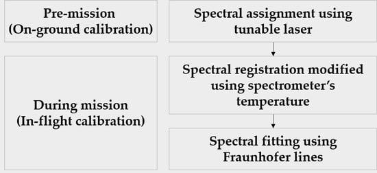
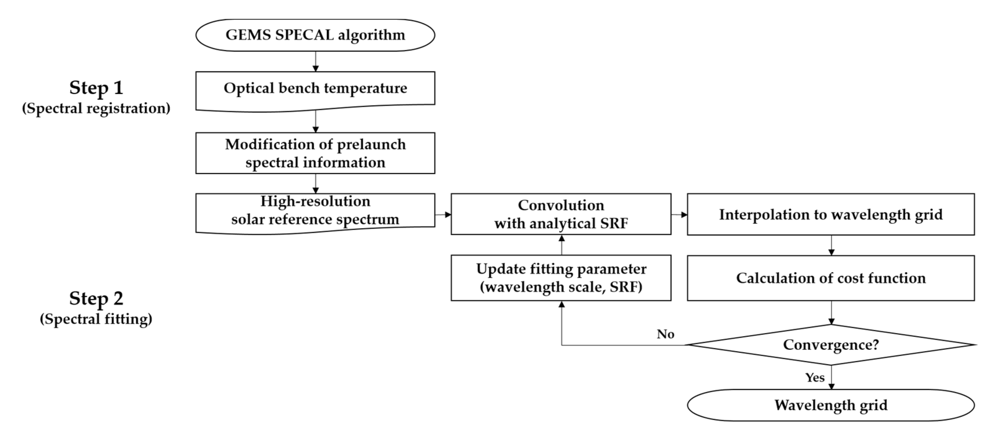
To account and correct for the spectral deviation occurring in the space, SPECAL is designed to run in two steps during the GEMS mission as shown in Figure 1. The first step assigns wavelength using prelaunch and early orbit calibration data, which are measured at various temperatures covering the full range of spectrometer temperatures [16]. As shown in Equation (1), the first-step wavelength λ is obtained by adjusting λi, wavelength determined by on-ground test, as a function of temperature difference between in-orbit (TOPB) and on-ground (TOPB_ref) with the pre-determined polynomial coefficients of α0 and α1.
The first step is straightforward and fast, but previous studies have shown that its calibration accuracy is insufficient for level 2 products such as ozone profiles [14,15,16,17]. The uncertainty induced in the first step could be large enough and propagate to become an unacceptable source of errors in DOAS-type retrieval algorithms. Therefore, additional SPECAL process and a second step are necessary for the required level 1b data quality.
The second step of SPECAL uses cross-correlation [14], which fits the spectral features of the measured solar irradiance or radiance to those of accurately known high-resolution reference spectrum. It iteratively finds spectral scale parameters (e.g., spectral shift and squeeze) based on nonlinear least-square fitting, optionally with iterative damping constraints (i.e., the Levenberg–Marquardt method) [28]. Using the on-ground calibration data as a first estimate, the algorithm calculates Jacobians with respect to these parameters and the cost function. The wavelength scale is optimally estimated by updating the spectral fitting parameters until the cost function is minimized and the parameters converge. As a reference spectrum for comparison with GEMS measurements, the high-resolution solar reference irradiance spectrum is convolved with the analytical SRF based on the on-ground calibration result. Several high-resolution reference spectra are currently available for the GEMS spectral range. Section 3.4 gives a detailed sensitivity analysis for the use of different reference spectra for SPECAL.
Equation (2) shows the baseline formula for the spectral fitting, representing a formula to estimate the simulated irradiance (IM(λ)) using the reference solar irradiance convolved by fitting parameters.
Here, IR(λ) is the reference spectrum modulated and convolved from a high-resolution solar reference spectrum, IH(λ) with an analytic SRF, , as shown in Equation (3), while dG is the initial wavelength scale (λ) minus its averaged value (λavg), and Si (i = 0–3) are the coefficients of a third-order scaling polynomial for IR(λ).
Thus, the second step of SPECAL iteratively varies dG until the estimated IR(λ) with the measured IM(λ) are converged. The weighting functions for each fitting parameter are calculated at each iteration either analytically or using finite differences, and then used for the inversion. In Equation (2), The Earth radiance is affected by atmospheric absorption (especially by ozone) and scattering (Ring effect, and Rayleigh and Mie scattering). Additional fitting parameters are included for the SPECAL of radiances [15] (not presented in this paper).
As shown in Equations (2) and (3), SRF plays the key role in determining estimated IR(λ), and thus in the overall fitting procedure. To safely represent any changes in the SRF characteristics during the operation in space, the fitting algorithm also includes additional SRF parameters (i.e., shape, width, and asymmetry). For the GEMS SRF mode, we use empirical numerical functions such as asymmetric and broadened Gaussian [22] or Super-Gaussian [29], which are widely used and proven in prior studies [24,30,31], for the spectral fitting process.
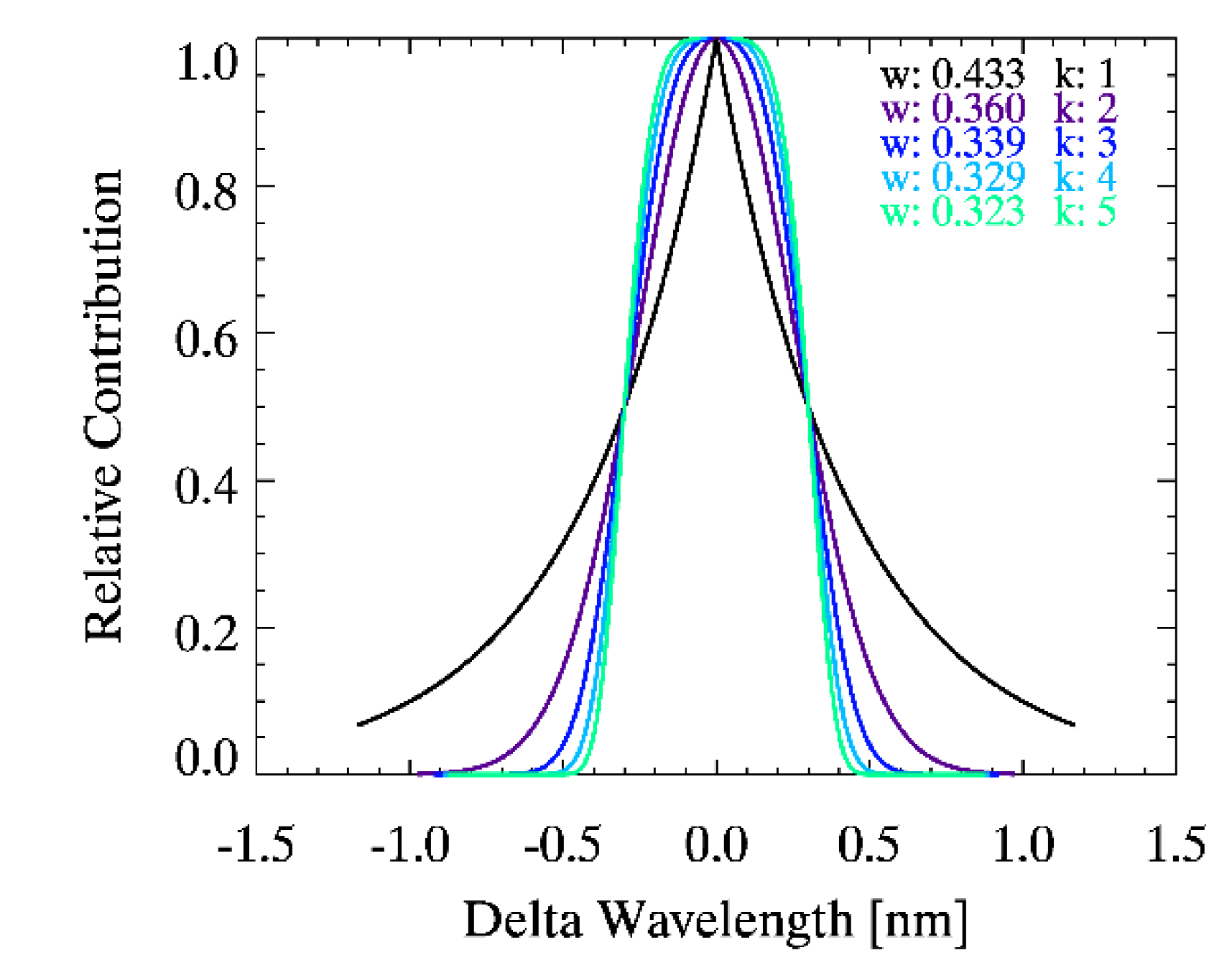
To examine the sensitivities of SPECAL to the shape parameters, we used the asymmetric Super-Gaussian (ASG) function [28] as shown in Equation (4).
where k and w are independent parameters that determine the shape and width of f(λ), respectively, Γ is the gamma function, and aw and ak are additional asymmetry parameters [28]. When k is 2, the ASG function becomes a Gaussian function. For k < 2, the function has a more pointed shape with longer tails.
Shift (Ch) and squeeze (Cq) are generally used to represent the actual wavelength shift relative to the initial wavelength scale. Shift describes linear changes in the wavelength scale, while squeeze denotes non-linear changes. Thus, the wavelength change for each detector pixel is different in the presence of a squeeze. The wavelength change due to shift and squeeze is modeled as follows:
Based on Equation (5), the actual wavelength grid is the same as the initial grid when the shift is zero and the squeeze is 1 (i.e., no squeeze).
On the other hand, there are frequent disadvantages to utilizing the squeeze parameter for the quantification of actual wavelength changes. When an algorithm calculates a value for squeeze in certain fitting windows, understanding the degree of change in the whole wavelength range is not straightforward. Additionally, it might not be realistic to separate wavelength changes into a single shift and squeeze, considering the actual wavelength assignment is non-linear and often parameterized as a fifth- to over tenth-degree polynomial [32]. Therefore, for simplicity in understanding wavelength changes and for more straightforward utilization in retrieval processes, it is often the case that only the shift parameter is fitted. To describe the changes over the entire observational wavelength range with shift only, we introduced high-order shift coefficients (here, fifth-order polynomial) as shown in Equation (6), to sufficiently account for the non-linear variation of the wavelength change:
2.4. Sensitivity Tests
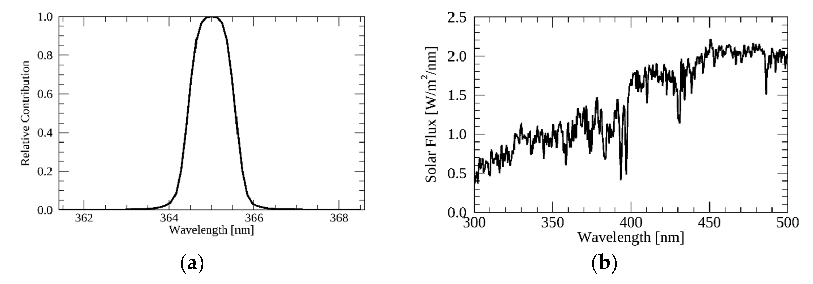
A series of sensitivity tests was conducted to estimate the performance of the algorithm with respect to uncertainties in the fitting parameters. As the GEMS instrument is in the commissioning phase, observed spectra are currently not available; therefore we used a synthetic spectrum prepared by convolving a high-resolution solar reference spectrum with the measured GEMS SRF during the laboratory calibration, with artificially perturbed wavelength parameters over the spectral range (300 to 500 nm). The synthetic spectrum also includes expected measurement noise, calculated based on the noise model of GEMS. Figure 2 shows such a synthetic spectrum along with the measured SRF at a nominal wavelength of 365 nm. For more realistic and precise error estimation of SPECAL, detailed spectral parameters were considered, including signal-to-noise ratio (SNR), wavelength scale parameter, fitting window, SRF, and high-resolution solar reference spectrum. The test results for each spectral parameter are described in the following subsections. The algorithm is not meaningfully sensitive to the SNR; therefore, the results for SNR are not presented here.
The sensitivity test compares the spectral parameters estimated by SPECAL algorithm with the perturbed spectral parameters used to generate the synthetic spectrum. The prepared synthetic spectra, including wavelength perturbations and radiometric uncertainty, are assumed to be realistic GEMS solar measurements. Table 2 summarizes the input and retrieved parameters, revealing that the retrieved values are consistent with the given perturbations within the expected uncertainty of the spectral parameters. The performance of the algorithm is also evaluated using mean bias (Bλ) and root-mean-squared deviation (RMSD, Sλ) between the known (true value before perturbation) and retrieved wavelength registration. The calculated Bλ and Sλ are less than the required spectral accuracy of GEMS (i.e., 0.002 nm), also shown in Table 2. Although SPECAL produces optimal values for the given simulated spectrum and measurement, there are possibilities of additional uncertainties which are analyzed and quantified in the next section.
3. Results and Discussion
3.1. Wavelength Scale Parameter
The wavelength change compared with the initial wavelength scale is represented using wavelength scale parameters such as shift, squeeze, and shift polynomials. To examine the calibration’s sensitivity to the wavelength scale parameters, we applied the parameters differently to the synthetic data and the SPECAL algorithm. For the sensitivity study, we carefully selected the arbitrary perturbation (Cq = 0.005, Ch1 = 0.001, Ch2 = 0.0002) to reflect realistic spectral shift due to the nonlinear optical temperature gradient, which results in inhomogeneous spectral change up to a few pixels. The algorithm’s performance corresponding to the shift and squeeze parameters or the shift polynomial is compared for the whole GEMS observational wavelength range.
The obtained cost function and fitted parameter values indicate that the outputs are consistent with the simulated inputs when the algorithm uses a shift polynomial rather than shift and squeeze (Table 3). The algorithm fitting a shift polynomial successfully follows the simulated wavelength change that consists of shift and squeeze, whereas the opposite case does not. As the squeeze parameter is related to the first-order term of the shift polynomial (Equations (4) and (5)), fitting a shift and squeeze is not able to correctly capture the actual wavelength variation due to the large spectral shifts. Therefore, the approaches using shift and squeeze [13,14,15,18] are insufficient to represent the relatively nonlinear features and can thus lead to the apparent residual mismatch with the reference spectrum. Furthermore, fitting a polynomial to account for high-order shifts might converge more quickly with fewer iterations than fitting with shift and squeeze. When considerable nonlinear wavelength changes are expected, such as when a sufficient number of fitting radiances are required, it is better to apply the high-order shift parameters for the spectral fitting procedure.
3.2. Fitting Window
Although high-order shifter parameters are recommended, a fitting window that is too wide for the wavelength range applicable to the calibration can introduce unacceptable fitting errors in the significant dynamic range of radiance measurements; the errors can be up to about three orders of magnitude in the GEMS spectral domain (i.e., 300–500 nm) [16]. Therefore, if the fitting can be performed sufficiently quickly, it is better to perform SPECAL over several narrow fitting windows across the spectral range rather than fitting a shift polynomial over the entire (single) range. Fitting with multiple sub-windows allows detailed monitoring of the detector response and provides L1b data with sufficient accuracy for specific trace gas retrieval. For each selected sub-window (e.g., 10 or 15 nm), using a single shift parameter (Ch) is appropriate, as nonlinear spectral change is typically negligible in this case. The derived shift at each sub-window is then fitted to a polynomial as a function of wavelength to determine the amount of shift for every spectral pixel [14]. The number of sub-windows should be sufficient to obtain reliable results compared with the use of shift polynomials for the entire window. However, increasing the number of windows with a single fit parameter increases the numerical cost for the algorithm to converge. A further consideration is that the polynomial approach applied to derive the shift for each CCD pixel could affect SPECAL’s accuracy. Changing the fitting windows while keeping a constant wavelength range (for example, 400–450 nm to 410–460 nm) has an insignificant effect on the calculation time. Therefore, we focused on the effects of different numbers of fitting windows on the calculation time and algorithm performance.
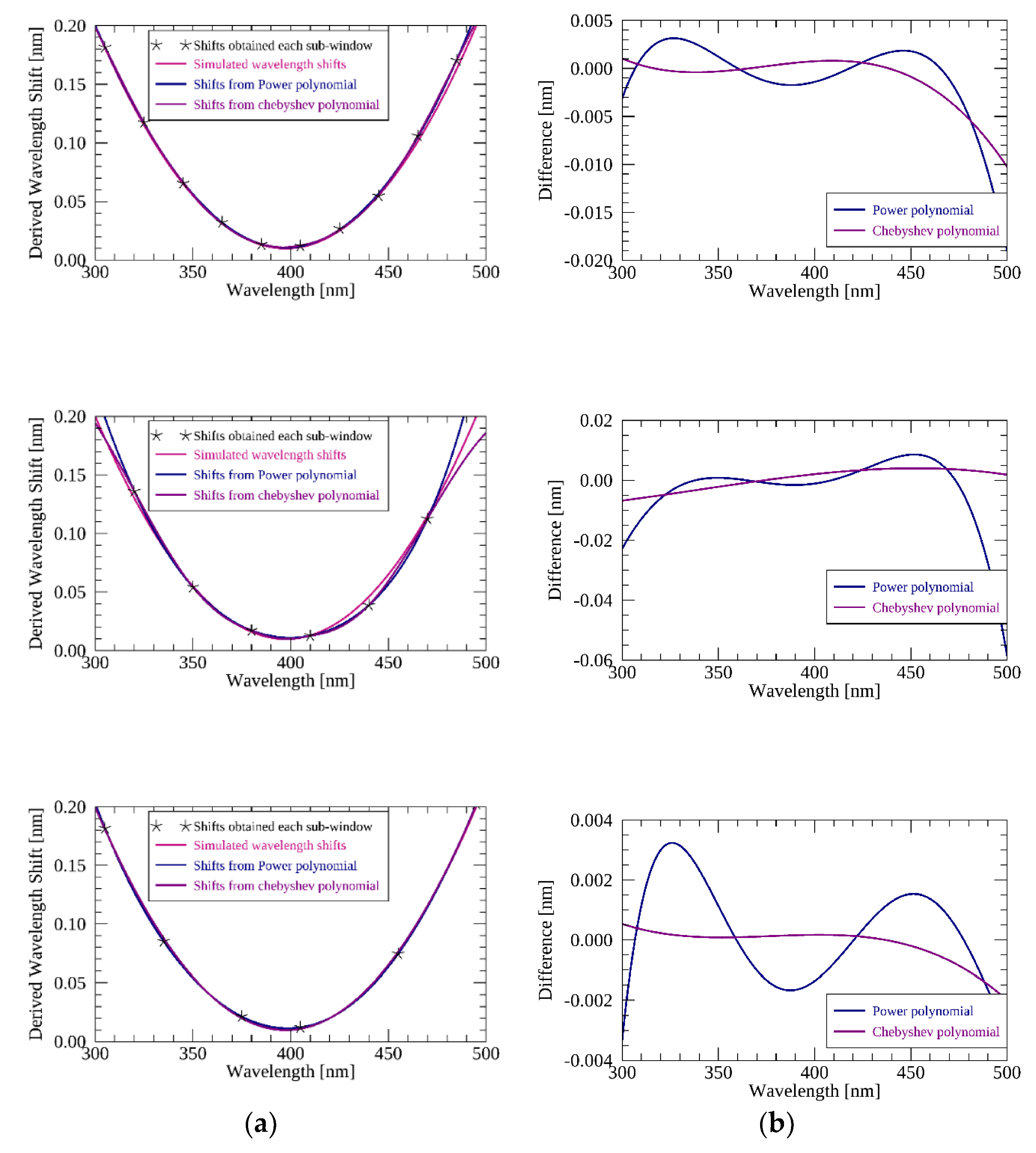
Here, the effects of two types of polynomial (power and Chebyshev) are compared. The calibration is repeatedly performed over 6 to 10 small sub-windows selected within the GEMS coverage. Results are shown in Figure 3. The magenta lines are the applied simulated wavelength shifts (Ch0: 0.01, Ch1: 0.0001, Ch2: 0.00002), and asterisks are fitted shifts from each fitting window. Purple and blue lines represent the derived wavelength shifts based on Chebyshev and power polynomials, respectively. The figure’s right panel (b) shows that the shifts obtained using Chebyshev polynomials achieve better consistency with the simulated wavelength shift than the power polynomials. Table 4 lists the corresponding mean bias and RMSD for each fitting window. The results for fitting windows 1 and 2 show that a sufficient number of fitting windows is required to reflect the actual wavelength variations for the whole wavelength range. Nevertheless, using fewer fitting windows is numerically efficient, particularly when wavelength variability can be explained by low-order nonlinearity that satisfies Nyquist sampling frequency.
Comparing the results of fitting windows 2 and 3, with the same number of sub-windows, shows the importance of the locations of the sub-windows. It is necessary to optimize not only the number of sub-windows but also their ranges. The behavior of the actual wavelength changes observed during the mission will contribute to the selection and optimization of the fitting windows. In addition, the wavelength shift derived for each spectral pixel could depend on the chosen polynomial. While the algorithm’s performance meets the requirement for GEMS using either Chebyshev or power polynomials, the former gives better agreement regardless of the fitting window. (For fitting window 2, Bλ and Sλ of the power polynomial are 2.71 and 15.8, respectively, and 1.29 and 5.44, respectively, for the Chebyshev polynomial). Because the power polynomial used for expansion to the entire wavelength range [15,16,17] becomes unreliable near the lower and upper end of the wavelength band (i.e., below 310 nm, above 490 nm), it is not advisable to use the power polynomial for the SPECAL of sub-windows.
3.3. Spectral Response Function
Figure 4 shows results for the sensitivity tests of the SRF with five ASG functions. Each synthetic spectrum is then derived by convolution of a high-resolution solar reference spectrum. First, we apply the algorithm to synthetic irradiances convolved with different SRFs in Table 5, without including SRF fitting. The algorithm assumes a fixed symmetric Gaussian SRF. The cost function and calibration results for several synthetic spectra with different SRFs are summarized in Table 5. The algorithm’s sensitivity increases with the changes of shape (k) and width (w) of the SRF. The results indicate that the algorithm is significantly more sensitive to the shape (skewness) of the SRF than its width SRF. This is because the width of the SRF is related to the resolution of the spectrum, while its shape greatly determines the representative spectral characteristics. The algorithm fails to meet the requirements of GEMS, except when the simulated SRF is fully Super-Gaussian (k = 2). Therefore, the uncertainty of the shape of the SRF is a decisive factor determining the algorithm’s accuracy.
Nevertheless, in-flight characterization of the SRF and its variation/correction can be well described using an empirical function such as ASG, as it can simultaneously fit the shape and width of the SRF with sufficient accuracy [28,29,30]. Table 6 shows that the SPECAL algorithm, with fitted SRF parameters, successfully estimates the actual SRF except for the unrealistic change of shape and width of the SRF (when it changes from a fully Super-Gaussian to a Triangular model). The listed biases between the input and derived SRFs from the algorithm (denoted as Bf) are less than 0.1%. The calibration accuracy is improved by up to ten times compared to the previous algorithm [19] without a noticeable difference in the computational time. Furthermore, retrieval of in-orbit SRF using analytical function is useful even if the prelaunch SRF is not well known. Spectral convolution of the high-resolution solar reference spectrum and interpolation of the SRF to a different wavelength grid are the main factors affecting the computation time. As GEMS observes the Sun during the night, there is enough time to calibrate the data by deriving the SRF. However, when variations in the SRF are not significant in-orbit, using a pre-computed reference spectrum convolved with a known nominal SRF (characterized during commissioning) can reduce the numerical cost.
We also perform a similar sensitivity study for the two asymmetric factors (aw and ak) when the shape and width parameters (w and k) are fixed as 0.360 and 2, respectively. The SRF’s asymmetry is known to closely correlate with shift (Ch0) [19], which is quantitatively confirmed in our algorithm results. Both asymmetry parameters are similarly correlated with the shift parameter, shown as Table 7. Their variation effectively leads to a linear wavelength change. Therefore, increasing asymmetry in the SRF further changes the wavelength shift (i.e., Ch0 varies from 0.001 to 0.081).
3.4. High-Resolution Solar Reference Spectrum
The high-resolution solar reference spectrum is critical to spectral and radiometric calibrations for satellite-based instruments. Specific applications include determination of instrument SRFs, accurate radiative transfer calculations, and Ring effect corrections [33,34,35,36,37]. There are various solar reference spectra with different radiometric accuracy, spectral resolution, wavelength range, and other spectral characteristics. To make an appropriate selection for GEMS, it is necessary to consider the radiometric and spectral uncertainty of each reference spectrum. GEMS has the following requirements: the absolute radiometric uncertainty must be less than the GEMS radiometric accuracy (4%); the resolution of the solar reference spectrum must be higher than the GEMS resolution (0.6 nm); and, finally, fully Nyquist sampled spectra are preferred.
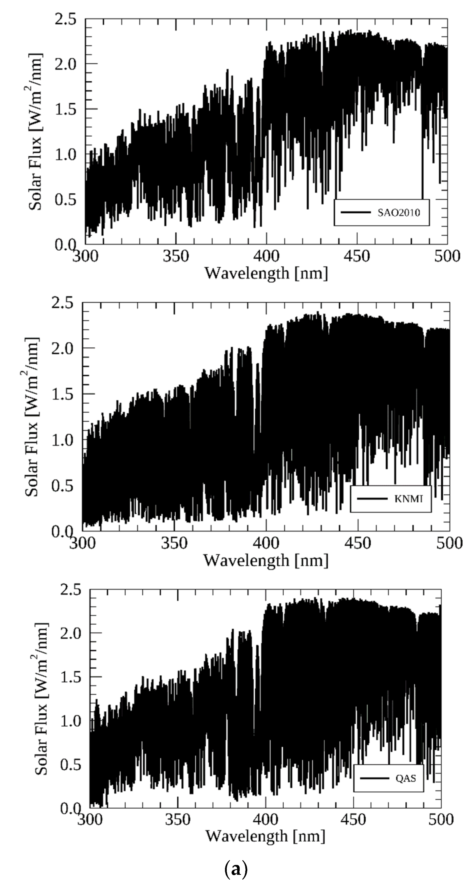
Compared to the numerous low-resolution spectra, few suitable higher-resolution spectra are available due to the limited observations. Here, three candidates are considered for the GEMS solar reference. One is the Royal Netherlands Meteorological Institute (KNMI) spectrum, developed by Dobber et al., (2008) [34], which is utilized as the solar reference spectrum for the calibrating OMI instrument. Another is the SAO2010 spectrum provided by Chance and Kurucz [36], an updated version of the SAO96 [33] that had been widely used in heritage satellite mission programs. The final potential spectrum has recently been determined from ground-based measurements by the Quality Assurance of Spectral Ultraviolet Measurements in Europe spectroradiometer and a Fourier transform spectroradiometer (hereafter referred to as the QAS spectrum) [37]. Figure 5a shows each spectrum over the GEMS observational wavelength range.
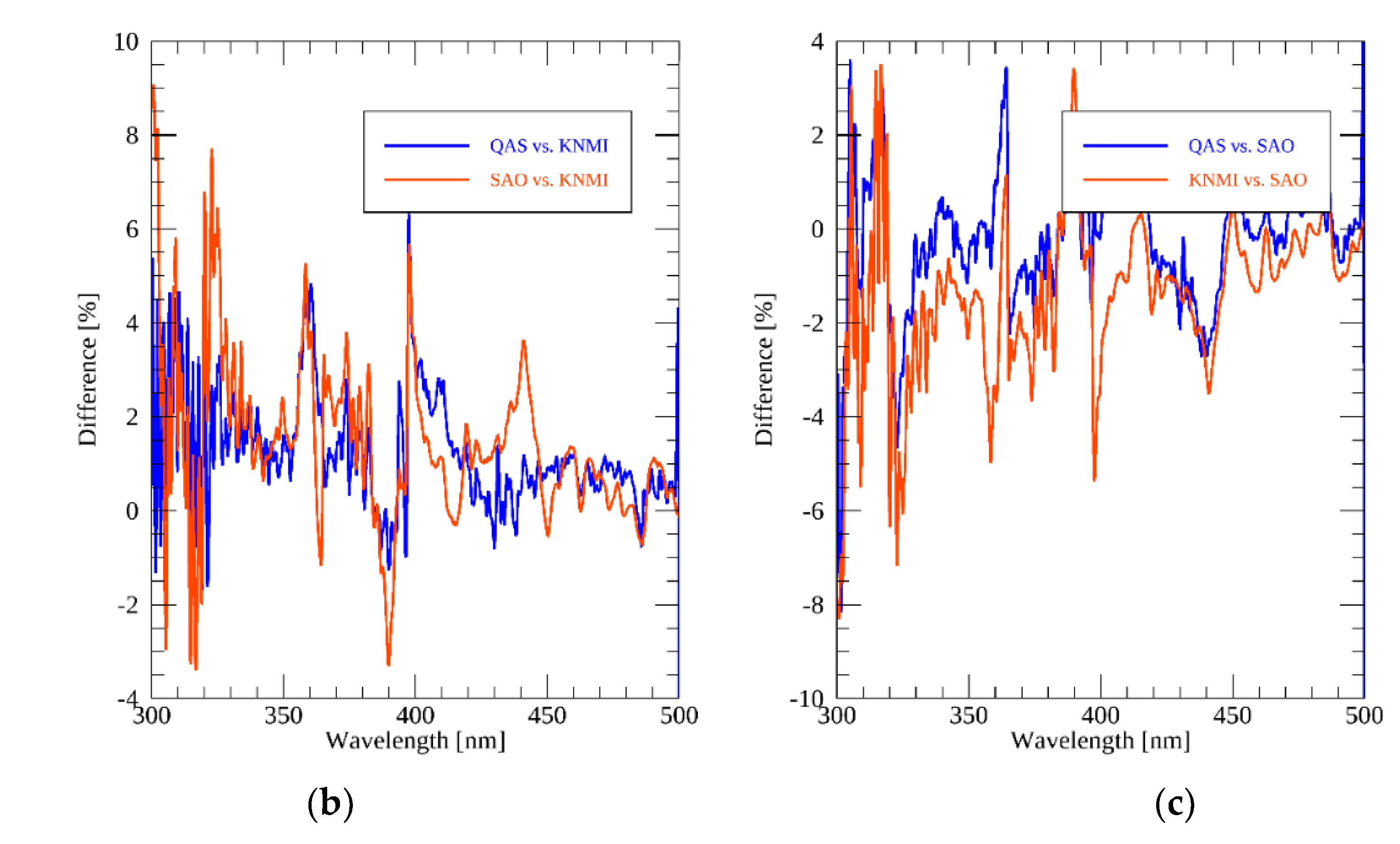
To characterize the differences associated with these spectra, they are compared at the spectral resolution and range of GEMS, as shown in Figure 5b,c. Each spectrum is known to have similar radiometric accuracy (uncertainty of less than 4% for the GEMS observational range), and the average difference among them is less than 1.4%. However, it should be noted that there are significant differences of up to 8% at shorter wavelengths (see Figure 5). As the hyperspectral solar reference irradiances considered here are composite spectra from ground-based and/or balloon-based measurements, they might contain atmospheric absorption features [14]. The large radiative differences below 310 nm, for example, are likely related to ozone absorption. In addition, as a result of these radiometric uncertainties, SPECAL is significantly sensitive to the choice of high-resolution solar reference spectrum, as shown in Table 8.
The calibration accuracy using the QAS spectrum is lower than that achieved with the SAO2010 and KNMI spectra. The minimum chi-squared, mean bias, and RMSD values (2.45, 6.59, and 3.81, respectively) are larger than those for the other spectra. The shift values (Ch0 and Ch1) retrieved in the QAS test also indicate that the absolute wavelength calibration of the QAS itself is insufficient compared with other sources of solar irradiances. The expected value is 0.01 nm for Ch0, but the output of 0.009 nm indicates a residual of 0.001. Second, using different high-resolution solar reference spectra for the derivation of the synthetic data and simulated spectrum (reference spectrum) significantly degrades SPECAL’s performance. The retrieved shift parameter shows an additional wavelength shift of up to 0.017 nm with the cost function increased by over an order of magnitude when using KNMI and QAS. This unacceptable calibration result arises owing to radiometric uncertainties between the solar reference spectra. However, as the SPECAL error is larger with KNMI and QAS compared to SAO and KNMI, and the calibration result is sensitive not only to the radiometric accuracy [14,19,25] but also to the spectral accuracy of the solar reference data. Therefore, to further improve SPECAL, proper choice of the solar reference spectrum is of critical importance. The optimal solar reference spectrum for GEMS is to be determined using on-orbit solar measurements during the instrument’s in-orbit tests.
4. Conclusions
A spectral calibration algorithm for GEMS is presented here. To achieve sufficient accuracy for level 2 products, the calibration is performed using spectral fitting. The algorithm was designed to minimize the differences between the simulated reference spectrum (derived by convolving a high-resolution solar reference spectrum with the instrument SRF) and the spectrum measured by GEMS. To estimate the performance of the algorithm, the effects of several spectral fitting parameters on the calibration were examined using cost function and fitting residual.
Within the expected wavelength variation (up to a few pixels), the algorithm showed acceptable performance (accuracy better than 0.002 nm) to the expected uncertainties associated with most of spectral parameters, such as wavelength perturbation and signal-to-noise ratio. Such a satisfactory performance is possible mainly due to the inclusion of additional fitting parameters of spectral scales (shift, squeeze, and high order shifts) and SRF (width, shape, and asymmetry).
Here, it is clearly shown that the choice of the high-resolution solar reference spectrum and uncertainties in the in-flight SRF are critical to the performance of spectral calibration. The sensitivity to the SRF is expected to be mitigated by using the derived in-flight SRFs using analytical functions or modification of prelaunch SRFs. On the other hand, the radiometric disagreement between the high-resolution solar reference spectra is non-negligible in the GEMS observational range, especially below 310 nm; therefore, selecting the optimal solar reference spectrum is vital for better calibration performance. Indeed, the estimated uncertainty of the spectral calibration algorithm (less than 0.8%) is primarily contributed by the sensitivity to the high-resolution solar reference spectrum (about 0.7%). Furthermore, the current candidate reference spectra for GEMS might include some atmospheric absorption features; thus, further improvements are possible for spectral calibration after updating the current references or using a pure high-resolution solar spectrum measured from space.
As GEMS measures solar irradiance once per day during the night, much earlier than the normal Earth radiance observation begins, the algorithm could afford a sufficient number of fitting parameters, while the number of parameters for radiance measurements is limited due to the numerical cost. Hence, the operational spectral calibration algorithm for solar irradiance is designed to include accurate SRF fitting parameters together with shift polynomials or shifts based on carefully selected narrow fitting windows. As GEMS is known to have a very stable optical bench temperature and, thus, the wavelength variation during the daytime is expected to be small. Therefore, wavelengths of level 1b radiances are determined by modifying the wavelengths obtained from solar irradiances. The accuracy of the spectral calibration for radiances could further be improved by the use of radiative transfer model. Current principal component analysis and machine-learning-based hyperspectral radiative transfer models could derive entire high-resolution radiances from a small number of radiances [38,39]. These fast models with modules for Jacobian calculation have potential to perform a real-time spectral fitting of radiance. It is possible to produce the reference spectrum and fitting parameters at each iteration step for better calibration result.
Although spectral calibration for solar observations includes the parameters of SRF used to convolve the high-resolution solar reference spectrum, it incurs huge computational cost. Therefore, the application of a pre-derived reference spectrum convolved with a known nominal SRF is possible when the amount of change in the SRF during the mission is insignificant. The effect of applying wavelength shift can be linearized as a shift spectrum and then included as a pseudo absorber spectrum; such linearization can also further expedite the fitting process. These approaches will therefore be investigated during in-orbit tests. After the commissioning phase, calibrated GEMS measurements are expected to be released for the public at the end of 2020.
5. Patent
There is a Korea patent registration (10-2100545) resulting from this work.
Author Contributions
M.K. led manuscript writing, contributed to research design, and analyzed the results. M.-H.A. supervised this study, contributed to conceiving the idea and writing, and serves as the corresponding author. X.L. contributed to the research design and manuscript writing. U.J. contributed to manuscript writing. J.K. contributed to the discussion of the results. All authors have read and agreed to the published version of the manuscript.
Funding
This work is supported by the Korea Ministry of Environment (MOE) as “Public Technology Program based on Environmental Policy (2017000160002)”.
Conflicts of Interest
The authors declare no conflict of interest.
References
- Lee, S.; Ahn, M.; Chung, S. Atmospheric Profile Retrieval Algorithm for Next Generation Geostationary Satellite of Korea and Its Application to the Advanced Himawari Imager. Remote Sens. 2017, 9, 1294. [Google Scholar] [CrossRef] [Green Version]
- Kim, J.; Jeong, U.; Ahn, M.; Kim, J.; Park, R.; Lee, H.; Song, C.; Choi, Y.; Lee, K.; Yoo, J.; et al. New Era of Air Quality Monitoring from Space: Geostationary Environment Monitoring Spectrometer (GEMS). Bull. Am. Meteorol. Soc. 2020, 101, E1–E2. [Google Scholar] [CrossRef] [Green Version]
- Choi, W.J.; Moon, K.; Yoon, J.; Cho, A.; Kim, S.; Lee, S.; Ko, D.H.; Kim, J.; Ahn, M.H.; Kim, D.; et al. Introducing the Geostationary Environment Monitoring Spectrometer. J. Appl. Remote. Sens. 2019, 13, 019901. [Google Scholar] [CrossRef] [Green Version]
- Kim, M.; Kim, J.; Torres, O.; Ahn, C.; Kim, W.; Jeong, U.; Go, S.; Liu, X.; Moon, J.K.; Kim, D.-R. Optimal Estimation-Based Algorithm to Retrieve Aerosol Optical Properties for GEMS Measurements over Asia. Remote Sens. 2018, 10, 162. [Google Scholar] [CrossRef] [Green Version]
- Kwon, H.-A.; Park, R.J.; González Abad, G.; Chance, K.; Kurosu, T.P.; Kim, J.; De Smedt, I.; Van Roozendael, M.; Peters, E.; Burrows, J. Description of a formaldehyde retrieval algorithm for the Geostationary Environment Monitoring Spectrometer (GEMS). Atmos. Meas. Tech. 2019, 12, 3551–3571. [Google Scholar] [CrossRef] [Green Version]
- Chong, H.; Lee, S.; Kim, J.; Jeong, U.; Li, C.; Krotkov, N.; Nowlan, C.; Al-Saadi, J.; Janz, S.; Kowalewski, M.; et al. High-resolution mapping of SO2 using airborne observations from the GeoTASO instrument during the KORUS-AQ field study: PCA-based vertical column retrievals. Remote Sens. Environ. 2020, 241, 111725. [Google Scholar] [CrossRef]
- Dobber, M.; Dirksen, R.; Voors, R.; Mount, G.H.; Levelt, P. Ground-Based Zenith Sky Abundances and in Situ Gas Cross Sections for Ozone and Nitrogen Dioxide with the Earth Observing System Aura Ozone Monitoring Instrument. Appl. Opt. 2005, 44, 2846–2856. [Google Scholar] [CrossRef] [Green Version]
- Cai, Z.; Liu, Y.; Liu, X.; Chance, K.; Nowlan, C.R.; Lang, R.; Munro, R.; Suleiman, R. Characterization and Correction of Global Ozone Monitoring Experiment 2 Ultraviolet Measurements and Application to Ozone Profile Retrievals. J. Geophys. Res. 2012, 117. [Google Scholar] [CrossRef]
- De Smedt, I.; Van Roozendael, M.; Stavrakou, T.; Müller, J.; Lerot, C.; Theys, N.; Valks, P.; Hao, N.; Van Der, A.R. Improved Retrieval of Global Tropospheric Formaldehyde Columns from GOME-2/MetOp-A Addressing Noise Reduction and Instrumental Degradation Issues. Atmos. Meas. Tech. 2012, 5, 2933–2949. [Google Scholar] [CrossRef] [Green Version]
- Brewer, A.; McElroy, C.; Kerr, J. Nitrogen Dioxide Concentrations in the Atmosphere. Nature 1973, 246, 129–133. [Google Scholar] [CrossRef]
- Platt, U.; Perner, D. Measurements of Atmospheric Trace Gases by Long Path Differential UV/Visible Absorption Spectroscopy. In Optical and Laser Remote Sensing; Killinger, D.K., Mooradian, A., Eds.; Springer: Berlin/Heidelberg, Germany, 1983; pp. 97–105. [Google Scholar]
- Stutz, J.; Platt, U. Numerical Analysis and Estimation of the Statistical Error of Differential Optical Absorption Spectroscopy Measurements with Least-Squares Methods. Appl. Opt. 1996, 35, 6041–6053. [Google Scholar] [CrossRef] [PubMed] [Green Version]
- Caspar, C.; Chance, K. GOME Wavelength Calibration using Solar and Atmospheric Spectra. In Proceedings of the Third ERS Symposium on Space at the Service of our Environment, Florence, Italy, 14 March 1997; pp. 609–614. [Google Scholar]
- Van Geffen, J.H. Wavelength Calibration of Spectra Measured by the Global Ozone Monitoring Experiment: Variations Along Orbits and in Time. Appl. Opt. 2004, 43, 695–706. [Google Scholar] [CrossRef] [PubMed]
- Van Geffen, J.H.; van Oss, R.F. Wavelength Calibration of Spectra Measured by the Global Ozone Monitoring Experiment by use of a High-Resolution Reference Spectrum. Appl. Opt. 2003, 42, 2739–2753. [Google Scholar] [CrossRef] [PubMed]
- Voors, R.; Dobber, M.; Dirksen, R.; Levelt, P. Method of Calibration to Correct for Cloud-Induced Wavelength Shifts in the Aura Satellite’s Ozone Monitoring Instrument. Appl. Opt. 2006, 45, 3652–3658. [Google Scholar] [CrossRef]
- Kuhlmann, G.; Hueni, A.; Damm, A.; Brunner, D. An Algorithm for in-Flight Spectral Calibration of Imaging Spectrometers. Remote Sens. 2016, 8, 1017. [Google Scholar] [CrossRef] [Green Version]
- Seftor, C.; Jaross, G.; Kowitt, M.; Haken, J.; Flynn, L. Post-launch performance of the Suomi NPP Ozone Mapping and Profiler Suite (OMPS) nadir sensors. J. Geophys. Res. Atmos. 2013, 119, 4413–4428. [Google Scholar] [CrossRef] [Green Version]
- Ahn, M.; Kang, M.; Liu, X.; Kim, J. A Sensitivity Study for the Calibration of Hyperspectral Spectrometer on Board the Geostationary Multipurpose Satellite of Korea. In Proceedings of the Third International Conference on Remote Sensing and Geoinformation of the Environment, Paphos, Cyprus, 19 June 2015. [Google Scholar]
- Ceamanos, X.; Douté, S. Spectral Smile Correction of CRISM/MRO Hyperspectral Images. IEEE Trans. Geosci. Remote Sens. 2010, 48, 3951–3959. [Google Scholar] [CrossRef]
- Dirksen, R.; Dobber, M.; Voors, R.; Levelt, P. Prelaunch Characterization of the Ozone Monitoring Instrument Transfer Function in the Spectral Domain. Appl. Opt. 2006, 45, 3972–3981. [Google Scholar] [CrossRef]
- Liu, C.; Liu, X.; Kowalewski, M.G.; Janz, S.J.; Gonzal Abad, G.; Pickering, K.E.; Chance, K.; Lamsal, L.N. Characterization and Verification of ACAM Slit Functions for Trace-Gas Retrievals during the 2011 DISCOVER-AQ Flight Campaign. Atmos. Meas. Tech. 2015, 8, 751–759. [Google Scholar] [CrossRef] [Green Version]
- Munro, R.; Lang, R.; Klaes, D.; Poli, G.; Retscher, C.; Lindstrot, R.; Huckle, R.; Lacan, A.; Grzegorski, M.; Holdak, A. The GOME-2 Instrument on the Metop Series of Satellites: Instrument Design, Calibration, and Level 1 Data processing–an Overview. Atmos. Meas. Tech. 2016, 9, 1279–1301. [Google Scholar] [CrossRef] [Green Version]
- Sun, K.; Liu, X.; Huang, G.; Abad, G.G.; Cai, Z.; Chance, K.; Yang, K. Deriving the Slit Functions from OMI Solar Observations and its Implications for Ozone-Profile Retrieval. Atmos. Meas. Tech. 2017, 10, 3677–3695. [Google Scholar] [CrossRef] [Green Version]
- Noël, S.; Bramstedt, K.; Bovensmann, H.; Gerilowski, K.; Burrows, J.; Standfuss, C.; Dufour, E.; Veihelmann, B. Quantification and Mitigation of the Impact of Scene Inhomogeneity on Sentinel-4 UVN UV-VIS Retrievals. Atmos. Meas. Tech. 2012, 5, 1319–1331. [Google Scholar] [CrossRef] [Green Version]
- Ko, D.H.; (Korea Aerospace Research Institute, Yuseong-Gu, Daejeon, Korea). Personal communication, 2018.
- Giesen, P.; Folgering, E. Design Guidelines for Thermal Stability in Opto-Mechanical Instruments. In Proceedings of the SPIE’s 48th Annual Meeting, San Diego, CA, USA, 27 October 2003. [Google Scholar]
- Rodgers, C.D. Levenberg-Marqurdt method. In Inverse Methods for Atmospheric Sounding: Theory and Practice; Taylor, F.W., Ed.; World Scientific Publishing Co. Pte. Ltd.: Singapore, 2000; Volume 2, pp. 92–99. [Google Scholar]
- Beirle, S.; Lampel, J.; Lerot, C.; Sihler, H.; Wagner, T. Parameterizing the Instrumental Spectral Response Function and its Changes by a Super-Gaussian and its Derivatives. Atmos. Meas. Tech. 2017, 10, 581–598. [Google Scholar] [CrossRef] [Green Version]
- Sun, K.; Liu, X.; Nowlan, C.R.; Cai, Z.; Chance, K.; Frankenberg, C.; Lee, R.A.; Pollock, R.; Rosenberg, R.; Crisp, D. Characterization of the OCO-2 Instrument Line Shape Functions using on-Orbit Solar Measurements. Atmos. Meas. Tech. 2017, 10, 939–953. [Google Scholar] [CrossRef] [Green Version]
- Hamidouche, M.; Lichtenberg, G. In-Flight Retrieval of SCIAMACHY Instrument Spectral Response Function. Remote Sens. 2018, 10, 401. [Google Scholar] [CrossRef] [Green Version]
- Kleipool, Q.; Ludewig, A.; Babić, L.; Bartstra, R.; Braak, R.; Dierssen, W.; Dewitte, P.; Kenter, P.; Landzaat, R.; Leloux, J.; et al. Pre-Launch Calibration Results of the TROPOMI Payload on-Board the Sentinel-5 Precursor Satellite. Atmos. Meas. Tech. 2018, 11, 6439. [Google Scholar] [CrossRef] [Green Version]
- Chance, K.V.; Spurr, R.J. Ring Effect Studies: Rayleigh Scattering, including Molecular Parameters for Rotational Raman Scattering, and the Fraunhofer Spectrum. Appl. Opt. 1997, 36, 5224–5230. [Google Scholar] [CrossRef] [Green Version]
- Thuillier, G.; Hersé, M.; Foujols, T.; Peetermans, W.; Gillotay, D.; Simon, P.; Mandel, H. The Solar Spectral Irradiance from 200 to 2400 Nm as Measured by the SOLSPEC Spectrometer from the ATLAS and EURECA Missions. Sol. Phys. 2003, 214, 1–22. [Google Scholar] [CrossRef]
- Dobber, M.; Voors, R.; Dirksen, R.; Kleipool, Q.; Levelt, P. The High-Resolution Solar Reference Spectrum between 250 and 550 Nm and its Application to Measurements with the Ozone Monitoring Instrument. Sol. Phys. 2008, 249, 281–291. [Google Scholar] [CrossRef] [Green Version]
- Chance, K.; Kurucz, R. An Improved High-Resolution Solar Reference Spectrum for Earth’s Atmosphere Measurements in the Ultraviolet, Visible, and Near Infrared. J. Quant. Spectrosc. Radiat. Transf. 2010, 111, 1289–1295. [Google Scholar] [CrossRef]
- Gröbner, J.; Kröger, I.; Egli, L.; Hülsen, G.; Riechelmann, S.; Sperfeld, P. The High-Resolution Extraterrestrial Solar Spectrum (QASUMEFTS) Determined from Ground-Based Solar Irradiance Measurements. Atmos. Meas. Tech. 2017, 10, 3375–3383. [Google Scholar] [CrossRef] [Green Version]
- Liu, X.; Smith, W.L.; Zhou, D.K.; Larar, A. Principal component-based radiative transfer model for hyperspectral sensors: Theoretical concept. Appl. Opt. 2006, 45, 201–209. [Google Scholar] [CrossRef] [PubMed]
- Le, T.; Liu, C.; Yao, B.; Natraj, V.; Yung, Y.L. Application of machine learning to hyperspectral radiative transfer simulations. J. Quant. Spectrosc. Radiat. Transf. 2020, 246, 106928. [Google Scholar] [CrossRef]
Figure 1.
Flow chart of Geostationary Environment Monitoring Spectrometer (GEMS) spectral calibration algorithm (SPECAL). In-flight SPECAL for GEMS consists of two processes. The first step is wavelength assignment based on the gradient of the optical bench temperature. Initial wavelengths measured during the prelaunch laboratory test are modified by considering the actual optical bench temperature during the on-orbit measurement. In the second step, calibration is performed by fitting using Fraunhofer lines in the solar spectrum. The fitting parameters such as wavelength scale and spectral response function (SRF) are updated at each iteration step until the cost function between reference spectrum and observed solar GEMS satisfies the criteria.

Figure 2.
(a) Prelaunch GEMS SRF measured at 365.0 nm during laboratory characterization. (b) Synthetic GEMS solar irradiance obtained by convolving a high-resolution solar reference spectrum (Chance and Kurucz, 2010) and the prelaunch SRF.
Figure 2.
(a) Prelaunch GEMS SRF measured at 365.0 nm during laboratory characterization. (b) Synthetic GEMS solar irradiance obtained by convolving a high-resolution solar reference spectrum (Chance and Kurucz, 2010) and the prelaunch SRF.

Figure 3.
Comparison of wavelength shifts using two polynomials. (a) The derived wavelength shifts for each wavelength based on fitted shift parameters (asterisks) using three different sets of fitting windows and different polynomial fitting methods. The fitting windows for each plot are as follows. Top: 10 sub-windows with 10 nm width at 10 nm intervals. Middle: six sub-windows of 30 nm width at 30 nm intervals, at 305–335, 335–365, 365–395, 395–425, 425–455, and 455–485 nm. Bottom: six sub-windows of 10 nm width spaced to include the beginning and end of the wavelength range, at 300–310, 330–340, 370–380, 400–410, 450–460, and 490–500 nm. Magenta lines are the simulated wavelength shifts applied in the tests (Ch0: 0.01; Ch1: 0.0001; Ch2: 0.00002), and asterisks are fitted shifts from each sub-window. Purple and blue lines represent the derived wavelength shifts based on Chebyshev and power polynomials, respectively. (b) The difference between the simulated and derived wavelength shifts at each wavelength was obtained using either a power (dotted line) or Chebyshev (dashed line) polynomial. The Chebyshev polynomial gives more consistent shifts with the simulated wavelength shifts.

Figure 4.
Variation of SRFs with changing asymmetric Super-Gaussian (ASG) coefficients: w determines the width, and k is related to the shape of the function. When k = 2, the ASG function is identical to a Gaussian. The values of ak and aw for the ASG function are zero.
Figure 4.
Variation of SRFs with changing asymmetric Super-Gaussian (ASG) coefficients: w determines the width, and k is related to the shape of the function. When k = 2, the ASG function is identical to a Gaussian. The values of ak and aw for the ASG function are zero.

Figure 5.
Comparison of high-resolution solar reference spectra at the resolution and spectral range of GEMS. (a) High-resolution solar reference spectra used in this study. (SAO2010, KNMI, and QAS respectively). (b) The blue line represents the relative percentage difference between the QAS and KNMI spectra, and the orange line shows that between the SAO2010 and KNMI spectra. There is a remarkable difference between SAO2010 and KNMI near 300 nm (up to 8%). (c) The blue line represents the relative percentage difference between the QAS and SAO2010 spectra, and the orange line shows that between SAO2010 and KNMI solar irradiances.


Table 1.
Summary of GEMS top-level specifications.
| Property | Specification |
|---|---|
| Main product | Ozone, aerosol and their precursors with cloud, surface information |
| Spectral range | 300 to 500 nm |
| Spectral resolution | 0.6 nm (FWHM) |
| Spectral sampling interval | 0.2 nm (3 pixels per FWHM) |
| Field of regard | 5° S to 45° N latitude, east to west covers 5000 km at the equator |
| Spatial resolution | 3.5 km × 8 km at Seoul |
| Temporal resolution | 1 h |
Table 2.
Input spectral perturbations and output results using simple spectral scale parameters (i.e., Ch (nm), Cq (unitless), and spectral resolution in σ (nm)). The mean bias (Bλ), root-mean-squared deviation (Sλ), and cost function (χ2) of spectral fitting results are also shown.
Table 2.
Input spectral perturbations and output results using simple spectral scale parameters (i.e., Ch (nm), Cq (unitless), and spectral resolution in σ (nm)). The mean bias (Bλ), root-mean-squared deviation (Sλ), and cost function (χ2) of spectral fitting results are also shown.
| Given Perturbation | Retrieved Perturbation | |||||||
|---|---|---|---|---|---|---|---|---|
| Ch | Cq | σ | Ch | Cq | σ | χ2 × 10⁶ | Bλ × 104 | Sλ × 104 |
| 0.010 | 0.005 | 0.600 | 0.010 | 0.005 | 0.601 | 2.71 | 8.60 | 5.04 |
Table 3.
Comparison of inputs and corresponding outputs to show the algorithm’s sensitivity to wavelength scale parameters (using shift/squeeze or shift polynomials).
Table 3.
Comparison of inputs and corresponding outputs to show the algorithm’s sensitivity to wavelength scale parameters (using shift/squeeze or shift polynomials).
| Simulated Input | Algorithm Output | |||||||
|---|---|---|---|---|---|---|---|---|
| Ch | Cq | σ | Ch0 | Ch1 | σ | χ2 × 10⁶ | Bλ × 104 | Sλ × 104 |
| 0.010 | 0.005 | 0.600 | 0.010 | 0.005 | 0.601 | 1.90 | 7.90 | 3.34 |
| Ch0 | Ch1 × 103 | Ch2 × 104 | Ch | Cq × 104 | σ | χ2 × 10⁶ | Bλ × 104 | Sλ × 104 |
| 0.010 | 1.00 | 2.00 | 0.030 | 1.00 | 0.611 | 27.0 | 1360 | 596 |
Table 4.
Mean bias and RMSD for fitting windows 1 to 3 depending on the polynomial used.
| Algorithm Output | ||||
|---|---|---|---|---|
| Polynomial Method | Power | Chebyshev | ||
| Bλ × 104 | Sλ × 104 | Bλ × 104 | Sλ × 104 | |
| Fitting Window 1 | 12.5 | 20.7 | 6.99 | 19.6 |
| Fitting Window 2 | 31.5 | 115 | 5.05 | 33.7 |
| Fitting Window 3 | 2.71 | 15.8 | 1.29 | 5.44 |
Table 5.
Sensitivity results of the algorithm without SRF parameters applied to solar irradiances convolved with different SRFs.
Table 5.
Sensitivity results of the algorithm without SRF parameters applied to solar irradiances convolved with different SRFs.
| Simulated Input | Algorithm Output | ||||||
|---|---|---|---|---|---|---|---|
| w | k | Ch0 | Ch1 | σ | χ2 × 10⁶ | Bλ × 104 | Sλ × 104 |
| 0.433 | 1 | 0.013 | 0.004 | 1.03 | 31.9 | 1020 | 586 |
| 0.360 | 2 | 0.010 | 0.005 | 0.603 | 2.77 | 6.43 | 3.79 |
| 0.339 | 3 | 0.009 | 0.005 | 0.521 | 15.1 | 58.7 | 33.9 |
| 0.329 | 4 | 0.008 | 0.005 | 0.500 | 28.1 | 98.1 | 56.6 |
| 0.323 | 5 | 0.008 | 0.005 | 0.484 | 39.4 | 107 | 61.7 |
Table 6.
Sensitivity results of the updated algorithm (including SRF parameters) applied to solar irradiances convolved with different SRFs.
Table 6.
Sensitivity results of the updated algorithm (including SRF parameters) applied to solar irradiances convolved with different SRFs.
| Simulated Input | Algorithm Output | ||||||||
|---|---|---|---|---|---|---|---|---|---|
| w | k | w | k | Ch0 | Ch1 | χ2 × 10⁶ | Bλ × 104 | Sλ × 104 | Bf × 103 |
| 0.433 | 1 | 0.435 | 1.01 | 0.013 | 0.004 | 18.1 | 603 | 348 | 6.5 |
| 0.36 | 2 | 0.362 | 2 | 0.01 | 0.005 | 1.82 | 1.19 | 0.774 | 1.47 |
| 0.339 | 3 | 0.346 | 3.01 | 0.01 | 0.005 | 7.33 | 2.02 | 1.16 | 1.5 |
| 0.329 | 4 | 0.33 | 4 | 0.01 | 0.005 | 2.22 | 3.06 | 1.75 | 1.34 |
| 0.323 | 5 | 0.323 | 5 | 0.01 | 0.005 | 3.75 | 7.3 | 1.4 | 1.37 |
Table 7.
Sensitivity results of the algorithm with changes of asymmetries (aw and ak) in the simulated input SRF.
Table 7.
Sensitivity results of the algorithm with changes of asymmetries (aw and ak) in the simulated input SRF.
| Simulated Input | Algorithm Output | ||||||||
|---|---|---|---|---|---|---|---|---|---|
| aw | ak | w | k | aw | ak | Ch0 | Bλ × 104 | Sλ × 104 | Bf × 103 |
| 0.010 | 0.010 | 0.364 | 2.01 | 0.010 | 0.010 | 0.009 | 1.06 | 1.43 | 3.70 |
| 0.030 | 0.010 | 0.364 | 1.99 | 0.030 | 0.010 | 0.088 | 2.35 | 1.96 | 3.38 |
| 0.050 | 0.010 | 0.367 | 2.01 | 0.050 | 0.010 | 0.081 | 2.02 | 1.23 | 3.87 |
| 0.010 | 0.030 | 0.362 | 1.99 | 0.010 | 0.030 | 0.095 | 2.03 | 1.07 | 1.62 |
| 0.010 | 0.050 | 0.363 | 2.01 | 0.010 | 0.050 | 0.009 | 1.82 | 0.163 | 2.59 |
Table 8.
Sensitivity results of the wavelength calibration algorithm using high-resolution reference solar spectra. Wavelength perturbations applied to the simulated input are identical to the other tests (Ch0 = 0.01 nm; Ch1 = 0.005 nm).
Table 8.
Sensitivity results of the wavelength calibration algorithm using high-resolution reference solar spectra. Wavelength perturbations applied to the simulated input are identical to the other tests (Ch0 = 0.01 nm; Ch1 = 0.005 nm).
| Simulated Input | Algorithm Output | ||||||
|---|---|---|---|---|---|---|---|
| Reference Spectrum | Synthetic Spectrum | Ch0 | Ch1 | σ | χ2 × 10⁶ | Bλ × 104 | Sλ × 104 |
| SAO2010 | SAO2010 | 0.010 | 0.005 | 0.603 | 1.71 | 4.60 | 3.04 |
| KNMI | KNMI | 0.010 | 0.005 | 0.604 | 1.21 | 3.86 | 2.17 |
| QAS | QAS | 0.009 | 0.006 | 0.609 | 2.45 | 6.59 | 3.81 |
| SAO2010 | KNMI | 0.013 | 0.005 | 0.604 | 33.0 | 32.10 | 18.50 |
| KNMI | SAO2010 | 0.007 | 0.005 | 0.606 | 30.0 | 29.40 | 15.90 |
| QAS | SAO2010 | 0.007 | 0.004 | 0.619 | 22.9 | 58.00 | 33.50 |
| SAO2010 | QAS | 0.020 | 0.005 | 0.705 | 30.0 | 49.20 | 28.50 |
| QAS | KNMI | 0.003 | 0.002 | 0.616 | 48.6 | 60.20 | 34.80 |
| KNMI | QAS | 0.027 | 0.005 | 0.624 | 30.1 | 52.30 | 30.90 |
© 2020 by the authors. Licensee MDPI, Basel, Switzerland. This article is an open access article distributed under the terms and conditions of the Creative Commons Attribution (CC BY) license (http://creativecommons.org/licenses/by/4.0/).
Share and Cite
MDPI and ACS Style
Kang, M.; Ahn, M.-H.; Liu, X.; Jeong, U.; Kim, J. Spectral Calibration Algorithm for the Geostationary Environment Monitoring Spectrometer (GEMS). Remote Sens. 2020, 12, 2846. https://doi.org/10.3390/rs12172846
AMA Style
Kang M, Ahn M-H, Liu X, Jeong U, Kim J. Spectral Calibration Algorithm for the Geostationary Environment Monitoring Spectrometer (GEMS). Remote Sensing. 2020; 12(17):2846. https://doi.org/10.3390/rs12172846
Chicago/Turabian StyleKang, Mina, Myoung-Hwan Ahn, Xiong Liu, Ukkyo Jeong, and Jhoon Kim. 2020. "Spectral Calibration Algorithm for the Geostationary Environment Monitoring Spectrometer (GEMS)" Remote Sensing 12, no. 17: 2846. https://doi.org/10.3390/rs12172846
Note that from the first issue of 2016, this journal uses article numbers instead of page numbers. See further details here.