A New Fast Factorized Back-Projection Algorithm with Reduced Topography Sensibility for Missile-Borne SAR Focusing with Diving Movement

Abstract

Time-domain algorithms have significant performance advantages for missile-borne synthetic aperture radar (SAR) focusing with diving movement. However, due to the diving curve trajectory of the missile platform, the range and angular histories of the target become very sensitive to unknown tomography, which provides difficulties for SAR algorithm development. To address this problem, we have proposed a new fast factorized back-projection (FFBP) algorithm with reduced topography sensibility for missile-borne SAR focusing. The new algorithm was designed based on an orthogonal cylindrical coordinate (OCC) system, in which the cross section of a cylinder in the coordinate system is approximately orthogonal to the diving curve trajectory. Owing to the acquisition symmetry of the OCC system, the range and the angular histories of the grid in the OCC geometry become less dependent of the topography in every recursion of FFBP implementation, which can dramatically reduce the adverse effects of unknown topography and achieve high focusing performance. In the simulation, echo signal based on a set of typical parameters from a missile-borne SAR system is generated with unknown tomography. Promising results with 1 m resolution are finally achieved, which demonstrates the performance of the proposed algorithm. The limitation of the algorithm is also discussed in the final part, which will facilitate the development of raw data processes in practical application.

1. Introduction

Due to the ability to work in all weather and all day and night, the synthetic aperture radar (SAR) has become a significant tool for microwave remote sensing [1,2,3,4]. With rapid development of the hardware technology, SAR sensors can be developed for highly maneuvering platforms [5], such as missile platforms [6]. When a missile platform is equipped with a SAR sensor, high-resolution microwave images of the observing scenario can be obtained with an arbitrary trajectory, which shows great potential in navigation error correction and target recognition as well as terminal guidance and attacking [7,8]. Missile-borne SAR has attracted growing interest in recent years.

In general, the imaging algorithms for SAR focusing can be divided into two main categories: Frequency-domain algorithms (FDAs) and time-domain algorithms (TDAs). FDAs include the range-Doppler algorithm (RDA), chirp-scaling algorithm (CSA), Omega-K algorithm, etc. These FDAs have been applied in many SAR systems with high computational efficiency [9,10]. However, most current FDAs are based on the foundation of the classic azimuth-invariant assumption that may not be valid in missile-borne SAR focusing with a diving curve trajectory as well as varying velocity, as this introduces difficulties to the algorithm development [11]. This motivates us to study TDAs to obtain better focusing performance.

TDA is a current trend for SAR application on highly-maneuvering platforms [12]. As TDA is independent to the azimuth-invariant assumption and can avoid the complex range-azimuth coupling problem [11,13], TDA has significant focusing performance advantages for SAR focusing on missile platforms with diving movement. Back-projection (BP) is a widely used TDA [14], which has high-accuracy focusing performance and has been well applied in practical SAR systems [15,16]. For SAR sensor operation on a missile platform, it is very desirable to develop a real-time processor for practical use. However, the huge computational burden of the BP algorithm prevents its advantages in real-time processes. Therefore, many improvements have been proposed to provide fast TDAs.

The fast factorized back-projection (FFBP) algorithm and its modifications are one type of popular fast TDA [17,18] that can dramatically reduce the computational burden and maintain the accuracy and applicability of the BP algorithm [19,20]. Due to the inherent architecture of the algorithm, FFBP can be further accelerated by implementing the algorithm on parallel processors [21]. These advantages motivated us to develop an efficient FFBP algorithm in missile-borne SAR focusing for practical use.

To apply the FFBP algorithm for missile-borne SAR focusing with diving movement, the topography problem is a challenge for obtaining promising results, as the topography information of the illuminated scenario may not be exactly known in practical applications. In the recursion of FFBP algorithm for SAR focusing, the key point is utilizing exact range and angular histories for sub-image merging process to obtain higher resolution in angular direction. In conventional monostatic airborne SAR, the radar platform generally moves along a linear trajectory. In this case, the acquisition geometry is fit to a circular cylindrical symmetry [11], which makes precise calculations of the range and angular histories in FFBP recursion independent from the tomography information of target. Therefore, the focusing performance of the FFBP algorithm will not be very sensitive to the unknown topography. However, in the application of missile-borne SAR, the currently used acquisition no longer satisfies circular cylindrical symmetry due to the diving curve trajectory, cause range, and angular histories in FFBP recursion being highly dependent on the tomography. The authors of [11,21] proposed modified FFBP algorithms to process general bistatic SAR and circular SAR by utilizing high accurate digital elevation model (DEM). However, in missile-borne SAR application, the tomography of the illuminated scenario may not be exactly known which will degrade the performance of these methods, especially in the remote sensing of mountainous areas with intensely varying tomography.

To address the problem mentioned above, a new FFBP algorithm with reduced topography sensibility is proposed for SAR focusing on missile platforms with diving movement. The new algorithm was designed based on an orthogonal cylindrical coordinate (OCC) system, in which the cross section of a cylinder in the OCC system is approximately orthogonal to the diving curve trajectory. Owing to the acquisition symmetry of the new OCC system, the range and the angular history of the grid in the OCC geometry becomes less dependent of the tomography in every recursion of the FFBP process, which can dramatically reduce the topography sensibility to achieve high focusing performance. Simulation experiments were utilized to evaluate the proposed algorithm, and the experimental results showed that the algorithm obtained promising focusing performance with unknown tomography.

This paper is organized as follows. Section 2 briefly reviews the implementation of FFBP algorithm. The geometric acquisition of both conventional airborne SAR and missile-borne SAR are presented and compared in Section 3, where the unknown tomography problem in focusing is introduced. In Section 4, the OCC system is introduced and the OCC-based FFBP algorithm is developed for missile-borne SAR focusing with diving movement. The results of the simulation from a set of typical missile-borne SAR system are presented and analyzed in Section 5. The limitation of the proposed algorithm in extreme case is carefully discussed on Section 6. Finally, our conclusions are drawn in Section 7.

2. Review of Fast Factorized Back Projection Algorithm

In this section, FFBP algorithm for SAR focusing is briefly reviewed. Different from direct BP algorithm where the echoes are projected onto Cartesian coordinate grids, the echoes in FFBP algorithm is processed onto polar coordinate grids [17]. This is due to the fact that the image spectrum in polar coordinate system can be compacted into a narrow range, so that only low Nyquist sample rates are sufficient for process without blurring and the total number of BP operations can be dramatically reduced [22]. In the missile-borne SAR focusing, the development of FFBP algorithm is also based on polar coordinate system.

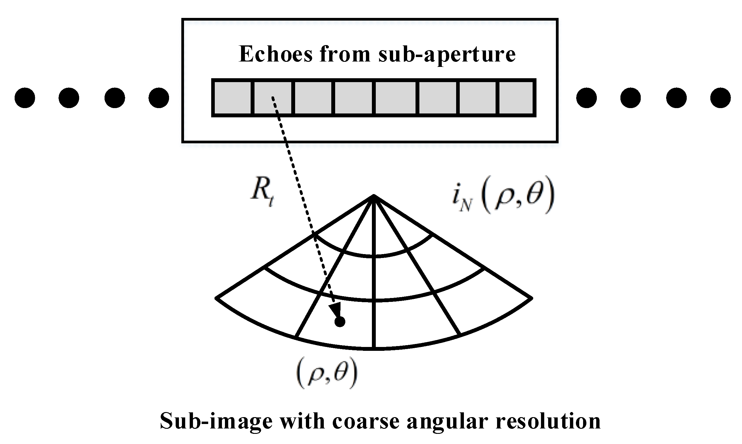
The implementation of FFBP algorithm contains two main stages. In the first stage, the full aperture is split into very small sub-apertures and the echoes from these small sub-apertures are projected onto polar grids by using direct BP algorithm. In this stage, only range history needs to be utilized for obtaining the coarse sub-image, as shown in Figure 1, and the angular history is not necessary. Let $i_N\left(\rho ,\theta \right)$ be the newly formed sub-image and $R_t$ be the range history from an arbitrary polar grid of $\left(\rho ,\theta \right)$ to the antenna phase centre (APC). In this stage, the range history of $R_t$ needs to be exactly calculated according to the geometry, based on which the echoes are processed onto the polar grid for obtaining $i_N\left(\rho ,\theta \right)$.

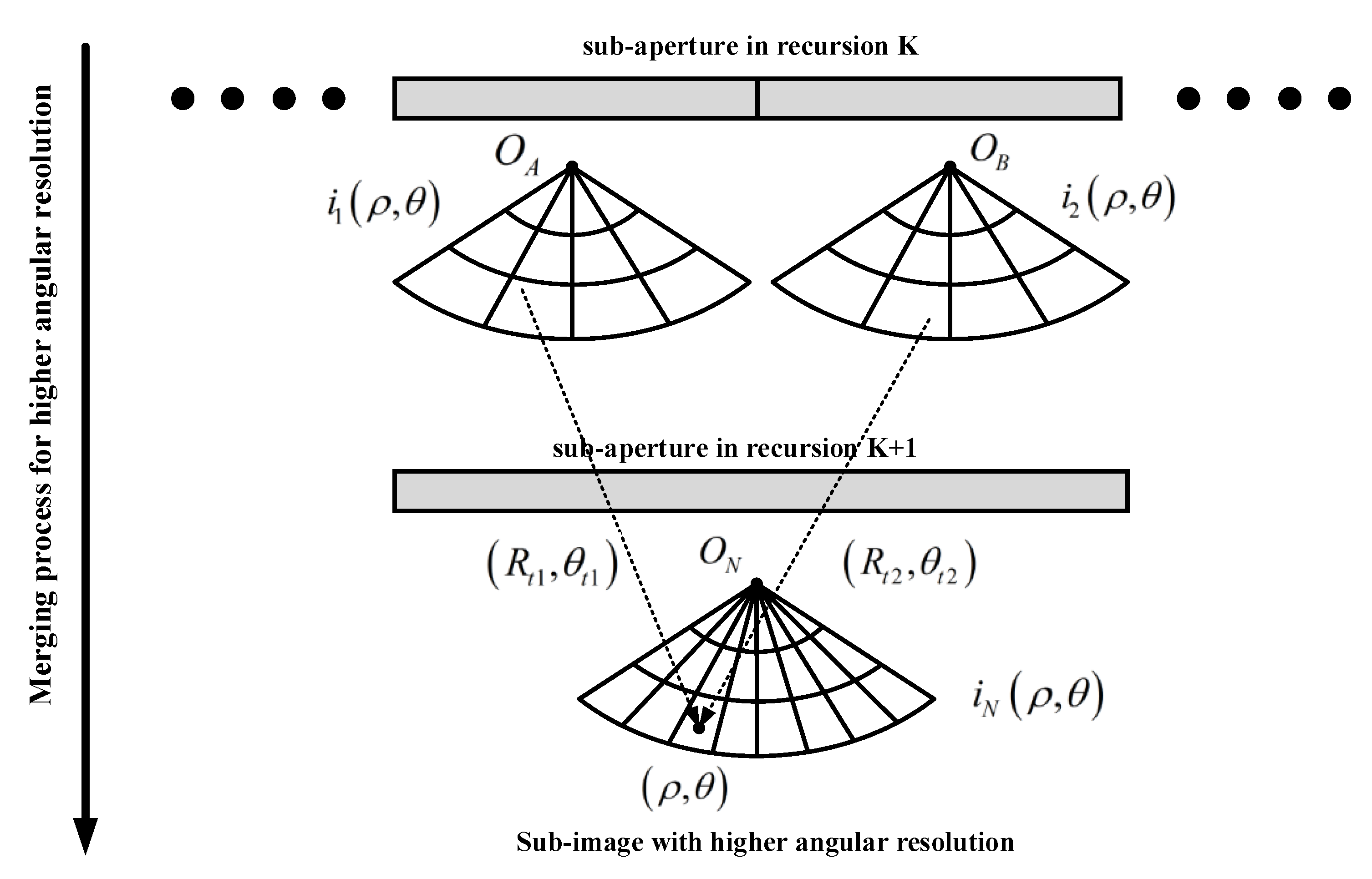
In the second stage of FFBP process, the sub-images are merged recursively to obtain higher resolution in angular direction. Figure 2 shows the merging process for a group of sub-images from recursion K to recursion K+1. Different from the operation in the first stage, in this stage, both range and angular histories need to be utilizing for mering process. Let $i_1\left(\rho ,\theta \right)$ and $i_2\left(\rho ,\theta \right)$ denote the sub-images in recursion K. $i_1\left(\rho ,\theta \right)$ is corresponding to the echoes from sub-aperture 1 while $i_2\left(\rho ,\theta \right)$ is corresponding to the echoes from sub-aperture 2. Let $i_N\left(\rho ,\theta \right)$ be the newly formed sub-image in recursion K+1. For an arbitrary grid of $\left(\rho ,\theta \right)$ in $i_N\left(\rho ,\theta \right)$, the range and angular histories in $i_1\left(\rho ,\theta \right)$ and $i_2\left(\rho ,\theta \right)$, denoted as $\left(R_{t1},{\theta }_{t1}\right)$ and $\left(R_{t2},{\theta }_{t2}\right)$, need to be exactly calculated according to the geometry, based on which the signal from $i_1\left(\rho ,\theta \right)$ and $i_2\left(\rho ,\theta \right)$ can be accordingly projected onto the newly formed $i_N\left(\rho ,\theta \right)$ with higher angular resolution. From the revisions above, it is can be noted that the accurate range and angular histories are the key point for obtaining high focusing performance in FFBP process. In the following section, the calculation for range and angular histories in missile-borne SAR focusing will be discussed carefully and the unknown tomography problem will be introduced.

3. The Tomography Problem in Missile-Borne SAR Focusing

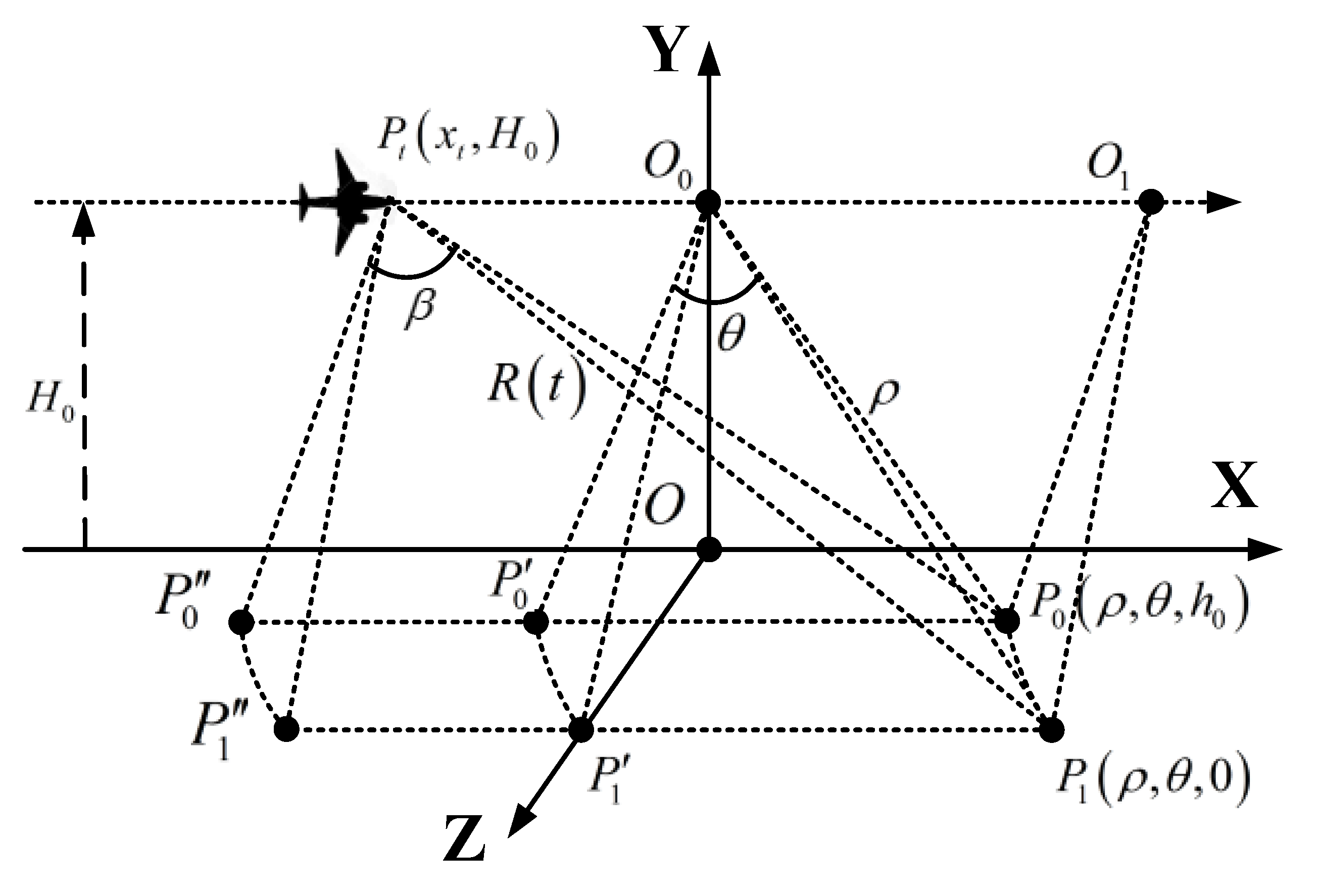
In this section, we compare the geometric acquisition of the FFBP process for both conventional airborne SAR and missile-borne SAR, then introduce the tomography problem in missile-borne SAR focusing with diving movement. First, we consider the airborne case. Figure 3 shows that the SAR sensor is mounted on an airplane and moving in a linear trajectory along the X direction. Let t denote the azimuth time. At t, the APC is at $P_t\left(x_t,H_0,0\right)$, where $H_0$ is the height of platform and $x_t$ can be regarded as a function of t as

$$\begin{array}{c}\hfill x_t=f_x\left(t\right).\end{array}$$

(1)

In the FFBP implementation, the echoed signal is processed on a polar grid to form a sub-image in every recursion [17]. Therefore, the algorithm development is based on the polar coordinate system. In the process, the range and the angular histories from APC to the arbitrary scatterer or grid need to be exactly calculated for the sub-image merging process in the FFBP implementation. Considering an arbitrary scatterer $P_0\left(\rho ,\theta ,h_0\right)$, where $\rho$ and $\theta$ are the coordinates in the polar coordinate system and $h_0$ is the tomography of the scatterer, as shown in Figure 3. $P_1\left(\rho ,\theta ,0\right)$ is another scatterer that has the same polar coordinates of $\rho$ and $\theta$ as $P_0$, but zero tomography. For $\rho$ and $\theta$, it has

$$\begin{array}{c}\hfill \left\{\begin{array}{c}\rho =\left|\overrightarrow{O_0{P}_0}\right|=\left|\overrightarrow{O_0{P}_1}\right|\hfill \\ \theta =\angle P_0^{\prime }{O}_0{P}_0=\angle P_1^{\prime }{O}_0{P}_1\hfill \end{array}\right..\end{array}$$

(2)

where $|·|$ denotes the length calculation for the range vector. In (2) and Figure 3, $P_0^{\prime }$, $P_1^{\prime }$, $P_0^{″}$, and $P_1^{″}$ denote the projections of $P_0$ and $P_1$ in different planes. The triangles $\Delta O_1{P}_0{P}_1$, $\Delta O_0{P}_0^{\prime }{P}_1^{\prime }$, and $\Delta P_t{P}_0^{″}{P}_1^{″}$ are parallel with each other, and all of these triangles are perpendicular to the X axis. With introduced projections of $P_0$ and $P_1$ in geometry, the range and the angular histories for $P_0$ with respect to the APC can be defined as

$$\begin{array}{c}\hfill \left\{\begin{array}{c}{R}_0\left(t\right)=\left|\overrightarrow{P_t{P}_0}\right|\hfill \\ {\beta }_0\left(t\right)=\angle P_0^{″}{P}_t{P}_0\hfill \end{array}\right..\end{array}$$

(3)

Similarly, the range and the angular histories for $P_1$ with respect to the APC can be defined as

$$\begin{array}{c}\hfill \left\{\begin{array}{c}{R}_1\left(t\right)=\left|\overrightarrow{P_t{P}_1}\right|\hfill \\ {\beta }_1\left(t\right)=\angle P_1^{″}{P}_t{P}_1\hfill \end{array}\right..\end{array}$$

(4)

In the FFBP implementation, the range and the angular histories for the scatterer or grid with respect to APC need to be exactly known for the sub-image merging process. Due to the cylindrical acquisition symmetry in the geometry, $P_0$ and $P_1$ have the same range and angular histories, given as

$$\begin{array}{c}\hfill \left\{\begin{array}{c}{R}_0\left(t\right)=R_1\left(t\right)=\sqrt{x_t^2+{\rho }^2-2\left|x_t\right|\rho cos\left(\frac{\pi }{2}+\theta \right)}\hfill \\ {\beta }_0\left(t\right)={\beta }_1\left(t\right)=arcsin\frac{\left|\overrightarrow{P_t{O}_1}\right|}{R_0\left(t\right)}\hfill \end{array}\right..\end{array}$$

(5)

Equation (5) reveals the fact that the range and the angular histories are independent to the target tomography. Only two coordinates of $\rho$ and $\theta$ are sufficient for calculating both the range and angular histories, and $P_0$ and $P_1$ will be focused on the same position in the final SAR image. Therefore, the focusing performance of the FFBP algorithm will not be much more sensitive to the scenario topography.

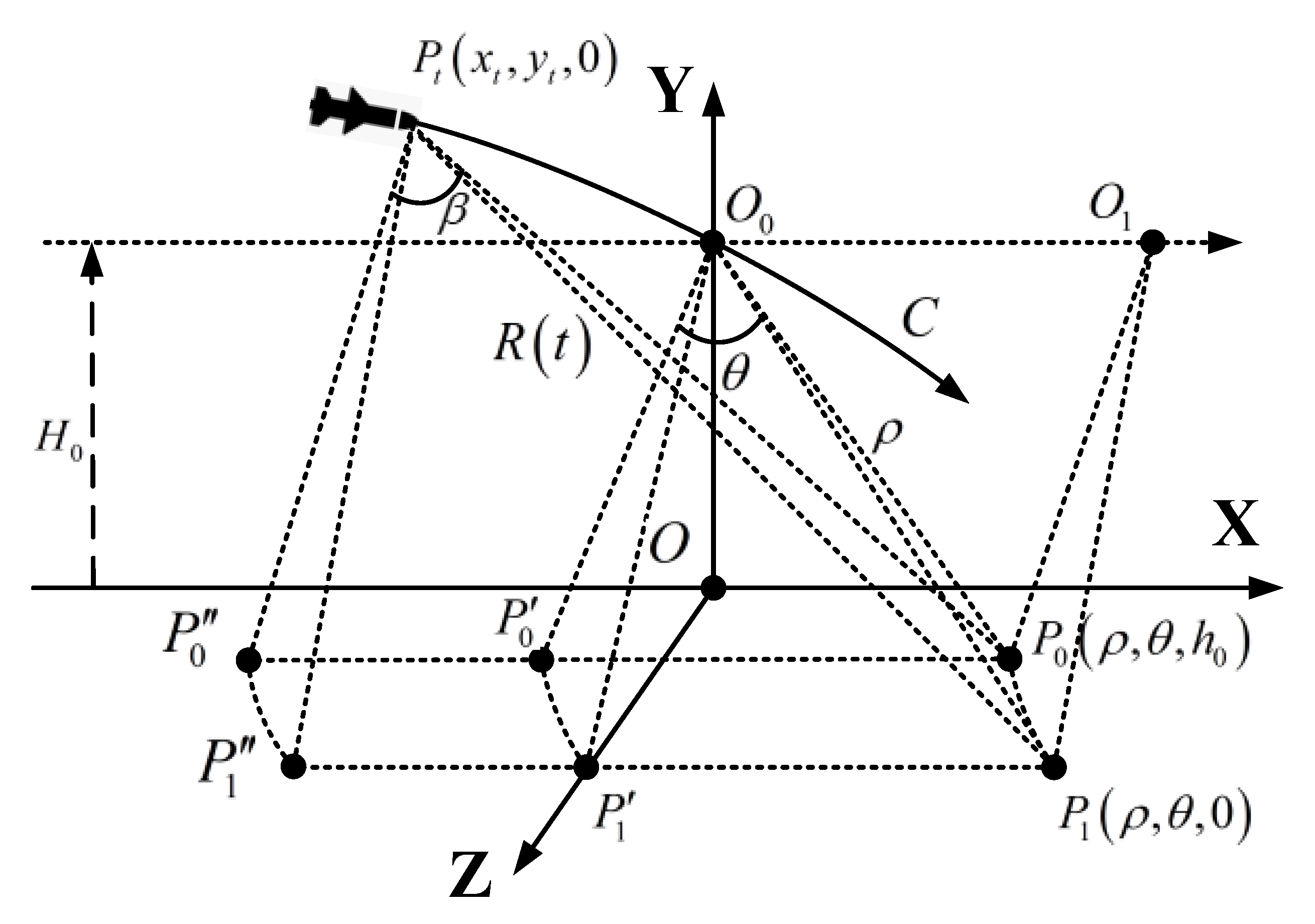
Then, we considered the case of missile-borne SAR with diving movement, as shown in Figure 4. In the operation, the SAR platform is moving along a diving curve trajectory of C. For simplicity, we assume the trajectory C is on $XOY$ plane. Let t denote the azimuth time. At t, the APC is at $\left(x_t,y_t,0\right)$, where $x_t$ and $y_t$ can be regarded as functions of t, as

$$\begin{array}{c}\hfill \left\{\begin{array}{c}{x}_t=f_x\left(t\right)\hfill \\ y_t=f_y\left(t\right)\hfill \end{array}\right..\end{array}$$

(6)

At $t=0$, the APC is at $\left(0,H_0,0\right)$. The positions of $P_0$ and $P_1$ as well as their coordinate definition are the same as the airborne case described in Figure 3 and (2). In Figure 4, $P_0^{\prime }$, $P_1^{\prime }$, $P_0^{″}$, and $P_1^{″}$ denote the projections of $P_0$ and $P_1$ in different planes. The triangles $\Delta O_1{P}_0{P}_1$, $\Delta O_0{P}_0^{\prime }{P}_1^{\prime }$, and $\Delta P_t{P}_0^{″}{P}_1^{″}$ are parallel with each other, and all of these triangles are perpendicular to the X axis. With introduced projections of $P_0$ and $P_1$ in the geometry, the range and angular histories for $P_0$ with respect to the APC can be defined as

$$\begin{array}{c}\hfill \left\{\begin{array}{c}{R}_0\left(t\right)=\left|\overrightarrow{P_t{P}_0}\right|\hfill \\ {\beta }_0\left(t\right)=\angle P_0^{″}{P}_t{P}_0\hfill \end{array}\right..\end{array}$$

(7)

Similarly, the range and angular histories for $P_1$ with respect to the APC can be defined as

$$\begin{array}{c}\hfill \left\{\begin{array}{c}{R}_1\left(t\right)=\left|\overrightarrow{P_t{P}_1}\right|\hfill \\ {\beta }_1\left(t\right)=\angle P_1^{″}{P}_t{P}_1\hfill \end{array}\right..\end{array}$$

(8)

According to the geometry, the range and angular histories for both $P_0$ and $P_1$ can be given by

$$\begin{array}{c}\hfill \left\{\begin{array}{c}{R}_0\left(t\right)=\sqrt{{\left(x_t-\rho sin\theta \right)}^2+{\left(y_t-h_0\right)}^2+\left[{\left({\rho }_{0}cos\theta \right)}^2-{\left(H_0-h_0\right)}^2\right]}\hfill \\ R_1\left(t\right)=\sqrt{{\left(x_t-\rho sin\theta \right)}^2+y_t^2+\left[{\left({\rho }_{0}cos\theta \right)}^2-H_0^2\right]}\hfill \\ {\beta }_0\left(t\right)=arcsin\frac{\left|\overrightarrow{P_0^{″}{P}_0}\right|}{R_0\left(t\right)}\hfill \\ {\beta }_1\left(t\right)=arcsin\frac{\left|\overrightarrow{P_1^{″}{P}_1}\right|}{R_1\left(t\right)}\hfill \end{array}\right..\end{array}$$

(9)

From (9), it can be seen that $P_0$ and $P_1$ have different ranges and angular histories. This reveals that the range and angular histories become sensitive to the scenario tomography in the missile-borne SAR case, which is quite different from the airborne SAR case. This is due to the fact that the acquisition symmetry of the circular cylindrical is no longer valid in the geometry with a diving curve trajectory. In the missile-borne SAR application with diving movement, the unknown tomography will inevitably introduce error in the range and angular calculations, which will seriously degrade the algorithm performance in focusing [23,24]. In the following section, a new algorithm was developed to address the tomography problem for achieving high focusing performance.

4. FFBP Algorithm Designed Based on Orthogonal Cylindrical Coordinate

To address the tomography problem in missile-borne SAR focusing, we introduced an orthogonal cylindrical coordinate (OCC) system, where the cross section of the cylindrical in the coordinate system is approximately orthogonal to the diving trajectory. The FFBP algorithm for missile-borne SAR focusing was designed based on the OCC system, and the implementation contains two main stages.

4.1. Stage 1

In the first stage of FFBP implementation, the full-aperture is divided into very small sub-apertures. The echo signal from the sub-aperture is then projected onto the local polar grid to obtain sub-images with low angular resolution. In this stage, only the range history needs to be utilized for forming coarse sub-images, and the range history is particularly investigated. In this stage of FFBP implementation, the OCC was designed according to the segmented trajectory corresponding to the small length of sub-aperture. Considering a small sub-aperture corresponding to a short segmented trajectory of $A{O}_{0}B$, where $O_0$ is the centre of the short segment, as shown in Figure 5. The straight line of L is the tangent of $A{O}_{0}B$ across $O_0$. The cylindrical coordinate system was designed according to the straight line of L, i.e., L is the axis of the cylinder. As the cross section of a cylinder in the coordinate system is approximately orthogonal to the trajectory, the newly designed cylindrical coordinate system is referred to as OCC system. So far, the OCC has been established and the process of the sub-aperture echoes are based on the OCC system for obtaining coarse sub-images.

Then, we considered two point scatterers with the same polar coordinates in the OCC system but different tomographies, denoted as $P_0\left(\rho ,\theta ,h_0\right)$ and $P_1\left(\rho ,\theta ,0\right)$, respectively, as shown in Figure 5. Note that, the coordinates of $\rho$ and $\theta$ defined in the OCC system are different from the airborne case described in Section 3. To describe the coordinates of $\rho$ and $\theta$, as well as the following range history, we introduce $P_0^{\prime }$, $P_1^{\prime }$, $P_0^{″}$, and $P_1^{″}$, which denote the projections of $P_0$ and $P_1$ in different planes. In Figure 5, the triangles $\Delta O_1{P}_0{P}_1$, $\Delta O_0{P}_0^{\prime }{P}_1^{\prime }$, and $\Delta P_t{P}_0^{″}{P}_1^{″}$ are parallel with each other, and all of these triangles are perpendicular to L. With introduced projections of $P_0$ and $P_1$ in the geometry, the coordinates of $\rho$ and $\theta$ for $P_0$ and $P_1$ in the OCC system can be given as

$$\begin{array}{c}\hfill \left\{\begin{array}{c}\rho =\left|\overrightarrow{O_0{P}_0}\right|=\left|\overrightarrow{O_0{P}_1}\right|\hfill \\ \theta =\angle P_0^{\prime }{O}_0{P}_0=\angle P_1^{\prime }{O}_0{P}_1\hfill \end{array}\right..\end{array}$$

(10)

The range history for $P_0$ with respect to the APC can be defined as

$$\begin{array}{c}\hfill \left\{\begin{array}{c}{R}_0\left(t\right)=\left|\overrightarrow{P_t{P}_0}\right|\hfill \\ {\beta }_0\left(t\right)=\angle P_0^{″}{P}_t{P}_0\hfill \end{array}\right..\end{array}$$

(11)

The range history for $P_1$ with respect to the APC can be defined as

$$\begin{array}{c}\hfill \left\{\begin{array}{c}{R}_1\left(t\right)=\left|\overrightarrow{P_t{P}_1}\right|\hfill \\ {\beta }_1\left(t\right)=\angle P_1^{″}{P}_t{P}_1\hfill \end{array}\right..\end{array}$$

(12)

In this stage of FFBP implementation, the segmented curve trajectory is generally designed with a very small length, e.g., four or eight azimuth samples, to achieve high computational efficiency. Therefore, the small length segment of the trajectory can be approximated as a straight line, and the geometric acquisition of OCC can be regarded as cylindrical symmetry. We assumed that at t, the APC is at $P_t$, as shown in Figure 5, and the range from $P_t$ to $O_0$ is denoted by $l_t$. Due to the acquisition symmetry of OCC system, $P_0$ and $P_1$ have nearly the same range history, given as

$$\begin{array}{c}\hfill R_0\left(t\right)\approx R_1\left(t\right)\approx \sqrt{l_t^2+{\rho }^2-2l_t\rho cos\left(\frac{\pi }{2}+\theta \right)}.\end{array}$$

(13)

From (13), the range history is nearly independent to the target tomography in the OCC system. While $P_0$ and $P_1$ have different tomographies, their range histories are only dependent on their polar coordinates of $\rho$ and $\theta$, which is quite different from the missile-borne SAR case of (9) described in Section 3. Therefore, in this stage of FFBP implementation, the coarse sub-images are formed in the designed OCC system and the calculation of the range history for the process is according to (13) to reduce the adverse affects of unknown tomography.

4.2. Stage 2

In the second stage of FFBP implementation, the coarse sub-images are merged recursively to achieve higher azimuthal resolution. The merging process for each group of sub-images in every recursion is also based on the designed OCC system to reduce the adverse affect of unknown tomography. The establishment of the OCC system in this stage is shown in Figure 6, which describes one group of sub-images for the merging process. We assume that sub-image 1 is corresponding to the sub-aperture of curve trajectory of $A{O}_0$ with the origin of $O_A$, while sub-image 2 is corresponding to the sub-aperture of curve trajectory of $O_{0}B$ with the origin of $O_B$. Both sub-image 1 and 2 are on their OCC system for forming a new image with higher angular resolution, and the new image is denoted as $i_N$. The newly formed $i_N$ corresponds to the long aperture of trajectory of $A{O}_{0}B$. Let the straight vector $\overrightarrow{O_A{O}_B}$ be the axis of the OCC system for $i_N$. Let $O_N$ denote the centre of $\overrightarrow{O_A{O}_B}$, and $O_N$ be the origin of $i_N$. So far, the OCC system for merging process has been established.

Then, we considered two scatterers with the same polar coordinates of $\rho$ and $\theta$ in the OCC but different tomographies, denoted as $P_0\left(\rho ,\theta ,h_0\right)$ and $P_1\left(\rho ,\theta ,0\right)$, respectively, as shown in Figure 6. Note that, different from the implementation in stage 1, in this stage, both the range and angular histories need to be utilized for the sub-image merging process. Here, we only investigated the merging process for sub-image 1. The merging process for sub-image 2 can be similarly investigated. To describe the coordinates of $\rho$ and $\theta$, as well as the range and angular histories, we introduce $P_0^{\prime }$, $P_1^{\prime }$, $P_0^{″}$, and $P_1^{″}$ which denote the projections of $P_0$ and $P_1$ in different planes. In Figure 5, the triangles $\Delta O_1{P}_0{P}_1$ and $\Delta O_N{P}_0^{\prime }{P}_1^{\prime }$ are parallel with each other, and both are perpendicular to L. Triangle $\Delta O_A{P}_0^{″}{P}_1^{″}$ is perpendicular to the straight vector $\overrightarrow{A{O}_0}$, but not exactly perpendicular to L. With introduced projections of $P_0$ and $P_1$ in the geometry, the coordinates of $\rho$ and $\theta$ for $P_0$ and $P_1$ in the OCC system can be given as

$$\begin{array}{c}\hfill \left\{\begin{array}{c}\rho =\left|\overrightarrow{O_N{P}_0}\right|=\left|\overrightarrow{O_N{P}_1}\right|\hfill \\ \theta =\angle P_0^{\prime }{O}_N{P}_0=\angle P_1^{\prime }{O}_N{P}_1\hfill \end{array}\right..\end{array}$$

(14)

The range and angular histories for $P_0$ with respect to sub-image 1 can be given as

$$\begin{array}{c}\hfill \left\{\begin{array}{c}{R}_0=\left|\overrightarrow{O_A{P}_0}\right|\hfill \\ {\beta }_0=\angle P_0^{″}{O}_A{P}_0\hfill \end{array}\right..\end{array}$$

(15)

Similarly, the range and angular histories for $P_1$ with respect to sub-image 1 can be given as

$$\begin{array}{c}\hfill \left\{\begin{array}{c}{R}_1=\left|\overrightarrow{O_A{P}_1}\right|\hfill \\ {\beta }_1=\angle P_1^{″}{O}_A{P}_1\hfill \end{array}\right..\end{array}$$

(16)

With the range and angular histories, sub-image 1 can be utilized for the merging process to form a new image. In the FFBP implementation, the focusing performance is more sensitive to the accuracy of the range history than that of the angular history in the merging process. Generally, the error of the range history needs to be less then one quarter of the wavelength for high focusing performance. Therefore, we first investigated the range history for the merging process. According to the geometry in the OCC system, $P_0$ and $P_1$ have the same range history with respect to the origin of $O_1$, given as

$$\begin{array}{c}\hfill R_0=R_1=\sqrt{|\overrightarrow{O_A{O}_N}{|}^2+{\rho }^2-2|\overrightarrow{O_A{O}_N}|\rho cos\left(\frac{\pi }{2}+\theta \right)}\end{array}$$

(17)

where $\left|\overrightarrow{O_A{O}_N}\right|$ is the length of the range vector $\overrightarrow{O_A{O}_N}$. From (17), the range history for the merging process is no longer dependent on the target tomography in the OCC system. While $P_0$ and $P_1$ have different tomographies, the range histories are only dependent to the polar coordinates of $\rho$ and $\theta$, which will dramatically reduce the adverse affects of the unknown tomography for achieving high focusing performance.

Then, we investigated the angular history of ${\beta }_0$ and ${\beta }_1$ with respect to $P_0$ and $P_1$ for the merging process. As shown in Figure 6, triangle $\Delta O_A{P}_0^{″}{P}_1^{″}$ is not exactly parallel to triangle $\Delta O_N{P}_0^{\prime }{P}_1^{\prime }$ due to the curve trajectory of the platform. Thus, ${\beta }_0$ is not exactly equal to ${\beta }_1$. In the FFBP process, the focusing performance is not so sensitive to the error of angular history as that of range history. Therefore the small difference between ${\beta }_0$ and ${\beta }_1$ will not bring serious degradation to the final focusing performance for most missile-borne SAR applications. We considered a set of typical parameters from a missile-borne SAR system, as shown in

Table 1. Parameters from a typical missile-borne SAR system.

Wave Band	Ku
Bandwidth	200 MHz
Height $H_0$	5000 m
Range Centre	about 10 km
Velocity in X Direction	600 m/s
Acceleration in X Direction	−20 m/$s^2$
Velocity in Y Direction	−150 m/s
Acceleration in Y Direction	−15 m/$s^2$
Synthetic Duration	0.8192 s

. The obtained resolution in both the range and azimuth directions was higher than 1 m, and 1m resolution is fine for most missile-borne SAR applications. The polar coordinates of $P_0$ and $P_1$ in the OCC system are given as $P_0\left(10,000\mathrm{m},\pi /3\mathrm{rad},100\mathrm{m}\right)$ and $P_1\left(10,000\mathrm{m},\pi /3\mathrm{rad},0\right)$, respectively. $P_0$ and $P_1$ have the same coordinates of $\rho$ and $\theta$, but different tomographies.

According to the geometry and parameters listed in Table 1, the angular value of ${\beta }_0$ for $P_0$ was $1.065227\mathrm{rads}$, while the angular value of ${\beta }_1$ for $P_1$ was $1.065263\mathrm{rads}$. In OCC-based FFBP algorithm, we introduce angular error of $\Delta \beta$ which denotes the difference between ${\beta }_0$ and ${\beta }_1$, which is dependent on the curvature of the trajectory as well as the tomography of the observing target. For FFBP process, $\Delta \beta$ needs to be smaller then the Nyquist sample in angular direction for achieving promising results, and the Nyquist sample is dependent on the designed azimuthal resolution. According to the geometry and SAR parameters, it can be calculated that the angular error of $\Delta \beta$ was approximately $3.57\times {10}^{-5}\mathrm{rads}$. We also calculated that the maximum Nyquist sample in the angular direction in the FFBP implementation [22] was $7.07\times {10}^{-5}\mathrm{rads}$, which is larger than the $\Delta \beta$. Therefore, the angular error of $\Delta \beta$ will not bring serious degradation to the focusing and the proposed OCC-based FFBP algorithm can dramatically reduce the adverse affects of unknown tomography in missile-borne SAR with diving movement. For missile-borne SAR focusing, the FFBP algorithm was designed according to the proposed OCC system to obtain high performance.

5. Simulation Experiments

In this section, simulation experiments based on a set of typical SAR parameters are presented and analyzed. The missile-borne SAR geometry for the simulation is given in Figure 7. The parameters are according to Table 1. In the simulation, we assumed that the illuminating scenario is a mountainous area of $800\mathrm{m}\times 800\mathrm{m}$ (X × Z directions) and nine point scatterers are considered in the SAR focusing. The nine point scatterers have different tomographies and their three dimensional coordinates are listed in

Table 2. The locations of the point scatterers.

Point	X	Y	Z
Point 1	4600 m	37.9 m	4600 m
Point 2	4600 m	23.2 m	5000 m
Point 3	4600 m	4.1 m	5400 m
Point 4	5000 m	16.1 m	4600 m
Point 5	5000 m	17.5 m	5000 m
Point 6	5000 m	−24.3 m	5400 m
Point 7	5400 m	3.3 m	4600 m
Point 8	5400 m	−6.1 m	5000 m
Point 9	5400 m	6.9 m	5400 m

.

The algorithms for the simulation experiments were programmed on a MATLAB platform and Windows 10 system on a desktop computer with an i7-9700 CPU and 32 GB RAM without parallel processing. The total processing time using direct BP was approximately 107 min. The total processing time using conventional FFBP was approximately 6.8 min. The total processing time using the proposed algorithm was approximately 6.9 min. The proposed algorithm had nearly the same computational burden as the conventional FFBP algorithm, both of which were much faster than the direct BP algorithm. In Figure 7, point 5 is regarded as the centre point while point 9 is regarded as the frontier point, both of which are particularly analyzed.

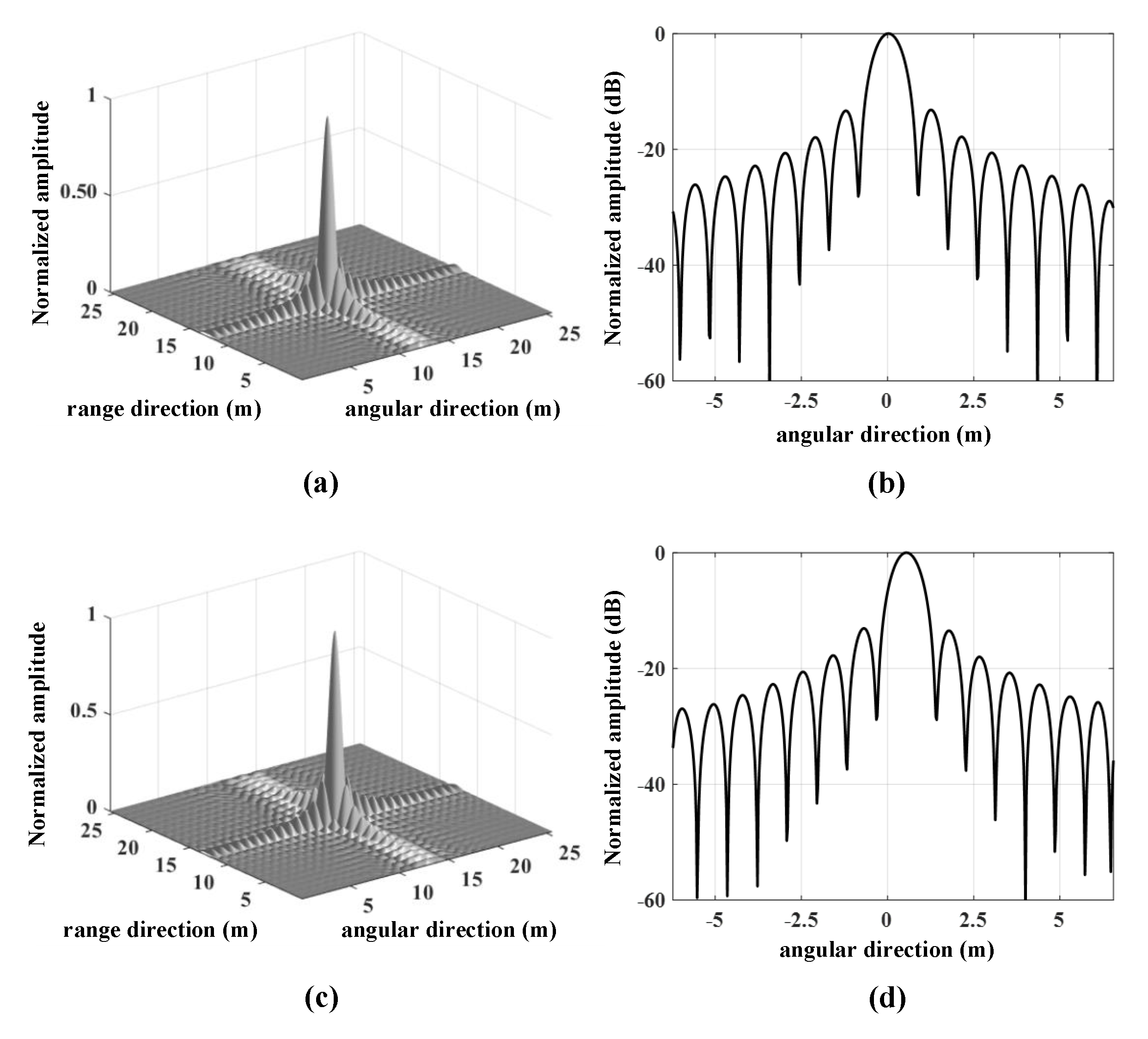
Figure 8 presents the focusing results of the centre point and frontier point obtained from the conventional FFBP algorithm. For the centre point, it can be calculated that the range and angular errors are 0.04 m and $1.75\times {10}^{-4}\mathrm{rads}$, respectively. For the frontier point, it can be calculated that the range and angular errors are 0.03 m and $1.34\times {10}^{-4}\mathrm{rads}$, respectively. The Nyquist sample in angular direction is $8.77\times {10}^{-5}\mathrm{rads}$. Due to the the unknown tomography information, the angular error far exceeds the Nyquist sample and will inevitably bring adverse affect in focusing. From Figure 8, it can be seen that the results degraded seriously along the azimuth direction due to the unknown tomography, and the defocusing results bring difficulty to the subsequent process. Figure 9 presents the focusing results of the centre point and frontier point obtained from the proposed OCC-based FFBP algorithm. For the centre point, it can be calculated that the range and angular errors in the OCC system are 0 m and $2.41\times {10}^{-5}\mathrm{rads}$, respectively. For the frontier point, it can be calculated that the range and angular errors in the OCC system are 0 m and $2.79\times {10}^{-5}\mathrm{rads}$, respectively. The Nyquist sample in angular direction is $7.07\times {10}^{-5}\mathrm{rads}$. It can be noted that the range errors have been completely removed and the angular errors are dramatically reduced. By comparing Figure 9 to Figure 8, it can be seen that the focusing performance of the proposed algorithm was superior to the conventional FFBP algorithm, where the processing result had a narrower main-lobe and lower sidelobes. The −3 dB main-lobe, the peak-sidelobe ratio (PSLR) and the integrated sidelobe ratio (ISLR) for the focusing quality analyses of the nine point scatterers are listed in

Table 3. The focusing quality of the point scatterers.

Range Direction
Point	3-dB width	PSLR	ISLR
Point 1	0.77 m	−12.92 dB	−9.91 dB
Point 2	0.78 m	−13.02 dB	−10.02 dB
Point 3	0.78 m	−12.96 dB	−9.97 dB
Point 4	0.77 m	−13.10 dB	−10.10 dB
Point 5	0.77 m	−13.15 dB	−10.11 dB
Point 6	0.78 m	−13.07 dB	−9.94 dB
Point 7	0.76 m	−12.87 dB	−9.89 dB
Point 8	0.77 m	−13.17 dB	−10.06 dB
Point 9	0.77 m	−13.05 dB	−10.03 dB
Angular direction
Point	3-dB width	PSLR	ISLR
Point 1	0.83 m	−12.81 dB	−9.84 dB
Point 2	0.86 m	−12.90 dB	−9.85 dB
Point 3	0.87 m	−12.78 dB	−9.79 dB
Point 4	0.85 m	−13.01 dB	−9.97 dB
Point 5	0.87 m	−13.01 dB	−9.92 dB
Point 6	0.88 m	−12.91 dB	−9.85 dB
Point 7	0.86 m	−12.91 dB	−9.94 dB
Point 8	0.89 m	−12.77 dB	−9.84 dB
Point 9	0.90 m	−13.08 dB	−10.01 dB

. The high focusing quality demonstrates the superior performance for missile-borne SAR focusing with diving movement.

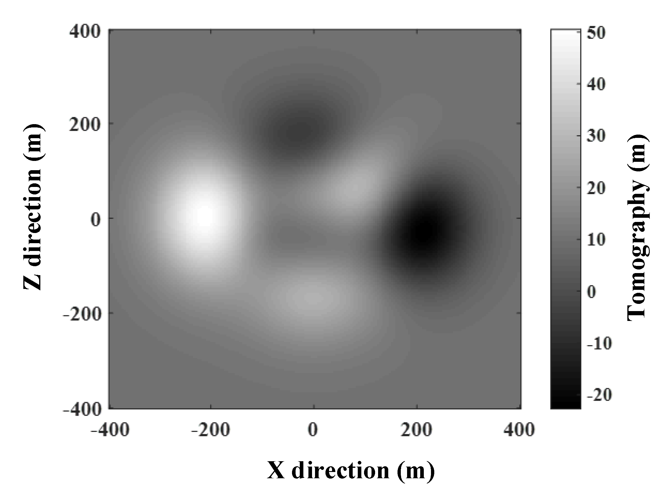
To further evaluate the performance of the proposed algorithm, a real scene simulation was implemented for both the conventional FFBP and the proposed algorithm. The simulation parameters were according to Table 1. The unknown tomography was also assumed and varied from 50 m to −20 m in a mountainous area of 800 m × 800 m (X × Z directions), as shown in Figure 10. The focusing results are provided in Figure 11. Figure 11a shows the results from the conventional FFBP algorithm, and the unknown tomography brings serious defocusing to the final image. Figure 11b shows the results from the proposed algorithm and shows that the proposed algorithm can effectively reduce the adverse affect of unknown tomography to achieve better performance that validates the superiority of the algorithm.

6. Discussion on the Limitation

In this section, we carefully discuss the limitation of the proposed algorithm. In FFBP process, both range and angular errors are significant for merging process. Based on the OCC geometry, the proposed algorithm can completely remove the range error. However, the angular error cannot be completely removed in the algorithm so that the defocusing may occur in some extreme cases. Even though, the proposed algorithm is meaningful because it can dramatically reduce the angular error for obtaining better focusing performance.

In the proposed OCC-based FFBP algorithm, there are two main factors to be considered for obtaining high performance focusing: The angular error as well as the Nyquist sample in angular direction. If the maximum of angular error is smaller than Nyquist sample, the angular error will not bring serious defocusing to the final image, otherwise, the defocusing is inevitable. The angular error is dependent on the curvature of the trajectory as well as the maximum tomography in the observing scenarios. Generally, the higher the curvature of the trajectory, the larger the angular error will be introduce. The larger the maximum tomography of the scenarios, the larger the angular error will be introduce. The angular error can be quantitatively estimated according to the geometry and SAR parameters. The Nyquist sample requirement in angular direction is dependent on the designed azimuthal resolution. In Section 5, the simulations are based on a set of typical parameters and the angular errors are smaller than Nyquist sample, thus the OCC-based FFBP obtained promising results.

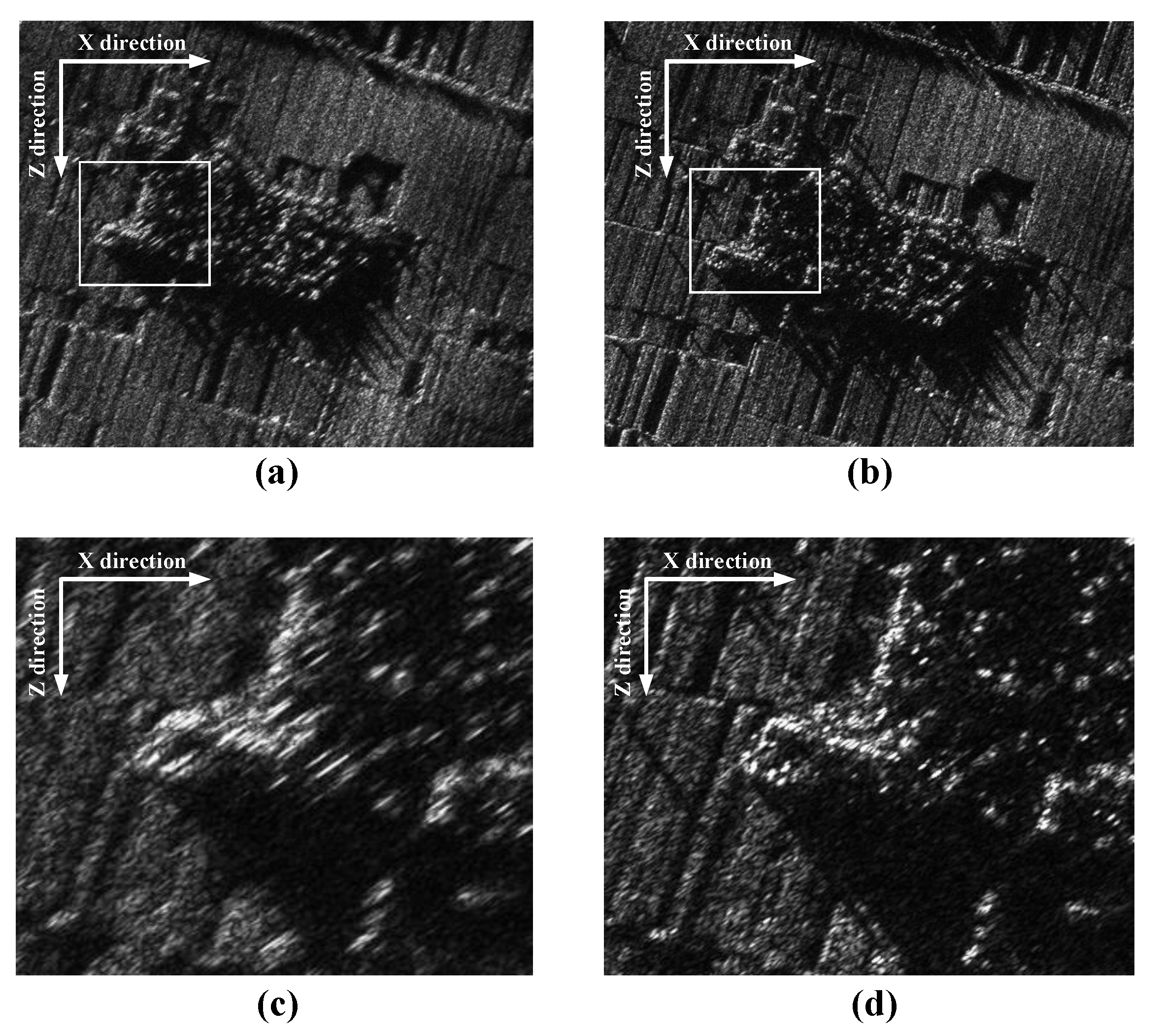
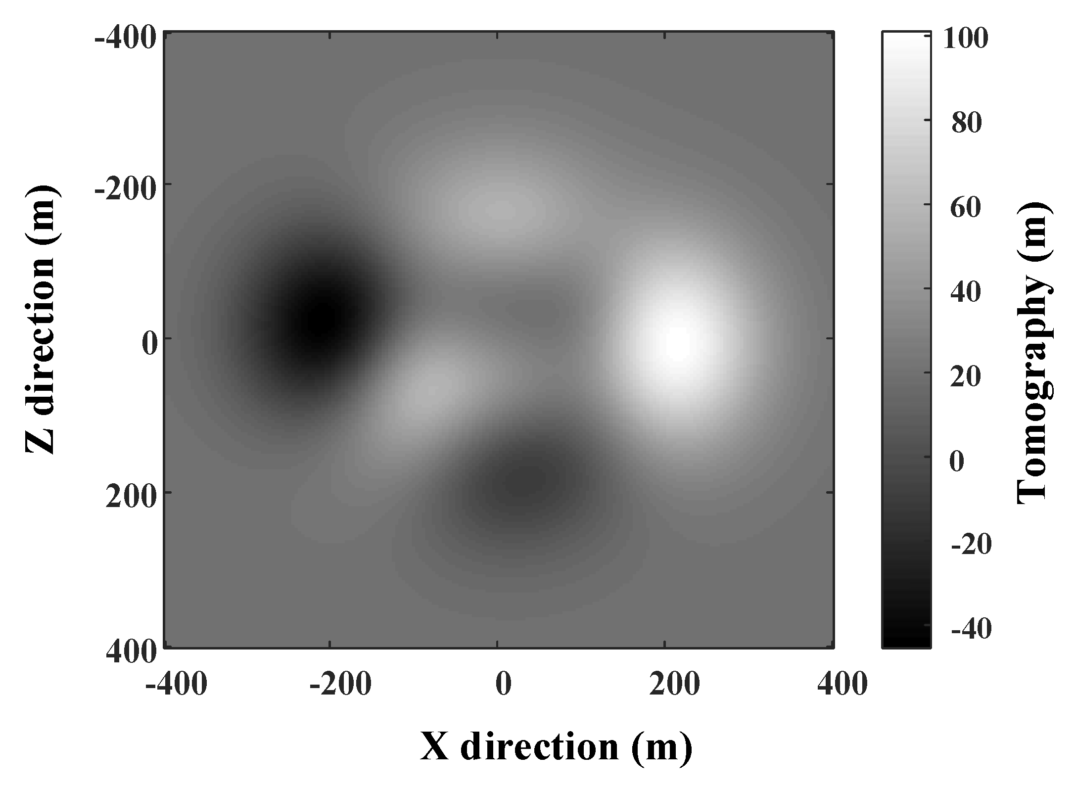
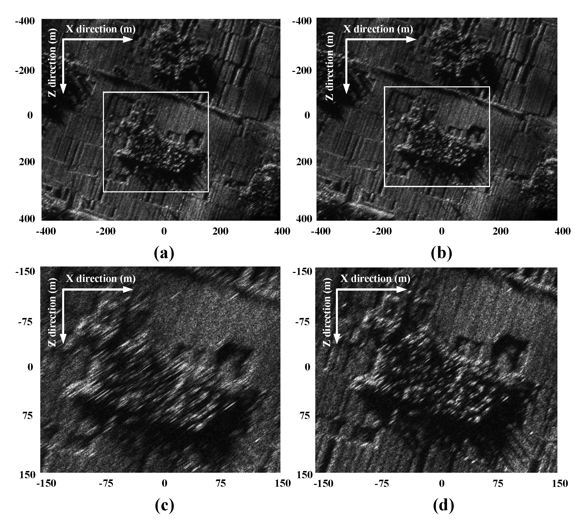
Then, we consider an extreme case of missile-borne SAR and the parameters are given in

Table 4. Parameters from an extreme case of a missile-borne SAR system.

Wave Band	Ku
Bandwidth	400 MHz
Height $H_0$	5000 m
Range Centre	about 10 km
Velocity in X Direction	600 m/s
Acceleration in X Direction	−40 m/$s^2$
Velocity in Y Direction	−150 m/s
Acceleration in Y Direction	−30 m/$s^2$
Synthetic Duration	1.6384 s

. The assumed tomography is varying from 100 m to −40 m, which is much more intense than the case simulated in Section 5, as shown in Figure 12. The geometry is the according to Figure 7. Comparing with the parameters in Table 1, the newly assumed trajectory has higher curvature, longer synthetic aperture duration as well as higher designed resolution (higher than 0.5 m). According to the geometry, the angular error in OCC system can be estimated, given as $6.87\times {10}^{-5}\mathrm{rads}$, and the Nyquist sample in angular direction is required to be smaller than $3.03\times {10}^{-5}\mathrm{rads}$. It can be seen that, the angular error exceeds Nyquist sample which will introduce defocusing to the final image. Figure 13a is the result from the conventional FFBP, and Figure 13b is the result from the proposed algorithm. Figure 13c,d are the zoomed images for comparison. While the proposed algorithm can obtain higher focusing performance comparing to the conventional FFBP, some defocusing is still in the result. To further improve the focusing quality, autofocusing technique can be developed with the OCC-based FFBP, which will be studied in our future work.

7. Conclusions

In this paper, the adverse effects of unknown tomography in missile-borne SAR focusing were carefully investigated, and a new FFBP algorithm was proposed to address the unknown tomography problem. The new algorithm was designed based on an orthogonal cylindrical coordinate (OCC) system. Owing to the advantages of the OCC system designed for the diving curve trajectory, the range history and angular histories of the grid became less dependent to the unknown tomography, which can dramatically reduce the topography sensibility to achieve high focusing performance. Simulation experiments were utilized to evaluate the proposed algorithm, and the experimental results showed that the algorithm can achieve higher focusing performance for general missile-borne SAR focusing with unknown tomography. The limitation of the proposed algorithm was also discussed. In future work, we will study efficient and effective autofocusing technique integrating with the OCC-based FFBP process which can further improve the focusing quality in missile-borne SAR applications.

References

- Moreira, A.; Prats-Iraola, P.; Younis, M.; Krieger, G.; Hajnsek, I.; Papathanassiou, K.P. A tutorial on synthetic aperture radar. IEEE Geosci. Remote Sens. Mag. 2013, 1, 6–43. [Google Scholar] [CrossRef] [Green Version]
- Buckreuss, S.; Schattler, B.; Fritz, T.; Mittermayer, J.; Kahle, R.; Maurer, E.; Boer, J.; Bachmann, M.; Mrowka, F.; Schwarz, E. Ten Years of TerraSAR-X Operations. Remote Sens. 2018, 6, 873. [Google Scholar] [CrossRef] [Green Version]
- Ezquerro, P.; Del Soldato, M.; Solari, L.; Tomás, R.; Raspini, F.; Ceccatelli, M.; Fernández-Merodo, J.A.; Casagli, N.; Herrera, G. Vulnerability Assessment of Buildings due to Land Subsidence Using InSAR Data in the Ancient Historical City of Pistoia (Italy). Sensors 2020, 20, 2749. [Google Scholar] [CrossRef]
- Wen, X.; Qiu, X. Research on Turning Motion Targets and Velocity Estimation in High Resolution Spaceborne SAR. Sensors 2020, 20, 2201. [Google Scholar] [CrossRef] [Green Version]
- Bie, B.; Sun, G.C.; Xia, X.G.; Xing, M.; Guo, L.; Bao, Z. High-speed maneuvering platforms squint beam-steering SAR imaging without subaperture. IEEE Trans. Geosci. Remote Sens. 2019, 57, 6974–6985. [Google Scholar] [CrossRef]
- Feng, D.; An, D.; Huang, X. An extended fast factorized back projection algorithm for missile-borne bistatic forward-looking SAR imaging. IEEE Trans. Aerosp. Electron. Syst. 2018, 54, 2724–2734. [Google Scholar] [CrossRef]
- Tang, S.; Guo, P.; Zhang, L.; Lin, C. Modeling and Precise Processing for Spaceborne Transmitter/Missile-Borne Receiver SAR Signals. Remote Sens. 2019, 11, 346. [Google Scholar] [CrossRef] [Green Version]
- Yuan, Y.; Chen, S.; Zhao, H. An Improved RD Algorithm for Maneuvering Bistatic Forward-Looking SAR Imaging with a Fixed Transmitter. Sensors 2017, 17, 1152. [Google Scholar] [CrossRef] [Green Version]
- Cumming, I.G.; Wong, F.H. Digital Signal Processing of Synthetic Aperture Radar Data: Algorithms and Implementation; Artech House: Norwood, MA, USA, 2004. [Google Scholar]
- Wu, J.; Sun, Z.; Li, Z.; Huang, Y.; Yang, J.; Liu, Z. Focusing Translational Variant Bistatic Forward-Looking SAR Using Keystone Transform and Extended Nonlinear Chirp Scaling. Remote Sens. 2016, 8, 840. [Google Scholar] [CrossRef] [Green Version]
- Rodriguez-Cassola, M.; Prats, P.; Krieger, G.; Moreira, A. Efficient time-domain image formation with precise topography accommodation for general bistatic SAR configurations. IEEE Trans. Aerosp. Electron. Syst. 2011, 47, 2949–2966. [Google Scholar] [CrossRef] [Green Version]
- Desai, M.D.; Jenkins, W.K. Convolution backprojection image reconstruction for spotlight mode synthetic aperture radar. IEEE Trans. Image Process. 1992, 1, 505–517. [Google Scholar] [CrossRef]
- Yang, L.; Zhou, S.; Zhao, L.; Xing, M. Coherent auto-calibration of APE and NsRCM under fast back-projection image formation for airborne SAR imaging in highly-squint angle. Remote Sens. 2018, 10, 321. [Google Scholar] [CrossRef] [Green Version]
- Lin, C.; Tang, S.; Zhang, L.; Guo, P. Focusing High-Resolution Airborne SAR with Topography Variations Using an Extended BPA Based on a Time/Frequency Rotation Principle. Remote Sens. 2018, 8, 1275. [Google Scholar] [CrossRef] [Green Version]
- Zhang, L.; Li, H.L.; Qiao, Z.J.; Xing, M.D.; Bao, Z. Integrating autofocus techniques with fast factorized back-projection for high-resolution spotlight SAR imaging. IEEE Geosci. Remote Sens. Lett. 2013, 10, 1394–1398. [Google Scholar] [CrossRef]
- Mao, X.; Ding, L.; Zhang, Y.; Zhan, R.; Li, S. Knowledge-Aided 2-D Autofocus for Spotlight SAR Filtered Backprojection Imagery. IEEE Trans. Geosci. Remote Sens. 2019, 57, 9041–9058. [Google Scholar] [CrossRef]
- Ulander, L.M.; Hellsten, H.; Stenstrom, G. Synthetic-aperture radar processing using fast factorized back-projection. IEEE Trans. Aerosp. Electron. Syst. 2003, 39, 760–776. [Google Scholar] [CrossRef] [Green Version]
- Zhou, S.; Yang, L.; Zhao, L.; Wang, Y.; Zhou, H.; Chen, L.; Xing, M. A New Fast Factorized Back Projection Algorithm for Bistatic Forward-Looking SAR Imaging Based on Orthogonal Elliptical Polar Coordinate. IEEE J. Sel. Top. Appl. Earth Obs. Remote Sens. 2019, 12, 1508–1520. [Google Scholar] [CrossRef]
- Pu, W.; Wu, J.; Huang, Y.; Yang, J.; Yang, H. Fast Factorized Backprojection Imaging Algorithm Integrated With Motion Trajectory Estimation for Bistatic Forward-Looking SAR. IEEE J. Sel. Top. Appl. Earth Obs. Remote Sens. 2019, 12, 3949–3965. [Google Scholar] [CrossRef]
- Bao, M.; Zhou, S.; Yang, L.; Xing, M.; Zhao, L. Data-driven Motion Compensation for Airborne Bistatic SAR Imagery under Fast Factorized Back Projection Framework. IEEE J. Sel. Top. Appl. Earth Obs. Remote Sens. 2020. [Google Scholar] [CrossRef]
- Ponce, O.; Prats-Iraola, P.; Scheiber, R.; Reigber, A.; Moreira, A. First airborne demonstration of holographic SAR tomography with fully polarimetric multicircular acquisitions at L-band. IEEE Trans. Geosci. Remote Sens. 2016, 54, 6170–6196. [Google Scholar] [CrossRef]
- Vu, V.T.; Pettersson, M.I. Nyquist sampling requirements for polar grids in bistatic time-domain algorithms. IEEE Trans. Signal Process. 2014, 63, 457–465. [Google Scholar] [CrossRef]
- Zhou, S.; Yang, L.; Zhao, L.; Bi, G. Quasi-polar-based FFBP algorithm for miniature UAV SAR imaging without navigational data. IEEE Trans. Geosci. Remote Sens. 2017, 55, 7053–7065. [Google Scholar] [CrossRef]
- Yang, L.; Li, P.; Zhang, S.; Zhao, L.; Zhou, S.; Xing, M. Cooperative Multitask Learning for Sparsity-Driven SAR Imagery and Nonsystematic Error Autocalibration. IEEE Trans. Geosci. Remote Sens. 2020, 58, 5132–5147. [Google Scholar] [CrossRef]
Figure 1.
Review of the first stage in the fast factorized back-projection (FFBP) process.
Figure 2.
Review of the second stage in the FFBP process.
Figure 3.
Airborne synthetic aperture radar (SAR) operating with a linear trajectory.
Figure 4.
SAR operated on a missile platform with a diving trajectory.
Figure 5.
Establishment of the orthogonal cylindrical coordinate (OCC) system in stage 1 of fast factorized back-projection (FFBP) implementation.
Figure 6.
Establishment of the orthogonal cylindrical coordinate (OCC) system in stage 2 of the FFBP implementation.
Figure 7.
The geometry for point target simulation in a mountainous area.
Figure 8.
The focusing results of the centre and frontier points from the conventional FFBP algorithm. The Nyquist sample in angular direction is . (a) Focusing results of the centre point, the range and angular errors are 0.04 m and , respectively. (b) Azimuth response of the centre point. (c) Focusing results of the frontier point, the range and angular errors are 0.03 m and , respectively. (d) Azimuth response of the frontier point.
Figure 9.
The focusing results of the centre and frontier points from the proposed algorithm. The Nyquist sample in angular direction is . (a) Focusing results of the centre point. (b) Azimuth response of the centre point, the range and angular errors are 0 m and , respectively. (c) Focusing results of the frontier point, the range and angular errors are 0 m and , respectively. (d) Azimuth response of the frontier point.
Figure 10.
The assumed tomography for a mountainous area in scene simulation.
Figure 11.
Focused SAR images of the scene simulation. (a) Obtained results from the conventional FFBP algorithm. (b) Obtained results from the proposed algorithm. (c) Zoomed image from the conventional FFBP. (d) Zoomed image from the proposed algorithm.
Figure 12.
The assumed tomography for a mountainous area in scene simulation in an extreme case.
Figure 13.
Focused SAR images of the scene simulation in the extreme case. (a) Results obtained from the conventional FFBP algorithm. (b) Results obtained from the proposed algorithm. (c) Zoomed image from the conventional FFBP. (d) Zoomed image from the proposed algorithm.