A Method to Detect and Track Moving Airplanes from a Satellite Video


1
Geospatial Information Sciences, The University of Texas at Dallas, 800 West Campbell Road, Richardson, TX 75080, USA
2
Key Laboratory of Digital Earth Science, Aerospace Information Research Institute, Chinese Academy of Sciences, Beijing 100094, China
3
Beijing Advanced Innovation Center for Imaging Technology, Capital Normal University, Beijing 100048, China
*
Author to whom correspondence should be addressed.
Remote Sens. 2020, 12(15), 2390; https://doi.org/10.3390/rs12152390
Submission received: 30 June 2020
/
Revised: 21 July 2020
/
Accepted: 23 July 2020
/
Published: 25 July 2020
(This article belongs to the Section Remote Sensing Image Processing)
Abstract
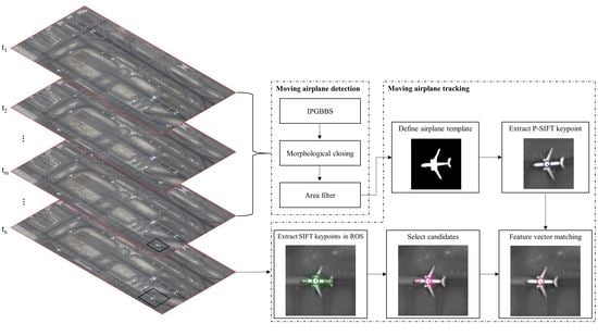
:In recent years, satellites capable of capturing videos have been developed and launched to provide high definition satellite videos that enable applications far beyond the capabilities of remotely sensed imagery. Moving object detection and moving object tracking are among the most essential and challenging tasks, but existing studies have mainly focused on vehicles. To accurately detect and then track more complex moving objects, specifically airplanes, we need to address the challenges posed by the new data. First, slow-moving airplanes may cause foreground aperture problem during detection. Second, various disturbances, especially parallax motion, may cause false detection. Third, airplanes may perform complex motions, which requires a rotation-invariant and scale-invariant tracking algorithm. To tackle these difficulties, we first develop an Improved Gaussian-based Background Subtractor (IPGBBS) algorithm for moving airplane detection. This algorithm adopts a novel strategy for background and foreground adaptation, which can effectively deal with the foreground aperture problem. Then, the detected moving airplanes are tracked by a Primary Scale Invariant Feature Transform (P-SIFT) keypoint matching algorithm. The P-SIFT keypoint of an airplane exhibits high distinctiveness and repeatability. More importantly, it provides a highly rotation-invariant and scale-invariant feature vector that can be used in the matching process to determine the new locations of the airplane in the frame sequence. The method was tested on a satellite video with eight moving airplanes. Compared with state-of-the-art algorithms, our IPGBBS algorithm achieved the best detection accuracy with the highest F1 score of 0.94 and also demonstrated its superiority on parallax motion suppression. The P-SIFT keypoint matching algorithm could successfully track seven out of the eight airplanes. Based on the tracking results, movement trajectories of the airplanes and their dynamic properties were also estimated.
1. Introduction
The advent of video satellites opens a new chapter in Earth observation [1,2,3,4,5,6,7]. These newly launched platforms can film videos of the Earth’s surface with sensors capable of “staring” at a specific area for several minutes’ duration. For example, the SkySat satellites can provide 30 frame-per-second (fps) panchromatic videos for up to 90 s with a spatial resolution of about 1 m. High definition satellite videos enable us to explore exciting applications far beyond the capabilities of remotely sensed imagery [1]. In a pioneer work by Kopsiaftis and Karantzalos [7], a SkySat satellite video was utilized to detect moving vehicles and estimate traffic density. In the 2016 Data Fusion Contest by the Image Analysis and Data Fusion Technical Committee of the IEEE Geoscience and Remote Sensing Society [3], satellite imagery and videos were used for activity analysis and traffic density estimation [6], change detection [8], global population modeling [9], etc.
However, the primary focus of satellite video-based studies has been on detecting and tracking moving objects. Yang et al. [5] used the saliency map derived from satellite video frames to detect moving vehicles and utilized their trajectories to generate a heat map for road network representation. Zhang et al. [4] detected moving vehicles with an emphasis on eliminating the false alarms caused by parallax motion in satellite videos. Ahmadi and Mohammadzadeh [10] tracked moving vehicles and vessels based on spatial proximity using the video captured from the International Space Station. Ahmadi et al. [2] used a SkySat video to estimate traffic parameters through the detection and tracking of moving vehicles. Shao et al. [1] developed a hybrid kernel correlation filter to track an individual moving object of middle to large size such as train, truck, and airplane in various satellite videos.
To date, the targets of moving object detection and tracking using satellite videos have been mostly vehicles, whereas moving airplanes have not been treated much in the literature. To the best of our knowledge, moving airplane tracking has been investigated in only few studies [1,11], which focused on tracking a single target. In addition to traffic monitoring, satellite videography may also provide practical values in supporting airport flow monitoring and scheduling, runway incursion warning, etc.
The challenges to detect and track moving vehicles and airplanes are very different. For moving vehicle detection, the main challenges are the low contrast of vehicles with the background [5] and mixed pixel problem. For moving vehicle tracking, the main challenge is the small size (2 × 2 pixels) of a vehicle that cannot provide stable features for tracking. Therefore, almost all existing studies use a tracking-by-detection strategy, which may not always yield satisfactory results. In contrast, the primary challenges for detecting moving airplanes are the foreground aperture problem caused by the long lengths of some slow-moving airplanes, as well as the false alarms introduced by the parallax motion of stationary airplanes. Compared with vehicles, airplanes are sufficiently large to provide stable features for accurate tracking, but how to achieve robust tracking, especially for rotating airplanes, remains a problem.
This objective of this paper is to develop a method to detect and track moving airplanes in an airport. First, we propose an Improved Gaussian-based Background Subtractor (IPGBBS) algorithm for moving airplane detection. This algorithm is able to effectively address the foreground aperture problem encountered by slow-moving airplanes in a satellite video. Second, detected moving airplanes are then tracked in the frame sequence through a Primary SIFT (P-SIFT) keypoint matching process, which incorporates the rotation invariance. This paper is organized as follows. Section 2 introduces the background research on moving object detection and moving object tracking. Section 3 describes the data and our method in detail. Section 4 provides the experimental results of the method applied to a satellite video with eight moving airplanes, followed by the discussion on computational efficiency and data availability in Section 5. Finally, Section 6 concludes this paper.
2. Background
In moving object detection studies, pixels for the moving objects are often referred to as the foreground, whereas pixels on stationary objects and unwanted moving objects (e.g., waving trees) are called the background. The detection of foreground pixels in each video frame is often achieved by subtracting background pixels [12]. Background subtraction creates a background model for each pixel, which defines a possible range(s) in which the background pixel’s values should reside. The simplest background model is the average or median of multiple video frames [2,7]. However, this simple model may not be able to handle various disturbances such as illumination change, movement of the camera, movement of the background. More sophisticated models have been developed in the computer vision field to detect moving objects in ordinary videos [13]. Chris and Grimson [14] proposed a more powerful Mixture of Gaussian (MoG) model to distinguish real foreground from moving background. This model, however, may produce incorrect detection if intensity changes abruptly. Kim et al. [15] built the background model as a codebook with K codewords. This model can handle abrupt changes of intensity but has high computation and memory requirements. Barnich and Droogenbroeck [16,17] proposed the Visual Background Extractor (ViBe) model, which creates a sample set for each background pixel, with the values in the sample set being randomly selected from the pixel’s history of values. This model can successfully detect moving objects at various speeds and perform accurate detection with camera motion, which is achieved by diffusing samples between neighboring pixel models. For this reason, ViBe was adopted to detect moving vehicles in a satellite video and achieved good detection accuracy [4,5].
In recent years, many deep learning approaches have been developed to detect moving objects in ordinary videos. These methods begin by detecting objects of interest with deep learning models [18,19,20,21]. Then, the dynamic status of each object is determined by the subsequent tracking procedure [22,23]. However, the process of object detection requires massive computation for the offline training process. Moreover, it is unclear if these approaches can successfully detect small-sized moving airplanes in satellite videos because limited by spatial resolution, such an airplane can be much smaller than the targets handled by these approaches.
For most tracking studies with ordinary videos, the strategy of tracking-by-detection has been widely adopted [24,25]. This strategy automatically links detected objects in the current frame to the nearest objects detected in the previous frame. Because of its simplicity, this approach has been widely adopted for tracking moving vehicles in satellite videos [2,5]. This approach highly relies on the accuracy and continuity of the preceding detection process because the identity of a detected vehicle can only be verified by spatial distance. If two different moving objects are close to each other in two consecutive frames, they may be mistakenly linked as the same object.
In contrast, the template matching technique can track moving objects in a more sophisticated way by verifying their spectral identity. Template matching starts with defining a template of a moving object from the previous frame, and then the template is moved (pixel-by-pixel) in the current frame to search for the most similar subset. To quantify the similarity between the template and each frame subset, the most straightforward measurements are pixel-wise correlations [26,27,28]. However, these measurements may fail to track objects with rotation due to their low rotation invariance [28,29]. To address this problem, image features of high rotation invariance can be compared as similarity measurements. Examples of image features are invariant moments [30,31], Zernike moments [32], orientation codes [33], ring-projection transformation [29,34]. Deep convolutional neural networks (CNNs) have also been used to track moving objects in ordinary videos through the effective extraction of deep features [35,36]. These deep features usually emphasize the generality of the objects rather than their differences, so the subsequent tracking may cause objects with a similar appearance to be mismatched. In addition, the limited spatial resolution of satellite video poses challenges for existing CNN approaches. As a result, traditional hand-crafted features are still favored for tracking multiple objects, especially those with similar appearances [37,38].
3. Materials and Methods
3.1. Satellite Video Data and Preprocessing
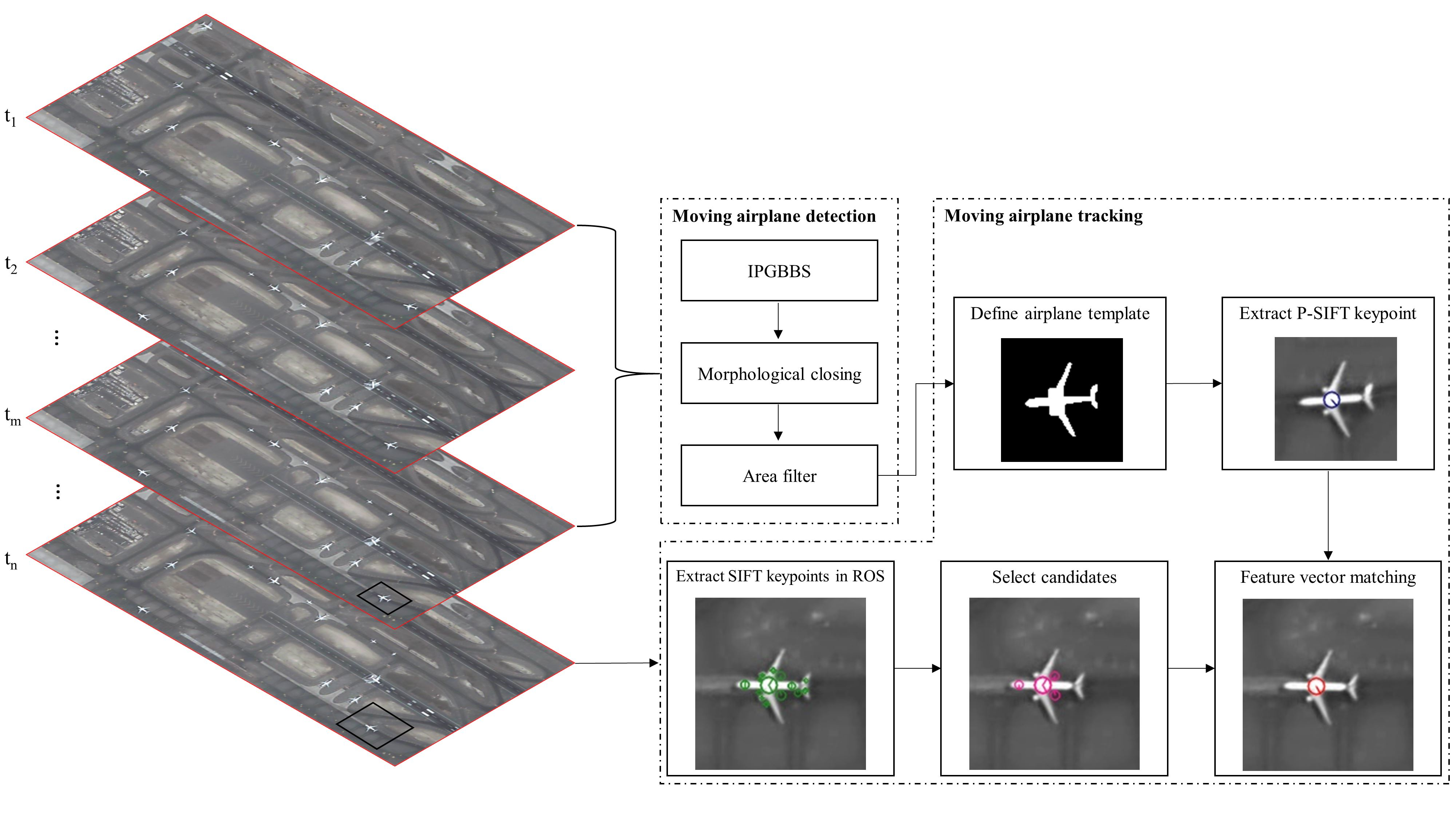
A true-color (RGB) high definition video acquired by a Jilin-1 satellite provided by Chang Guang Satellite Technology Co., Ltd. is used for this study. The original satellite video has a duration of 25 s with a frame rate of 10 fps, and a spatial resolution of 1 m. Since our targets of interest are moving airplanes, the original video is cropped to cover part of the Dubai International Airport between 25°15′50.90″N, 55°21′17.17″E and 25°14′52.11″N, 55°22′1.74″E (Figure 1a). Figure 1b,c shows the first and last frames of the cropped video with eight moving airplanes of various sizes. Among them, Airplane 1–6 are taxiing in a constant direction, whereas Airplane 7 and 8 are both taxiing and turning.
Preprocessing of the video data included frame sampling and greyscale conversion. All 250 video frames were split into a detecting sample set and a tracking sample set. The detecting sample set includes the first 150 frames (0–15 s), whereas the tracking sample set only includes the 170th, 190th, 210th, 230th, and 250th frames of the video in order to achieve a fast tracking. Frames in each sample set were converted into greyscale images by using:
where Fr, Fg and Fb denote pixel values of the red, green, and blue band, respectively.
3.2. Methods
3.2.1. Moving Airplane Detection by IPGBBS
Gaussian distribution was chosen as the background model to detect moving airplanes because it can be easily adapted to handle slight disturbances. In general, background subtraction has three components: model initialization, foreground/background classification, and model adaptation. Let I(x,y)0 denote the value of pixel (x,y) in the first detecting sample frame; the Gaussian background model for this pixel is initialized as:
Here, the pixel value is used as the initial mean of the Gaussian background model. The value of the standard deviation σ0 is assigned empirically according to the strength of disturbances. Specifically, if the satellite platform is moving very slowly relative to the ground, a small σ0 should be chosen. In a subsequent detecting sample frame t, the pixel (x,y) with its value denoted by I(x,y)t, can be classified as either background () or foreground () by:
where , respectively, represent the mean and standard deviation of the updated (or initialized) Gaussian background model in frame t−1, and is a predetermined threshold parameter. The larger is the value chosen for , the greater a pixel must deviate from the mean of the Gaussian distribution to be classified as foreground. Then, the parameters of the Gaussian background model are updated by:
where μt and σt denote the mean and standard deviation of the Gaussian background model at frame t. The learning rate α indicates the influence of frame t during the update and therefore controls how quickly the background model is being updated. In general, a low learning rate (low value for α) is suitable to detect slow objects, whereas a high learning rate (high value for α) is appropriate for detecting fast objects. In practice, the optimal value of α is obtained empirically.
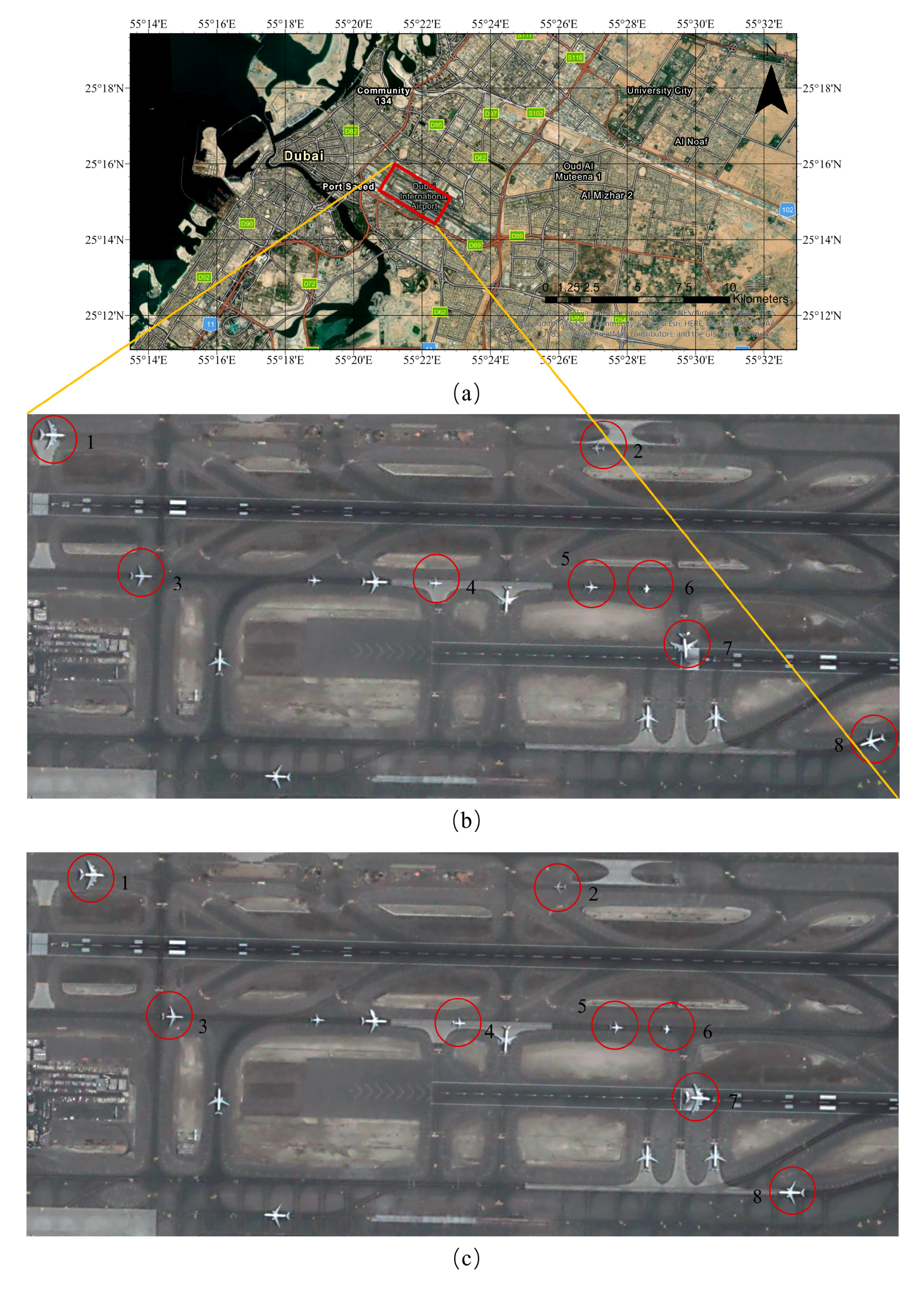
Conventionally, the adaption component uses one of two alternative strategies. One approach incorporates the value of I(x,y)t into the Gaussian background model regardless of its membership [7,10]. As shown in Figure 2a, this is equivalent to update both foreground and background with the same learning rate. This strategy may cause the underlying distribution to swing between background and foreground, although it is prone to the former. Consequently, some foreground pixels may be easily misclassified as background. The other approach incorporates the value of the incoming pixel into the Gaussian background model only if it belongs to the background. In this case, the Gaussian model at pixel (x,y) will not be updated if it belongs to the foreground. This strategy, however, may fail to adapt the background pixels initially occupied by the foreground [16,39]. Specifically, if pixel (x,y) belongs to the foreground in the first sample frame, its value is used to initialize the Gaussian background model. When pixel (x,y) in subsequent frames becomes the background, the Gaussian background model will continuously misclassify incoming background as foreground (false alarm in the white circle of Figure 2b).
In contrast, our algorithm, named Improved Gaussian Based Background Subtractor (IPGBBS), adopts a novel adaption strategy. Depending on the classification of the incoming pixel, model parameters for foreground and background pixels are adapted separately by different learning rates. Therefore, the value of learning rate α in Equation 4 is selected from the set {αf, αb}, representing the learning rate for the foreground and background, respectively. Figure 2c shows the detection result for the same airplane by using IPGBBS. Compared with traditional model adaptation strategies, the advantage of this novel strategy in IPGBBS is twofold. First, it is able to maintain a high accuracy of the Gaussian background model when pixel (x,y) belongs to the foreground. Second, it is able to gradually adapt the Gaussian background model for a pixel initially occupied by a moving object so that the Gaussian background model will represent the real background.
The fragmented detection in Figure 2a also indicates that the traditional approach suffers from the foreground aperture problem with a slow-moving object. In this case, some locations may be continuously covered by the similar foreground pixels in may frames. Pixels on these locations may be easily misclassified as background because the change of pixel values is so small. As a result, the moving object detected may be incomplete or include small holes and gaps. In contrast, IPGBBS can alleviate this problem by the simultaneous use of a fairly low background learning rate and an even lower foreground learning rate. In addition to the slow speed, the foreground aperture problem can also be caused by a high degree of spectral homogeneity of the airplane [40,41], which leads to the airplane’s tail separated from the main body in Figure 2c. To further deal with this problem, a morphological closing operation is applied to the preliminary detection. The morphological closing operation consists of dilation and erosion. The dilation first fills small holes and gaps, and then the erosion recovers the real boundary of the foreground. Figure 2d demonstrates the result of the morphological closing, wherein the previously separated main body and tail are successfully connected. Additionally, the detected foreground may contain noise and false alarms caused by local spectral variation and camera jitter. These noise and false alarms are usually small, thus can be easily rejected by an area filter with a threshold parameter ρ. If an object’s area is smaller than ρ, the object is labeled as background, and excluded from the subsequent tracking process.
3.2.2. SIFT Based Keypoint and Feature Vector Extraction
Our moving airplane tracking algorithm follows a keypoint matching paradigm, in which keypoints of moving airplanes detected in the previous frame are used to match those in the subsequent frames. Various keypoints generation algorithms, including SURF, SIFT, and PCA-SIFT, were compared, and SIFT was adopted because of the highest rotation and scale invariance of the SIFT feature vector [42].
To extract SIFT keypoints from image ℓ, we start with building its scale-space, L, by convolving image ℓ with a variable-scale Gaussian function G(x,y,η):
where represents a convolution operation and η the scale variable. This process is commonly referred to as a Gaussian smoothing, where a larger η means a higher level of smoothing. To establish a continuous scale space of image ℓ, variable η is incrementally multiplied by a factor k. Meanwhile, image ℓ is down-sampled (halved) after each n times of Gaussian smoothing operation. As a result, image ℓ is incrementally smoothed and down-sampled to construct its scale space as a pyramid of N octaves (each octave represents one down-sampling). In each octave, the Difference of Gaussian (DOG) images are obtained by differencing adjacent smoothed images in the same octave as:
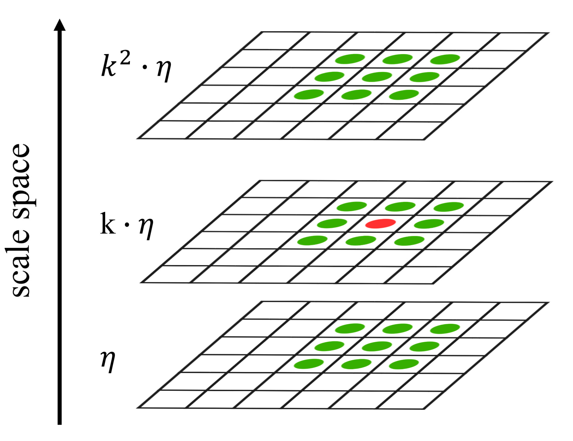
Subsequently, scale-space extrema are identified by comparing each pixel (red pixel in Figure 3) in a DOG with its neighbors in the current DOG and the DOGs above and below (green pixels in Figure 3). These extrema are further filtered to reject those with low contrast (low distinctiveness) or strong edge response (low repeatability) before they are eventually determined as SIFT keypoints.
For each SIFT keypoint, its basic properties can be represented by a vector as:
where (x,y) represents the keypoint’s location in ℓ, H represents the scale variable from which the SIFT keypoint is extracted, and Θ represents the dominant gradient extracted from the neighborhood of pixel (x,y). Based on , a SIFT keypoint can be represented in ℓ as a circle (Figure 4), where (x,y) denotes the center of the circle, H is the radius length, and Θ is the angle of a specific radius.
In addition to , gradient orientations from the neighborhood of pixel (x,y) are summarized to form a feature vector for the SIFT keypoint. The keypoint is extracted from the continuous scale space of the image, and the extracted feature vector is able to achieve scale invariant. According to Lowe’s algorithm [43], the coordinates of the neighborhood and the gradient orientations inside the neighborhood are rotated according to Θ in order to achieve rotation invariance. The neighborhood is further divided into multiple subregions. Then, in each subregion, the gradient orientations of pixels are grouped into eight directions, representing eight bins in a gradient histogram. The length of each bin is represented by the accumulated gradient magnitudes of the corresponding pixels. Originally, the feature vector is extracted from four by four subregions with each subregion 4 × 4 pixels in size. However, considering the general size of an airplane in a remotely sensed video frame, we decided to use two by two subregions but kept each subregion at 4 × 4 pixels in size.
3.2.3. Moving Airplane Tracking by P-SIFT Keypoint Matching
Since our IPGBBS algorithm utilizes a recursive model, more accurate detection is expected in later frames. Therefore, only the result from the last detecting sample frame, denoted by F0, is used as input to the subsequent tracking algorithm. Our tracking algorithm starts with defining templates from F0 based on the estimated bounding box of each moving airplane. To guarantee a sufficiently large neighborhood for feature vector extraction, the size of each template is extended by a predefined value of δtemp. However, the enlarged template may include some SIFT keypoints outside the airplane. Therefore, a screening process is conducted by using the detected area as a mask. The resulting SIFT keypoints on a detected moving airplane are identified as:
Conventionally, matching keypoints in different frames requires adequate and repeatable keypoints. Otherwise, keypoints in a frame may easily be mismatched to wrong keypoints in another frame, leading to an incorrect tracking. Moving objects tracked in ordinary videos may easily fulfill these prerequisites due to their large sizes and high spectral heterogeneity. In contrast, moving airplanes in satellite videos are often relatively small and homogeneous, and therefore may not have adequate and repeatable keypoints for tracking. For example, many of the keypoints on the “large” airplane shown in Figure 4 have very low repeatability because of its low spectral heterogeneity. Using such SIFT keypoints could easily mislead the tracking of the moving airplane.
Fortunately, at least one keypoint of an airplane demonstrates the highest repeatability among all the SIFT keypoints. We name this keypoint as the Primary SIFT (P-SIFT) keypoint of the airplane, denoted by . Figure 4 suggests that the airplane’s P-SIFT keypoint is always represented by the largest circle located at the center of the airplane because it is identified in the highest scale space. During the process of SIFT keypoint extraction, the whole airplane is incrementally smoothed and down sampled. SIFT keypoints along edges are first identified because they are immediately connected with the background. As the scale-space becomes higher, the airplane is increasingly shrunk towards a single pixel. When this pixel finally meets the background, it becomes a local extremum. After investigating all the airplanes in different video frames, we found the following distinct properties of their P-SIFT keypoints:
- High distinctiveness: The P-SIFT keypoint has the largest scale variable among all SIFT keypoint of the same airplane.
- High repeatability: For an airplane having a spectral contrast with its surrounding background, its P-SIFT keypoint can always be detected in any video frame.
- High stability of the feature vector: For an airplane with consistent spectral properties, the feature vector of its P-SIFT keypoint is highly rotation and scale invariant in the frame sequence.
Based on the high distinctiveness property, the P-SIFT of a moving airplane can be found from CT by:
where is the P-SIFT keypoint of the moving airplane in the template, and it has the largest η among all SIFT keypoints. Figure 5 shows the P-SIFT keypoint of the moving airplane extracted from the frames in Figure 4. The same P-SIFT keypoint has been successfully identified in all frames, which validates its high repeatability. More importantly, the P-SIFT has a feature vector of the highest stability among all SIFT keypoints because the P-SIFT keypoint is located near the center of the airplane surrounded by its neighboring pixels from the same airplane. The high stability property of its feature vector makes the P-SIFT ideal for the keypoint matching process. Therefore, our algorithm only uses the P-SIFT keypoint for matching to achieve moving airplane tracking, that is, we search for the SIFT keypoints corresponding to in tracking sample frames.
Given the data volume of a satellite video frame, it can be computationally expensive to extract SIFT keypoints and their feature vectors from the whole frame. Therefore, SIFT keypoint matching is conducted only in a region of search (ROS) of each moving airplane in a tracking sample frame. The ROS of an airplane can be defined by its upper left coordinates ULros and lower right coordinates LRros as:
where shift is the translation estimated by the previous tracking of the same airplane and δros is a predefined parameter to control the size of the ROS, which should be larger than the template. Let set Cros denote all SIFT keypoints detected from the ROS; it is possible that some SIFT keypoints in Cros are located outside the airplane. To find the correct SIFT keypoint corresponding to , an intuitive approach is to match all SIFT keypoints of Cros with . However, our tracking algorithm adopts a more efficient two-scan procedure to enhance tracking efficiency. In the first scan, a set Ccandi of M candidate keypoints is selected from Cros by:
where function sorted rearranges all SIFT keypoints in Cros based on the descending order of their scale variable. Theoretically, the scale variable of an airplane’s P-SIFT keypoint is positively related to the size, thus a larger airplane should have a larger scale variable for its P-SIFT keypoint than a smaller one. If the ROS includes multiple objects (with the number of objects less than M), the above equation extracts the P-SIFT keypoints of all objects in the ROS, and the target airplane should be one of them. In the second scan, candidates in Ccandi are individually matched with based on the feature vector similarity. Consequently, the P-SIFT keypoint of the tracked moving airplane in the ROS, denoted by , is retrieved by:
where is the feature vector of , is the feature vector of the mth keypoint in Ccandi, and q is the dimensions of the feature vector. If a keypoint in Ccandi has the highest similarity with among all the keypoints in Ccandi, this keypoint is determined as the P-SITF keypoint of the moving airplane in ROS. Consequently, the location of the keypoint is designated as the tracked location of the moving airplane in the current tracking sample frame.
3.3. Accuracy Assessment
We use recall, precision, and F1 score to assess the performance of the developed IPGBBS moving airplane detection algorithm at the object level. Given the number of detected objects being true positive (TP), false positive (FP), and false negative (FN), these metrics are defined as:
It is worth noting that a moving airplane may be detected as several parts, but only one of them is treated as TP, while others are considered as FPs. The accuracy of the developed moving airplane tracking algorithm is also assessed at the object level by the visual verification of whether the tracked locations are on the same moving airplane or not.
4. Results
4.1. Results of Moving Airplane Detection
The performance of the IPGBBS algorithm was compared with three state-of-the-art algorithms: Codebook [15], Mixture of Gaussians (MoG) [14], and Visual Background Extractor (ViBe) [16,17]. These algorithms have been widely used in computer vision for detecting moving objects in ordinary videos, but only ViBe has been applied to satellite videos for moving vehicle detection [4,5]. Parameters used for the three comparison algorithms were estimated based on the best results in different trails. Table 1 displays the parameters of IPGBBS obtained based on empirical trails. Initial results by four algorithms (Codebook, ViBe, MoG, and IPGBBS) were further boosted with a morphological closing and area filter, with the minimum area ρ being set to 60 pixels, which should be smaller than the smallest airplane while larger than the general sizes of false alarms.
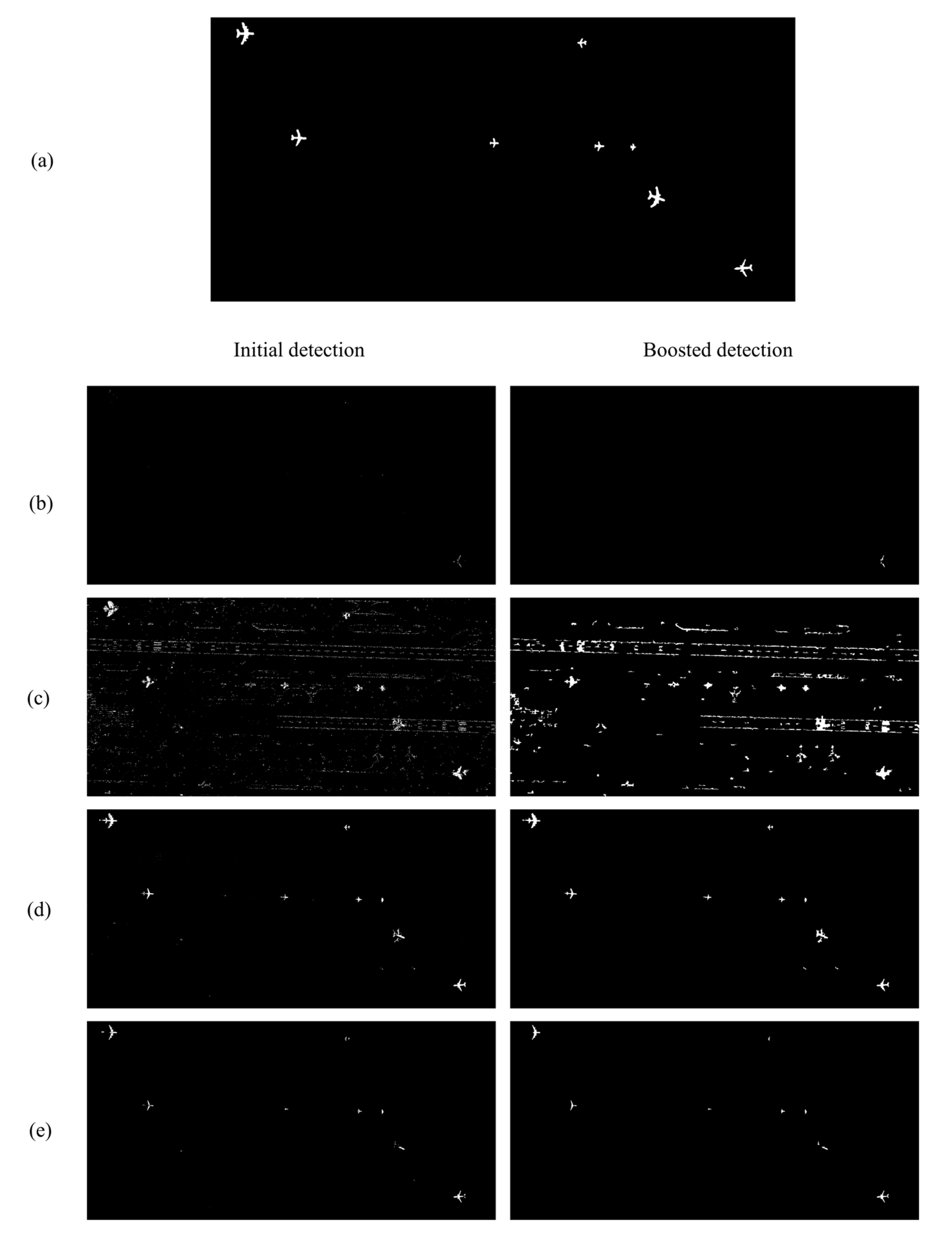
The performance of initial detection and boosted detection are shown in Figure 6, and the accuracy assessment is given in Table 2. Codebook can only detect the fastest airplane (Airplane 8) in both the initial and the boosted detection results. This indicates that Codebook possesses low sensitivity to slow-moving airplanes, leading to the lowest recall among all algorithms. From the incomplete detection of the only airplane, we can see that Codebook is also greatly affected by the foreground aperture problem. The initial detection by MoG includes many FPs caused by the movement of the remote sensing platform. Most FPs have sizes larger than ρ (60 pixels), and therefore cannot be removed by the area filter. As a result, MoG has the lowest precision and F1 score among all methods. The ViBe has a recall of 1 because it successfully detects all moving airplanes. However, it has a lower precision compared to our algorithm since it detects more FPs. In both the initial detection and boosted detection results, ViBe has better performance than Codebook and MoG, but poorer performance than our algorithm. In addition, the performance of both MoG and ViBe has been degraded by parallax motion. For example, ViBe produces two FPs between Airplane 7 and 8 in the boosted detection. In the original video, two stationary airplanes are parking at this location, and their parallax motion results in the reduced precision of ViBe. Overall, our method has the highest possible recall of 1 and the highest precision among all methods, leading to the highest F1 score of 0.942 for the boosted detection result. This result indicates that our IPGBBS algorithm is able to detect all the moving airplanes with the lease number of FPs (only 1).
Based on Figure 6 and Table 2, it is clear that the morphological closing and area filter have greatly enhanced the performance of all algorithms, especially on FP suppression. For example, our algorithm includes 34 FPs in the initial detection result, and this number reduces to 1 in the boosted detection result. Additionally, the foreground aperture problem has been effectively suppressed by using morphological closing. However, the foreground aperture problem is still observed for multiple moving airplanes. The missing parts are mainly from the rear half of fuselages, where the foreground aperture problem has an even greater effect than other parts. The moving Airplane 7 is initially detected as multiple parts by MoG, ViBe, and IPGBBS, whereas Codebook does not even detect it. This airplane is moving over a zebra crossing (crosswalk with alternating black and white stripes) where the white lines have similar intensities to the airplane. These algorithms cannot detect the portions of the airplane superimposed on the white lines because of the so-called camouflage problem [40]. Even though our IPGBBS algorithm overall has the highest accuracy at the object level, it cannot detect this airplane as an integral whole under these circumstances. A possible solution to the camouflage problem is to use a relatively lower threshold φ with IPGBBS, which however may introduce more FPs into the detection result, and therefore was not adopted.
4.2. Results of Moving Airplane Tracking
In the moving airplane tracking stage, the detection result from the boosted IPGBBS detection (Figure 6e) is used to define templates for the eight moving airplanes. Their locations in each tracking sample frame are retrieved by using the developed P-SIFT keypoint matching algorithm. The values of δtemp and δros were set at 20 and 40, respectively; the scale variable η for Gaussian smoothing was set at 2; factor k was set at , as suggested in [43]; and the number of candidates M was set at 5.
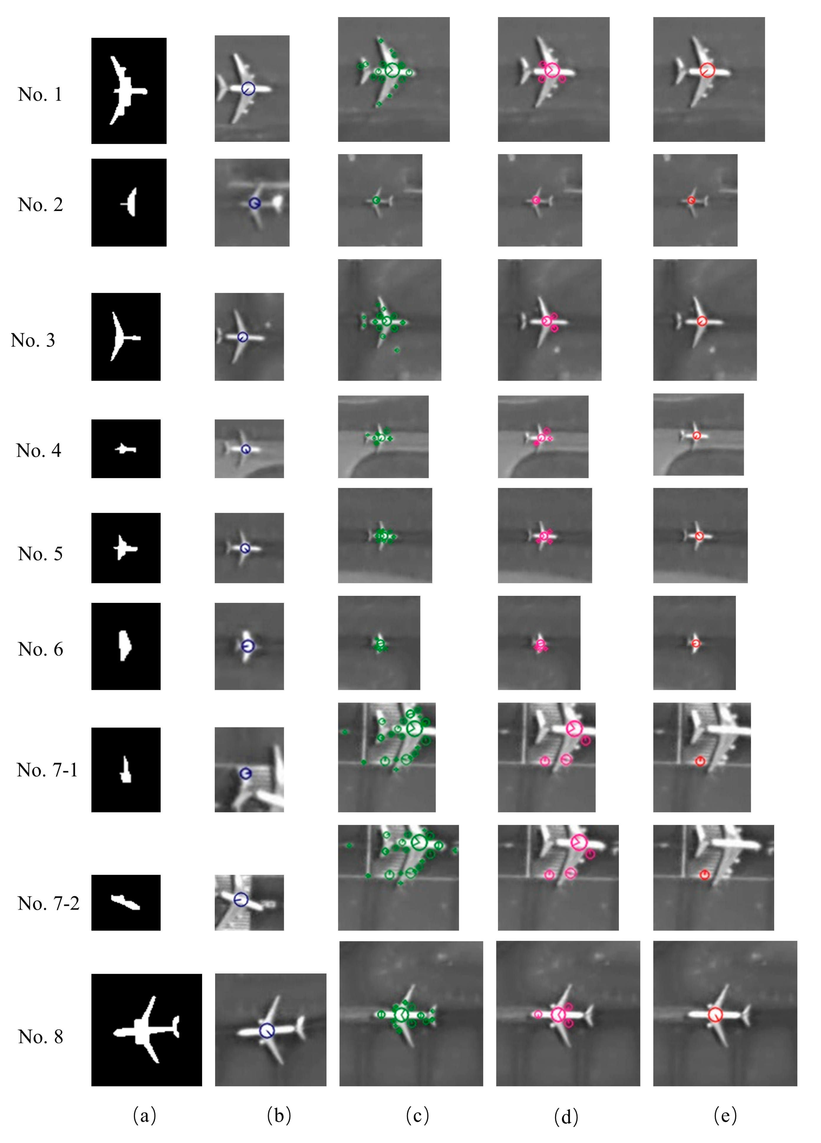
To save space, Figure 7 only shows the tracking result in the last tracking sample frame by using our P-SIFT keypoint matching algorithm. The figure contains nine rows because the moving Airplane 7 is detected as two parts. Masks of detected airplanes are presented in Figure 7a. Figure 7b shows P-SIFT keypoints (blue circles) of these airplanes extracted from their templates. Figure 7c shows all SIFT keypoints (green circles) obtained from the ROS in the last tracking sample frame. The five candidate SIFT keypoints (magenta circles) chosen based on the scale variable are shown in Figure 7d. If a ROS has fewer than five SIFT keypoints, all keypoints are selected as candidates. By calculating the feature vector similarity between each candidate in Figure 7d and the P-SIFT keypoint in Figure 7b, the most matched SIFT keypoint in each ROS is determined (Figure 7e). These matched SIFT keypoints (red circles) represent the tracked locations of moving airplanes in the last tracking sample frame.
For moving Airplane 1–6 and 8, their locations are successfully tracked. For moving Airplane 7, our P-SIFT keypoint matching algorithm fails to track them (7-1 and 7-2 in Figure 7). For the smaller part of moving Airplane 7 (7-1 in Figure 7), its P-SIFT keypoint has a very small-scale variable. A candidate set of five keypoints is insufficient to include its P-SIFT. This problem may be easily solved by selecting more candidates. However, for both parts of moving Airplane 7, the feature vectors of their P-SIFT keypoints from the templates are significantly affected by the surrounding zebra crossing. As a result, the candidate SIFT keypoints on the zebra crossing are mistakenly matched, rather than the correct ones on the airplane.
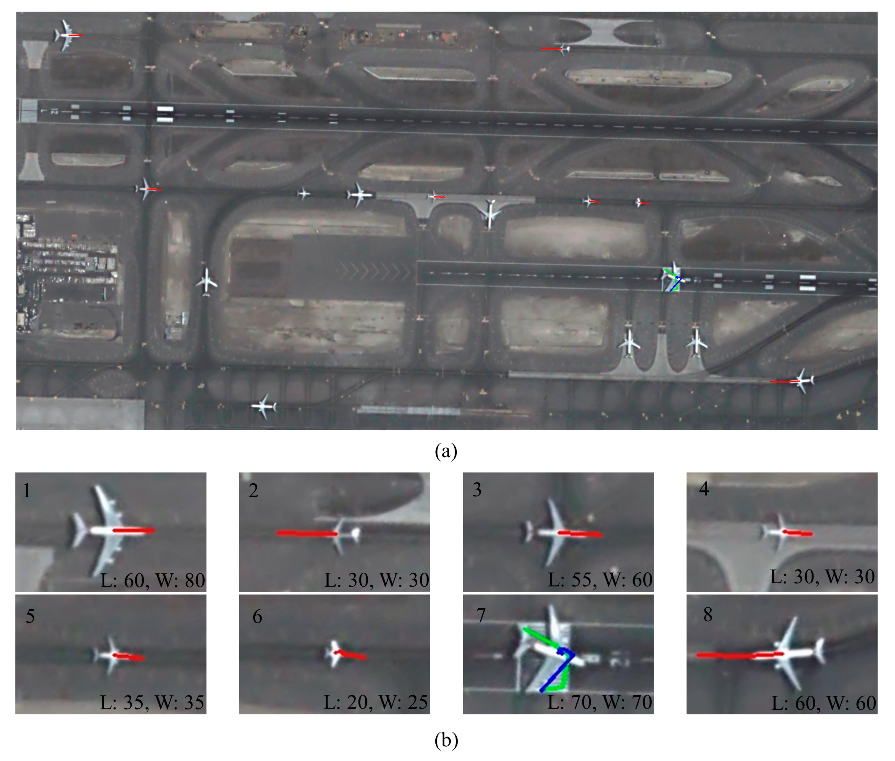
The trajectory for each moving airplane is depicted by sequentially connecting their tracked locations in each sampled tracking frame. For better visualization, these trajectories are drawn on the true-color frame of F0 (Figure 8a) with their zoomed-in views in Figure 8b. For moving Airplane 1–6 and 8, their trajectories (shown by red lines) agree well with the observation of the original video. The movement of moving Airplane 7 is presented by two trajectories (green and blue lines), but neither of them can represent the correct trajectory of this moving airplane. The movement properties of moving Airplane 1–6 and 8, including dynamic speed, average speed, and total distance traveled, are given in Table 3. It reveals that moving Airplane 5 and 8 have the lowest and highest speeds, respectively, and Airplane 1 is slowing down, whereas Airplane 2 and 3 are accelerating. Moreover, an incorrectly tracked location is found for Airplane 4 at the 19th second of the video. During four seconds (17–21 s), the computed dynamic speed of this airplane increases from 1 to 7 m/s and then decreases to 2.5 m/s. A possible reason for obtaining this incorrect dynamic speed is that the detected P-SIFT keypoint on this airplane may shift for a few pixels at the 19th second.
5. Discussion
5.1. Computational Efficiency
The algorithms for moving airplane detection and tracking were written in Python and implemented on a PC with a 3.41 GHz CPU and 16G memory running Windows 10. Since IPGBBS was implemented with matrix operations, the number of moving airplanes in each frame has little impact on computational efficiency. Our experiment found that the developed IPGBBS algorithm is able to process more than 58 frames per second. In the tracking stage, the average time for tracking an airplane in a new frame is about 5 ms. If moving airplanes were tracked once per second, our tracking algorithm could achieve real-time tracking for up to 200 airplanes altogether. Furthermore, the tracking efficiency can be further boosted by implementing in a parallel processing system.
5.2. Data Availability
Currently, the bottleneck of satellite videography research is data availability, and many practical values of the satellite videography are yet to be explored. Due to the limited data availability, we are not able to test our method in more challenging conditions such as heavy cloud and dust cover. Encouragingly, Chang Guang Satellite Technology Co., Ltd., the vendor of Jilin-1 satellite videos, has recently released its mid- to long-term plan. Specifically, the midterm plan aims to establish a constellation of sixty satellites by 2030 with a revisit capability of 30 min. The long-term plan is to have 138 satellites in orbit to achieve a 10-min revisit capability for any location on Earth after 2030. Therefore, the developed method possesses great potentials in the foreseeable future.
6. Conclusions
This paper describes an innovative method to detect and track moving airplanes in a satellite video. For moving airplane detection, we designed an IPGBBS algorithm to deal with the foreground aperture problem posed by the typically slow-moving airplanes. Furthermore, a morphological closing operation and an area filter were used to boost the detection accuracy. For moving airplane tracking, we developed a P-SIFT keypoint matching algorithm to deal with tracking uncertainties caused by intensity variation and airplane rotation. Our method was tested on a satellite video to detect and track eight moving airplanes of different sizes and dynamic statuses. The IPGBBS algorithm achieved the best detection accuracy compared with state-of-the-art algorithms. Specifically, all targets were successfully detected with the minimum number of FPs. The P-SIFT keypoint matching algorithm successfully tracked seven out of eight airplanes. Additionally, the movement trajectories of the airplanes and their dynamic properties were estimated. Future work will concentrate on further testing and improving the robustness of the detection and tracking algorithms against cloudy and dusty conditions as well as the camouflage effect.
Author Contributions
Conceptualization, F.S., F.Q., and X.L.; methodology, F.S. and Y.T.; resources, R.Z. and C.Y.; writing—original draft preparation, F.S. and Y.T.; writing—review and editing, F.Q., C.Y., and R.Z.; and supervision, F.Q. All authors have read and agreed to the published version of the manuscript.
Funding
This research was funded by the National Science Foundation (NSF) grant number BCS-1826839.
Acknowledgments
The imagery used in this paper to show the study area was provided by ESRI basemap.
Conflicts of Interest
The authors declare no conflict of interest.
References
- Shao, J.; Du, B.; Wu, C.; Zhang, L. Can we track targets from space? A hybrid kernel correlation filter tracker for satellite video. IEEE Trans. Geosci. Remote Sens. 2019, 57, 8719–8731. [Google Scholar] [CrossRef]
- Ahmadi, S.A.; Ghorbanian, A.; Mohammadzadeh, A. Moving vehicle detection, tracking and traffic parameter estimation from a satellite video: A perspective on a smarter city. Int. J. Remote Sens. 2019, 40, 8379–8394. [Google Scholar] [CrossRef]
- Mou, L.; Zhu, X.; Vakalopoulou, M.; Karantzalos, K.; Paragios, N.; Le Saux, B.; Moser, G.; Tuia, D. Multitemporal very high resolution from space: Outcome of the 2016 IEEE GRSS data fusion contest. IEEE J. Sel. Top. Appl. Earth Obs. Remote Sens. 2017, 10, 3435–3447. [Google Scholar] [CrossRef] [Green Version]
- Zhang, J.; Jia, X.; Hu, J. Motion flow clustering for moving vehicle detection from satellite high definition video. In Proceedings of the International Conference on Digital Image Computing: Techniques and Applications (DICTA), Sydney, Australia, 29 November–1 December 2017; pp. 1–7. [Google Scholar]
- Yang, T.; Wang, X.; Yao, B.; Li, J.; Zhang, Y.; He, Z.; Duan, W. Small moving vehicle detection in a satellite video of an urban area. Sensors 2016, 16, 1528. [Google Scholar] [CrossRef] [Green Version]
- Mou, L.; Zhu, X. Spatiotemporal scene interpretation of space videos via deep neural network and tracklet analysis. In Proceedings of the IEEE International Geoscience and Remote Sensing Symposium (IGARSS), Bejing, China, 10–15 July 2016; pp. 1823–1826. [Google Scholar]
- Kopsiaftis, G.; Karantzalos, K. Vehicle detection and traffic density monitoring from very high resolution satellite video data. In Proceedings of the IEEE International Geoscience and Remote Sensing Symposium (IGARSS), Milan, Italy, 26–31 July 2015; pp. 1881–1884. [Google Scholar]
- Vakalopoulou, M.; Platias, C.; Papadomanolaki, M.; Paragios, N.; Karantzalos, K. Simultaneous registration, segmentation and change detection from multisensor, multitemporal satellite image pairs. In Proceedings of the IEEE International Geoscience and Remote Sensing Symposium (IGARSS), Bejing, China, 10–15 July 2016; pp. 1827–1830. [Google Scholar] [CrossRef] [Green Version]
- Kelbe, D.; White, D.; Hardin, A.; Moehl, J.; Phillips, M. Sensor-agnostic photogrammetric image registration with applications to population modeling. Procedings of the IEEE International Geoscience and Remote Sensing Symposium (IGARSS), Bejing, China, 10–15 July 2016; pp. 1831–1834. [Google Scholar] [CrossRef]
- Ahmadi, S.A.; Mohammadzadeh, A. A simple method for detecting and tracking vehicles and vessels from high resolution spaceborne videos. In Proceedings of the Joint Urban Remote Sensing Event (JURSE), Dubai, UAE, 6–8 March 2017; pp. 1–4. [Google Scholar] [CrossRef]
- Shao, J.; Du, B.; Wu, C.; Zhang, L. Tracking objects from satellite videos: A velocity feature based correlation filter. IEEE Trans. Geosci. Remote Sens. 2019, 57, 7860–7871. [Google Scholar] [CrossRef]
- Piccardi, M. Background subtraction techniques: A review. In Proceedings of the IEEE International Conference on Systems, Man and Cybernetics, The Hague, The Netherlands, 10–13 October 2004; Volume 4, pp. 3099–3104. [Google Scholar]
- Elhabian, S.Y.; El-Sayed, K.M.; Ahmed, S.H. Moving object detection in spatial domain using background removal techniques-state-of-art. Recent Patents Comput. Sci. 2008, 1, 32–54. [Google Scholar] [CrossRef]
- Chris, S.; Grimson, W.E. Adaptive background mixture models for real-time tracking. In Proceedings of the IEEE Computer Society Conference on Computer Vision and Pattern Recognition, Fort Collins, CO, USA, 23–25 June 1999; Volume 2, pp. 246–252. [Google Scholar] [CrossRef]
- Kim, K.; Chalidabhongse, T.H.; Harwood, D.; Davis, L. Real-time foreground-background segmentation using codebook model. Real-Time Imag. 2005, 11, 172–185. [Google Scholar] [CrossRef] [Green Version]
- Barnich, O.; Droogenbroeck, M. Van ViBe: A universal background subtraction algorithm for video sequences. IEEE Trans. Image Process 2010, 20, 1709–1724. [Google Scholar] [CrossRef] [Green Version]
- Barnich, O.; Van Droogenbroeck, M. ViBe: A powerful random technique to estimate the background in video sequences. In Proceedings of the 2009 IEEE International Conference on Acoustics, Speech and Signal Processing, Taipei, Taiwan, 19–24 April 2009; pp. 945–948. [Google Scholar]
- Koga, Y.; Miyazaki, H.; Shibasaki, R. A method for vehicle detection in high-resolution satellite images that uses a region-based object detector and unsupervised domain adaptation. Remote Sens. 2020, 12, 575. [Google Scholar] [CrossRef] [Green Version]
- Zhang, X.; Zhu, X. An efficient and scene-adaptive algorithm for vehicle detection in aerial images using an improved YOLOv3 framework. ISPRS Int. J. Geo-Inf. 2019, 8, 483. [Google Scholar] [CrossRef] [Green Version]
- Zheng, K.; Wei, M.; Sun, G.; Anas, B.; Li, Y. Using vehicle synthesis generative adversarial networks to improve vehicle detection in remote sensing images. ISPRS Int. J. Geo-Inf. 2019, 8, 390. [Google Scholar] [CrossRef] [Green Version]
- Audebert, N.; Le Saux, B.; Lefèvre, S. Segment-before-detect: Vehicle detection and classification through semantic segmentation of aerial images. Remote Sens. 2017, 9, 368. [Google Scholar] [CrossRef] [Green Version]
- Jain, S.D.; Xiong, B.; Grauman, K. FusionSeg: Learning to combine motion and appearance for fully automatic segmentation of generic objects in videos. In Proceedings of the IEEE Conference on Computer Vision and Pattern Recognition (CVPR), Honolulu, HI, USA, 21–26 July 2017; pp. 2117–2126. [Google Scholar] [CrossRef]
- Perazzi, F.; Khoreva, A.; Benenson, R.; Schiele, B.; Sorkine-Hornung, A. Learning video object segmentation from static images. In Proceedings of the IEEE Conference on computer vision and pattern recognition, Honolulu, HI, USA, 22–25 July 2017; pp. 3491–3500. [Google Scholar]
- You, S.; Zhu, H.; Li, M.; Li, Y. A review of visual trackers and analysis of its application to mobile robot. arXiv 2019, arXiv:1910.09761. [Google Scholar]
- Pan, Z.; Liu, S.; Fu, W. A review of visual moving target tracking. Multimed. Tools Appl. 2017, 76, 16989–17018. [Google Scholar] [CrossRef]
- Lewis, J.P. Fast Normalized Cross-Correlation. 1995. Available online: https://citeseerx.ist.psu.edu/viewdoc/summary?doi=10.1.1.21.6062 (accessed on 5 March 2020).
- Liwei, W.; Yan, Z.; Jufu, F. On the Euclidean distance of images. IEEE Trans. Pattern Anal. Mach. Intell. 2005, 27, 1334–1339. [Google Scholar] [CrossRef]
- Nakhmani, A.; Tannenbaum, A. A new distance measure based on generalized Image normalized cross-correlation for robust video tracking and image recognition. Pattern Recognit. Lett. 2013, 34, 315–321. [Google Scholar] [CrossRef] [Green Version]
- Tsai, D.-M.; Tsai, Y.-H. Rotation-invariant pattern matching with color ring-projection. Pattern Recognit. 2002, 35, 131–141. [Google Scholar] [CrossRef]
- Hu, M.K. Visual pattern recognition by moment invariants. IRE Trans. Inf. Theory 1962, 8, 179–187. [Google Scholar]
- Goshtasby, A. Template Matching in Rotated Images. IEEE Trans. Pattern Anal. Mach. Intell. 1985, 3, 338–344. [Google Scholar] [CrossRef]
- Kaur, A.; Singh, C. Automatic cephalometric landmark detection using Zernike moments and template matching. Signal Image Video Process. 2015, 9, 117–132. [Google Scholar] [CrossRef]
- Ullah, F.; Kaneko, S. Using orientation codes for rotation-invariant template matching. Pattern Recognit. 2004, 37, 201–209. [Google Scholar] [CrossRef]
- Choi, M.S.; Kim, W.Y. A novel two stage template matching method for rotation and illumination invariance. Pattern Recognit. 2002, 35, 119–129. [Google Scholar] [CrossRef]
- Wang, L.; Liu, T.; Wang, G.; Chan, K.L.; Yang, Q. Video tracking using learned hierarchical features. IEEE Trans. Image Process. 2015, 24, 1424–1435. [Google Scholar] [CrossRef] [PubMed]
- Choi, J.; Chang, H.J.; Fischer, T.; Yun, S.; Lee, K.; Jeong, J.; Demiris, Y.; Choi, J.Y. Context-aware deep feature compression for high-speed visual tracking. In Proceedings of the IEEE/CVF Conference on Computer Vision and Pattern Recognition, Salt Lake City, UT, USA, 18–23 June 2018; pp. 479–488. [Google Scholar] [CrossRef] [Green Version]
- Dicle, C.; Camps, O.I.; Sznaier, M. The way they move: Tracking multiple targets with similar appearance. In Proceedings of the IEEE International Conference on Computer Vision, Sidney, Australia, 1–8 December 2013; pp. 2304–2311. [Google Scholar] [CrossRef] [Green Version]
- Luo, W.; Xing, J.; Milan, A.; Zhang, X.; Liu, W.; Zhao, X.; Kim, T.-K. Multiple object tracking: A literature review. arXiv 2017, arXiv:1409.7618. [Google Scholar]
- Javed, O.; Shah, M.; Shafique, K. A hierarchical approach to robust background subtraction using color and gradient information. In Proceedings of the Workshop on Motion and Video Computing, Orlando, FL, USA, 9 December 2003. [Google Scholar] [CrossRef]
- Toyama, K.; Krumm, J.; Brumitt, B.; Meyers, B. Wallflower: Principles and practice of background maintenance. In Proceedings of the Seventh IEEE International Conference on Computer Vision, Kerkyra, Greece, 20–27 September 1999; pp. 255–261. [Google Scholar]
- Cristani, M.; Farenzena, M.; Bloisi, D.; Murino, V. Background subtraction for automated multisensor surveillance: A comprehensive review. EURASIP J. Adv. Signal. Process. 2010, 2010, 1–24. [Google Scholar] [CrossRef] [Green Version]
- Juan, L.; Gwon, L. A comparison of sift, pca-sift and surf. Int. J. Signal. Process. 2007, 8, 169–176. [Google Scholar] [CrossRef]
- Lowe, D.G. Distinctive Image Features from Scale-Invariant Keypoints. Int. J. Comput. Vis. 2004, 60, 91–110. [Google Scholar] [CrossRef]
Figure 1.
Study area and Jilin-1 satellite video frames: (a) the ESRI base map showing the study area of the Dubai International Airport; and (b,c) the first and last frames of the Jilin-1 satellite video. All eight moving airplanes are labeled.
Figure 1.
Study area and Jilin-1 satellite video frames: (a) the ESRI base map showing the study area of the Dubai International Airport; and (b,c) the first and last frames of the Jilin-1 satellite video. All eight moving airplanes are labeled.

Figure 2.
Moving airplane detection with a background model of different adaption strategies: (a) both the foreground and background are adapted with the same learning rate; (b) only the background is adapted; (c) the foreground is adapted with a smaller learning rate than the background; and (d) the detection in (c) is further boosted by a morphological closing operation.

Figure 3.
The extraction of extrema from a DOG. A pixel (red) is compared with eight neighbors in the current DOG and nine neighbors (all pixels in green) in the DOG above and below, respectively.
Figure 3.
The extraction of extrema from a DOG. A pixel (red) is compared with eight neighbors in the current DOG and nine neighbors (all pixels in green) in the DOG above and below, respectively.

Figure 4.
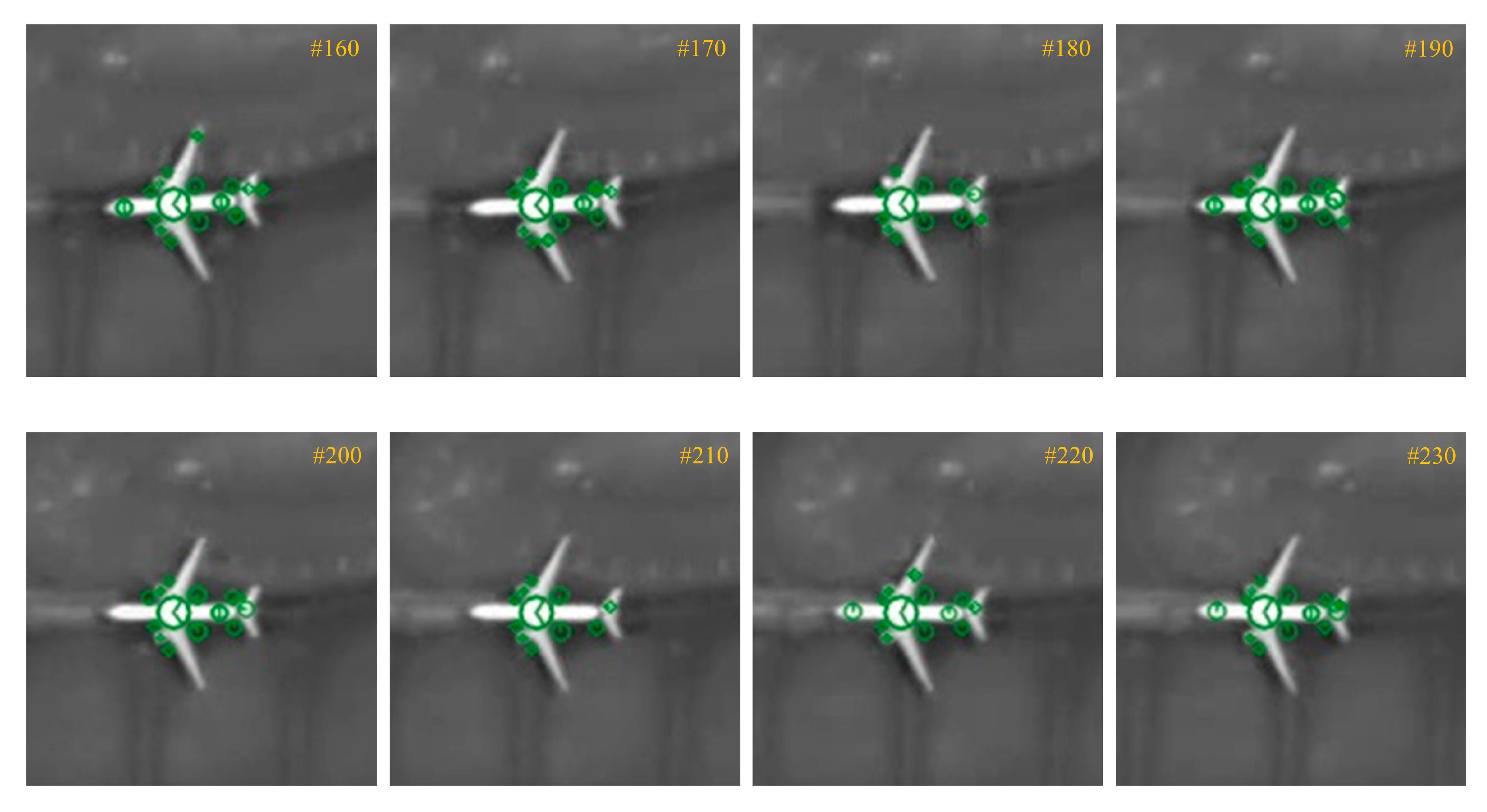
The SIFT keypoints of moving Airplane 8 extracted from different frames. The number in each subfigure represents the frame ID in the test video. Each SIFT keypoint is represented by a circle with an angled radius.
Figure 4.
The SIFT keypoints of moving Airplane 8 extracted from different frames. The number in each subfigure represents the frame ID in the test video. Each SIFT keypoint is represented by a circle with an angled radius.

Figure 5.
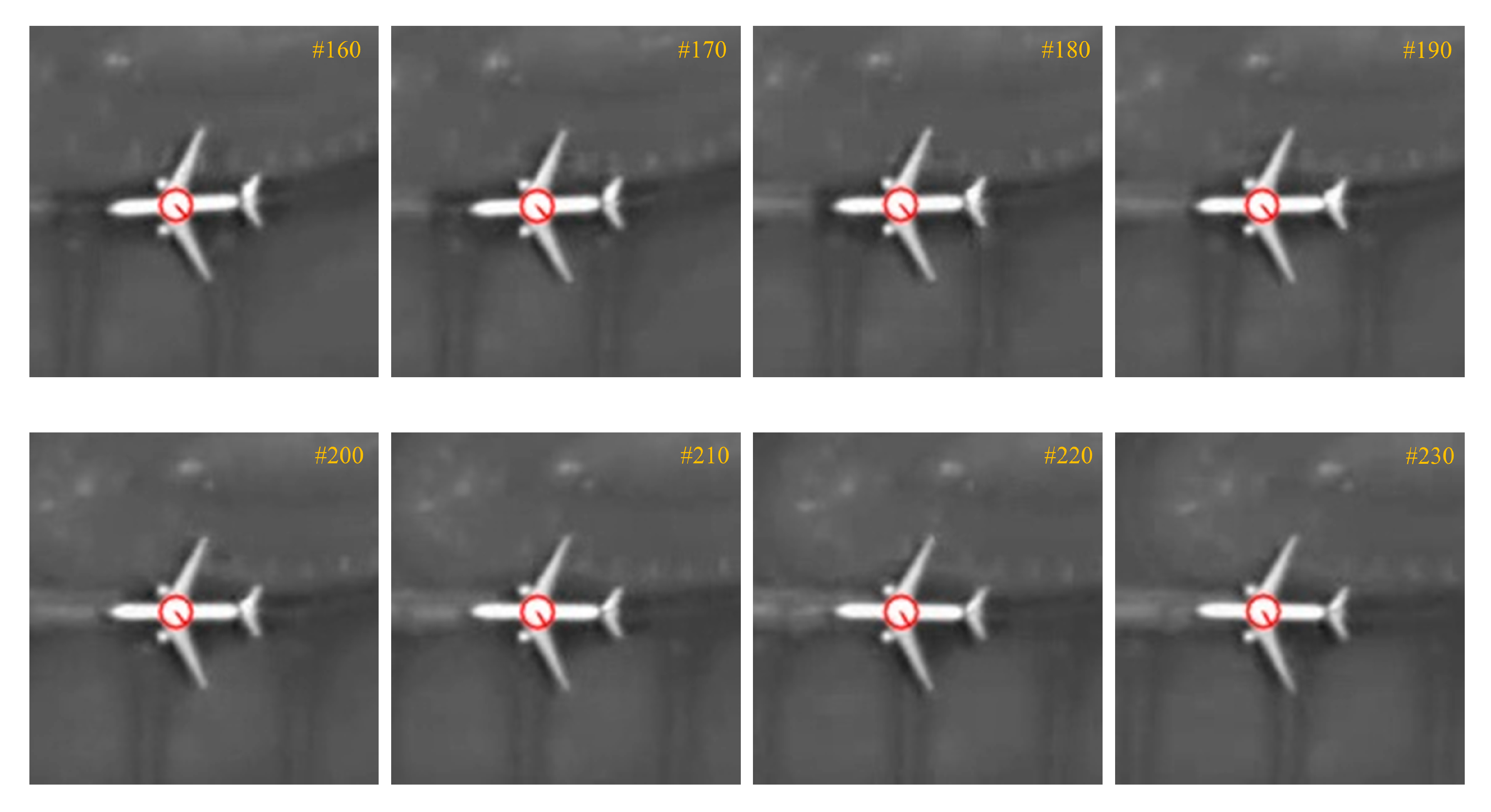
Extracted P-SIFT keypoint of the moving Airplane 8 shown in Figure 4. The number in each subfigure represents the frame ID in the test video.
Figure 5.
Extracted P-SIFT keypoint of the moving Airplane 8 shown in Figure 4. The number in each subfigure represents the frame ID in the test video.

Figure 6.
Initial and boosted results of moving airplane detection by four algorithms: (a) ground reference; (b) Codebook; (c) MoG; (d) ViBe; and (e) our IPGBBS algorithm.
Figure 6.
Initial and boosted results of moving airplane detection by four algorithms: (a) ground reference; (b) Codebook; (c) MoG; (d) ViBe; and (e) our IPGBBS algorithm.

Figure 7.
Tracking results of the developed P-SIFT keypoint matching algorithm: (a) masks of moving airplanes; (b) P-SIFT keypoints (blue circles) the templates extracted from F0; (c) SIFT keypoints (green circles) inside the ROS extracted from the last tracking sample frame; (d) SIFT keypoint candidates (magenta circles) selected from (c); and (e) the most matched SIFT keypoint (red circles).

Figure 8.
Airplane trajectories estimated from the 150th frame to the last (250th frame): (a) trajectories of eight moving airplanes delineated on the true-color 150th video frame, and (b) zoomed-in view for each trajectory. The approximate length (L) and width (W) of each airplane are illustrated in meters. The trajectories of Airplane 1–6 and 8 are presented by red lines, and trajectories of the two parts of Airplane 7 are represented by green and blue lines.


Table 1.
Suggested parameters for the IPGBBS algorithm.
| Parameter | Description | Value |
|---|---|---|
| σ0 | The initial standard deviation for the Gaussian background model | 30 |
| αb | The learning rate for adapting background pixels | 0.01 |
| αf | The learning rate for adapting foreground pixels | 0.001 |
| φ | The threshold to detect foreground pixels | 3 |
Table 2.
Accuracy assessment of four moving object detection algorithms.
| Algorithm | FP Count | Recall | Precision | F1 Score |
|---|---|---|---|---|
| Initial Detection | ||||
| Codebook | 37 | 0.125 | 0.026 | 0.043 |
| MoG | 7866 | 1 | 0.001 | 0.002 |
| ViBe | 129 | 1 | 0.058 | 0.110 |
| IPGBBS | 34 | 1 | 0.191 | 0.321 |
| Boosted Detection | ||||
| Codebook | 1 | 0.125 | 0.500 | 0.200 |
| MoG | 199 | 0.750 | 0.029 | 0.056 |
| ViBe | 2 | 1.000 | 0.800 | 0.889 |
| IPGBBS | 1 | 1.000 | 0.890 | 0.942 |
Table 3.
Movement properties of Airplane 1–6 and 8.
| Airplane ID | Dynamic Speed (m/s) | Average Speed (m/s) | Total Distance (m) | ||||
|---|---|---|---|---|---|---|---|
| 17 s | 19 s | 21 s | 23 s | 25 s | |||
| 1 | 3.63 | 3.53 | 3.49 | 3.27 | 2.76 | 3.34 | 33.37 |
| 2 | 4.25 | 4.61 | 4.95 | 5.37 | 5.41 | 4.92 | 49.17 |
| 3 | 3.16 | 3.44 | 3.6 | 3.64 | 4.01 | 3.57 | 35.70 |
| 4 | 1 | 7.05 | 2.51 | 1.81 | 1.17 | 2.71 | 27.06 |
| 5 | 2.41 | 2.49 | 2.47 | 2.45 | 2.56 | 2.48 | 24.78 |
| 6 | 2.03 | 3.04 | 2.51 | 2.61 | 2.77 | 2.59 | 25.92 |
| 8 | 7.21 | 7.4 | 7.06 | 7.16 | 6.81 | 7.13 | 71.26 |
Frame rate: 10 fps; pixel resolution: 1 m.
© 2020 by the authors. Licensee MDPI, Basel, Switzerland. This article is an open access article distributed under the terms and conditions of the Creative Commons Attribution (CC BY) license (http://creativecommons.org/licenses/by/4.0/).
Share and Cite
MDPI and ACS Style
Shi, F.; Qiu, F.; Li, X.; Tang, Y.; Zhong, R.; Yang, C. A Method to Detect and Track Moving Airplanes from a Satellite Video. Remote Sens. 2020, 12, 2390. https://doi.org/10.3390/rs12152390
AMA Style
Shi F, Qiu F, Li X, Tang Y, Zhong R, Yang C. A Method to Detect and Track Moving Airplanes from a Satellite Video. Remote Sensing. 2020; 12(15):2390. https://doi.org/10.3390/rs12152390
Chicago/Turabian StyleShi, Fan, Fang Qiu, Xiao Li, Yunwei Tang, Ruofei Zhong, and Cankun Yang. 2020. "A Method to Detect and Track Moving Airplanes from a Satellite Video" Remote Sensing 12, no. 15: 2390. https://doi.org/10.3390/rs12152390
Note that from the first issue of 2016, this journal uses article numbers instead of page numbers. See further details here.