Article

Using Linear Regression, Random Forests, and Support Vector Machine with Unmanned Aerial Vehicle Multispectral Images to Predict Canopy Nitrogen Weight in Corn

1
Department of Geography, the University of Western Ontario, London, ON N6A 3K7, Canada
2
The Institute for Earth and Space Exploration, the University of Western Ontario, London, ON N6A 3K7, Canada
3
Faculty of Forestry and Environmental Management, University of New Brunswick, Fredericton, NB E3B 5A3, Canada
*
Author to whom correspondence should be addressed.
Remote Sens. 2020, 12(13), 2071; https://doi.org/10.3390/rs12132071
Submission received: 2 June 2020 / Revised: 21 June 2020 / Accepted: 25 June 2020 / Published: 27 June 2020
(This article belongs to the Special Issue Environmental Mapping Using Remote Sensing)

Abstract

:
The optimization of crop nitrogen fertilization to accurately predict and match the nitrogen (N) supply to the crop N demand is the subject of intense research due to the environmental and economic impact of N fertilization. Excess N could seep into the water supplies around the field and cause unnecessary spending by the farmer. The drawbacks of N deficiency on crops include poor plant growth, ultimately reducing the final yield potential. The objective of this study is to use Unmanned Aerial Vehicle (UAV) multispectral imagery to predict canopy nitrogen weight (g/m2) of corn fields in south-west Ontario, Canada. Simple/multiple linear regression, Random Forests, and support vector regression (SVR) were established to predict the canopy nitrogen weight from individual multispectral bands and associated vegetation indices (VI). Random Forests using the current techniques/methodologies performed the best out of all the models tested on the validation set with an R2 of 0.85 and Root Mean Square Error (RMSE) of 4.52 g/m2. Adding more spectral variables into the model provided a marginal improvement in the accuracy, while extending the overall processing time. Random Forests provided marginally better results than SVR, but the concepts and analysis are much easier to interpret on Random Forests. Both machine learning models provided a much better accuracy than linear regression. The best model was then applied to the UAV images acquired at different dates for producing maps that show the spatial variation of canopy nitrogen weight within each field at that date.

Graphical Abstract

1. Introduction

Precision agriculture (PA) is a farming management technique that requires detailed information on crop status. One of the important crop status indicators is the crop nitrogen (N) weight because nitrogen is the main plant nutrient needed for producing the chlorophyll, which has a direct impact on the plant photosynthesis and thus on crop growth and yield [1]. Therefore, there is a need to understand the spatial distribution of crop nitrogen for better use of fertilizers. Ultimately, this information leads to a better yield among the crops and reduces costs for the farmer by matching the fertilizer supply to its demand [2,3]. Traditionally, farmers used to rely on historical weather data, such as precipitation and temperature, and their past experiences, such as crop yields, to make decisions on their fertilizer operations for the upcoming season [4]. Today, there have been many advances in technology, such as remote sensing data and machine learning algorithms, that can potentially aid farmers’ decision making on fertilizer application. Remote sensing-based methods used to measure crop nitrogen are typically better than the traditional ground-based methods. Ground-based methods require intensive field data collection, which can be time-consuming, destructive, and limited to a small spatial area, making it impractical for fast and efficient results. Remote sensing-based methods are required for most agricultural fields in Canada, given that they can reach up to hundreds of ha in size. Remote sensing methods are non-destructive, can cover large spatial areas, and have been increasingly used for crop monitoring in precision agriculture. Crop monitoring based on remote sensing data can use spaceborne or airborne images, but these types of high-resolution imagery are either costly or difficult to obtain [5]. Also, they have limited applicability in precision agriculture because of the too coarse temporal and spatial resolutions of the imagery [6,7]. Alternatively, free-of-charge Sentinel-1 Synthetic Aperture Radar (SAR) imagery could be used to monitor nitrogen status but does not provide enough spatial resolution (10 m) for precise small-scaled applications [8]. Bagheri et al. [9] also found it difficult to differentiate levels of nitrogen status in corn fields using a 15 m Advanced Spaceborne Thermal Emission and Reflection Radiometer (ASTER) multispectral satellite imagery. An alternative is to use Unmanned Aerial Vehicle (UAV) imagery. The development and application of UAV imagery have increased in the past decade, filling in gaps between satellite imagery, aerial photography, and field samples [10,11]. Image acquisition with UAV can be deployed quickly and repeatedly, at a low cost, and with greater flexibility [12,13]. The temporal resolution of UAVs is superior to the satellite and aerial photography platforms, which is easily defined by the user [14,15]. The low cost of UAVs could also be convinced without the use of purchasing ground control points (GCPs) [14].
The focus of this study is to test whether UAV multispectral imagery can be used to retrieve the crop nitrogen status over corn fields from a perspective of precision nitrogen fertilization. The spatial and temporal variations of the images we acquired were determined in order to match the crop requirements of nitrogen as closely as possible. One common remote sensing technique to estimate nitrogen content at the canopy level is the Radiative Transfer Model (RTM), which estimates the chlorophyll or nitrogen content by describing the interaction between the sun’s light and the crop canopy. An example of an RTM is the PROSAIL model, which uses various parameters at the leaf and canopy level and can be mathematically inverted to retrieve both chlorophyll and nitrogen content from spectral data [1,16,17,18,19]. Other sets of remote sensing methods are empirical methods, such as machine learning algorithms, or simple/multiple-linear regression to retrieve crop nitrogen from canopy spectral data [16]. This paper used the second set of methods because empirical estimation has already been proven to be easier in estimating nitrogen than the PROSAIL model, given that an RTM requires the calibration of numerous parameters [20]. In this study, we tested three empirical methods: (1) linear regression, (2) Random Forests, and (3) support vector regression (SVR) to statistically relate spectral measurements and canopy-level crop nitrogen weight in the case of two corn fields located in southwest Ontario, Canada. Many studies on predicting nitrogen were conducted in a controlled experimental condition and predicted nitrogen values at the leaf level [21,22,23,24], while few studies have been performed on real field conditions [25]. As already shown in Liu et al. [3], it is better to use more than one spectral variable for estimating crop nitrogen. Therefore, multiple linear regression, Random Forests, and SVR was used in this paper to predict canopy nitrogen using a variety of spectral variables.
The first regression method is a traditional regression approach that has two major assumptions (multicollinearity and linear relationship). Most studies using UAV imagery have used linear regressions to estimate nitrogen status from vegetation indices (VIs) [13]. The latter two approaches are machine learning techniques that have been advanced in recent years and are unaffected by the multicollinearity and linear relationship assumptions. In addition, they can handle overfitting [13,26,27]. Overfitting is a common problem in machine learning where the models produced perform poorly on unseen data. Random Forests has become popular recently within the remote sensing research community for classification and regression purposes. The variable importance plot provided by the Random Forests algorithm is very successful in identifying the most relevant input data in the model [27,28]. Therefore, we used the Random Forests variable importance plots to identify the most important variables for canopy nitrogen estimation and adjusted the model parameters accordingly. Random Forests modeling has been found to perform very well out of all the non-parametric methods in various studies to monitor nitrogen content in wheat [3], rice [13], and citrus trees [28]. Random Forests was also the most accurate machine learning approach for monitoring corn yield, which is related to crop nitrogen status [26]. Support vector modeling has also been popular in estimating nitrogen status due to its strong ability to decorrelate the input variables and can work with non-linear relationships [29,30,31]. SVR modeling has been found to predict nitrogen concentration with high accuracy in bokchoy [29], wheat [30], and corn [31].
Ideally, the relationship between the spectral data and the canopy nitrogen weight should be linear because there should be only one canopy nitrogen weight estimation for each level of input data, given that the relationship will be used to calibrate an N fertilizer sprayer that needs to have an exact determination of the crop N fertilization level. However, when the canopy becomes dense, the relationship can saturate and become non-linear. This is the case when using some VIs, such as the standard normalized difference vegetation index (NDVI), green NDVI, red edge NDVI, and modified transformed vegetation index 2 (MTVI2), which has been shown to saturate at high canopy densities [32]. Therefore, this study tested the ability of Random Forests and SVR to work with non-linear saturated data, particularly when combining datasets throughout the growing cycle.
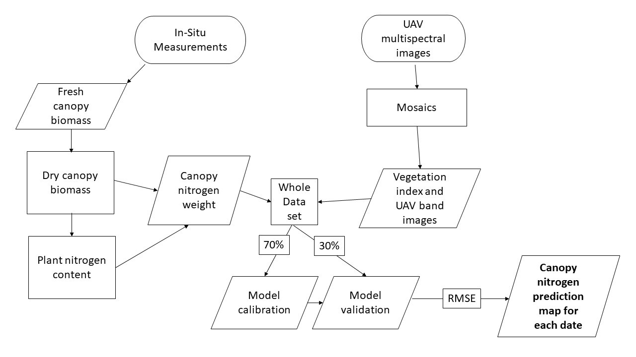
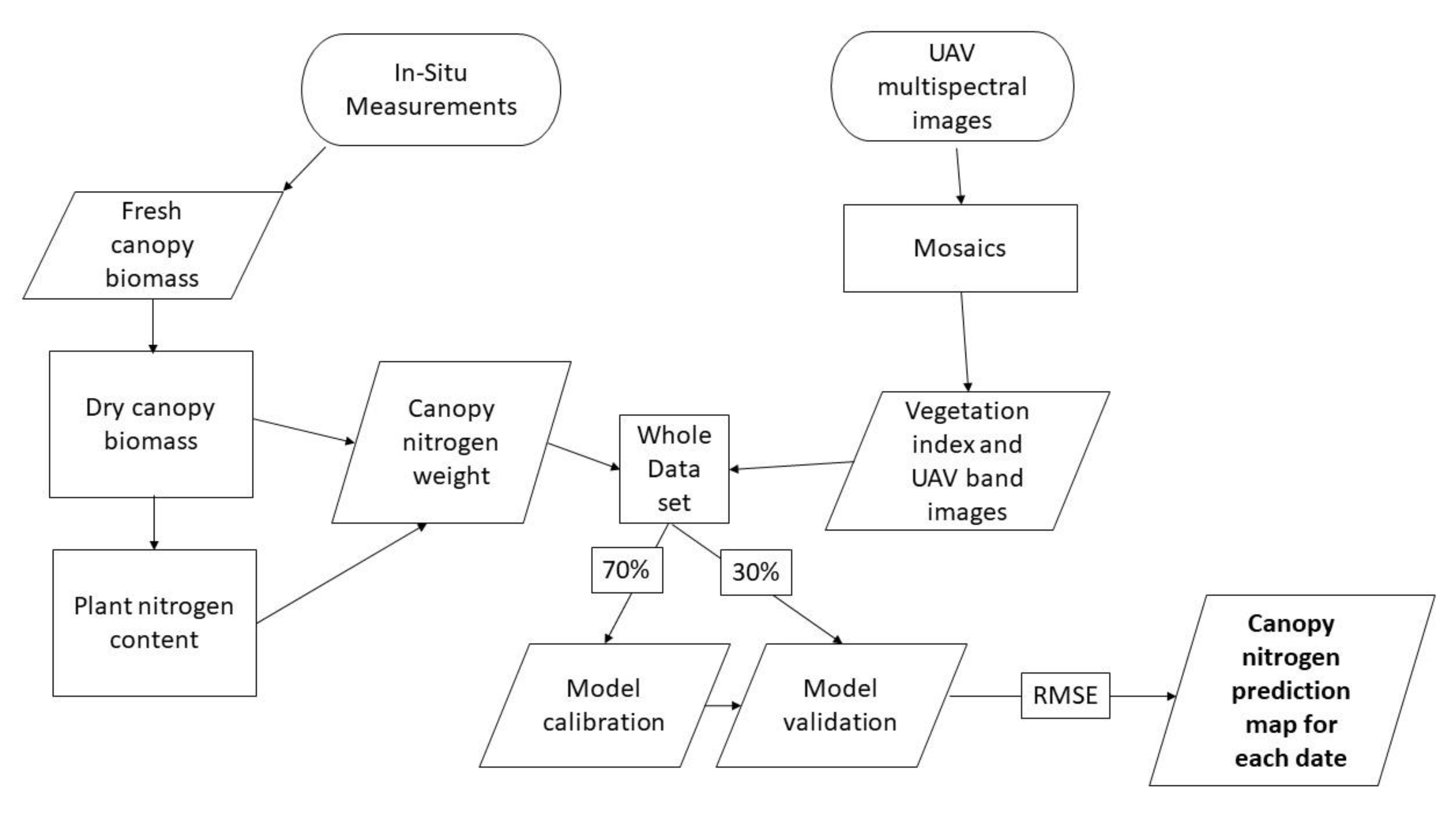
The best performing model was applied to the UAV imagery for mapping crop nitrogen content at the field level. Deng et al. [33] found that mounting narrowband multispectral cameras on UAVs acquire images with far better quality than broadband multispectral cameras. Therefore, the objectives of this study are to (i) generate machine learning models to predict crop nitrogen weight in corn fields using UAV multispectral imagery, (ii) determine which individual MicaSense spectral bands and VIs have the most influence on the Random Forests decision tree when predicting nitrogen, (iii) generate nitrogen prediction maps by applying the best model to the entire UAV image and analyze whether the UAV images are able to detect any spatial variation of nitrogen within the fields. The study evaluates three different modeling approaches for predicting nitrogen in corn over different dates and growth stages using UAV multispectral imagery. The best algorithm not only fills the research gap between monitoring nitrogen and UAVs, but also has practical meaning for future modeling study designs. Ultimately, these images should be given to farmers in highly accurate, quick, and timely manner field information for their precision nitrogen fertilization management.

2. Materials and Methods

2.1. Study Area

The study site is located in Melbourne, Ontario, Canada (Figure 1). This region is in the humid continental climate zone in Canada and the summers are typically hot and humid, with an average temperature of 27 °C during the fieldwork month of July 2019. The study site is dominated by agricultural land with very little urban use. The closest large urban center is London, Ontario, just 30 km east of the study site. Corn is generally planted in May just before the summer and typically harvested in late October/early November once the crop is dried and the starch content is high.
We collected field data from two corn (Zea mays) fields (labelled as JJ and Susan) in the summer of 2019. Both fields are sown with cultivars “DKC48-56RIB”. A total of six sampling dates were collected for corn, with at least a week in between each sampling date. Both corn fields together were roughly 60 ha in size and situated directly across from each other. The study fields are smaller than the average agricultural field sizes in Ontario (100 ha) [34]. However, such field sizes are large enough to avoid weak relationships in using spectral data and related VIs to predict nitrogen because smaller fields can be more affected by bare soil surrounding the fields and the mixing effect of other nearby fields [35]. Both fields were similar in topography and planted at the same time by the same grower, allowing the field data collected to be used in a single model.

2.2. Field Data

In-situ data were collected over 16 points on each corn field in June and July 2019. Whiteboard and red sticks were placed on each sample point, which was a ground control point to be identified on the UAV imagery for orthomosaicking. In-situ data included destructive biomass collection at each sampling point. Fresh biomass was measured in grams by gathering the fresh canopy in a 1 m2 block around the sampling point and placed in large plastic bags for transport. Due to the intensive work and heavy weight of the fresh corn canopy, only two plants were taken per sample point and upscaled to the number of plants in the 1 m2 block. The average row distance for corn was 75 cm and the fields typically had an average of 12–14 plants per 1 m2 area. Following the fieldwork, biomass was weighed at a fresh stage in grams, then placed in an 80 °C oven for 36–48 hours. Dried biomass weight (scaled at g/m2) was weighed then sent to A&L Canada Laboratories for plant tissue analysis. The oven-dried samples were ground into a powder form and passed through a 1 mm sieve. The leaf nitrogen content (expressed as a percentage) was then measured using the Laboratory Equipment Company (LECO) FP628 nitrogen/protein analyzer that uses the total nitrogen combustion method [36].

2.3. UAV Imagery

UAV imagery collection is optimal when collected weekly and immediately before field data collection as crop physiology and soil structure change over time (Figure 2). UAV flights were performed before the field data collection to ensure that the biomass was present at the sampling points in the imagery. UAV flights were performed on 26 June, 3 July, 10 July, 18 July, 31 and July using a MicaSense RedEdge narrowband camera mounted on a Dà-Jiāng Innovations (DJI) Matrice 100 quadcopter (Table 1). The growth stages of the corn are also described in Table 1, where V(n) represents the vegetation stage and the amount of leaves present, excluding the initial emergence leaf. Flights were flown by pilots of A&L Canada Labs Inc. over the entire fields, flown in a zigzag route and 50 m in height, and 80–85% overlap. Our past studies [32] have indicated that a high overlap is required for corn as the canopy becomes very dense in the middle-late growing season.

2.4. UAV Image Processing

Figure 3 shows the flowchart of the methodology in this study. The UAV images gathered in the summer of 2019 were processed using a photogrammetry software called Pix4Dmapper (Pix4D SA, Lausanne, Switzerland) [37]. Pix4Dmapper was used to generate an orthomosaic image of each field by stitching hundreds of different images captured during the same flight into one single 2D image and corrected for perspective. Pix4D uses the technique called Structure from Motion (SfM) and has been well-suited for UAV data as it combines images from multiple angles [15]. The mosaicked images were then exported to individual (.tif) files. The mosaic images were automatically radiometrically corrected in Pix4D with a spatial resolution of 5 cm/pixel. The mosaic images were scaled to 15 cm/pixel to reduce the computing time given the high number of pixels for a single field. For example, the Susan field scaled at 5 cm/pixel is approximately 529 million pixels per each layer.

2.5. Vegetation Indices

Reflectance values of the sample points were extracted from the MicaSense mosaic images. Five reflectance values of each sample point were acquired by the MicaSense RedEdge camera in the following bands: (1) blue, (2) green, (3) red, (4) red edge, and (5) near-infrared (Table 2) (Figure 4).
These surface reflectance values were then used to compute 29 VIs that are commonly used to estimate canopy nitrogen variables (Table 3). These indices are intended to enhance the contribution of the optical properties of the vegetation on the total spectral response of the canopy. Therefore, VIs attempt to correct any confounding factors such as reflectance of soil backgrounds in a crop, particularly at the early stages of the growth cycle [16].

2.6. Canopy Nitrogen Weight Estimation

To describe the canopy nitrogen status, we used the canopy nitrogen weight that is defined by Hansen and Schjoerring [18] as follows:
C N W = ( N p l a n t s × W d 2 ) × L N C
where CNW is the canopy nitrogen weight (g/m2), Nplants is the number of plants in the 1m2 sampling point, Wd is the dry biomass weight (g/m2) of two plants in the 1m2 sampling point, and LNC is the leaf nitrogen content (%).
Equation (1) assumes that all the leaves from a sample gathered in the field contained the same amount of nitrogen. Canopy nitrogen weight (g/m2) has the advantage of being a more absolute value, compared to plant or leaf nitrogen content (%), which is a relative value. Absolute values allow the ability to compare the results among fields and dates.
Previous studies have shown that estimating biochemical concentrations at the leaf level is difficult. Therefore, focusing on the canopy level is optimal [16]. Li et al. [25] have also found that canopy nitrogen weight is more strongly correlated with spectral data than the other agronomic variables, such as Soil Plant Analysis Development (SPAD) readings, plant nitrogen concentration%, nitrate content, and soil mineral N.

2.7. Canopy Nitrogen Weight Modeling

All modeling was performed using R programming language in R Studio (R Version 3.6.1) [62]. The first modeling approach is the simple/multiple linear regression. We avoided using all the variables in the multiple linear regression to predict nitrogen as VIs are known to be highly intercorrelated with each other. Such multicollinearity between explanatory variables reduces the accuracy of the estimates of the regression coefficients [63]. This makes the results of multiple linear regression difficult to interpret and unreliable with an increased number of variable inputs. Therefore, the linear regression model was established with the top six and top 12 most influential variables as determined by the Random Forests variable importance plot.
The second modeling approach used Random Forests. This is a decision tree nonparametric algorithm used for classification or regression. The algorithm selects a random number of samples from the training dataset chosen by the analyst. Afterward, the randomly chosen samples are used to develop a decision tree based on the most important variables. Trees are split at each node depending on the most contributing xi (ith explanatory variable) to y (response variable). For each prediction of ŷ (predicted value of the response variable), it constructs a multitude of decisions trees and outputs the average value. Figure 5 shows an example of the decision tree modeling steps for the Random Forests model using the dataset. Hyper-tuning the parameters of Random Forests was unnecessary due to the results remaining unchanged after altering the number of trees of 500 and mtry parameter at default. The parameter mtry is the number of variables used for splitting at each tree node for decision tree learning. Random Forests in R defines the mtry by dividing the number of predictive variables divided by 3.
The third modeling approach is SVR which is also a form of nonparametric modeling that defines boundaries in a high-dimensional space using a hyperplane. A hyperplane is a flat affine subspace of a dimension p-1, where p is the number of dimensions. In two dimensions, the hyperplane is a flat one-dimensional subspace (straight line) and splits the training data into different sections in a two-dimensional plot. The notion of (p-1) applies for any number of dimensions, while anything p > 3 is difficult to visualize [63]. If the relationships of the data are nonlinear, SVR uses a nonlinear kernel function. We used the Radial Basis Kernel when performing SVR, which tricks the data into a higher-dimensional space to separate the data into different sections using the radial distance between the observations. Hyper-tuning the SVR model using a tune grid-search with the function tune() using different combinations of cost and gamma found that the best performing combinations were 2 and 0.5 for our dataset, respectively.
Random Forest decision trees and support vectors can work with non-linear relationships, whereas traditional linear regression models cannot. Most VIs on corn begin to saturate with nitrogen in the middle stage of the growing cycle, making the relationship more non-linear. Relationships that are non-linear between the dependent and independent variable(s) are not practical because they can lead to the prediction of multiple nitrogen values for the same VI value. The relationship between the VI to the N status can be misleading if the best-fit function (R2) is not linear because the sensitivity between the two will not be constant [61]. Therefore, the information derived from the linear model can cause uncertainty to the growers to precisely spray fertilization due to the need of having unique nitrogen value for each VI value. Therefore, Random Forests and SVR were used to mitigate the uncertainty of non-linear VI values and canopy nitrogen weight, particularly with Random Forest’s robustness to non-linear data [64] and low variance in model prediction [65].
Both Random Forest and SVR modeling were performed in R Studio using the “randomForest” [66] and “e1071” [67] packages, respectively. Linear regression modeling was performed in R Studio using the lm() function. The independent samples of 29 VIs and 5 individual MicaSense bands were then used to generate the linear, Random Forests and SVR models. The canopy nitrogen weight and VI values of 3 July, 10 July, and 18 July were randomly split into a 70% calibration set and 30% for the validation set. The dates of 3 July, 10 July, and 18 July were used for the modeling due to the availability of the entire dataset of both UAV and in-situ ground measurements for those dates. The calibration dataset was used to generate the models and the resulting models were compared with each other. The validation set was not used in the modeling but was used to test each modeling approach by using new datasets and avoiding overfitting. For both the calibration and validation datasets, the quality of the models was assessed using the R2 and the Root Mean Square Error (RMSE). R2 is measured from 0–1 and indicates how well the data fits the goodness of fit line and is calculated using the following equation:
R 2 = 1 ( y i y i ^ ) 2 ( y i y ¯ ) 2
where yi is the associated observed value in the dataset or formed in a vector as y = [y1, …., yn]T, ŷ is the predicted value of the associated yi, and ȳ is the mean of the observed data.
RMSE measures how far on average the predicted values are from the measured ground truth values and is calculated using the following equation:
R M S E = i = 1 n ( P i O i ) 2 n
where Pi is the predicted canopy nitrogen weight value (g/m2), Oi is the observed canopy nitrogen weight value (g/m2), n is the number of observations, and i is the index of summation in increment of 1.
The model providing the lowest RMSE on the validation set was applied to the whole UAV images for predicting the spatial distribution of the canopy nitrogen weight in each field. To combine all the VI and MicaSense individual band images into a single data frame, the “raster” package [68] was used in R Studio. Individual VI and MicaSense band (.tif) files were imported into R Studio and combined using the stack() function. Afterward, the raster:predict() function was used to predict each pixel in the multi-layered (.tif) file using the best model. Finally, the writeRaster() function was used to generate the prediction map in (.tif) format, while the map characteristics were visualized using ArcMap.

3. Results

3.1. MicaSense Spectral Profile

Figure 6 shows the spectral profile of the MicaSense center wavelengths for the dates of 3 July, 10 July, and 18 July that were used in the modeling. The reflectance values of each point were averaged for both fields to represent the MicaSense band’s reflectance for each date.

3.2. Nitrogen Statistics

The leaf nitrogen content (%) in corn ranged between 2.24% and 6.15% throughout the growing season. The leaf nitrogen content had a decreasing trend in values, possibly due to the nitrogen contribution to the crop changes throughout the growing season (Table 4). Crop biomass is the cumulative production of plant photosynthesis throughout the growing season. Table 5 shows the summary statistics of the dried biomass weight (g/m2).
The canopy nitrogen weights (derived from Equation (1)) in corn presented a gradual increase of variation throughout the growing cycle (Figure 7). Figure 7 also shows that there is very little variation in canopy nitrogen weight in the early growing stage of the corn crops. By contrast, there is a larger variation in canopy nitrogen weights in the later growing season, due to the increase of biomass weight. One outlier is shown in Figure 7 but was not removed as it remained consistent throughout the growing cycle, indicating that this was not due to measurement error. Because the data collection and processing are the same for each sample point, the chances of measurement errors occurring on the same sample point three times are unlikely.

3.3. Variable Importance Plot

Using the variable importance plot in R Studio, the best spectral variables that were important in the decision tree modeling are shown in (Figure 8). A large value of IncNodePurity indicates that the explanatory variables are an important predictor for canopy nitrogen. The red-edge band performed the worst out of all the individual MicaSense bands with canopy nitrogen. MSR performed the best out of all the VIs in the variable importance table, while GDVI and GARI had no weight.

3.4. Calibration and Validation Models

Table 6 shows the statistics of the linear regression, Random Forests, and SVR applied to the calibration dataset. All computational processing times were quick (<15 s), while computer hardware and larger sample sizes may factor processing speeds. Linear regression with 12 variables shows a great relationship with canopy nitrogen weight with (R2 = 0.87) and an RMSE of 4.03 g/m2. Multiple regressions of all the variable inputs were produced using the calibration data but the results are misleading due to the high degree of multicollinearity. None of the coefficients in the multiple linear regression using all the VIs were significant at α = 0.05, indicating that the model was very sensitive to the multicollinearity present. Therefore, the model generated using multiple regression of all the variables was not applied to the validation dataset to avoid misleading/unreliable results. SVR performed well on the calibration set, while the 12-variable input model performed better than the 34-input variable model from the importance plot. This may be due to the higher degree of dimensions when adding more variables into the support vector model. Random Forests with all the variable combinations performed the best on the calibration set compared to the other two regression methods. An R2 of 0.95 and RMSE of 2.25 g/m2 were achieved (Figure 9a).
When applying the models on the validation dataset, Table 7 also shows that Random Forest’s top 12 and 34 variables performed the best out of all the other models. This is due to Random Forest’s strong ability to avoid overfitting. Table 7 also shows that linear regression did not perform as well as the non-parametric Random Forests and SVR. This may be due to the nature of the non-linear relationship of several VIs on canopy nitrogen. The difference in RMSE between Random Forests models in Table 7 was only 0.01 g/m2, making the model with 12 variables more realistic in terms of processing time. Figure 9b shows the predicted and measured canopy nitrogen weight on the validation dataset using the Random Forests model applied to the top 12 variables. The model with 12 variables was able to predict lower values of canopy nitrogen weight with very high accuracy but struggled to provide a high accuracy on predicting the higher values of canopy nitrogen weight. This may be due to the large variation of canopy nitrogen values on 18 July.
Linear regression performed the worst on the validation set compared to Random Forests and SVR, indicating that the calibration model showed some degree of overfitting and cannot work well compared to Random Forests. Interestingly, Table 7 shows that using all the variables performed marginally better than using all the top 12 variables in both the Random Forest and SVR models. The Random Forests importance plot was able to identify the variables with no or little effect on the model, reducing the processing time significantly when removing them. Removing the unused variables could also mitigate the errors caused in a higher dimensionality dataset. These results show that adding more independent variables does not necessarily mean that this will produce higher accuracy, and in fact might hurt the modeling performance.

3.5. Crop Nitrogen Weight Predictive Map

As already shown in Figure 9b, there is a good agreement between the predicted and measured canopy nitrogen weight, particularly in the lower value ranges. Using our best model (Random Forests with 12 variables), we computed the canopy nitrogen weight for each image pixel with the 12 layers of VI and individual MicaSense bands in R Studio. Figure 10 shows the resulting canopy nitrogen prediction map of the UAV images of 3 July, 10 July, and 18 July 2019. The low and high canopy nitrogen weight zones are displayed in red and green, respectively. This color scheme allows the nitrogen level to be distinguished easily between the two colors, particularly on 18 July, in which the canopy nitrogen weight has a large variation. Given that all the images were downscaled to 15 cm per pixel, the images can still easily detect bare soil areas and can separate the crop from the soil in the corn fields. Most of the red pixels in the 3 July image are mostly dominated by the soil, instead of the corn canopy (Figure 10a). However, as the plant height and density increases, it is harder to detect between the soil and the corn on 10 July, while showing variation in the canopy nitrogen level (Figure 10b). Both the low and high areas of canopy nitrogen weight on the field are also consistent throughout the three prediction images.

4. Discussion

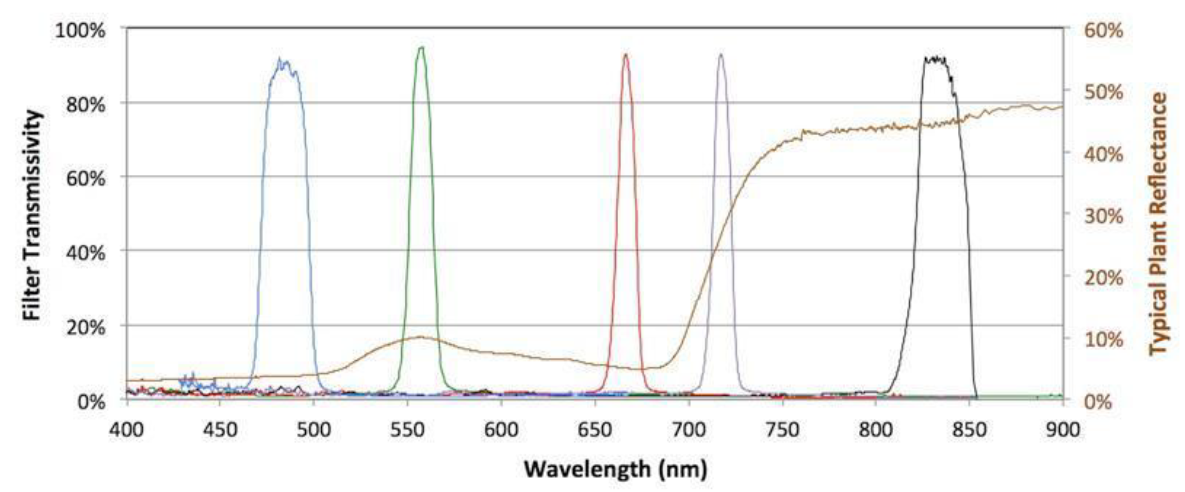
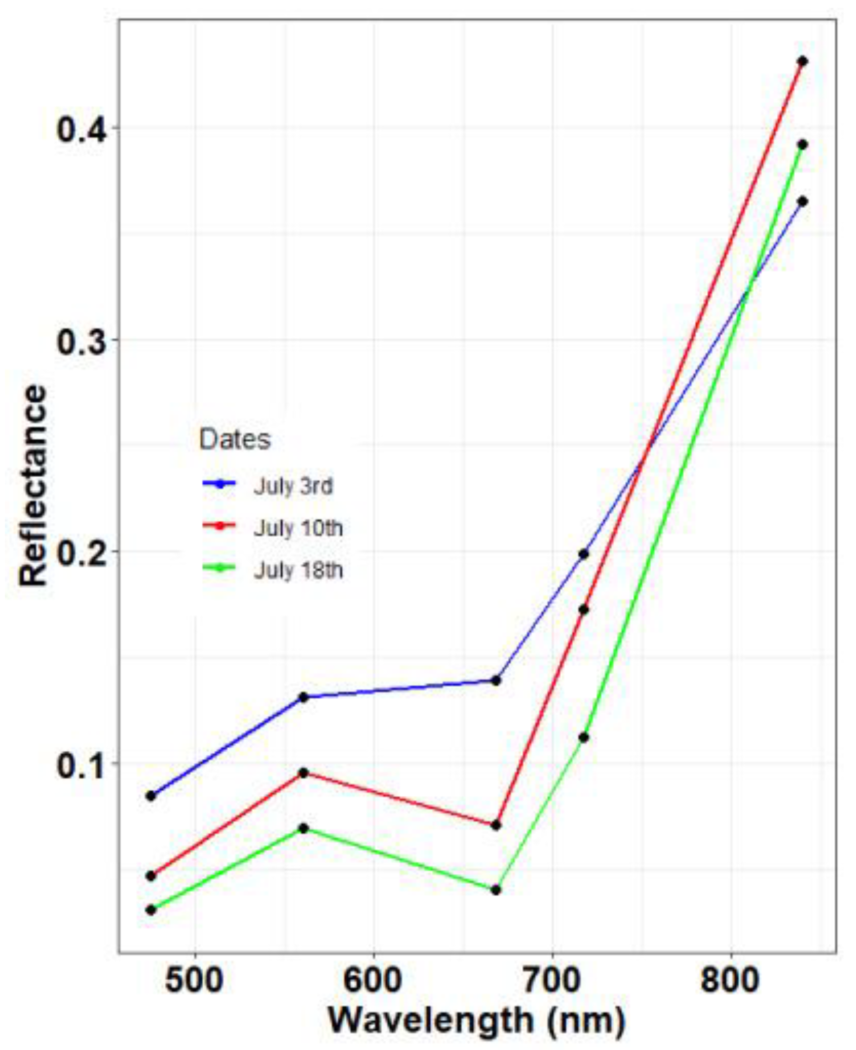
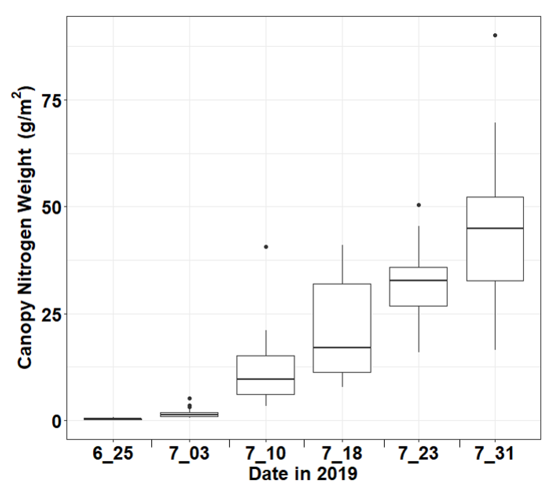
Our study used five different MicaSense multispectral bands to derive various VIs to predict canopy nitrogen weight. Values of the in-situ canopy nitrogen weight saw an increase in variation on 10 July and 18 July. This is due to the rapid increase in biomass between the dates. This could be explained by the crop biomass variation increasing due to the factors that contribute to the crop’s growth, such as the absorption, utilization, and transformation of solar energy; climate; and nutrient/water management [69,70].
Individual bands were tested to predict canopy nitrogen in all the models along with the VIs. Both the MicaSense green band and red-edge band performed poorly in the model compared to the other bands. The green wavelength is closely related to the leaf chlorophyll a and b contents (Zhao et al. [71]) in which nitrogen is used for plant photosynthesis. The poor performance in the model may be due to the chlorophyll saturating in the middle to the late growth stages, causing the crops to reflect the same amount of green wavelength. However, our results are not in agreement with Schlemmer et al. [72] and Li et al. [73], who observed a good relationship between the green reflectance and corn nitrogen weight. The red-edge spectral region is an interesting region, in which the position of the sharp change in reflectance (known as the red-edge position) is particularly known to be a sensitive indicator of leaf chlorophyll content [74,75,76]. The red-edge position changes in the wavelength of 680–800 nm depending on the strength of the absorption of chlorophyll [77]. Therefore, the narrowband of 10nm in the MicaSense red-edge band may have not fully captured the red-edge position throughout the growing season, whereas another sensor with different band ranges could have captured it. A possible consideration in the future would be to fly two cameras simultaneously and compare the results. Furthermore, the red-edge reflectance has been also found to be significantly related to corn nitrogen weight in Schlemmer et al. [72] and Li et al. [73]. Such difference in both green and red-edge reflectance can be explained by the fact that their study focused more on predicting nitrogen at individual growth stages, while our study considered all the growth stages in the model. All the top six VIs in the variable importance table use the near-infrared and red bands, indicating that they are both critical to the prediction of nitrogen. This is probably due to the chlorophyll absorption present in the red region and high reflectance of near-infrared energy for leaf development of healthy vegetation. However, the near-infrared band alone does not have a good relationship with canopy nitrogen weight, and therefore it must be included with other bands under the form of VIs. Interestingly, NDVI (the most commonly used VI in literature) did not perform as well as the top VIs in the variable importance plot. This is because NDVI is known to saturate with canopy nitrogen weight once the canopy of the crop becomes dense [32].
The use of the variable importance plot in Random Forests to eliminate spectral variable inputs was also performed in Osco et al. [28] on predicting canopy nitrogen in citrus trees. The authors used the top five and ten variables of 33 spectral variables and found there was a slight decrease in the model performance. Similar to our results, Osco et al. [28] found a decrease in performance relatively small, and the trade-off between the number of spectral indices used and obtained accuracy is something that should be considered. However, Osco et al. [28] used a different list of VIs, but the application of the variable importance plot was the same. Random Forests performed poorly on corn in Fan et al. [24] (R2 = 0.60) compared to partial least squares regression (R2 = 0.80) on the validation dataset. However, the authors used nitrogen content percentage at the leaf level and found weak correlation with most of the spectral variables, while our study incorporated our nitrogen values at the canopy level (g/m2). Random Forests with spectral variables on the validation set performed much better at the canopy level (R
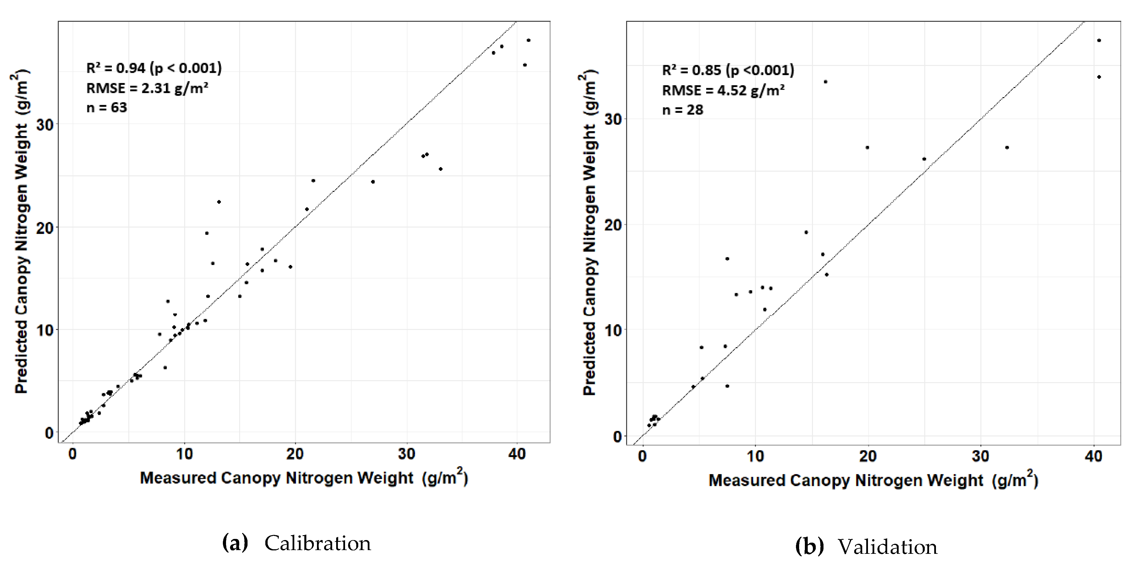
2 = 0.85), probably due to the spectral variables having a good correlation with nitrogen at the canopy level.
Our study on SVR modeling lines up with the results of Karimi et al. [31]. The authors found that SVR performed better and more consistent than its multiple linear regression counterpart in their study. The difference in results of Random Forests and SVR in our study are not too far apart in model performance. However, the concepts and outputs of Random Forests are a lot easier to interpret than the concepts and outputs of support vector machines.
Zha et al. [13] found Random Forests performed better than SVR, multiple linear regression and artificial neural networks on predicting nitrogen content in rice using spectral indices. A model comparison study using spectral indices in Liu et al. [3] also found Random Forests to perform better than the other non-parametric machine learning models in wheat. This could mean that the performance of Random Forests on nitrogen using spectral indices could be consistent on other types of crops and possibly give consistent results in different regions of Canada. Since different regions provide different climates, a comparison of the soil and nitrogen status in the crops could be studied. A consideration of future study could involve comparing Random Forests to other machine learning models or deep learning using spectral indices on other types of crops. However, delving into deep learning requires a huge training dataset in order to be effective. Another drawback is the computational cost such as memory and processing power in order to tackle the datasets effectively with deep learning.

5. Conclusions

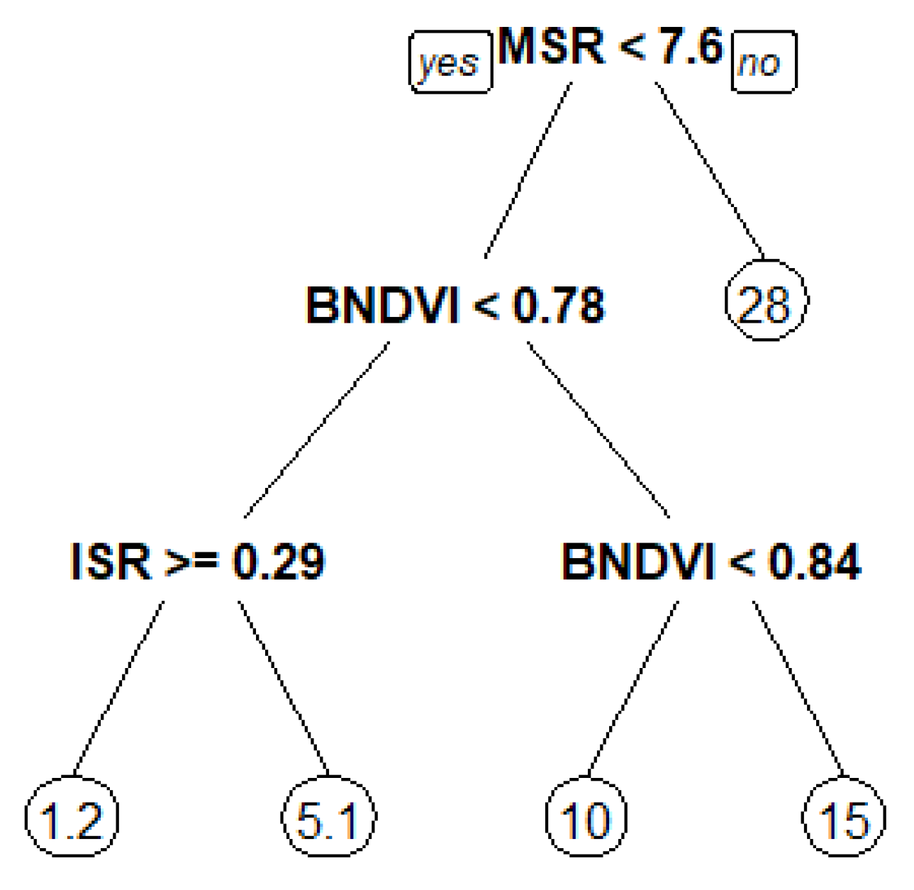
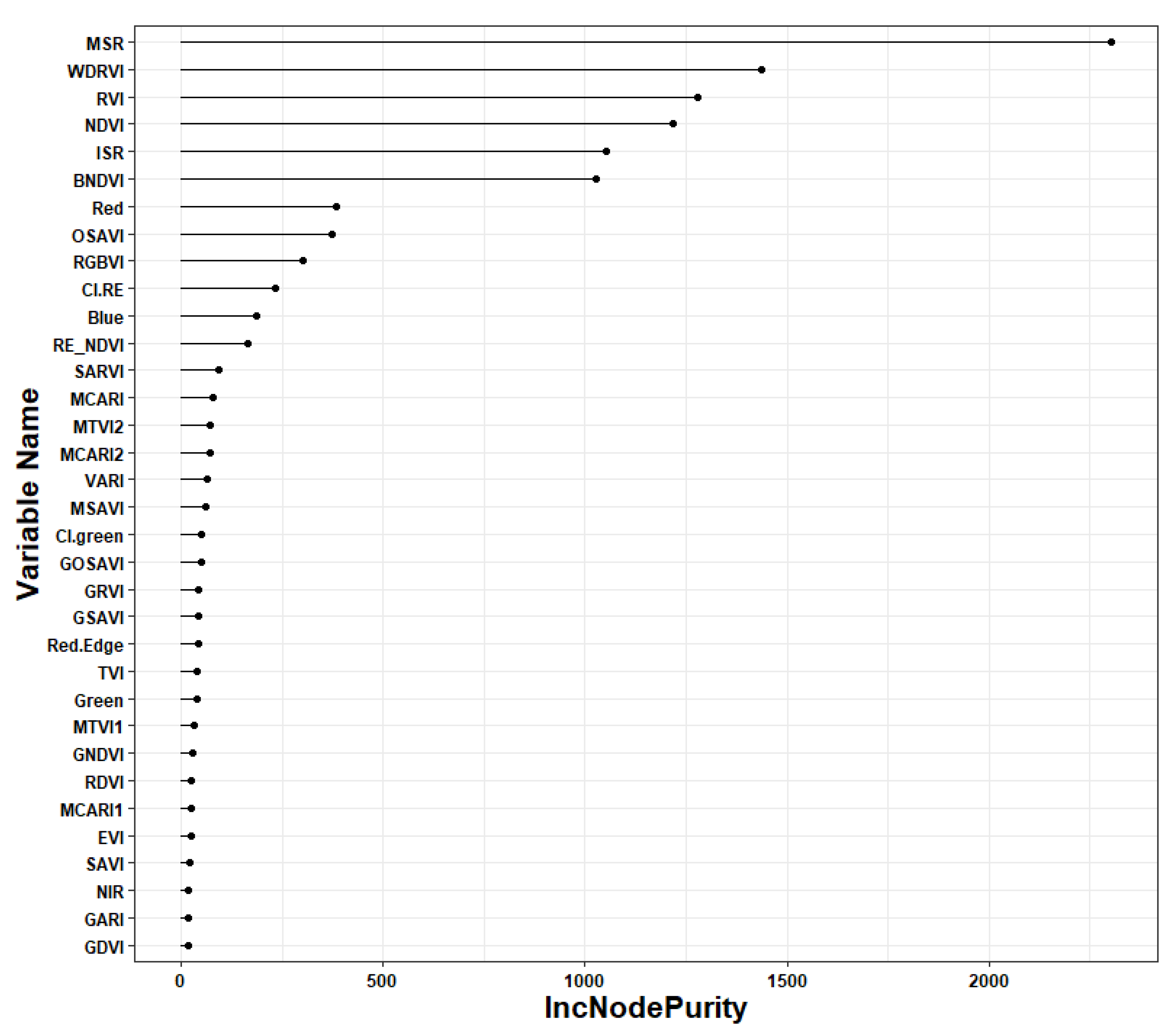
In this study, different regression methods were used to predict canopy nitrogen weight of corn using UAV MicaSense multispectral images. These models were established using the individual MicaSense bands and their associated VIs derived from the UAV reflectance values. Using the top 12 variables (in order: MSR, WDRVI, RVI, NDVI, ISR, BNDVI, Red band, OSAVI, RGBVI, CI Red edge, Blue band, and Red edge NDVI) derived with the Random Forests, the importance plot performed the best on estimating canopy nitrogen weight throughout the three dates in corn crops. Using the Random Forests model applied to the top 12 variables (RMSE = 4.52 g/m2) on the validation performed marginally worse than the Random Forests model using all the variables (RMSE = 4.51 g/m2), indicating that adding more variables into the model does not always improve its accuracy. However, because the difference of the accuracy is marginally different, this removes the unnecessary processing time of generating the 22 other VI images.
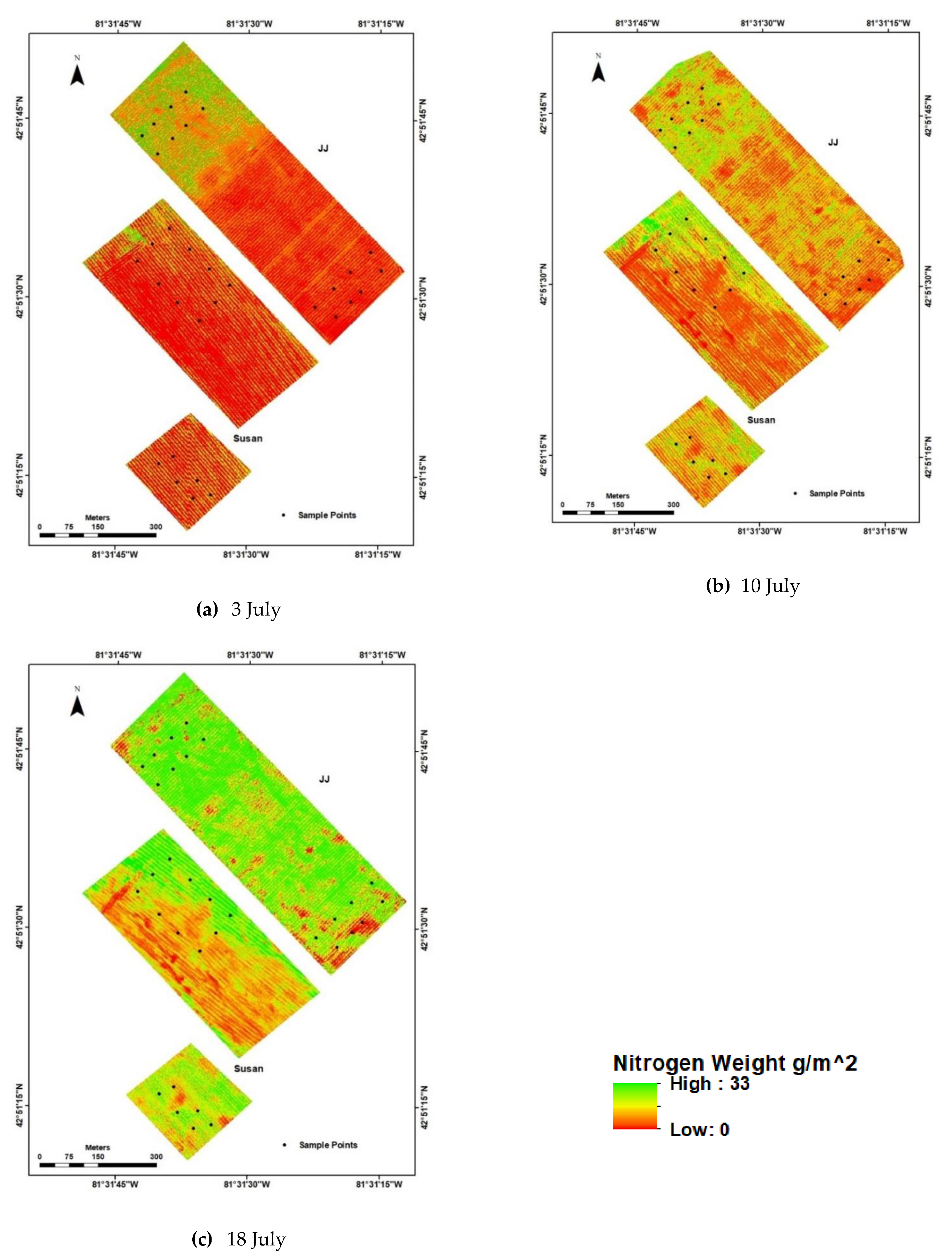
The UAV nitrogen prediction map can also detect spatial nitrogen variations within the field, especially in the 18 July image where the canopy nitrogen weight showed a large variation with the field data. In practice, these results could be useful for farmers in retrieving fast information about a field’s nitrogen status, as they will know exactly which parts of their fields are in excess or deficient in the amount of nitrogen present. Practically, these results could be obtained on the day of the UAV flight, depending on the size of the field and the number of images acquired. Ultimately, this will lead to a much more efficient fertilizer application program for the farmers as they will know precisely how much nitrogen is needed in a particular spot with their GPS-enabled fertilizer spreader.
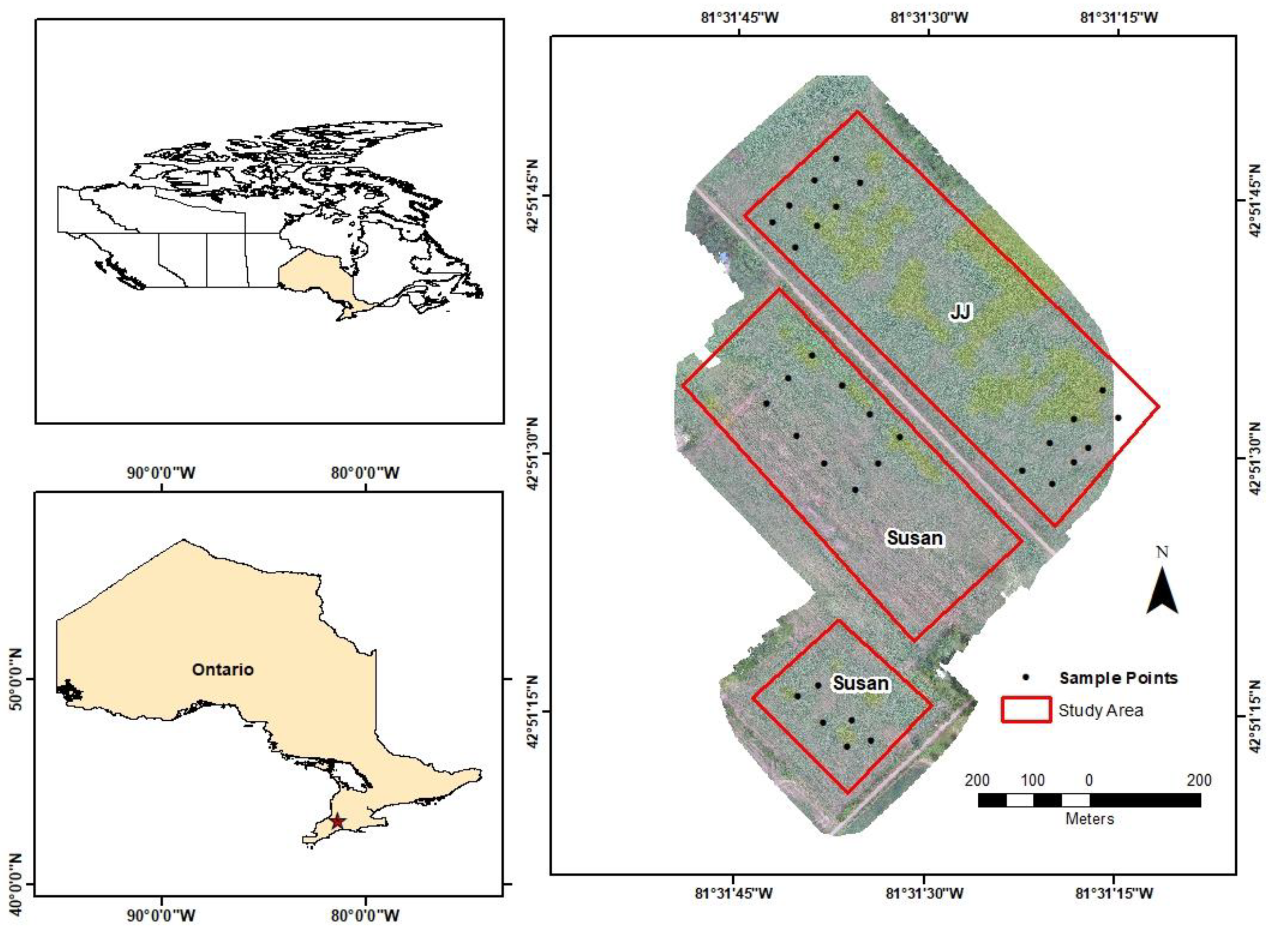
This study used data acquired over southwest Ontario fields in 2019 and there is the need to test the method over other datasets, such as different zones in Canada or a different crop. This will give an idea of how the developed method can be generalized and applied to different parts of Canada and whether it can be used on different crops. The study used MicaSense images with five spectral bands and there is a need to test different cameras that capture different wavelengths to understand which multispectral bands perform the best on predicting nitrogen using empirical regression techniques. Finally, another future consideration of this study can involve comparing the canopy nitrogen prediction map with other field spatial information, such as drainage and soil. This information can give a better idea on the contributions of nitrogen content that occur below the canopy.

Author Contributions

Conceptualization, H.L., J.W. and B.L.; methodology, H.L., J.F. and B.L.; software, H.L.; validation, J.W. and B.L.; formal analysis, H.L.; investigation, H.L.; resources, J.W. and B.L.; data curation, H.L.; writing—original draft preparation, H.L.; writing—review and editing, H.L., J.W. and B.L.; visualization, H.L.; supervision, J.W. and B.L.; project administration, B.L.; funding acquisition, B.L. and J.W. All authors have read and agreed to the published version of the manuscript.

Funding

This research is funded by an NSERC CRD grant number CRDPJ507141-16 awarded to Dr. Leblon and Dr. Wang and is the result of a collaboration between University of New Brunswick, University of Western Ontario, and A&L Canada Laboratories Inc.

Acknowledgments

The authors thank the A&L Canada Laboratories Inc staff and Dr. Wang’s GITA lab members for assistance with the fieldwork, lab processing, and UAV data collection. Special thanks go to Jody Yu, Robin Kwik, Gordon Cheung, Chunhua Liao, Steven McCreanor, Bo Shan, Hodan Holane, Daniel Kpienbaareh and Yang Song for their assistance in fieldwork and UAV data collection. The authors would also like to thank the anonymous reviewers for their helpful comments and feedbacks to this manuscript.

Conflicts of Interest

The authors declare no conflict of interest.

References

  1. Le Maire, G.; Francois, C.; Dufrene, E. Towards universal broad leaf chlorophyll indices using PROSPECT simulated database and hyperspectral reflectance measurements. Remote Sens. Environ. 2004, 89, 1–28. [Google Scholar] [CrossRef]
  2. Xie, Q.; Dash, J.; Huang, W.; Peng, D.; Qin, Q.; Mortimer, H.; Casa, R.; Pignatti, S.; Laneve, G.; Pascucci, S.; et al. Vegetation indices combining the red and red-edge spectral information for leaf area index retrieval. IEEE J. Sel. Top. Appl. Earth Obs. Remote Sens. 2018, 11, 1482–1493. [Google Scholar] [CrossRef] [Green Version]
  3. Liu, Y.; Cheng, T.; Zhu, Y.; Tian, Y.; Cao, W.; Yao, X.; Wang, N. Comparative analysis of vegetation indices, non-parametric and physical retrieval methods for monitoring nitrogen in wheat using UAV-based multispectral imagery. In Proceedings of the IEEE Internacional Geoscience and Remote Sensing Symposium (IGARSS), Beijing, China, 10–15 July 2016; pp. 7362–7365. [Google Scholar] [CrossRef]
  4. Shahhosseini, M.; Martinez-Feria, R.A.; Hu, G.; Archontoulis, S.V. Maize yield and nitrate loss prediction with machine learning algorithms. Environ. Res. Lett. 2019, 14, 124026. [Google Scholar] [CrossRef] [Green Version]
  5. Raparelli, E.; Bajocco, S. A bibliometric analysis on the use of unmanned aerial vehicles in agricultural and forestry studies. Int. J. Remote Sens. 2019, 40, 9070–9083. [Google Scholar] [CrossRef]
  6. Zheng, H.; Li, W.; Jiang, J.; Liu, Y.; Cheng, T.; Tian, Y.; Zhu, Y.; Cao, W.; Zhang, Y.; Yao, X. A comparative assessment of different modeling algorithms for estimating leaf nitrogen content in winter wheat using multispectral images from an unmanned aerial vehicle. Remote Sens. 2018, 10, 2026. [Google Scholar] [CrossRef] [Green Version]
  7. Zhang, C.; Kovacs, J.M. The application of small unmanned aerial systems for precision agriculture: A review. Precis. Agric. 2012, 13, 693–712. [Google Scholar] [CrossRef]
  8. Nasrallah, A.; Baghdadi, N.; Hajj, M.E.; Darwish, T.; Belhouchette, H.; Faour, G.; Darwich, S.; Mhawej, M. Sentinel-1 Data for Winter Wheat Phenology Monitoring and Mapping. Remote Sens. 2019, 11, 2228. [Google Scholar] [CrossRef] [Green Version]
  9. Bagheri, N.; Ahmadi, H.; Alavipanah, S.K.; Omid, M. Multispectral Remote Sensing for Site-Specific Nitrogen Fertilizer Management. Pesquisa Agropecuária Brasileira 2013, 48, 1394–1401. [Google Scholar] [CrossRef] [Green Version]
  10. Kelcey, J.; Lucieer, A. Sensor correction of a 6-band multispectral imaging sensor for UAV remote sensing. Remote Sens. 2012, 4, 1462–1493. [Google Scholar] [CrossRef] [Green Version]
  11. Yang, G.; Liu, J.; Zhao, C.; Li, Z.; Huang, Y.; Yu, H.; Xu, B.; Yang, X.; Zhu, D.; Zhang, X.; et al. Unmanned aerial vehicle remote sensing for field-based crop phenotyping:Current status and perspectives. Front. Plant Sci. 2017, 8, 1111. [Google Scholar] [CrossRef] [PubMed]
  12. Maresma, Á.; Ariza, M.; Martínez, E.; Lloveras, J.; Martínez-Casasnovas, J. Analysis of vegetation indices to determine nitrogen application and yield prediction in maize (Zea Mays, L.) from a standard UAV service. Remote Sens. 2016, 8, 973. [Google Scholar] [CrossRef] [Green Version]
  13. Zha, H.; Miao, Y.; Wang, T.; Li, Y.; Zhang, J.; Sun, W.; Feng, Z.; Kusnierek, K. Improving unmanned aerial vehicle remote sensing-based rice nitrogen nutrition index prediction with machine learning. Remote Sens. 2020, 12, 215. [Google Scholar] [CrossRef] [Green Version]
  14. Turner, D.; Lucieer, A.; Wallace, L. Direct georeferencing of ultrahigh-resolution UAV imagery. IEEE Trans. Geosci. Remote Sens. 2013, 52, 2738–2745. [Google Scholar] [CrossRef]
  15. Harwin, S.; Lucieer, A. Assessing the Accuracy of Georeferenced Point Clouds Produced via Multi-View Stereopsis from Unmanned Aerial Vehicle (UAV) Imagery. Remote Sens. 2012, 4, 1573–1599. [Google Scholar] [CrossRef] [Green Version]
  16. Clevers, J.G.P.W.; Kooistra, L. Using hyperspectral remote sensing data for retrieving total canopy chlorophyll and nitrogen content. IEEE J. Sel. Top. Appl. Earth Obs. Remote Sens. 2011, 5, 574–583. [Google Scholar] [CrossRef]
  17. Clevers, J.; Gitelson, A. Remote estimation of crop and grass chlorophyll and nitrogen content using red-edge bands on Sentinel-2 and-3. Int. J. Appl. Earth Obs. Geoinf. 2013, 23, 344–351. [Google Scholar] [CrossRef]
  18. Hansen, P.; Schjoerring, J. Reflectance measurement of canopy biomass and nitrogen status in wheat crops using normalized difference vegetation indices and partial least squares regression. Remote Sens. Environ. 2003, 86, 542–553. [Google Scholar] [CrossRef]
  19. Botha, E.J.; Leblon, B.; Zebarth, B.J.; Watmough, J. Non-destructive estimation of wheat leaf chlorophyll content from hyperspectral measurements through analytical model inversion. Int. J. Remote Sens. 2010, 31, 1679–1697. [Google Scholar] [CrossRef]
  20. Jay, S.; Maupas, F.; Bendoula, R.; Gorretta, N. Retrieving LAI, chlorophyll and nitrogen contents in sugar beet crops from multi-angular optical remote sensing: Comparison of vegetation indices and PROSAIL inversion for field phenotyping. Field Crop. Res. 2017, 210, 33–46. [Google Scholar] [CrossRef] [Green Version]
  21. Chen, P.; Haboudane, D.; Tremblay, N.; Wang, J.; Vigneault, P.; Li, B. New Spectral Indicator Assessing the Efficiency of Crop Nitrogen Treatment in Corn and Wheat. Remote Sens. Environ. 2010, 114, 1987–1997. [Google Scholar] [CrossRef]
  22. Tian, Y.; Yao, X.; Yang, J.; Cao, W.; Hannaway, D.; Zhu, Y. Assessing Newly Developed and Published Vegetation Indices for Estimating Rice Leaf Nitrogen Concentration with Ground-and Space-Based Hyperspectral Reflectance. Field Crop. Res. 2011, 120, 299–310. [Google Scholar] [CrossRef]
  23. Miphokasap, P.; Honda, K.; Vaiphasa, C.; Souris, M.; Nagai, M. Estimating canopy nitrogen concentration in sugarcane using field imaging spectroscopy. Remote Sens. 2012, 4, 1651–1670. [Google Scholar] [CrossRef] [Green Version]
  24. Fan, L.; Zhao, J.; Xu, X.; Liang, D.; Yang, G.; Feng, H.; Yang, H.; Chen, G.; Wei, P. Hyperspectral-based estimation of leaf nitrogen content in corn using optimal selection of multiple spectral variables. Sensors 2019, 19, 2898. [Google Scholar] [CrossRef] [PubMed] [Green Version]
  25. Li, F.; Gnyp, M.L.; Jia, L.; Miao, Y.; Yu, Z.; Koppe, W.; Bareth, G.; Chen, X.; Zhang, F. Estimating N status of winter wheat using a handheld spectrometer in the North China plain. Field Crop. Res. 2008, 106, 77–85. [Google Scholar] [CrossRef]
  26. Kayad, A.; Sozzi, M.; Gatto, S.; Marinello, F.; Pirotti, F. Monitoring within-field variability of corn yield using Sentinel-2 and machine learning techniques. Remote Sens. 2019, 11, 2873. [Google Scholar] [CrossRef] [Green Version]
  27. Belgiu, M.; Drăguţ, L. Random Forest in remote sensing: A review of applications and future directions. ISPRS J. Photogramm. Remote Sens. 2016, 114, 24–31. [Google Scholar] [CrossRef]
  28. Osco, L.P.; Ramos, A.P.M.; Pereira, D.R.; Moriya, É.A.S.; Imai, N.N.; Matsubara, E.T.; Estrabis, N.; Souza, M.D.; Junior, J.M.; Gonçalves, W.N.; et al. Predicting canopy nitrogen content in citrus-trees using Random Forest algorithm associated to spectral vegetation indices from UAV-Imagery. Remote Sens. 2019, 11, 2925. [Google Scholar] [CrossRef] [Green Version]
  29. Xiong, X.; Zhang, J.; Guo, D.; Chang, L.; Huang, D. Non-Invasive sensing of nitrogen in plant using digital images and machine learning for Brassica Campestris ssp. Chinensis L. Sensors 2019, 19, 2448. [Google Scholar] [CrossRef] [Green Version]
  30. Wang, L.; Zhou, X.; Zhu, X.; Guo, W. Estimation of leaf nitrogen concentration in wheat using the MK-SVR algorithm and satellite remote sensing data. Comput. Electron. Agric. 2017, 140, 327–337. [Google Scholar] [CrossRef]
  31. Karimi, Y.; Prasher, S.O.; Kim, S. Application of support vector machine technology for the estimation of crop biophysical parameters using aerial hyperspectral observations. Can. Biosyst. Eng. 2008, 50, 13–20. [Google Scholar]
  32. Lee, H.; Wang, J.; Leblon, B. Canopy nitrogen retrieval from unmanned aerial vehicle imagery for wheat and corn fields. Can. J. Remote Sens. 2020, accepted. [Google Scholar] [CrossRef]
  33. Deng, L.; Mao, Z.; Li, X.; Hu, Z.; Duan, F.; Yan, Y. UAV-based multispectral remote sensing for precision agriculture: A comparison between different cameras. ISPRS J. Photogramm. Remote Sens. 2018, 146, 124–136. [Google Scholar] [CrossRef]
  34. Ontario Farm Data. Ministry of Agriculture, Food and Rural Affairs 2017. Available online: http://www.omafra.gov.on.ca/english/stats/census/summary.htm (accessed on 18 June 2020).
  35. Frels, K.; Guttieri, M.; Joyce, B.; Leavitt, B.; Baenziger, P.S. Evaluating canopy spectral reflectance vegetation indices to estimate nitrogen use traits in hard winter wheat. Field Crop. Res. 2018, 217, 82–92. [Google Scholar] [CrossRef]
  36. AOAC Official Method 972.43. Microchemical determination of carbon, hydrogen, and nitrogen, automated method. Off. Methods Anal. AOAC Int. 2006, 12, 5–6. [Google Scholar]
  37. Pix4D Drone Mapping Software. Swiss Fed Inst Technol Lausanne, Route Cantonale, Switzerland 2014. Available online: http://pix4d.com (accessed on 1 June 2020).
  38. Tagle Casapia, M.X. Study of radiometric variations in Unmanned Aerial Vehicle remote sensing imagery for vegetation mapping. In Lund University GEM Thesis Series; Lund University Libraries: Lund, Switzerland, 2017. [Google Scholar]
  39. Wang, F.-M.; Huang, J.-F.; Tang, Y.-L.; Wang, X.-Z. New vegetation index and its application in estimating leaf area index of rice. Rice Sci. 2007, 14, 195–203. [Google Scholar] [CrossRef]
  40. Gitelson, A.A.; Yuri, G.; Merzlyak, M.N. Relationships between leaf chlorophyll content and spectral reflectance and algorithms for non-destructive chlorophyll assessment in higher plant leaves. J. Plant Physiol. 2003, 160, 271–282. [Google Scholar] [CrossRef]
  41. Huete, A.; Didan, K.; Miura, T.; Rodriguez, E.; Gao, X.; Ferreira, L. Overview of the radiometric and biophysical performance of the MODIS vegetation indices. Remote Sens. Environ. 2002, 83, 195–213. [Google Scholar] [CrossRef]
  42. Gitelson, A.A.; Merzlyak, M.N.; Lichtenthaler, H.K. Detection of red edge position and chlorophyll content by reflectance measurements near 700 nm. J. Plant. Physiol. 1996, 148, 501–508. [Google Scholar] [CrossRef]
  43. Tucker, C.; Elgin, J.; Mcmurtrey, J.; Fan, C. Monitoring corn and soybean crop development with hand-held radiometer spectral data. Remote Sens. Environ. 1979, 8, 237–248. [Google Scholar] [CrossRef]
  44. Gitelson, A.A.; Merzlyak, M.N. Remote sensing of chlorophyll concentration in higher plant leaves. Adv. Space Res. 1998, 22, 689–692. [Google Scholar] [CrossRef]
  45. Sripada, R.P. Determining In-Season Nitrogen Requirements for Corn Using Aerial Color-Infrared Photography. Ph.D. Thesis, North Carolina State University, Raleigh, NC, USA, 2005. [Google Scholar]
  46. Sripada, R.P.; Heiniger, R.W.; White, J.G.; Meijer, A.D. Aerial color infrared photography for determining early in-season nitrogen requirements in corn. Agron. J. 2006, 98, 968–977. [Google Scholar] [CrossRef]
  47. Fernandes, R.; Butson, C.; Leblanc, S.; Latifovic, R. Landsat-5 TM and Landsat-7 ETM+ based accuracy assessment of leaf area index products for Canada derived from SPOT-4 VEGETATION data. Can. J. Remote Sens. 2003, 29, 241–258. [Google Scholar] [CrossRef]
  48. Daughtry, C. Estimating corn leaf chlorophyll concentration from leaf and canopy reflectance. Remote Sens. Environ. 2000, 74, 229–239. [Google Scholar] [CrossRef]
  49. Haboudane, D. Hyperspectral vegetation indices and novel algorithms for predicting green LAI of crop canopies: Modeling and validation in the context of precision agriculture. Remote Sens. Environ. 2004, 90, 337–352. [Google Scholar] [CrossRef]
  50. Qi, J.; Chehbouni, A.; Huete, A.; Kerr, Y.; Sorooshian, S. A modified soil adjusted vegetation index. Remote Sens. Environ. 1994, 48, 119–126. [Google Scholar] [CrossRef]
  51. Chen, J.M. Evaluation of vegetation indices and a modified simple ratio for boreal applications. Can. J. Remote Sens. 1996, 22, 229–242. [Google Scholar] [CrossRef]
  52. Rouse, J.W.; Haas, R.H.; Schell, J.A.; Deering, D.W. Monitoring vegetation systems in the Great Plains with ERTS. NASA Spec. Publ. 1974, 351, 309. [Google Scholar]
  53. Rondeaux, G.; Steven, M.; Baret, F. Optimization of soil-adjusted vegetation indices. Remote Sens. Environ. 1996, 55, 95–107. [Google Scholar] [CrossRef]
  54. Roujean, J.L.; Breon, F.M. Estimating PAR absorbed by vegetation from bidirectional reflectance measurements. Remote Sens. Environ. 1995, 51, 375–384. [Google Scholar] [CrossRef]
  55. Gitelson, A.; Merzlyak, M.N. Quantitative estimation of chlorophyll-a using reflectance spectra: Experiments with autumn chestnut and maple leaves. J. Photochem. Photobiol. B Biol. 1994, 22, 247–252. [Google Scholar] [CrossRef]
  56. Bendig, J.; Yu, K.; Aasen, H.; Bolten, A.; Bennertz, S.; Broscheit, J.; Gnyp, M.L.; Bareth, G. Combining UAV-based plant height from crop surface models, visible, and near infrared vegetation indices for biomass monitoring in barley. Int. J. Appl. Earth Obs. Geoinf. 2015, 39, 79–87. [Google Scholar] [CrossRef]
  57. Jordan, C.F. Derivation of leaf-area index from quality of light on the forest floor. Ecology 1969, 50, 663–666. [Google Scholar] [CrossRef]
  58. Huete, A. A soil-adjusted vegetation index (SAVI). Remote Sens. Environ. 1988, 25, 295–309. [Google Scholar] [CrossRef]
  59. Broge, N.; Leblanc, E. Comparing prediction power and stability of broadband and hyperspectral vegetation indices for estimation of green leaf area index and canopy chlorophyll density. Remote Sens. Environ. 2001, 76, 156–172. [Google Scholar] [CrossRef]
  60. Gitelson, A.A.; Kaufman, Y.J.; Stark, R.; Rundquist, D. Novel algorithms for remote estimation of vegetation fraction. Remote Sens. Environ. 2002, 80, 76–87. [Google Scholar] [CrossRef] [Green Version]
  61. Gitelson, A.A. Remote estimation of crop fractional vegetation cover: The use of noise equivalent as an indicator of performance of vegetation indices. Int. J. Remote Sens. 2013, 34, 6054–6066. [Google Scholar] [CrossRef]
  62. R Core Team. R: A Language and Environment for Statistical Computing; R Foundation for Statistical Computing: Vienna, Austria, 2019; Available online: https://www.r-project.org/index.html (accessed on 1 June 2020).
  63. James, G.; Witten, D.; Hastie, T.; Tibshirani, R. An Introduction to Statistical Learning: With Applications in R; Springer: New York, NY, USA, 2013; p. 18. [Google Scholar]
  64. Louppe, G. Understanding Random Forests. Ph.D. Thesis, Cornell University, Ithaca, NY, USA, 2014. [Google Scholar]
  65. Čeh, M.; Kilibarda, M.; Lisec, A.; Bajat, B. Estimating the performance of Random Forest versus multiple regression for predicting prices of the apartments. ISPRS Int. J. Geoinf. 2018, 7, 168. [Google Scholar] [CrossRef] [Green Version]
  66. Liaw, A.; Wiener, M. Classification and regression by Random Forest. R News 2002, 2, 18–22. [Google Scholar]
  67. Meyer, D.; Dimitriadou, E.; Hornik, K.; Weingessel, A.; Leisch, F. e1071: Misc Functions of the Department of Statistics, Probability Theory Group (Formerly: E1071), TU Wien, R package version 1.7-3; R Foundation for Statistical Computing: Vienna, Austria, 2018. [Google Scholar]
  68. Hijmans, R.J. Raster: Geographic Data Analysis and Modeling, R package version, 3.0-7; R Foundation for Statistical Computing: Vienna, Austria, 2019. [Google Scholar]
  69. Yue, J.; Yang, G.; Li, C.; Li, Z.; Wang, Y.; Feng, H.; Xu, B. Estimation of winter wheat above-ground biomass using unmanned aerial vehicle-based snapshot hyperspectral sensor and crop height improved models. Remote Sens. 2017, 9, 708. [Google Scholar] [CrossRef] [Green Version]
  70. Campos, I.; González-Gómez, L.; Villodre, J.; González-Piqueras, J.; Suyker, A.E.; Calera, A. Remote sensing-based crop biomass with water or light-driven crop growth models in wheat commercial fields. Field Crop. Res. 2018, 216, 175–188. [Google Scholar] [CrossRef]
  71. Zhao, B.; Duan, A.; Ata-Ul-Karim, S.T.; Liu, Z.; Chen, Z.; Gong, Z.; Zhang, J.; Xiao, J.; Liu, Z.; Qin, A.; et al. Exploring new spectral bands and vegetation indices for estimating nitrogen nutrition index of summer maize. Eur. J. Agron. 2018, 93, 113–125. [Google Scholar] [CrossRef]
  72. Schlemmer, M.; Gitelson, A.; Schepers, J.; Ferguson, R.; Peng, Y.; Shanahan, J.; Rundquist, D. Remote estimation of nitrogen and chlorophyll contents in maize at leaf and canopy levels. Int. J. Appl. Earth Obs. Geoinf. 2013, 25, 47–54. [Google Scholar] [CrossRef] [Green Version]
  73. Li, F.; Miao, Y.; Feng, G.; Yuan, F.; Yue, S.; Gao, X.; Liu, Y.; Liu, B.; Ustin, S.L.; Chen, X. Improving estimation of summer maize nitrogen status with red edge-based spectral vegetation indices. Field Crop. Res. 2014, 157, 111–123. [Google Scholar] [CrossRef]
  74. Jones, H.G.; Vaughan, R.A. Remote Sensing of Vegetation: Principles, Techniques, and Applications; Oxford University Press: Oxford, UK, 2010. [Google Scholar]
  75. Zarco-Tejada, P.J.; Miller, J.R.; Mohammed, G.H.; Noland, T.L.; Sampson, P.H. Vegetation stress detection through chlorophyll a + b estimation and fluorescence effects on hyperspectral imagery. J. Environ. Qual. 2002, 31, 1433–1441. [Google Scholar] [CrossRef]
  76. Curran, P.J.; Dungan, J.L.; Gholz, H.L. Exploring the relationship between reflectance red edge and chlorophyll content in slash pine. Tree Physiol. 1990, 7, 33–48. [Google Scholar] [CrossRef]
  77. Baranoski, G.V.G.; Rokne, J.G. A practical approach for estimating the red edge position of plant leaf reflectance. Int. J. Remote Sens. 2005, 26, 503–521. [Google Scholar] [CrossRef]
Figure 1. Study area of the corn fields (JJ and Susan) shown using red green blue (RGB) sensor mosaic imagery taken on 18 July 2019 in Southwest Ontario, Canada. One corner of JJ is missing on the RGB image.
Remotesensing 12 02071 g001
Figure 2. Ground photos of corn (2019) taken on 26 June (left) and 31 July (right).
Remotesensing 12 02071 g002
Figure 3. Flowchart of the methodology.
Remotesensing 12 02071 g003
Figure 4. Spectral response curve for the MicaSense RedEdge Camera. The brown line is a typical reflectance profile of a green vegetation canopy. Figure derived from Tagle Casapia [38].
Remotesensing 12 02071 g004
Figure 5. An example of a generalized decision tree model in Random Forests (R Studio) using all the spectral variables.
Remotesensing 12 02071 g005
Figure 6. Spectral profile of the MicaSense reflectance using the center wavelength for each band.
Remotesensing 12 02071 g006
Figure 7. Box plot showing the variation of canopy nitrogen weight (g/m2) as a function of the date of field measurements in JJ and Susan corn field during the 2019 growing season. The dots on the graph represent outliers.
Remotesensing 12 02071 g007
Figure 8. Variance Importance plot using the function varImpPlot() in R Studio. Higher IncNodePurity values indicate more impact on nitrogen.
Remotesensing 12 02071 g008
Figure 9. Predicted versus measured canopy nitrogen weights when applying the Random Forests (RF) model to the top 12 variables for (a) the calibration dataset and (b) validation dataset.
Remotesensing 12 02071 g009
Figure 10. Canopy nitrogen prediction map derived when applying the RF model to the top 12 variable images for (a) 3 July, (b) 10 July, and (c) 18 July for the JJ and Susan fields. The locations of the ground sampling points are also given with a black dot.
Remotesensing 12 02071 g010
Table 1. Summary of Unmanned Aerial Vehicle (UAV) flight acquisition in the study (2019).
UAV Flight DateWeatherRelative HumidityCorn Growth Stage
26 June27 °C, Sunny69%V1/V2
3 July30.1 °C, Sunny58%V3/V4
10 July30.8 °C, Sunny45%V5
18 July29.3 °C, Sunny70%V6
23 July24.3 °C, Sunny73%V7/V8
31 July25.3 °C, Sunny60%V9
Table 2. Spectral characteristics of the five MicaSense bands.
Band #NameBand Range (nm)Center Wavelength (nm)Bandwidth (nm)
1Blue465–48547520
2Green550–57056020
3Red663–67366810
4Red edge712–72271710
5Near-infrared (NIR)820–86084040
Table 3. Vegetation indices used in the study.
Index (1)Formula (2)Authors
BNDVI(NIR − BLUE)/(NIR + BLUE)Wang et al. [39]
CI_Green(NIR/GREEN) − 1Gitelson et al. [40]
CI_RE(NIR/REDEDGE) − 1Gitelson et al. [40]
EVI 2.5 ( NIR RED ) ( NIR + 6 RED 7.5 BLUE ) + 1 Huete et al. [41]
GARI NIR - [ GREEN - 1.7 ( BLUE - RED ) ] NIR + [ GREEN 1.7 ( BLUE RED )   Gitelson et al. [42]
GDVINIR − GREENTucker et al. [43]
GNDVI( NIR - GREEN )/( NIR + GREEN )Gitelson; Merzlyak, [44]
GOSAVI(NIR − GREEN)/(NIR + GREEN + 0.16)Sripada et al. [45]
GRVI(GREEN − RED)/(GREEN + RED)Sripada et al. [46]
GSAVI1.5[(NIR − GREEN)/NIR + GREEN + 0.5)]Sripada et al. [45]
ISRRED/NIRFernandes et al. [47]
MCARI[(REDEDGE − RED) − 0.2(REDEDGE − GREEN)] *(REDEDGE/RED)Daughtry et al. [48]
MCARI11.2[2.5(NIR − RED) − 1.3(NIR − GREEN)]Haboudane et al. [49]
MCARI2   3.75 ( NIR RED ) 1.95 ( NIR GREEN ) ( 2 NIR + 1 2 ) ( 6 NIR 5 RED ) 0.5 Haboudane et al. [49]
MSAVI 2 NIR + 1 ( 2 NIR + 1 ) 2 8 ( NIR RED ) 2 Qi et al. [50]
MSR ( NIR / RED ) - 1 ( NIR RED ) + 1 Chen, [51]
MTVI11.2[1.2(NIR − GREEN) − 2.5(RED − GREEN)Haboudane et al. [49]
MTVI2 1.8 ( NIR - GREEN ) - 3.75 ( RED - GREEN ) ( 2 NIR + 1 ) 2 6 ( NIR 5 RED ) 0.5 Haboudane et al. [49]
NDVI(NIR − RED)/(NIR + RED)Rouse et al. [52]
OSAVI1.6[(NIR − RED)/(NIR + RED + 0.16)]Rondeaux; Steven; Baret, [53]
RDVI ( NIR - RED ) ( NIR + RED ) Roujean; Breon, [54]
RE_NDVI(NIR − REDEDGE)/(NIR + REDEDGE)Gitelson; Merzyak, [55]
RGBVI(GREEN2 − BLUE * RED)/(GREEN2 + BLUE * RED)Bendig et al. [56]
RVINIR/REDJordan, [57]
SARVI ( 1 + 0.5 ) ( NIR - y ) ( NIR + y + 0.5 ) Rondeaux; Steven; Baret, [53]
SAVI(NIR − RED)(1 + 0.5)/(NIR + RED + 0.5)Huete, [58]
TVI 120 ( NIR GREEN ) 200 ( RED GREEN ) 2 Broge; Leblanc, [59]
VARI(GREEN − RED)/(GREEN + RED − BLUE)Gitelson et al. [60]
WDRVI(0.2 * NIR − RED)/(0.2 * NIR + RED)Gitelson, [61]
1 BNDVI = blue normalized difference vegetation index; CI_Green = chlorophyll index green; CI_RE = chlorophyll index red edge; EVI = enhanced vegetation index; GARI = green atmospherically resistant index; GDVI = green difference vegetation index; GNDVI = green normalized difference vegetation index; GOSAVI = green optimized soil adjusted vegetation index; GRVI = green ratio vegetation index; GSAVI = green soil adjusted vegetation index; ISR = infrared simple ratio; MCARI = modified chlorophyll absorption ratio index; MSAVI = modified soil adjusted vegetation index; MSR = modified simple ratio; MTVI = modified triangular vegetation index; NDVI = normalized difference vegetation index; OSAVI = optimized soil adjusted vegetation index; RDVI = renormalized difference vegetation index; RE_NDVI = red edge normalized difference vegetation index; RGBVI = red green blue vegetation index; RVI = ratio vegetation index; SARVI = soil atmospherically resistant vegetation index; SAVI = soil adjusted vegetation index; TVI = triangular vegetation index; VARI = visible atmospherically resistant index; WDRVI = wide dynamic range vegetation index; 2 BLUE = blue reflectance; GREEN = green reflectance; RED = red reflectance; REDEDGE = red edge reflectance; NIR = near-infrared reflectance; y = (RED − 1) * (BLUE − RED).
Table 4. Summary statistics of calibration and validation set for leaf nitrogen content%.
Calibration SetValidation Set
DateGrowth StageMin.Max.AverageMin.Max.Average
3 JulyV3/V43.975.935.154.396.155.41
10 JulyV52.574.513.612.294.293.48
18 JulyV62.244.053.642.974.313.60
Table 5. Summary statistics of calibration and validation set for dry biomass (g/m2).
Calibration SetValidation Set
DateGrowth StageMin.Max.AverageMin.Max.Average
3 JulyV3/V42.314.275.311.2919.74.64
10 JulyV523.8140.350.7521.475.1137.63
18 JulyV630.0210.689.3235.0148.980.9
Table 6. Statistics for the calibration of the canopy nitrogen model using various modeling approaches (n = 63) 1.
Input VariablesNumber of VariablesModelRMSE (g/m2)R2
All VIs and 5 MicaSense bands34RF2.250.95
MSR, WDRVI, RVI, NDVI, ISR, BNDVI, Red 2, OSAVI, RGBVI, CI_RE, Blue 2, RE_NDVI12RF2.310.94
MSR, ISR, RVI, NDVI, BNDVI, WDRVI6RF2.630.93
MSR, WDRVI, RVI, NDVI, ISR, BNDVI, Red 2, OSAVI, RGBVI, CI_RE, Blue 2, RE_NDVI12SVR3.980.87
12Linear4.030.87
All VIs and 5 MicaSense bands34SVR4.080.87
MSR, ISR, RVI, NDVI, BNDVI, WDRVI6Linear4.200.85
6SVR4.280.85
MSR1Linear4.410.83
All VIs and 5 MicaSense bands34Linear9.140.58
1 All models are significant at p-value < 0.001; 2 MicaSense individual band. RMSE, Root Mean Square Error.
Table 7. Statistics when applying various modeling approaches to the validation dataset (n = 28) 1.
Input VariablesNumber of VariablesModelRMSE (g/m2)R2
All VIs and 5 MicaSense bands34RF4.510.85
MSR, WDRVI, RVI, NDVI, ISR, BNDVI, Red 2 OSAVI, RGBVI, CI_RE, Blue 2, RE_NDVI12RF4.520.85
All VIs and 5 MicaSense bands34SVR4.580.84
MSR, WDRVI, RVI, NDVI, ISR, BNDVI, Red 2, OSAVI, RGBVI, CI_RE, Blue 2, RE_NDVI12SVR4.740.84
MSR, WDRVI, RVI, NDVI, ISR, BNDVI, Red 2, OSAVI, RGBVI, CI_RE, Blue 2, RE_NDVI12Linear4.780.85
MSR, ISR, RVI, NDVI, BNDVI, WDRVI6RF5.210.83
MSR1Linear 5.470.82
1 All models are significant at p-value < 0.001; 2 MicaSense individual band.

