Using Deep Learning to Count Albatrosses from Space: Assessing Results in Light of Ground Truth Uncertainty


1
School of Computing Sciences, University of East Anglia, Norwich NR4 7TJ, UK
2
Mapping and Geographic Information Centre, British Antarctic Survey, Cambridge CB3 0ET, UK
*
Author to whom correspondence should be addressed.
Remote Sens. 2020, 12(12), 2026; https://doi.org/10.3390/rs12122026
Submission received: 15 May 2020
/
Revised: 19 June 2020
/
Accepted: 21 June 2020
/
Published: 24 June 2020
Abstract
:Many wildlife species inhabit inaccessible environments, limiting researchers ability to conduct essential population surveys. Recently, very high resolution (sub-metre) satellite imagery has enabled remote monitoring of certain species directly from space; however, manual analysis of the imagery is time-consuming, expensive and subjective. State-of-the-art deep learning approaches can automate this process; however, often image datasets are small, and uncertainty in ground truth labels can affect supervised training schemes and the interpretation of errors. In this paper, we investigate these challenges by conducting both manual and automated counts of nesting Wandering Albatrosses on four separate islands, captured by the 31 cm resolution WorldView-3 sensor. We collect counts from six observers, and train a convolutional neural network (U-Net) using leave-one-island-out cross-validation and different combinations of ground truth labels. We show that (1) interobserver variation in manual counts is significant and differs between the four islands, (2) the small dataset can limit the networks ability to generalise to unseen imagery and (3) the choice of ground truth labels can have a significant impact on our assessment of network performance. Our final results show the network detects albatrosses as accurately as human observers for two of the islands, while in the other two misclassifications are largely caused by the presence of noise, cloud cover and habitat, which was not present in the training dataset. While the results show promise, we stress the importance of considering these factors for any study where data is limited and observer confidence is variable.
1. Introduction
Conducting regular wildlife surveys is essential for monitoring population health and informing conservation action [1,2]. Traditionally, such surveys have been conducted by direct human observation, where animals are physically counted from the ground, aerial platforms or boats. This can be an inexact science, prone to errors due to animals moving or being obscured from view, and additionally hindered by site accessibility, logistical costs and weather constraints, particularly in remote regions [3,4,5]. While the rapid uptake of new technology such as drones and camera traps has alleviated many of these issues [6,7], human operators are still required to visit field sites, which can limit their application in very inaccessible locations. In the last decade the advent of sub-metre Very High Resolution (VHR) satellite imagery has offered a new alternative—to survey wildlife directly from space [8]. In particular, VHR remote sensing has been increasingly employed to survey wildlife in remote areas, ranging from Wildebeest in African Savannah [9] to Polar Bears in the Arctic [10]. The additional benefits of large spatial coverage, minimal disturbance to wildlife and a permanent visual survey record means that VHR satellites could revolutionize monitoring practices for a range of species [8].
Despite the promise that VHR satellites hold, currently images must be manually analysed by experts, which hinders their application in practice. While researchers would benefit from surveying large areas (e.g., searching for whales in open ocean [4]), manually scanning through enormous volumes of imagery becomes a near impossible task, particularly if surveys are to be repeated regularly [11]. Due to this most research has been limited to comparatively small scale studies over a few square kilometers [2]. Challenges with manual analysis are exacerbated by the fact that wildlife is small and hard to distinguish. Even large animals appear as only a few pixels [12], and are generally only discernible due to a strong spectral contrast with their habitat, opposed to other recognisable features such as their shape and patterning [8]. If spectral reflectance values of the target animal overlap with non-target objects in the surrounding landscape, the two can be very difficult to differentiate [13]. This makes manual detection not only time-consuming but also highly subjective, with counts varying between annotators due to uncertainty [14]. This interobserver variation means that errors associated with counts can be hard to interpret. These factors strongly motivate the development of automated image processing algorithms, to improve speed, reduce cost and standardise the counting procedure [15].
When considering automated image analysis, methods can be broadly grouped into two categories—unsupervised and supervised classification. In unsupervised classification, statistical methods are used to automatically group pixels into clusters based on their spectral properties [2]. In contrast, supervised classification relies on users first annotating known objects in a dataset, then using these labelled examples to train a classifier. While unsupervised approaches are desirable as they require minimal user input, making them more standardised and theoretically easier to transfer across different datasets, in the vast majority of cases they are outperformed by supervised schemes. In particular, supervised deep learning algorithms have shown tremendous results in recent years, reaching state-of-the-art performance in tasks such as image classification and object detection. Convolutional neural networks (CNNs), a branch of deep learning classifiers inspired by the human vision system, have vastly improved our ability to detect objects in complex and noisy imagery [16]. A large part of their success can be attributed to the development of large scale labelled datasets, such as ImageNet [17], offering high quality annotated images at an unprecedented scale (over 14 million images covering 20 thousand object categories). Finding connections between image and label in these enormous and hugely varied datasets is how CNNs showed their true potential [18]. CNNs are now widely applied to a number of computer vision tasks, including detecting wildlife in drone [19], camera trap [20] and satellite [11] imagery.
Despite their proven success, there are challenges when using supervised CNNs to detect wildlife in satellite imagery. The first is that annotated datasets are small and costly to obtain. At present purchasing VHR satellite imagery over large extents can be expensive, and the added time and effort required for manual analysis has restricted many studies to one or two images [2,12]. However, deep learning algorithms perform best when supplied with a large and diverse set of training images, and without sufficient variation we can not be confident in the algorithms ability to generalize to new unseen data. While some researchers have found inventive ways of generating training data from other sources, such as downsampled aerial imagery [11], many studies consider only a single large satellite image which is divided up into smaller patches to train and test a classifier. Results from these methods are almost inevitably biased due to non-independence of the train and test patches, and we may see a significant drop in performance if an image with different characteristics is presented. The second challenge is with the labels used in our supervised training scheme, which as discussed are subject to interobserver variation and uncertainty. As in supervised training the accuracy of a classifier is limited by the accuracy of the provided labels, it is important to establish the level of uncertainty before evaluating performance. In the absence of a gold-standard ground truth (i.e., the direct linking of satellite data to concurrent ground based surveys) 100% accuracy cannot be the goal, and would in fact indicate overfitting to a single observer’s subjective annotations [21]. Only when we understand how accurately and consistently humans perform at the task, can we benchmark the performance of an automated approach.
In this paper, we wish to investigate the level of interobserver variation in manual counts, and study the effect of label choice on a supervised CNN classifier. We use the example of detecting Wandering Albatrosses Diomedea Exulans in 31 cm resolution WorldView-3 (WV-3) imagery as a test case. An automated method for detecting Wandering Albatrosses would be of great benefit, as the species nest almost exclusively on remote islands in the Southern Oceans, making ground based surveys challenging, expensive and infrequent (with gaps of up to 40 years between successive surveys) [22]. This is of particular concern given their listing as “vulnerable” under the IUCN Red List (IUCN 2020, iucnredlist.org), attributed to the impacts of long-line fishing, disease and the introduction of pests to their nesting habitats [23]. The species was first shown to be identifiable in WV-3 imagery in 2017 by Fretwell et al. [14], who validated their methods by comparing satellite counts to ground based observations (we refer the reader to this publication for further details on detectability and interpretation of satellite counts in relation to traditional sampling methods). This was the first example of using the WV-3 sensor to count birds directly, adding to previous works which surveyed birds using indirect VHR satellite observations (e.g., extrapolating numbers of Emperor [24], Adélie [25] and Chinstrap [26] penguins based on colony area, and using Google Earth satellite images to detect the nests of Masked Boobies [27]). While individual Wandering Albatrosses are directly detectable in WV-3 imagery the signature is weak (comprising of only several white pixels) and therefore subject to a large degree of uncertainty, making it a good candidate for investigating interobserver variation. Additional WV-3 imagery was also collected as part of a later study [22], leaving a comparatively large dataset of four separate islands, displaying differences in vegetation, cloud cover and lighting. A CNN has shown promising performance on the dataset already [28], but a greater understanding of interobserver variation is needed to place the results in context. With this in mind we aim to (1) assess the level of interobserver variation in manual counts for all images in the dataset (2) train a CNN using leave-one-island-out cross-validation, to consider how well the method generalises across images given the small dataset, and (3) consider the impact the choice of ground truth labels has in both training and evaluating the CNN. This represents the first automated method for detecting Wandering Albatrosses, or indeed any individual bird, in very high resolution satellite imagery.
2. Materials and Methods
2.1. Imagery
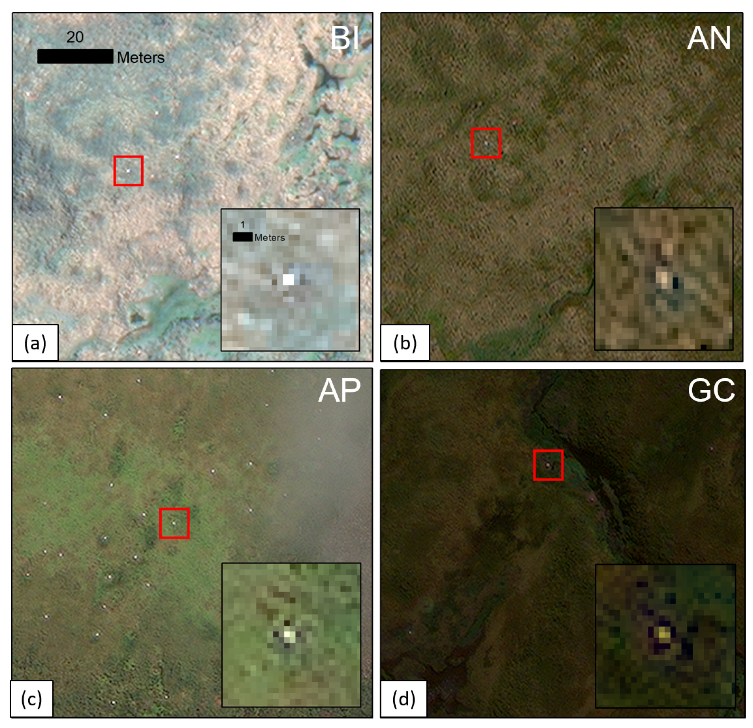
All satellite imagery was collected by the highest resolution commercially available sensor—DigitalGlobe’s WorldView-3 satellite. This samples at a spatial resolution of 31 cm per pixel in the panchromatic band, and 124 cm per pixel in the multispectral bands (in this study we use four multispectral bands; red, green, blue and near-infrared). As Wandering Albatrosses are largely white, with a body length of 107–135 cm [29], individuals appear as several pixels of white against their green nesting habitat (see Figure 1 and Supplementary Table S2 for examples). This is not greatly altered if a bird has extended wings due to darker feathers on the upper wing [14]. We collated images of four separate colonies of Wandering Albatrosses, originally collected as part of previous studies (namely, the works in [14,22]). The colonies are located on Bird Island (BI) and Annenkov Island (AN) in South Georgia, Apotres (AP) in the Crozet islands and Grande Coulee (GC) on the west coast of Kerguelen Island. Images were collected over different months and times of day, and present variation in terms of cloud cover, lighting and vegetation. They also differ in size, with the smallest (BI) covering 16 km2 and the largest (AN) covering 105 km2 (Supplementary Table S1).
2.2. Manual Counts
All four images had been annotated previously by the same experienced observer (we term these our “reference observer” annotations). To extend this and assess interobserver variation, we conducted additional labelling experiments with five novice volunteers (observer 1–5). For visual analysis the panchromatic and multispectral bands were pan-sharpened using the Gram–Schmidt algorithm (implemented in ArcMap software), resulting in a high resolution RGB image. These were viewed in ArcMap 10.5, with Figure 1 showing examples of the visual appearance of albatrosses in all four images.
We follow the annotation procedure outlined in the original study [14], whereby images were labelled by eye using separate polygons approximately matching the size of the monitor (in our case m for viewing at a 1:600 scale). To restrict changes in viewing conditions, we used the same monitor and controlled ambient lighting. Volunteers were given the same information prior to annotating, and identical image patches were used to present examples of albatrosses and potentially confounding features such as rocks. For our analysis we investigate how closely total observer counts match, the extent of overlap between annotations, and whether there is a best measure for combining them. This includes taking the union of all points (i.e., include any point labelled by an observer), the intersection (i.e., only include points labelled by all six observers) and each level in between (i.e., only include points labelled by at least two observers, at least three, etc.).
2.3. Detection Network
2.3.1. CNN overview
CNNs are generally structured as a series of layers, with the initial layers performing feature learning and final layers performing classification. The feature learning stage typically consists of alternate convolution and pooling operations, which sequentially transform the input image into higher level abstracted representations. For example, an initial layer may identify edges, the second may extract motifs from these edges, and a third may assemble these motifs into objects. The final classification stage is carried out by one or more fully connected layers and a classifer such as softmax. In CNNs, all weights and biases determining feature learning and classification are initialised randomly, and learned during training. The most common approach to training CNNs is through supervised training schemes, using backpropagation with gradient descent. In this method weights and biases are updated in order to minimise a loss function, which quantifies the difference between the output predicted by the network and the ground truth.
2.3.2. Network Architecture
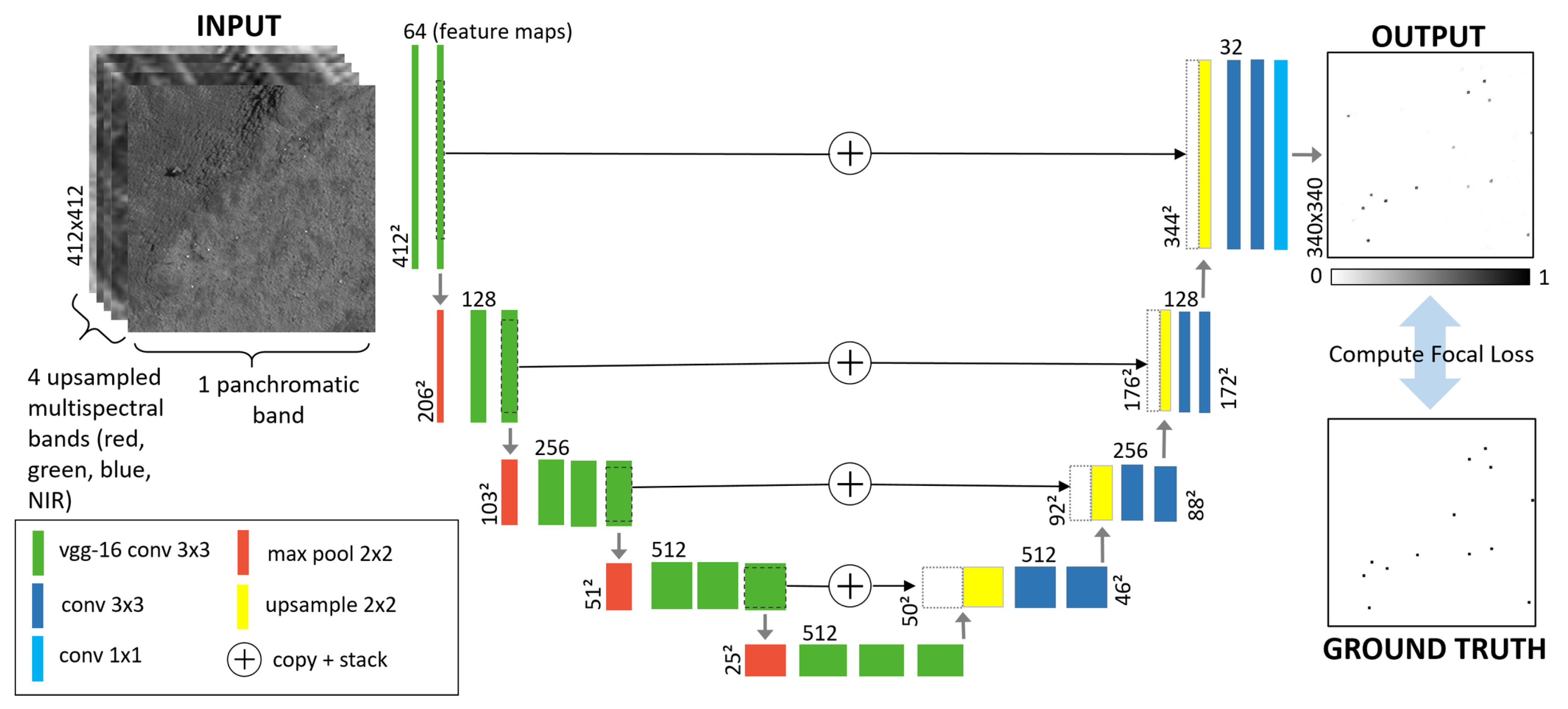
For our CNN we use a U-Net architecture, which was originally designed for biomedical image segmentation [30], but has recently shown state-of-the-art performance in a range of tasks. U-Net works by classifying every pixel in the image into a class (in our case albatross and non-albatross). The output probability map (Figure 2) can be directly overlaid with the input image, allowing us to classify and localize albatrosses in a single stage. We present the exact architecture in Figure 2, which closely follows that described in an earlier study [28]. The contracting path (left) follows the typical architecture of a CNN, applying repeated convolutions, ReLU activation, and max pooling to extract features from input images. The expanding path (right) upsamples feature maps and concatenates them with higher resolution information cropped and copied from the corresponding layer in the contracting path. This allows for precise localization of classified pixels.
Given our small dataset we use transfer learning, a method where convolution filters learned from a larger dataset are copied across to the new network. In principle these represent a generic set of filters, which can be used to extract low-level features common to all images (e.g., edges, patterns and gradients). We initialise our network using filters from a vgg-16 network [31], pre-trained on the ImageNet database [17]. To minimise information loss at the edge of images, we choose not to use padding in convolution operations (aside from those transferred from vgg-16), thus the output predictions are of reduced size ( compared to inputs). Experiments also showed no performance gain when using learnt upsampling (through upconvolution), so we favour bilinear upsampling for simplicity.
2.3.3. Dataset Processing
To train and test U-Net, we tiled all four satellite images into pixel square patches. The four multispectral bands (red, green, blue and near-infrared) were upsampled using bilinear interpolation to match the dimensions of the panchromatic image. ArcMap shapefiles generated by our six observers were converted into binary segmentation maps (with background = 0, albatross = 1), which were also tiled into patches exactly overlaying the input images. As the exact placement of observer labels can differ slightly, we use template matching [32] to shift observer annotations to the centre of each albatross. We segmented albatrosses using a pixel square, which was based on visual inspection of the imagery and matched the size of the majority of observer identified features.
To keep the dataset proportional we chose an equal number of patches from each island (500 patches from the land and 250 patches from the sea). These numbers approximately represent the maximum number of patches present in the smallest image (BI). For our leave-one-island-out cross-validation we trained the network on patches from three islands: resulting in 2250 patches in total, with 20% of these reserved for validation. Input patches of size , as well as their corresponding target patches of size , were cropped randomly from the larger tiles to augment the dataset. Tiles were also randomly flipped and reflected to add further variation. At test stage the fourth unseen image was tiled, and the trained network was run over all patches to generate a final prediction.
2.3.4. Training Parameters
As in our dataset the number of albatross pixels is vastly outweighed by background instances, there is a danger the network would favour ignoring all albatrosses to achieve a high accuracy on the more prevalent class. To account for this, we calculate the error between output and ground truth using the Focal Loss, proposed by the authors of [33], as a method for addressing extreme foreground background class imbalance [28]. It works by adding a modulating factor to the standard cross entropy criterion, which places more focus on hard, misclassified examples. If denotes the ground truth class and is the model’s estimated probability for the class with label , then the focal loss can be expressed as:
Increasing the focusing parameter reduces the loss contribution from easy to classify background examples. We ran experiments to assess the best choice for , and found that and gave the best results. We trained the model using the Adam optimizer, a learning rate of 0.0001 (degrading to 0.00001 after 5 epochs), and a mini-batch size of 4.
As we approach detection using a supervised training scheme, it is important to consider how the choice of ground truth will affect our results. This can happen at both the assessment stage (i.e., when comparing our network predictions against our chosen ground truth) and at the training stage (i.e., when choosing which labels to use when training our network). For our experiments at the assessment stage we use the majority vote labels (i.e., only points annotated by at least three observers are included in the ground truth) to train the network. The choice for this is detailed later in Section 3.1. We then assess the results of the network against all individual observers labels (the reference observer and observers 1–5), as well as the intersection, union, and majority vote. When assessing the impact of label noise at the training stage, we invert this and train on the different options for ground truth and assess using the majority vote. We also experiment with training using a “mixed” ground truth, where we select a random observers labels for every patch, at every epoch. We hypothesise that this random shuffling will automatically encode observer uncertainty, as points which are only labelled by one observer will appear on average one sixth of the time, whereas those with complete observer agreement will appear 100% of the time. For all analysis we train each individual model three times, and present the results as the average of all three, to mitigate for variation. All other network parameters are kept the same, only the ground truth labels are altered.
3. Results
To quantitatively evaluate results, we compare our network detections to ground truth labels. If the network detects an albatross, and it has also been labelled in the ground truth, it is marked as a true positive (TP). Misclassifications come in the form of false positives (FPs, i.e., the network detects an albatross but it is not labelled in the ground truth), and false negatives (FNs, i.e., the network does not detect an albatross which is labelled in the ground truth). Results are reported in terms of recall (the fraction of labelled albatrosses detected) and precision (the fraction of detections matching labelled albatrosses). To combine these as an overall accuracy we use the F1-score, the harmonic mean of recall and precision (Equation (2)) [32].
As our CNN outputs a probability map, the trade off between precision and recall can vary depending where we threshold the prediction. To assess results of the CNN we therefore calculate precision and recall for a range of threshold values and plot the results as a precision-recall curve [32]. We use the average precision (AvP, i.e., the area under the precision–recall curve) to evaluate and compare network results. Taking the average of these scores across all islands gives us the mean average precision (mAP).
3.1. Manual Counts
The variation in total counts between observers was significant in some cases, and also differed between the four images (Table 1). For example BI counts range from 612 to 994, with a deviation of 17% from the mean. In contrast AP shows significantly higher agreement in total counts, with a deviation of only 3% from the mean. This variation is likely to be due to the differences in both the appearance of albatrosses, and the number of other spectrally similar objects in the background. For example in Figure 1 we can see that albatrosses are much clearer in AP, with the white points strongly contrasting against the bright green, relatively uniform vegetation. In some cases albatrosses are also encircled by a brown ring, indicating a cleared area of vegetation surrounding the nest. However in other islands the contrast is weaker, with vegetation appearing more yellow (Figure 1a) and albatrosses not as bright (Figure 1b). This being said, it is important to note that total counts do not capture the agreement between labels (two observers could label 100 completely separate points), and to assess observer agreement we must compare how many annotations coincide with the same feature.
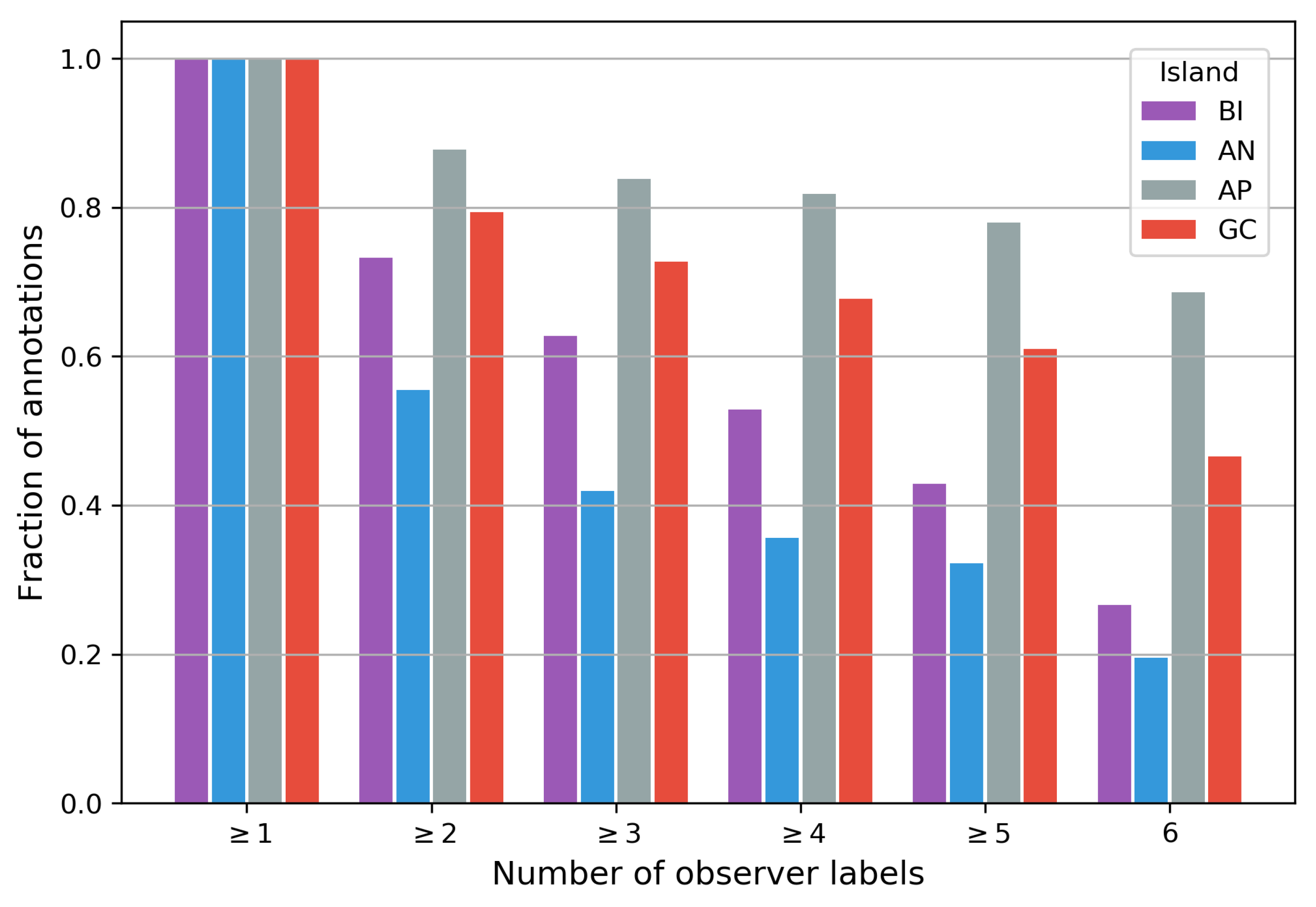
Figure 3 shows the fraction of identified features which were labelled by at least one observer (obviously 100%), at least two observers, at least three, etc. We see that for AP, over 84% of points in the image are labelled by at least three observers (i.e., the majority), suggesting strong agreement for a large fraction of the ground truth. GC shows a similarly high agreement with 73% of annotations having majority agreement. However, for AN there is a particularly steep drop, with only 42% of annotations agreed on by the majority, and over half the ground truth made up of low confidence annotations. This level of ground truth uncertainty is likely to have a noticeable impact on our supervised CNN.
In Table 2 we show the interobserver agreement for each of the four islands. For our analysis we take one observer’s labels as a predicted result, and assess the accuracy of their “predictions” against another observer’s ground truth (using the F1-score as our accuracy). Obviously when the same annotation is used we have an accuracy of 100%, the scores are also symmetric along the diagonal. Once again the overall agreement between observers is highest for AP, in the best case achieving 0.95 between observer 1 and observer 2, and an overall average accuracy of 0.92 (Table 2c). By contrast, for AN (Table 2b) we only reach an average accuracy of 0.67 between observers, with BI (Table 2a) and GC (Table 2d) falling in between (0.74 and 0.85 respectively). We also see little consistency in agreement between observer pairs, for example observer 2 and 5 achieve the highest F1-score for AN, but the lowest for BI.
We perform a similar analysis to see which combination of observer labels (i.e., the union, agreement votes and intersection) offer the best accuracy (Table 3). We find that using a ground truth consisting of points labelled by at least three observers (i.e., the majority vote) achieves the best mean F1-score when averaged across observers, with the intersection scoring the worst for all four islands. We therefore choose to use the majority vote as the baseline when training and assessing the results of our CNN.
3.2. Network Results
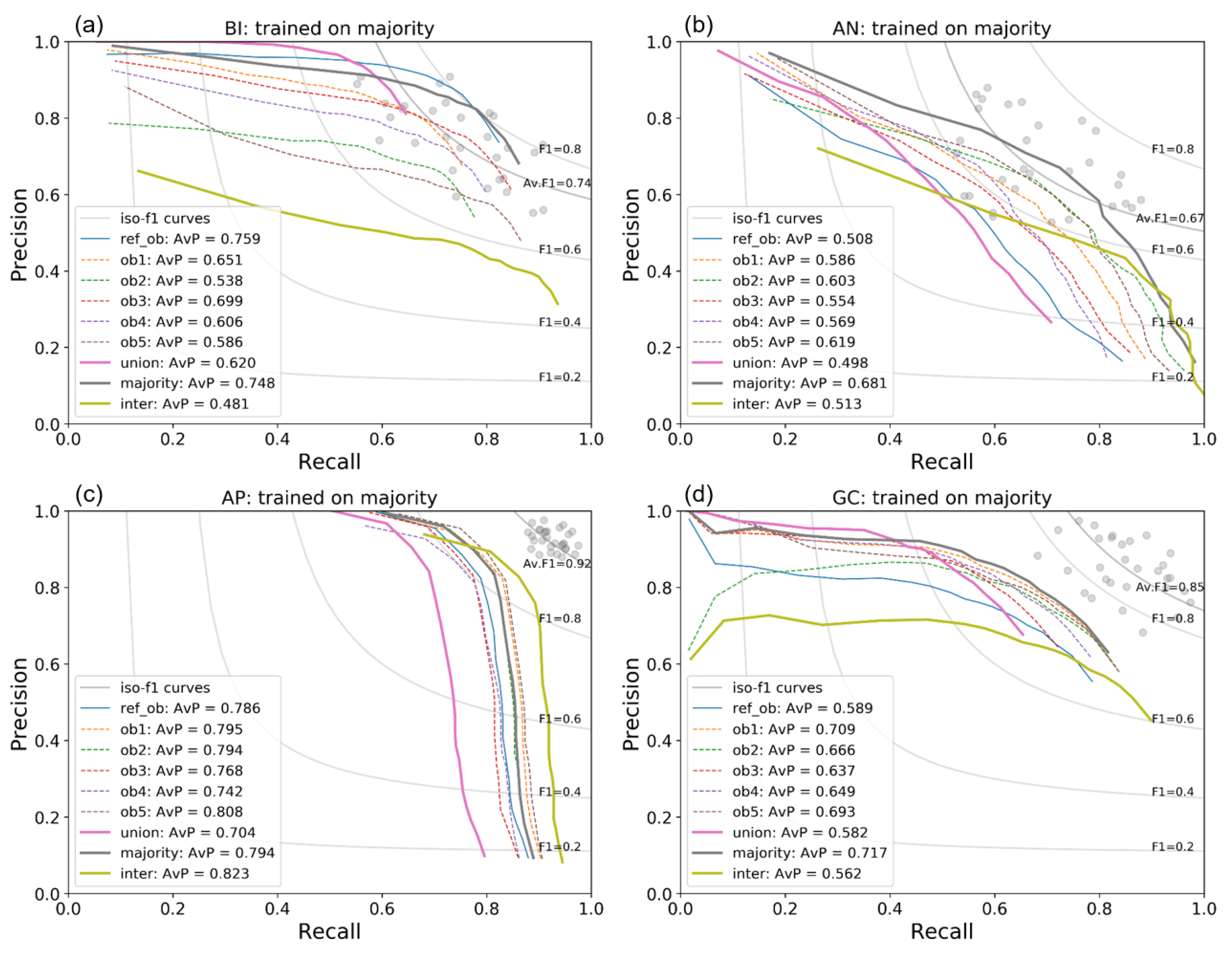
We present network results for each of our four islands, where each model was trained using our leave-one-island-out cross-validation (i.e., trained solely on image tiles from the three other islands). To assess the results of the network in the context of interobserver variation, we take the interobserver F1-scores from Table 2, and plot them as precision–recall points (Figure 4, grey points). We also add iso-F1 curves showing the average accuracy for reference (Figure 4, grey lines). For the network to reach human performance, the precision-recall curves should cut through the grey clusters.
3.2.1. Altering Assessment Ground Truth
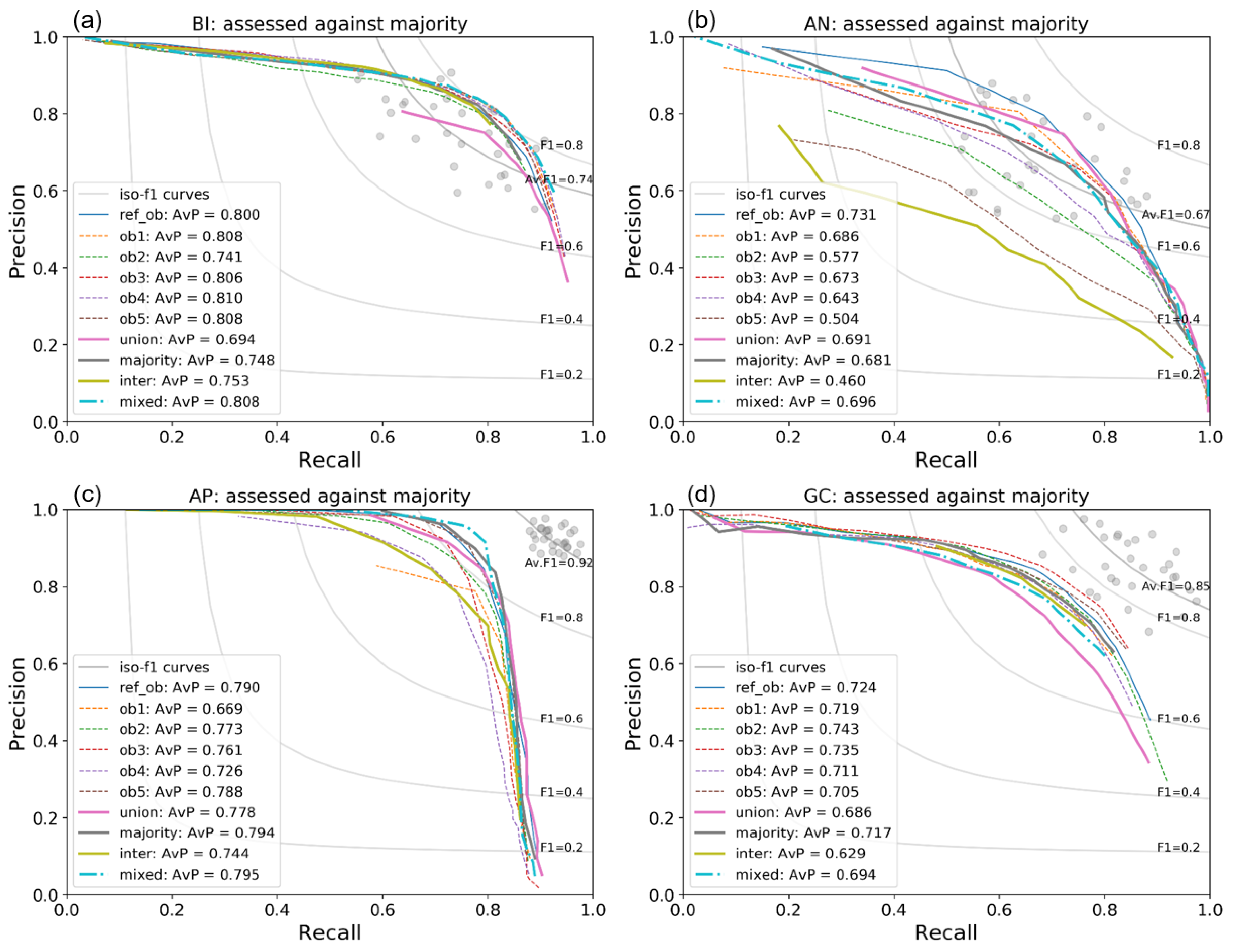
The results of assessing the output of the network against different ground truth labels are presented in Figure 4. We stress that all four models were trained with using the same ground truth (the majority vote), and all other model parameters were kept the same. We can see from the spread of precision-recall curves that our assessment of model performance can vary significantly depending on our chosen ground truth. At one extreme using the union gives us an overall lower recall, as many high uncertainty points (e.g., labelled by only one observer) are not predicted to be albatrosses by the network. On the other hand assessing against the intersection we get a high recall but lower precision, as more of the network predictions are assessed as false positives. We also see a range of results assessing against each individual observer, showing the pitfalls of using a single set of labels, as many studies currently do. For example, for AN using the reference observer labels would lead us to assess the model performing below human accuracy, whereas simply choosing another observer (e.g., observer 5) we would fall within the range (Figure 4b). The spread is more evident in the islands with lower observer agreement (BI and AN), opposed to those with higher observer agreement (AP and GC). On average, across all four islands, the best mean average precision score (mAP; Supplementary Table S3) comes from assessing against the majority vote (mAP = 0.73) and the worst using the intersection (mAP = 0.60). We also note that while models for BI and AN fall within the range of human performance (exceeding the average observer F1-scores of 0.74 and 0.67, respectively), for the other two images we do not hit this target.
3.2.2. Altering Training Ground Truth
We see that the network is relatively robust to using different ground truth labels at the training stage (Figure 5). For most of the islands there is little deviation in results when trained on either an individual observer, union, majority or intersection ground truth. The most notable exception to this is AN (Figure 5b), where we see a lot of variation, and a dramatic drop in recall-precision when training on the intersection labels (AvP = 0.460). This is likely to be because the network has only been trained using high confidence points from the three other islands, which means uncertain points (which Figure 3 showed account for over half the dataset in AN) are not predicted by the network at test stage. We also see that using different training labels can improve model performance when compared to training on the majority vote. For example in GC (Figure 5d) training with observer 3’s labels gives a better result (AvP = 0.735) compared to the majority (AvP = 0.717), and brings us nearer the level of interobserver accuracy. The mAP scores (Supplementary Table S3) show that on average the reference observer’s labels give us the best results across all images (mAP = 0.76). This is closely followed by the “mixed” ground truth (mAP = 0.75).
4. Discussion
4.1. Manual Counts
Analysis of manual counts show that the level of interobserver variation is significant, and depends on the properties of the individual images. For example, in our dataset we have very high interobserver agreement for AP (0.92), and much lower interobserver agreement for AN (0.67). Visual inspection of the images suggests the main reasons are the contrast between albatrosses and background vegetation, and the number of visually similar background features such as rocks. For demonstration we present examples of albatrosses which have been labelled by all six, exactly three, and only one observer in Figure 6. While points labelled by all six observes tend to have a clear contrast and relatively uniform background, for low confidence points there is often a very weak signature, or uneven background. For example many points labelled by one observer are in areas of rocky brown terrain. Even though the white dots themselves have a similar appearance to albatrosses, the context of the background may have lead other observers to discount them. For novice observers it may be beneficial to give further training, such as information on likely nesting habitat, or perform preprocessing steps to reduce the search area to only the most likely habitat regions. It may be possible to gain this information from metrics such as the normalised difference vegetation index [34], and from digital elevation models which could be used to exclude regions with steep slopes. These steps could also be incorporated into the automated approach, which would perhaps improve detection results and also reduce processing times.
Interestingly, AP observers have labelled points below cloud cover (Figure 6), in many cases with majority agreement. Viewed as isolated examples we would perhaps not expect to see such high confidence in these annotations, as the clouds mask out most colour information. This could be a consequence of the labelling procedure, where the image is scanned as a grid, allowing observers to build a wider picture of the distribution of albatrosses. If points below cloud cover are near a cluster of more clearly discernible albatrosses, then observers may be more likely to annotate them. To remove this bias, patches could be presented in a randomised way, to make interpretation of the images more standardised. It may also be interesting to investigate whether the cloud cover examples could be enhanced by using dehazing algorithms [35,36], to remove cloud cover as a preprocessing step. Incorporating the near-infrared (NIR) band could offer a means of achieving this, as research has shown NIR information can be combined with RGB channels to reduce the appearance of haze in images [37]. Enhancing RGB images by incorporating additional multispectral information could improve detection during manual analysis, and potentially reduce the amount of interobserver variation and uncertainty. Human observers could then benefit from the information provided in non-RGB bands (for WV-3 this includes NIR-1, NIR-2, red-edge, yellow and coastal), which can be trivially input to the CNN as imagery does not need to be visually interpretable. These approaches could benefit surveys of other species, for example it has been shown that the coastal band can aid detection of whales, since it penetrates further through the water column [4]. Methods for enhancing and adjusting images could also help to reduce variation in manual counts across different images.
4.2. Network Performance
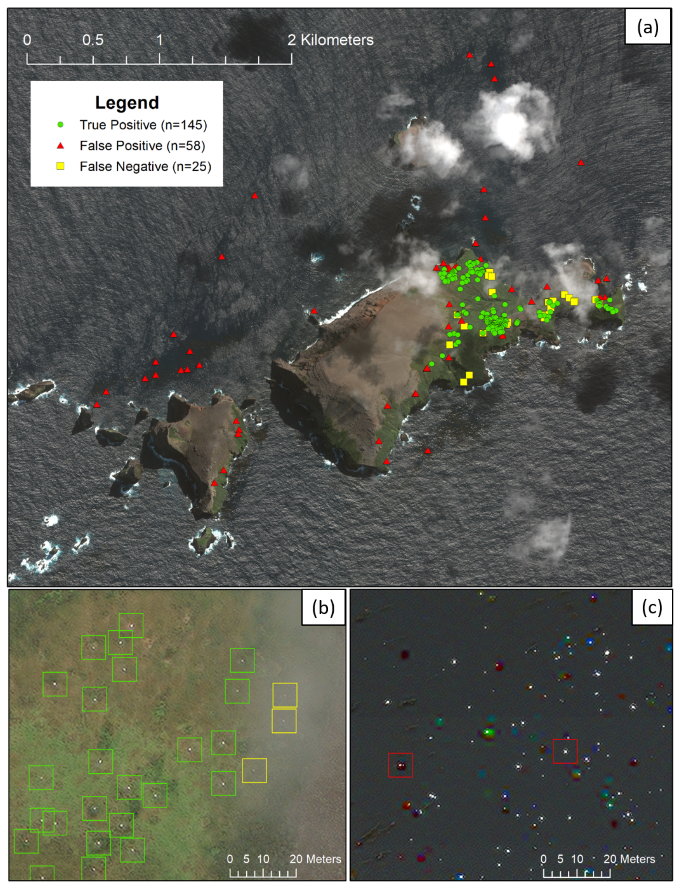
Our CNN results highlight the importance of assessing performance within the context of observer accuracy. This is particularly evident in AN, where our best performing networks achieve peak F1-scores of approximately 0.7. While in general we would aim to improve this score towards 100%, when we assess observer accuracy we find that these network results are already in the range of human performance (average F1-score of 0.67). This is also true for our results on BI, with an average observer accuracy of 0.74 and peak network performance of over 0.8. However even choosing the best scoring networks for AP and GC, we fall below our average observer F1-scores. In the case of AP, this can be attributed to two main reasons. The first is that, as discussed, many observers annotated points which fell below cloud cover. These contribute to the majority of false negatives when analysing our network predictions (in Figure 7 we present examples using the results of our majority vote trained CNN). As the network has not been presented with examples of cloud cover in the three training images, it is not surprising the network is unable to generalise in this case. The second is that spectral distortion over the ocean leads to a number of false positive results (Figure 7C). It is likely that the combination of bright white waves crests and strong spectral extremes lead to these false detections, as again these are patterns which are not present in the training data. In the case of GC we can see that many false positive results, which lower the precision score, are present in the same area away from the main colony site (Supplementary Figure S1d).
In order to improve detection results under cloud we could preprocess images using image dehazing, as discussed previously. This could improve clarity and aid both the manual and automated analysis of the imagery. An alternative would be to instead simulate cloud cover, and add it to a proportion of images at the training stage (for example, by adding perlin noise [38]). If the simulated cover is sufficiently accurate, this can be a means of artificially generating the examples needed to train the network. This being said, we recommend obtaining cloud free imagery wherever possible, as the certainty of our detections in thicker areas of cloud are limited both in manual and automated approaches. Similar augmentation approaches could be employed to deal with the false positives over the ocean in AP. Making the network more robust to this form of noise is important, as it could present itself differently in future imagery. Another alternative is to mask out areas of ocean before generating network predictions, which could be performed fairly quickly manually, or automatically using the normalised difference water index [34]. Masking out areas of ocean would have the dual benefit of decreasing the potential number of false positives, and reducing the processing time. This is also true for the false positive detections in GC, which fall outside the main colony area (Supplementary Figure S1). Again, input images could be manually preprocessed by experts to restrict the search to known colony locations. Even without these additions obvious false positives could be easily filtered out manually, with comparatively little effort. It is also important to note that results would almost certainly be improved by the addition of extra imagery, and the application of updated state-of-the-art CNN architectures which are rapidly evolving.
We find the choice of ground truth labels has an impact on both the training and assessment of our CNN. Choosing a single observer’s labels is not recommended, as we can see significant variation in results, particularly at the assessment stage. In terms of combining counts from multiple observers, using the majority vote can improve our assessment, as many low certainty points are removed from the ground truth. However this means discounting a large number of labels which, although low confidence, still contain useful information. At the training stage we found that using a mixture of labels can be a good alternative which avoids this problem. In the future other alternatives for combining ground truth could be investigated, including having a probabilistic ground truth (e.g., 1 if labelled by all observers, 0.5 if labelled by half, etc.). Observers could also be asked to assign a confidence class to each of their detections, for example if they think it is certain, likely, or possible. This method has been employed in surveys of larger species such as whales [39,40]. Giving observers the option to rank their detections in this way, rather than forcing a definite yes/no choice, may be equally informative as checking the agreement between multiple observers. This would potentially reduce the number of observers required to gauge uncertainty, although it may significantly increase the time taken to manually label images. Finally, there is potential to incorporate labels from different observers into the architecture of the CNN itself, as shown in recent research by Rodrigues et al. [41]. In this method a “crowd-layer” is added to the end of the network, allowing each observer to be modelled separately, only combining predictions in the final stages by the use of learned weights. They showed that modelling individual observers in this way can improve classification performance, and is a useful approach for any crowd-source annotated datasets.
5. Conclusions
While we have used Wandering Albatrosses as our study case, it is very likely that topics discussed in this paper apply to VHR satellite surveys of other species, as well as UAV and aerial surveys where image resolution is coarse and observer confidence is limited. For example, observer uncertainty has been noted in aerial studies where there is a low contrast between wildlife and background [42,43], and when flight height and camera resolution results in comparitively low ground sample resolution in relation to the size of the target animal [44]. In particular we show that (1) manual counts of wildlife in satellite imagery can vary significantly between observers, and importantly observer confidence may differ between images, (2) new images may present challenges to CNNs trained on small VHR satellite datasets and (3) the choice of ground truth can impact supervised schemes at both the assessment and training stage. We also highlight the importance of assessing results of automated approaches within the context of interobserver variation, for each unique image, to accurately gauge performance.
In general, the results of our automated CNN approach are promising; in our leave-one-island-out cross-validation we match human performance for two out of four islands, and for the other two misclassifications are mostly obvious and therefore easy to filter. We hope that these methods can facilitate future satellite surveys of Wandering Albatrosses, with increased frequency and reduced cost. In particular, as the global breeding population of Wandering Albatrosses nest in relatively few locations (approximately 18% on South Georgia, 44% on Prince Edward Islands and 38% on Crozet and Kerguelen Islands [29]), the potential to conduct a global population survey using VHR satellite is feasible. The methods could also be adapted for other species, such as the Northern Royal Albatross, which were shown to be visible in previous studies [14]. If repeated at regular intervals this would vastly improve our knowledge of spatial and temporal population dynamics, for a species which is of high conservation concern.
Supplementary Materials
The following are available online at https://www.mdpi.com/2072-4292/12/12/2026/s1, Table S1: Satellite image details, Table S2: Albatross examples, Table S3: Network mAP scores, Figure S1: Detection maps for all islands.
Author Contributions
Conceptualization, E.B., M.M and P.T.F.; methodology, E.B., G.F. and M.M.; data curation, P.T.F. and E.B.; software E.B. and G.F.; writing—original draft preparation, E.B.; writing—review and editing, E.B., P.T.F., G.F. and M.M. All authors provided comments. All authors have read and agreed to the published version of the manuscript.
Funding
This research was funded by the Natural Environmental Research Council through the NEXUSS CDT, grant number NE/N012070/1, titled “Automated UAV and Satellite Image Analysis for Wildlife Monitoring”.
Acknowledgments
The WV-3 imagery used in this research was courtesy of DigitalGlobe, a Maxar company. The authors thank Henri Weimerskirch for allowing the use of the AP and GC images, which were acquired as part of a separate study, and additionally thank all volunteers who kindly gave up their time to annotate the dataset. We gratefully acknowledge the support of NVIDIA Corporation with the donation of the Titan Xp GPU used for this research.
Conflicts of Interest
The authors declare no conflicts of interest.
Abbreviations
The following abbreviations are used in this manuscript:
| VHR | Very high resolution |
| WV-3 | WorldView-3 |
| CNN | Convolutional neural network |
| AvP | Average precision |
| mAP | Mean average precision |
References
- Pettorelli, N.; Laurance, W.F.; O’Brien, T.G.; Wegmann, M.; Nagendra, H.; Turner, W. Satellite remote sensing for applied ecologists: Opportunities and challenges. J. Appl. Ecol. 2014, 51, 839–848. [Google Scholar] [CrossRef]
- Hollings, T.; Burgman, M.; van Andel, M.; Gilbert, M.; Robinson, T.; Robinson, A. How do you find the green sheep? A critical review of the use of remotely sensed imagery to detect and count animals. Methods Ecol. Evol. 2018. [Google Scholar] [CrossRef]
- Witmer, G.W. Wildlife population monitoring: Some practical considerations. Wildl. Res. 2005, 32, 259–263. [Google Scholar] [CrossRef]
- Fretwell, P.T.; Staniland, I.J.; Forcada, J. Whales from space: Counting southern right whales by satellite. PLoS ONE 2014, 9, e88655. [Google Scholar] [CrossRef] [Green Version]
- Oishi, Y.; Matsunaga, T. Support system for surveying moving wild animals in the snow using aerial remote-sensing images. Int. J. Remote Sens. 2014, 35, 1374–1394. [Google Scholar] [CrossRef]
- Anderson, K.; Gaston, K.J. Lightweight unmanned aerial vehicles will revolutionize spatial ecology. Front. Ecol. Environ. 2013, 11, 138–146. [Google Scholar] [CrossRef] [Green Version]
- Rowcliffe, J.M.; Carbone, C. Surveys using camera traps: Are we looking to a brighter future? Anim. Conserv. 2008, 11, 185–186. [Google Scholar] [CrossRef]
- LaRue, M.A.; Stapleton, S.; Anderson, M. Feasibility of using high-resolution satellite imagery to assess vertebrate wildlife populations. Conserv. Biol. 2017, 31, 213–220. [Google Scholar] [CrossRef]
- Xue, Y.; Wang, T.; Skidmore, A.K. Automatic counting of large mammals from very high resolution panchromatic satellite imagery. Remote Sens. 2017, 9, 878. [Google Scholar] [CrossRef] [Green Version]
- LaRue, M.A.; Stapleton, S. Estimating the abundance of polar bears on Wrangel Island during late summer using high-resolution satellite imagery: A pilot study. Polar Biol. 2018, 41, 2621–2626. [Google Scholar] [CrossRef]
- Borowicz, A.; Le, H.; Humphries, G.; Nehls, G.; Höschle, C.; Kosarev, V.; Lynch, H.J. Aerial-trained deep learning networks for surveying cetaceans from satellite imagery. PLoS ONE 2019, 14, e0212532. [Google Scholar] [CrossRef] [PubMed]
- Wang, D.; Shao, Q.; Yue, H. Surveying Wild Animals from Satellites, Manned Aircraft and Unmanned Aerial Systems (UASs): A Review. Remote Sens. 2019, 11, 1308. [Google Scholar] [CrossRef] [Green Version]
- Larue, M.A.; Stapleton, S.; Porter, C.; Atkinson, S.; Atwood, T.; Dyck, M.; Lecomte, N. Testing methods for using high-resolution satellite imagery to monitor polar bear abundance and distribution. Wildl. Soc. Bull. 2015, 39, 772–779. [Google Scholar] [CrossRef]
- Fretwell, P.T.; Scofield, P.; Phillips, R.A. Using super-high resolution satellite imagery to census threatened albatrosses. Ibis 2017, 159, 481–490. [Google Scholar] [CrossRef]
- Weinstein, B.G. A computer vision for animal ecology. J. Animal Ecol. 2017. [Google Scholar] [CrossRef]
- LeCun, Y.A.; Bengio, Y.; Hinton, G.E. Deep learning. Nature 2015, 521, 436–444. [Google Scholar] [CrossRef]
- Deng, J.; Dong, W.; Socher, R.; Li, L.J.; Li, K.; Fei-Fei, L. ImageNet: A Large-Scale Hierarchical Image Database. In Proceedings of the 2009 IEEE Conference on Computer Vision and Pattern Recognition, Miami, FL, USA, 20–25 June 2009. [Google Scholar]
- Krizhevsky, A.; Sutskever, I.; Hinton, G.E. Imagenet classification with deep convolutional neural networks. Adv. Neural Inf. Process. Syst. 2012, 1097–1105. [Google Scholar] [CrossRef]
- Gray, P.C.; Fleishman, A.B.; Klein, D.J.; McKown, M.W.; Bézy, V.S.; Lohmann, K.J.; Johnston, D.W. A convolutional neural network for detecting sea turtles in drone imagery. Methods Ecol. Evol. 2019, 10, 345–355. [Google Scholar] [CrossRef]
- Norouzzadeh, M.S.; Nguyen, A.; Kosmala, M.; Swanson, A.; Palmer, M.S.; Packer, C.; Clune, J. Automatically identifying, counting, and describing wild animals in camera-trap images with deep learning. Proc. Natl. Acad. Sci. USA 2018, 115, E5716–E5725. [Google Scholar] [CrossRef] [Green Version]
- Hänsch, R.; Hellwich, O. The Truth About Ground Truth: Label Noise in Human-Generated Reference Data. In Proceedings of the IGARSS 2019—2019 IEEE International Geoscience and Remote Sensing Symposium, Yokohama, Japan, 28 July–2 August 2019; pp. 5594–5597. [Google Scholar]
- Weimerskirch, H.; Delord, K.; Barbraud, C.; Le Bouard, F.; Ryan, P.G.; Fretwell, P.; Marteau, C. Status and trends of albatrosses in the French Southern Territories, Western Indian Ocean. Polar Biol. 2018, 41, 1963–1972. [Google Scholar] [CrossRef]
- Phillips, R.; Gales, R.; Baker, G.; Double, M.; Favero, M.; Quintana, F.; Tasker, M.; Weimerskirch, H.; Uhart, M.; Wolfaardt, A. The conservation status and priorities for albatrosses and large petrels. Biol. Conserv. 2016, 201, 169–183. [Google Scholar] [CrossRef]
- Fretwell, P.T.; LaRue, M.A.; Morin, P.; Kooyman, G.L.; Wienecke, B.; Ratcliffe, N.; Fox, A.J.; Fleming, A.H.; Porter, C.; Trathan, P.N. An emperor penguin population estimate: The first global, synoptic survey of a species from space. PLoS ONE 2012, 7, e33751. [Google Scholar] [CrossRef]
- LaRue, M.A.; Lynch, H.; Lyver, P.; Barton, K.; Ainley, D.; Pollard, A.; Fraser, W.; Ballard, G. A method for estimating colony sizes of Adélie penguins using remote sensing imagery. Polar Biol. 2014, 37, 507–517. [Google Scholar] [CrossRef]
- Naveen, R.; Lynch, H.J.; Forrest, S.; Mueller, T.; Polito, M. First direct, site-wide penguin survey at Deception Island, Antarctica, suggests significant declines in breeding chinstrap penguins. Polar Biol. 2012, 35, 1879–1888. [Google Scholar] [CrossRef]
- Hughes, B.J.; Martin, G.R.; Reynolds, S.J. The use of Google EarthTM satellite imagery to detect the nests of masked boobies Sula dactylatra. Wildl. Biol. 2011, 17, 210–216. [Google Scholar] [CrossRef] [Green Version]
- Bowler, E.; Fretwell, P.T.; French, G.; Mackiewicz, M. Using Deep Learning to Count Albatrosses from Space. In Proceedings of the IGARSS 2019—2019 IEEE International Geoscience and Remote Sensing Symposium, Yokohama, Japan, 28 July–2 August 2019; pp. 10099–10102. [Google Scholar]
- BirdLife International. Species Factsheet: Diomedea Exulans. 2020. Available online: http://www.birdlife.org (accessed on 8 June 2020).
- Ronneberger, O.; Fischer, P.; Brox, T. U-Net: Convolutional Networks for Biomedical Image Segmentation. Miccai 2015, 234–241. [Google Scholar] [CrossRef] [Green Version]
- Simonyan, K.; Zisserman, A. Very Deep Convolutional Networks for Large-Scale Image Recognition. In Proceedings of the International Conference on Learning Representations, San Diego, CA, USA, 7–9 May 2015. [Google Scholar]
- Forsyth, D.A.; Ponce, J. Computer Vision: A Modern Approach; Prentice Hall Professional Technical Reference: Upper Saddle River, NJ, USA, 2002. [Google Scholar]
- Lin, T.Y.; Goyal, P.; Girshick, R.; He, K.; Dollár, P. Focal loss for dense object detection. In Proceedings of the IEEE International Conference on Computer Vision, Venice, Italy, 22–29 October 2017; pp. 2980–2988. [Google Scholar]
- Liang, S.; Wang, J. Advanced Remote Sensing: Terrestrial Information Extraction and Applications; Academic Press: Cambridge, MA, USA, 2019. [Google Scholar]
- Guo, F.; Cai, Z.x.; Xie, B.; Tang, J. Review and prospect of image dehazing techniques. Jisuanji Yingyong/J. Comput. Appl. 2010, 30, 2417–2421. [Google Scholar] [CrossRef]
- Jiang, H.; Lu, N. Multi-scale residual convolutional neural network for haze removal of remote sensing images. Remote Sens. 2018, 10, 945. [Google Scholar] [CrossRef] [Green Version]
- Fredembach, C.; Süsstrunk, S. Colouring the near-infrared. Soc. Imag. Sci. Technol. 2008, 2008, 176–182. [Google Scholar]
- Lee, K.Y.; Sim, J.Y. Cloud Removal of Satellite Images Using Convolutional Neural Network With Reliable Cloudy Image Synthesis Model. In Proceedings of the 2019 IEEE International Conference on Image Processing (ICIP), Taipei, Taiwan, 22–25 September 2019; pp. 3581–3585. [Google Scholar]
- Fretwell, P.T.; Jackson, J.A.; Encina, M.J.U.; Häussermann, V.; Alvarez, M.J.P.; Olavarría, C.; Gutstein, C.S. Using remote sensing to detect whale strandings in remote areas: The case of sei whales mass mortality in Chilean Patagonia. PLoS ONE 2019, 14, e0222498. [Google Scholar]
- Cubaynes, H.C.; Fretwell, P.T.; Bamford, C.; Gerrish, L.; Jackson, J.A. Whales from space: Four mysticete species described using new VHR satellite imagery. Mar. Mamm. Sci. 2019, 35, 466–491. [Google Scholar] [CrossRef]
- Rodrigues, F.; Pereira, F.C. Deep learning from crowds. In Proceedings of the Thirty-Second AAAI Conference on Artificial Intelligence, New Orleans, LA, USA, 2–7 February 2018. [Google Scholar]
- Chabot, D.; Bird, D.M. Evaluation of an off-the-shelf unmanned aircraft system for surveying flocks of geese. Waterbirds 2012, 35, 170–174. [Google Scholar] [CrossRef]
- Patterson, C.; Koski, W.; Pace, P.; McLuckie, B.; Bird, D.M. Evaluation of an unmanned aircraft system for detecting surrogate caribou targets in Labrador. J. Unmanned Veh. Syst. 2015, 4, 53–69. [Google Scholar] [CrossRef] [Green Version]
- Brack, I.V.; Kindel, A.; Oliveira, L.F.B. Detection errors in wildlife abundance estimates from Unmanned Aerial Systems (UAS) surveys: Synthesis, solutions, and challenges. Methods Ecol. Evol. 2018, 9, 1864–1873. [Google Scholar] [CrossRef]
Figure 1.
Examples of albatrosses in the four islands, as viewed in ArcMap 10.5. (a) Bird Island. (b) Annenkov Island. (c) Apotres Island. (d) Grande Coulee. Imagery from DigitalGlobe Products. WorldView3© 2020 DigitalGlobe, Inc., a Maxar company.
Figure 1.
Examples of albatrosses in the four islands, as viewed in ArcMap 10.5. (a) Bird Island. (b) Annenkov Island. (c) Apotres Island. (d) Grande Coulee. Imagery from DigitalGlobe Products. WorldView3© 2020 DigitalGlobe, Inc., a Maxar company.

Figure 2.
Diagram of the U-Net architecture and training procedure. The input channels are stacked and fed forward through the network. The contracting path applies repeated convolution and max pooling operations to extract feature maps, while in the expanding path these are upsampled and stacked with features cropped from the corresponding layer in the contracting path. The output is a heatmap, which is compared against the ground truth using focal loss. This loss is used to train the network, through backpropagation of errors and Adam optimization.

Figure 3.
The distribution of points labelled by multiple observers.

Figure 4.
Precision–recall curves assessed against different sets of ground truth for (a) Bird Island, (b) Annenkov Island, (c) Apotres Island and (d) Grande Coulee. We train the models using leave-one- island-out cross-validation, and the majority vote labels as training ground truth. Gray points show the individual interobserver precision–recall points, and grey lines show the corresponding F1-scores. Coloured lines show the precision–recall curves when assessing model output against different ground truth labels. The average precision (AvP) is the area under the precision–recall curve.

Figure 5.
Precision–recall curves for models trained on different ground truth labels, for (a) Bird Island, (b) Annenkov Island, (c) Apotres Island and (d) Grande Coulee. We train each model using leave-one-island-out cross validation, and a different set of ground truth labels (coloured lines). All results are assessed against the majority vote labels. Grey points show the individual interobserver precision–recall points, and grey lines show the corresponding F1-scores. The average precision (AvP) is the area under the precision–recall curve.

Figure 6.
Examples of albatrosses labelled by all six, exactly three, and only one observer, for each of the four islands. Imagery from DigitalGlobe Products. WorldView3© 2020 DigitalGlobe, Inc., a Maxar company.
Figure 6.
Examples of albatrosses labelled by all six, exactly three, and only one observer, for each of the four islands. Imagery from DigitalGlobe Products. WorldView3© 2020 DigitalGlobe, Inc., a Maxar company.

Figure 7.
Detection results for AP. We use the CNN trained and assessed using the majority vote, and threshold predictions at 0.55. (a) The results over the whole image. (b) An example of false negatives under cloud cover. (c) An example of false positives in the ocean, cause by spectral noise and wave crests. Imagery from DigitalGlobe Products. WorldView3© 2020 DigitalGlobe, Inc., a Maxar company.


Table 1.
Total counts with the mean, standard deviation and percent deviation for each island.
| ref_ob | ob1 | ob2 | ob3 | ob4 | ob5 | Mean ± std | % dev | |
|---|---|---|---|---|---|---|---|---|
| Bird Island | 985 | 994 | 763 | 792 | 846 | 612 | 832 ± 145 | 17 |
| Annenkov | 161 | 155 | 116 | 177 | 174 | 120 | 151 ± 26 | 18 |
| Apotres | 171 | 165 | 168 | 177 | 174 | 162 | 170 ± 6 | 3 |
| Grande Coulee | 649 | 690 | 656 | 840 | 741 | 638 | 702 ± 77 | 11 |
Table 2.
Accuracy (as F1-score) between observer labels for (a) Bird Island, (b) Annenkov Island, (c) Apotres Island and (d) Grande Coulee. We highlight the worst (red) and best (green) scores, and calculate the mean F1-score per observer, as well as the average F1 score (Av. F1) for each island. Averages exclude the 100% F1-scores achieved when comparing an observer against themselves.
| (a) | BI: Av. F1 = 0.74 | (b) | AN: Av. F1 = 0.67 | |||||||||||
|---|---|---|---|---|---|---|---|---|---|---|---|---|---|---|
| ref_ob | ob1 | ob2 | ob3 | ob4 | ob5 | ref_ob | ob1 | ob2 | ob3 | ob4 | ob5 | |||
| ref_ob | 1.00 | 0.81 | 0.72 | 0.81 | 0.78 | 0.68 | ref_ob | 1.00 | 0.63 | 0.62 | 0.57 | 0.57 | 0.60 | |
| ob1 | 0.81 | 1.00 | 0.70 | 0.79 | 0.75 | 0.69 | ob1 | 0.63 | 1.00 | 0.72 | 0.73 | 0.70 | 0.73 | |
| ob2 | 0.72 | 0.70 | 1.00 | 0.74 | 0.70 | 0.66 | ob2 | 0.62 | 0.72 | 1.00 | 0.68 | 0.70 | 0.78 | |
| ob3 | 0.81 | 0.79 | 0.74 | 1.00 | 0.78 | 0.73 | ob3 | 0.57 | 0.73 | 0.68 | 1.00 | 0.66 | 0.69 | |
| ob4 | 0.78 | 0.75 | 0.70 | 0.78 | 1.00 | 0.70 | ob4 | 0.57 | 0.70 | 0.70 | 0.66 | 1.00 | 0.67 | |
| ob5 | 0.68 | 0.69 | 0.66 | 0.73 | 0.70 | 1.00 | ob5 | 0.60 | 0.73 | 0.78 | 0.69 | 0.67 | 1.00 | |
| mean | 0.76 | 0.75 | 0.70 | 0.77 | 0.74 | 0.69 | mean | 0.60 | 0.70 | 0.70 | 0.67 | 0.66 | 0.70 | |
| (c) | AP: Av. F1 = 0.92 | (d) | GC: Av. F1 = 0.85 | |||||||||||
| ref_ob | ob1 | ob2 | ob3 | ob4 | ob5 | ref_ob | ob1 | ob2 | ob3 | ob4 | ob5 | |||
| ref_ob | 1.00 | 0.93 | 0.91 | 0.93 | 0.89 | 0.92 | ref_ob | 1.00 | 0.83 | 0.82 | 0.77 | 0.79 | 0.78 | |
| ob1 | 0.93 | 1.00 | 0.95 | 0.94 | 0.93 | 0.95 | ob1 | 0.83 | 1.00 | 0.91 | 0.87 | 0.89 | 0.88 | |
| ob2 | 0.91 | 0.95 | 1.00 | 0.91 | 0.91 | 0.93 | ob2 | 0.82 | 0.91 | 1.00 | 0.85 | 0.87 | 0.86 | |
| ob3 | 0.93 | 0.94 | 0.91 | 1.00 | 0.92 | 0.93 | ob3 | 0.77 | 0.87 | 0.85 | 1.00 | 0.88 | 0.82 | |
| ob4 | 0.89 | 0.93 | 0.91 | 0.92 | 1.00 | 0.91 | ob4 | 0.79 | 0.89 | 0.87 | 0.88 | 1.00 | 0.86 | |
| ob5 | 0.92 | 0.95 | 0.93 | 0.93 | 0.91 | 1.00 | ob5 | 0.78 | 0.88 | 0.86 | 0.82 | 0.86 | 1.00 | |
| mean | 0.92 | 0.94 | 0.92 | 0.93 | 0.91 | 0.93 | mean | 0.80 | 0.87 | 0.86 | 0.84 | 0.86 | 0.84 | |
Table 3.
Accuracy (as F1-score) when assessing each observer’s predictions (rows) against all options for combined ground truths (ranging from taking the union of all observer annotations, through to the intersection. Results for (a) Bird Island, (b) Annenkov Island, (c) Apotres Island and (d) Grande Coulee.
| (a) | BI | (b) | AN | |||||||||||
|---|---|---|---|---|---|---|---|---|---|---|---|---|---|---|
| union | ≥ 2 | ≥ 3 | ≥ 4 | ≥ 5 | inter | union | ≥ 2 | ≥ 3 | ≥ 4 | ≥ 5 | inter | |||
| ref_ob | 0.83 | 0.91 | 0.88 | 0.83 | 0.75 | 0.55 | ref_ob | 0.67 | 0.66 | 0.70 | 0.69 | 0.70 | 0.56 | |
| ob1 | 0.83 | 0.87 | 0.87 | 0.82 | 0.75 | 0.54 | ob1 | 0.66 | 0.85 | 0.84 | 0.81 | 0.78 | 0.57 | |
| ob2 | 0.71 | 0.77 | 0.79 | 0.80 | 0.78 | 0.65 | ob2 | 0.54 | 0.78 | 0.85 | 0.88 | 0.84 | 0.70 | |
| ob3 | 0.72 | 0.85 | 0.89 | 0.89 | 0.83 | 0.64 | ob3 | 0.72 | 0.82 | 0.79 | 0.74 | 0.70 | 0.52 | |
| ob4 | 0.75 | 0.84 | 0.85 | 0.84 | 0.79 | 0.61 | ob4 | 0.71 | 0.81 | 0.77 | 0.74 | 0.71 | 0.53 | |
| ob5 | 0.61 | 0.73 | 0.78 | 0.80 | 0.82 | 0.75 | ob5 | 0.55 | 0.76 | 0.84 | 0.88 | 0.85 | 0.68 | |
| mean | 0.74 | 0.83 | 0.84 | 0.83 | 0.78 | 0.62 | mean | 0.64 | 0.78 | 0.80 | 0.79 | 0.76 | 0.59 | |
| (c) | AP | (d) | GC | |||||||||||
| union | ≥2 | ≥3 | ≥4 | ≥5 | inter | union | ≥2 | ≥3 | ≥4 | ≥5 | inter | |||
| ref_ob | 0.91 | 0.94 | 0.94 | 0.93 | 0.94 | 0.90 | ref_ob | 0.79 | 0.83 | 0.85 | 0.85 | 0.85 | 0.83 | |
| ob1 | 0.89 | 0.96 | 0.98 | 0.98 | 0.97 | 0.92 | ob1 | 0.82 | 0.92 | 0.95 | 0.95 | 0.92 | 0.80 | |
| ob2 | 0.90 | 0.95 | 0.94 | 0.96 | 0.95 | 0.91 | ob2 | 0.80 | 0.91 | 0.94 | 0.95 | 0.92 | 0.82 | |
| ob3 | 0.92 | 0.96 | 0.96 | 0.95 | 0.94 | 0.88 | ob3 | 0.92 | 0.92 | 0.90 | 0.88 | 0.83 | 0.71 | |
| ob4 | 0.92 | 0.95 | 0.94 | 0.93 | 0.92 | 0.89 | ob4 | 0.85 | 0.93 | 0.93 | 0.91 | 0.88 | 0.76 | |
| ob5 | 0.88 | 0.93 | 0.95 | 0.96 | 0.97 | 0.93 | ob5 | 0.78 | 0.87 | 0.90 | 0.90 | 0.91 | 0.84 | |
| mean | 0.91 | 0.95 | 0.95 | 0.95 | 0.95 | 0.90 | mean | 0.83 | 0.90 | 0.91 | 0.91 | 0.89 | 0.79 | |
© 2020 by the authors. Licensee MDPI, Basel, Switzerland. This article is an open access article distributed under the terms and conditions of the Creative Commons Attribution (CC BY) license (http://creativecommons.org/licenses/by/4.0/).
Share and Cite
MDPI and ACS Style
Bowler, E.; Fretwell, P.T.; French, G.; Mackiewicz, M. Using Deep Learning to Count Albatrosses from Space: Assessing Results in Light of Ground Truth Uncertainty. Remote Sens. 2020, 12, 2026. https://doi.org/10.3390/rs12122026
AMA Style
Bowler E, Fretwell PT, French G, Mackiewicz M. Using Deep Learning to Count Albatrosses from Space: Assessing Results in Light of Ground Truth Uncertainty. Remote Sensing. 2020; 12(12):2026. https://doi.org/10.3390/rs12122026
Chicago/Turabian StyleBowler, Ellen, Peter T. Fretwell, Geoffrey French, and Michal Mackiewicz. 2020. "Using Deep Learning to Count Albatrosses from Space: Assessing Results in Light of Ground Truth Uncertainty" Remote Sensing 12, no. 12: 2026. https://doi.org/10.3390/rs12122026
Note that from the first issue of 2016, this journal uses article numbers instead of page numbers. See further details here.