Game Control Methods Comparison when Avoiding Collisions with Multiple Objects Using Radar Remote Sensing


Faculty of Marine Electrical Engineering, Gdynia Maritime University, 81-225 Gdynia, Poland
Remote Sens. 2020, 12(10), 1573; https://doi.org/10.3390/rs12101573
Submission received: 11 April 2020
/
Revised: 12 May 2020
/
Accepted: 13 May 2020
/
Published: 15 May 2020
(This article belongs to the Section AI Remote Sensing)
Abstract
:This article formulates the concept of games in the field of process control theory in marine sciences and reviews the literature on the possible applications of games. The possible types of game control processes for moving objects are presented. A computer-aided object safe control in the game environment, with an appropriate steering system, is described based on radar remote sensing in order to avoid collisions with many other objects that are encountered. First, the basic model of object movement in the game environment is presented as a differential game with many objects, described by appropriate game state equations, state and steering restrictions, and a quality control index in the form of an integral and final payment of the game. Next, the surrogate models of the differential game are described in detail for the development of practical computer control programs using positional and matrix game models. Particular attention, in each type of game, is paid to the aspect of cooperation or lack of cooperation between objects in making maneuvering decisions. A computer simulation illustrates these considerations with game control programs at a sea-crossing situation where multiple objects were encountered. Safe object trajectories are compared using two methods of game control using positional and matrix game models while also considering cases with cooperation or non-cooperation of objects.
1. Introduction
One of the most important problems that occurs in maritime transport is the prevention of collisions with objects, as described by Bist and Cahill [1,2]. To this end, it is mandatory that all objects are equipped with the remote sensing Automatic Radar Plotting Aid (ARPA) system, which tracks the movement of the objects that are encountered, calculates the parameters of their approach and allows for a trial maneuver for the most dangerous object to take into account the rules from the International Regulations for Preventing Collisions at Sea (COLREGs). Then, whether such a course or speed change maneuver is safe for other objects is assessed. If it is not secure, then the selection and trial maneuver are repeated for a new dangerous object. This solution to the anti-collision problem only works in situations where several objects pass each other. When a larger number of objects pass, it is necessary to use computer-aided maneuvering decisions in order to calculate all the possible solutions of the task and to propose one of the best ones, i.e., the optimal solution. At the same time, the optimization is as good as the mathematical model of the object control process is adequate. There are deterministic models described in References [3,4,5,6,7,8,9,10,11,12,13,14]; Blaich et al. [15] introduced a probabilistic model and Lazarowska and Tomera [16,17] presented a heuristic, notably, the swarm of particles model, as well as models using artificial intelligence, which were used in References [18,19,20,21,22,23,24,25,26] and game theory formulated, which was used in References [27,28,29,30,31].
The purpose of this review is to refer the considerations to the last method mentioned above through a detailed comparative analysis of the methods of game object control in collision situations with many objects passing by using radar remote sensing. The main premise for these considerations is that the navigator’s subjectivity in assessing the navigational situation, taking into account the rules of the sea law COLREGs, as well as the possibility of making a mistake and contributing to a collision situation as a conflict situation, has a great impact here. Game theory, which is a chapter of modern mathematics, including the theory of accidental events and the construction and analysis of their models, comes to the rescue. The conflict may be military, political, social, or economic, where there is a game with nature and there is the application of object steering, that is, when they interact, the impact disturbances or other objects can be seen. Therefore, it is appropriate to treat the process of passing objects safely as a game control, taking into account the cooperation or lack of cooperation between objects. The problem of collision-free sea control strategies has already appeared in Isaacs [32], the creator of differential game theory, and has been developed by many authors, especially object control in conditions of uncertainty. According to the authors [33,34,35], determining anti-collision strategies is easy, except for the uncertainty of the data, the results from harsh weather, high sea levels, as well as the actions of other objects and the navigator’s subjectivity in maneuvering decisions and imprecise character recommendations of international collision regulations COLREGs. Dockner et al. and Baba et al. [36,37] stated that the topic of defining safe strategies is still valid, due to the constantly increasing vessel traffic in individual water bodies; on the one hand, increasing the requirements of safe navigation and the safety of the environment; on the other, increasing the operational capacity of computer-assisted navigators. According to Breton et al. and Sanchez-Soriano [38,39], the largest type of game relates to the motion control of objects, including autonomous and non-autonomous marine objects, which are differential games.
This review concerns the comparative analysis of the applications of certain types of games, leading to the synthesis of algorithms of computer-aided navigator decisions in the safe maneuvering of an object in difficult and complex collision situations at sea.
2. Game Control Process of Multiple Objects Movement
2.1. General Description
On the basis Haurie et al. and Mesterton-Gibbons [40,41,42], the movement of objects in time describes the system of state equations:
where xi(t) is the function that describes the state of the control process; uj(t) is the function that describes how the j-th object controls in the form of its i-th strategies; t is the time; N is the permissible object strategies number; J is the object’s number.
According Osborne and Broek et al. [43,44], for the class often considered in the control technique of non-coalition games, the most beneficial conduct of the player is to minimize the goal function in the form of a functional:
where foj is the integral payoff and f is the final payoff.
The strategy of the j-th object leads to a game balance situation that is determined by Nash [45] equilibrium points. The optimal control of the j-th player, as an object or transport process, is determined from the following relationship:
Based on [46,47,48], it can be assumed that the task of developing the game control system is solved in two stages, corresponding to sufficient and necessary conditions to resolve the game J participants. Generally, there are two types of game controls: programming uj(t) and positioning uj[x(t)]. The main game control systems are positioning systems to control the position of objects, and also the feedback systems that represent the positional game.
2.2. Types of Object Traffic Game Control
The movement of objects takes place under the influence of controls on their movement, from U sets of possible strategies:
—possible strategies set of own object (OO);
—possible strategies set of j-th object.
- —leads to the shortest distance between subjects, often during the dangerous objects approach or when transferring cargo at sea.
- —this means an anti-collision maneuver to achieve the value of the smallest distance to j-th object, which is greater than the apparent safety distance Ds that is determined under the given conditions:where Dj min is the distance of the closest point of approach; Dj is the distance to the encountered j-th object; Ds is the safe distance of approach.
- —this means stabilizing the course or trajectory.
The following types of object traffic controls can be distinguished:
Case 1: Two-sided conflict game situations ,
Case 2: One-sided conflict game situations .
This happens in cases of incorrect assessment of the proximity situation by one object, while the other object does not observe the situation. It can also take place when one of the objects has a malfunctioning ARPA system or when the weather conditions are very bad, leading to the disappearance of the object’s echoes.
Case 3: Avoiding collisions by the following:
- Maneuvers of own object , for example, by changing a course Δψ and/or speed ΔV,
- Maneuvers of the j-th object ,
- Cooperating maneuvers .
Case 4: Objects meeting .
Case 5: Stabilization of the course or trajectory .
2.3. Computer-Aided Object Safe Control in the Game Environment
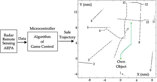
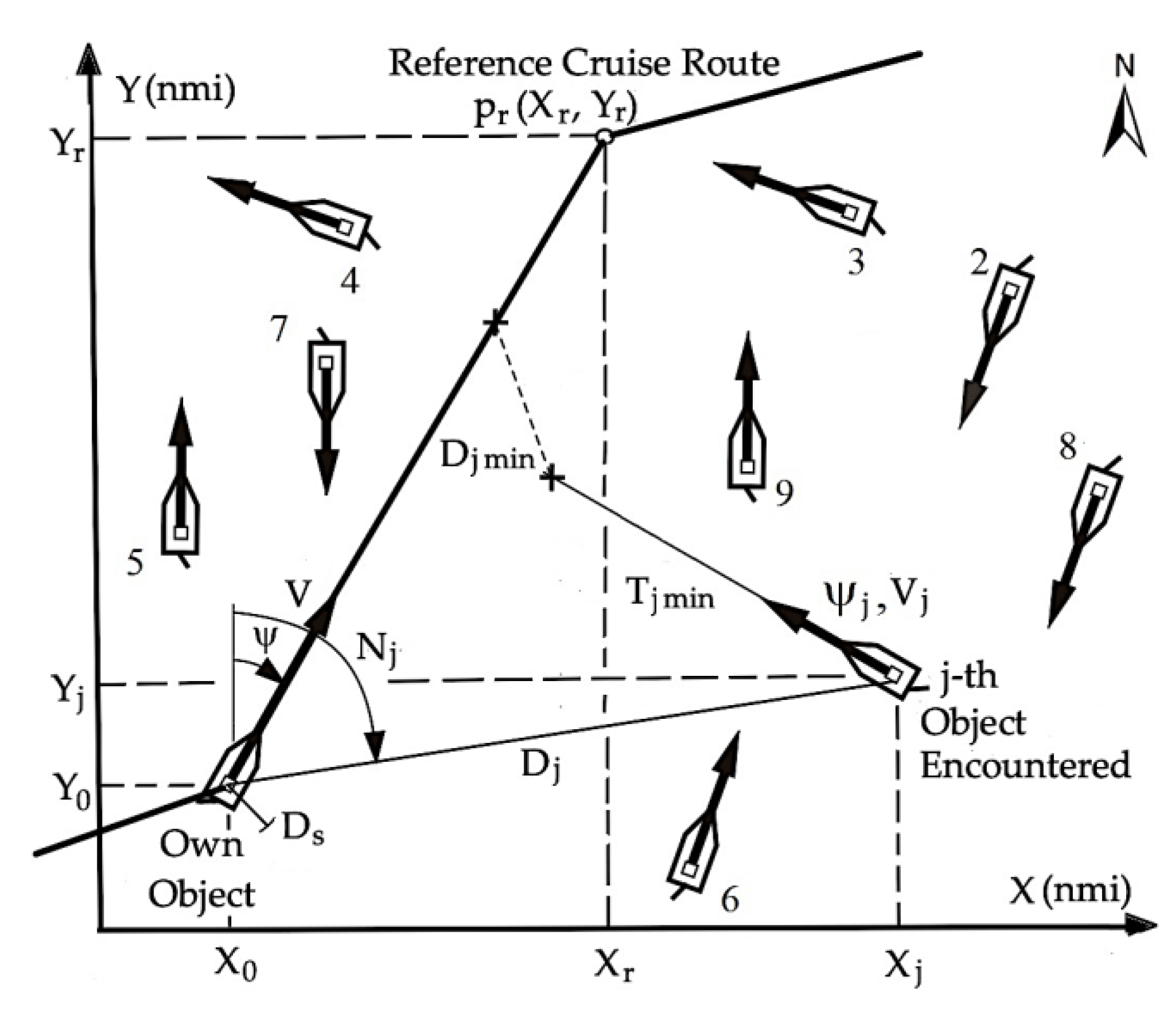
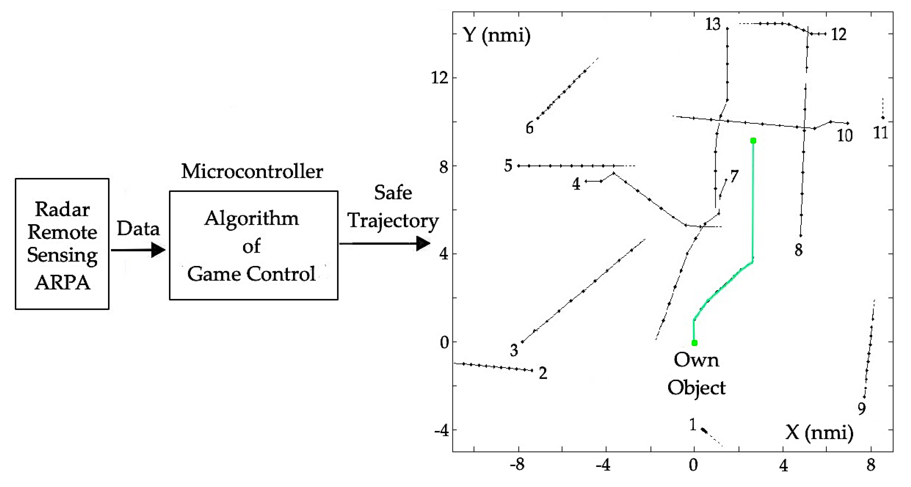
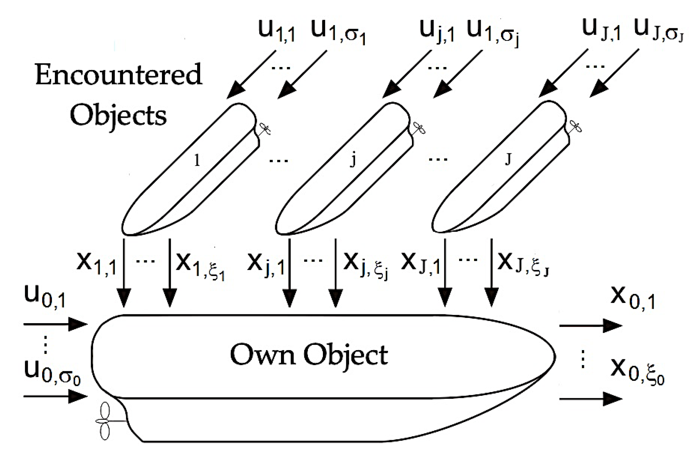
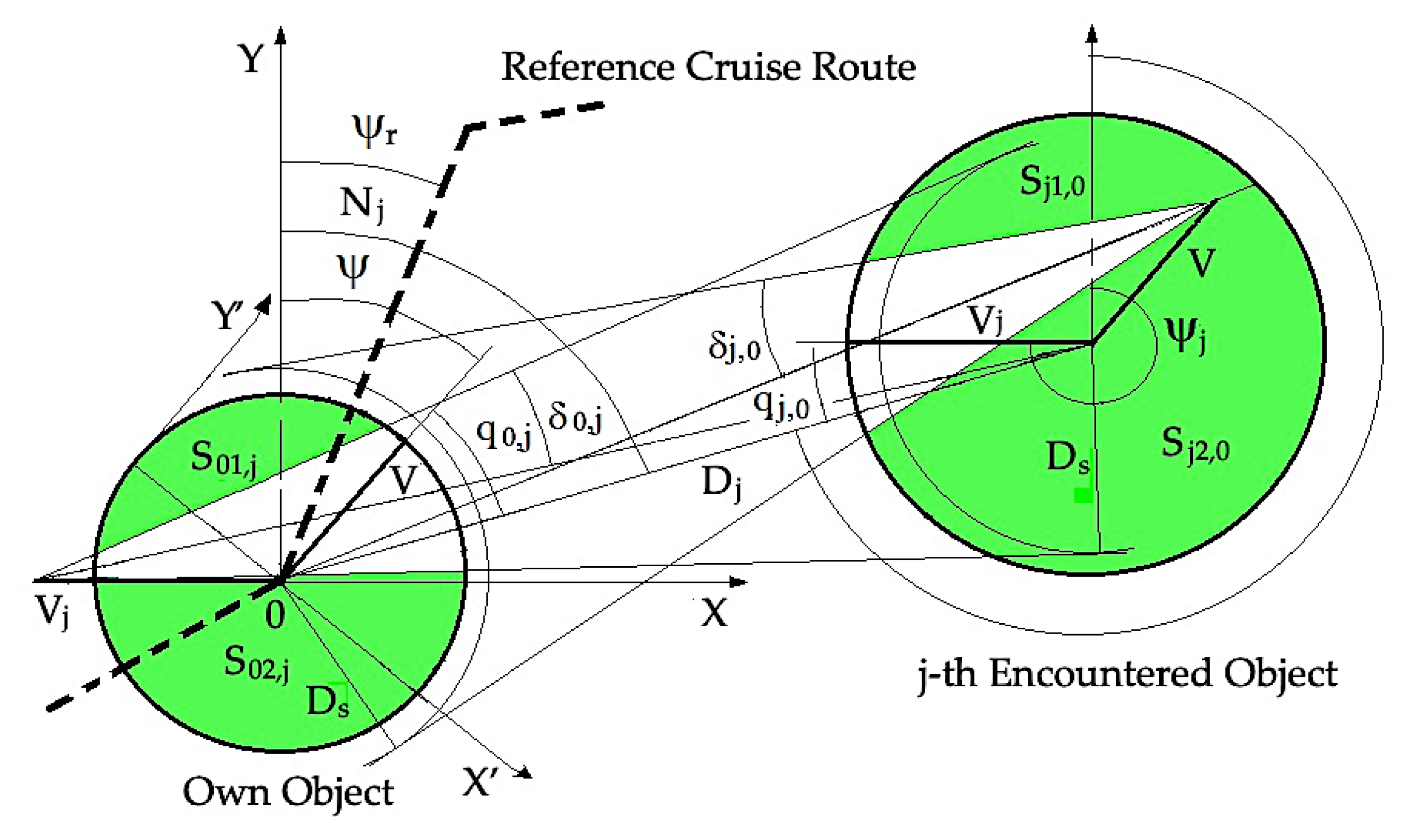
Own object, moving course ψ at speed V, is equipped with an ARPA device, performs radar remote sensing of the encountered j-th object, moving course ψj at speed Vj, at distance Dj and bearing Nj (Figure 1).
The ARPA device only allows the movement of objects to be directed to the minimum necessary extent, which is the result of the COLREGs rules, and is limited to a trial maneuver in relation to a small number of objects, where the navigator’s subjectivity in the assessment of steering decisions is highly important, often leading to collision situations. Therefore, it is advisable to supplement the ARPA system with the function of the computer-aided calculation of safe object passage because there are subsequent course and speed changes in relation to many objects that are passed (Figure 2).
The crucial part of the computer-aided navigator system, in the generation of control decisions, is the steering algorithm, which uses data from ARPA radar remote sensing and the appropriate process model, which calculates the safe trajectory of the object. In taking into account the game properties of the steering process, the most basic and adequate is the differential game model, which is most often used as a laboratory simulation model.
When designing practical real-time control algorithms, simpler surrogate models are used. Such surrogate models include the positional game model and matrix game model.
3. Basic Model of Differential Game
The COLREGs rules on transport safety mandate that all facilities must comply with and apply only to two objects, especially in good visibility at sea. In restricted visibility at sea, they are limited to very general recommendations that result from “good seagoing practice”. In situations where multiple objects pass each other in bad weather conditions, the movement of objects often occurs with the close coordination of actions and leads to the risk of conflict and collision.
Therefore, in analyzing the work by Bressan et al. and Gromova et al. [49,50], it is expedient to present the process as well as the development and testing for the operation of methods of safe control of the object using the basics of game theory. To take into account both possible object strategies to avoid collisions, as well as their movement dynamics described by differential equations, the most appropriate model is the differential game of multiple objects (Figure 3).
3.1. State Equations
By applying the work in References [51,52], the state equations of the differential game will take the following form:
and by the following detailed state equations:
Description of state and control variables is presented in Table 1.
The basic model of differential game is a generalized model of the described control process and contains measurable and non-measurable variables. We can measure all variables on our object, but not all variables of the meet object. Therefore, variables such as Hr, , and Ftj are only found in the generalized base model. Moreover, for the synthesis of practical control algorithms, we will have to simplify this generalized model and find the surrogate models presented in Section 4 to use only measurable quantities.
3.2. Limits of Control and State
The obligation to observe the safe distance between objects, formulated by the relationship (4), leads to the following restriction on the control and state of the process:
These restrictions in sea navigation are called domains that can have different shapes, for example, a circle, ellipse, hexagon, or parabola. An artificial neural network can be used to create them.
3.3. Control Criterion
As a criterion for determining the best game control out of many acceptable object strategies, the value of the so-called mathematics of game theory, integral payoff and final payoff are used:
When considering the work by Reddy et al. [53], the integral payoff of the game represents the closing of the own object path passing of j-th object and the final payoff of the game consists of the risk of collision rjf and descent εf of the own object from the set route.
3.4. Computer Simulation
In the example of a container ship with a load capacity of 15,000 DWT, the state equation (6) was modeled in MATLAB/SIMULINK software, obtaining a computer simulator of controlling its own object in situations where many objects are encountered. In this way, it becomes possible to both perform a laboratory study of various possible states of the anti-collision process and test practical algorithms for the safe control of the object.
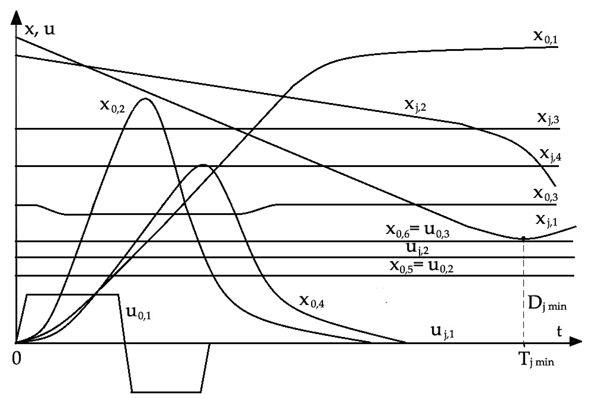
Figure 4 illustrates the nature and extent of changes in state and control variables during simulation of the basic model of the game control process during an anti-collision maneuver with a change of course.
According to References [54,55,56], the base model of the differential game is a computer tool for studying the movement of objects in collision situations and is used to test the software developed for navigator decision support. In addition to the high complexity of this model, simplified models are formulated for the design of practical computer control programs, with the simultaneous application of selected artificial intelligence methods.
4. Surrogate Models of Differential Game
4.1. Positional Game Model
Based on Nisan et al. [57], it can be assumed that the positional game model includes the dependency of own object strategy in encountered object position p(tk). However, the strategies of the encountered objects are also assigned to this position.
Thus, the coordinates of the position of the objects make up the state of the entire process of their safe passing:
4.1.1. Sets of Object Safe Strategies
Acceptable game control of the own object u0 and uj of the j-th encountered object includes the kinematics of their movement, recommendations of COLREGs sea route rules described in [58,59] and condition (4)—maintaining a safe passing distance Ds—to create sets of acceptable game positional strategies, i.e., U0,j and Uj,0:
Figure 5 shows the method used to determine the acceptable strategy areas resulting from the possibility of passing ships from the portside (PS) or starboard side (SS).
The set of own object safe strategies U0,j is described as follows:
where the individual amounts are:
The value of variable λ0,j is determined using logic function Lj, which characterizes the requirements of the COLREGs rules. This function results from the semantic interpretation of the text of COLREGs legal provisions in order to include them in the computer algorithm to control the movement of the object:
Each particular type of the situation involving the approach of the ships is assigned the logical variable value equal to one or zero:
- A—encounter of the ship from bow or from any other direction,
- B—approaching or moving away of the ship,
- C—passing the ship astern or ahead,
- D—approaching of the ship from the bow or from the stern,
By minimizing logical function Lj by using a method of the Karnaugh's Tables following is obtained:
Similar to the previous dependencies, the set of safe strategies Uj,0 for the j-th object is described as follows:
where the individual amounts are:
The safe trajectory of the own object, relative to all the J objects passed, is calculated by taking into account the following combined set of possible strategies:
4.1.2. Positional Game Control
The calculation of the optimal and safe game control of the movement of own object takes place in the following three steps:
Step 1: Sets of possible strategies for individual Uj,0 encountered objects in relation to own ship are defined, as well as initial sets of U0,j possible strategies of own object for these objects.
Step 2: The own object steering u0,j and j-th object steering uj,0 are determined, followed by the optimal positional strategy u0*[p(tk)] of own object, ensuring the control quality index I* optimal value.
Step 3a: For a non-cooperative positional game, the control quality index will take the form:
where L means the distance of own object at time t0 to turn to the position on the reference cruise route.
First of all, from the condition of min1, the control u0,j of the own object is established to ensure the shortest way of passing each j-th object. Secondly, with the max2 condition for the non-cooperative control uj,0 of each encountered object, contributing to the largest deviation of the own object trajectory. Thirdly, from the min3 condition from the total U0 of the own object control set to all encountered objects, the optimal control of own object is selected, ensuring the smallest path loss.
To calculate the optimal control of the own object, which ensures the three above-mentioned optimization conditions (min3, max2, min1), the use of the triple SIMPLEX linear programming method is proposed.
In this optimization task, the smallest deviation of the own object from a reference cruise route is matched by providing the maximum longitudinal component of the velocity vector of the own object from a possible set of strategies. The above calculations are repeated sequentially at each subsequent stage of the cruise route, obtaining optimal safe course ψ and speed V of own object.
Step 3b: For the cooperative positional game, the control quality index will take the form:
The difference from the non-cooperative game algorithm is that the max2 criterion is changed to the min2 criterion.
Computational programs of the pgnc non-cooperative positional game, according to (18), and the pgc positional cooperative game, according to (19), were implemented in the software (lp) linear programming from the Optimization Toolbox MATLAB.
4.1.3. Computer Simulation
4.2. Matrix Game Model
Replacing the differential equations of dynamic motion of objects with the appropriate maneuver advance time allows the differential game model to be brought into the surrogate matrix game model.
Then, the objects controlling their movement by means of course and speed changes, and their current state, related to traffic safety, is characterized by mutual distance Dj and bearing Nj with the radar remote sensing ARPA system and rj risk of collision.
4.2.1. Matrix of Risk Collision
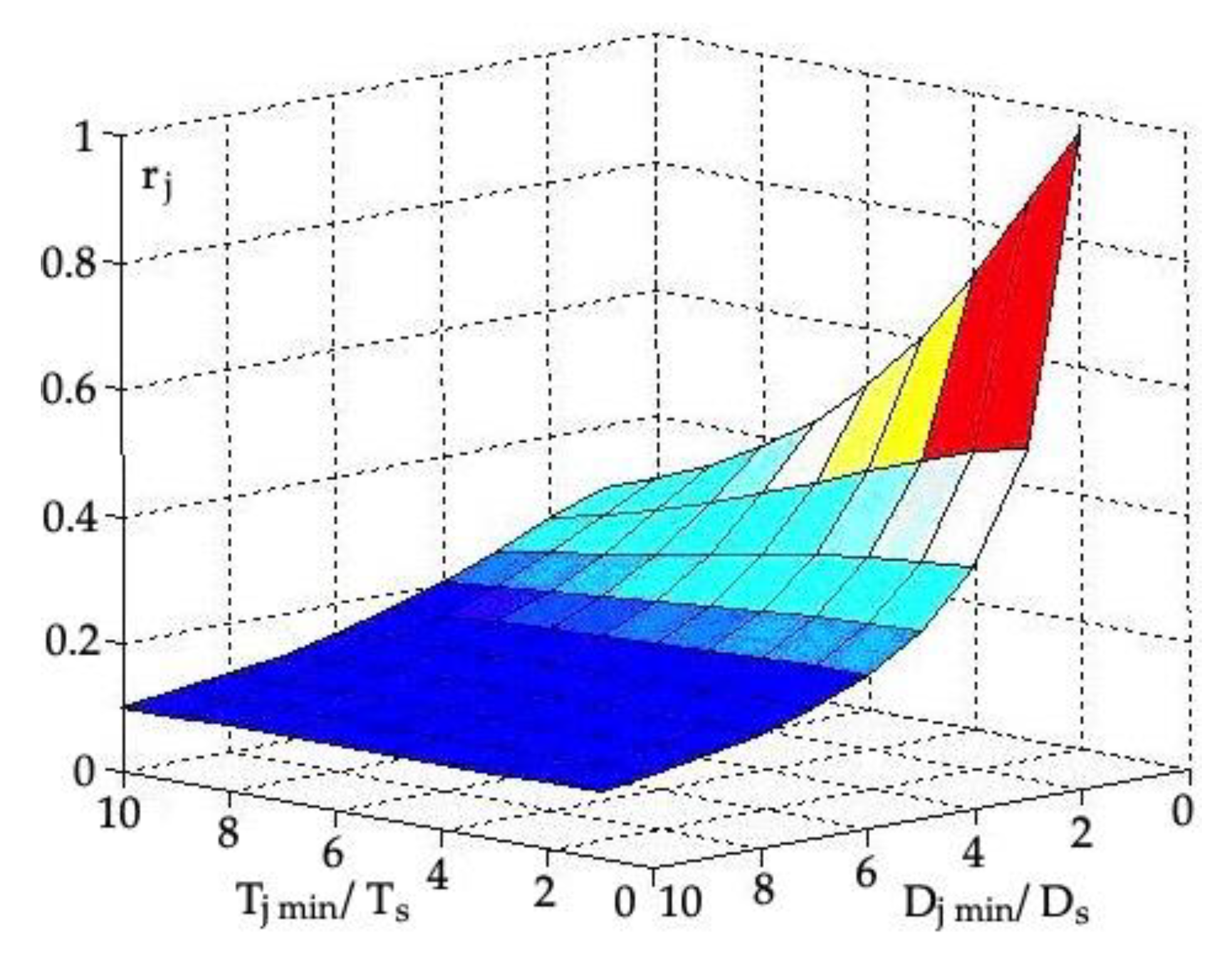
Having considered the work by Modarres [60], the author of this article proposes a new formulation of object collision risk as a reference to two assessments of the same navigational situation.
The first assessment contains the parameters Dj min and Tj min of the real situation of the proximity of the objects. The second assessment concerns the same situation, but the safety is determined by parameters Ds, Ts, and Dj.
Thus, this reference has three relative elements: Dj min/Ds, Tj min/Ts, and Dj/Ds, all of which are proposed to express the risk of collision rj(u0,uj) as the following mean square form of these three relative elements:
where the weighting factors η1, η2 and η3 assess the state of visibility at sea—good or limited type of navigation area and open or fairway (Figure 9).
Matrix game R in which player OO—own object can use u0 clean strategies, and player EO—encountered objects with uj clean strategies, which can be described using the following collision risk matrix:
The number of rows in the R matrix risk of collision is equal to the number of possible OO strategies of the player as deviations of his course or speed:
The number of columns consists of the total number of permissible strategies for all the players EO involved in a collision situation, by analogy to all the changes in the course and speed of each met object:
In addition, we need to follow the COLREG rules, which impose restrictions on the possible strategies (u0i, uji).
4.2.2. Matrix Game Control
In practice, the matrix game of many objects only uses pure strategies that do not reach the state determined by Nash [45] equilibrium points. Then, a substitute solution to such a real game is obtained by using mixed strategies that are the probabilities of pure strategies.
Step 1: The probability matrix P of using pure strategies in the game control will take the following form:
The optimal control of the own object is provided by its strategy, which has been assigned the highest probability of use:
Step 2a: The optimal and safe own object steering in the non-cooperative matrix game has the following dependence:
First, from the max1 condition, it is assumed that the j-th object control uj contributes to the largest deviation of the own object’s trajectory. Then, from the min2 condition, for these control uj, own object control u0 is assumed, providing the shortest safe way of passing each j-th object.
Step 2b: The quality control index of optimal and safe own object steering in the cooperative matrix game will take the following form:
The difference from non-cooperative game algorithm is that the max1 criterion is changed to the min1 criterion.
Computational programs of the mgnc non-cooperative matrix game, according to (26), and the mgc matrix cooperative game, according to (27), were implemented in the software (lp) linear programming from the Optimization Toolbox MATLAB.
4.2.3. Computer Simulation of the Matrix Game Model
The mgnc and mgc algorithms have been subjected to simulation tests in SIMULINK software in situation examples of own objects passing 13 other objects whose data from the radar remote sensing ARPA system is listed in Table 2. Simulation studies that reflected the movement of objects, both in good visibility at sea for Ds = 0.5 nmi (nautical miles) and in limited visibility at sea at Ds = 2.0 nmi (nautical miles), are shown in Figure 10 and Figure 11. Additionally, it should be clarified that, in the drawings, the trajectories of the objects encountered do not change due to the difficulty of presenting them based on complicated operations while determining the optimal element of risk matrix R and/or the probability matrix P.
5. Comparison of Game Object Control Methods
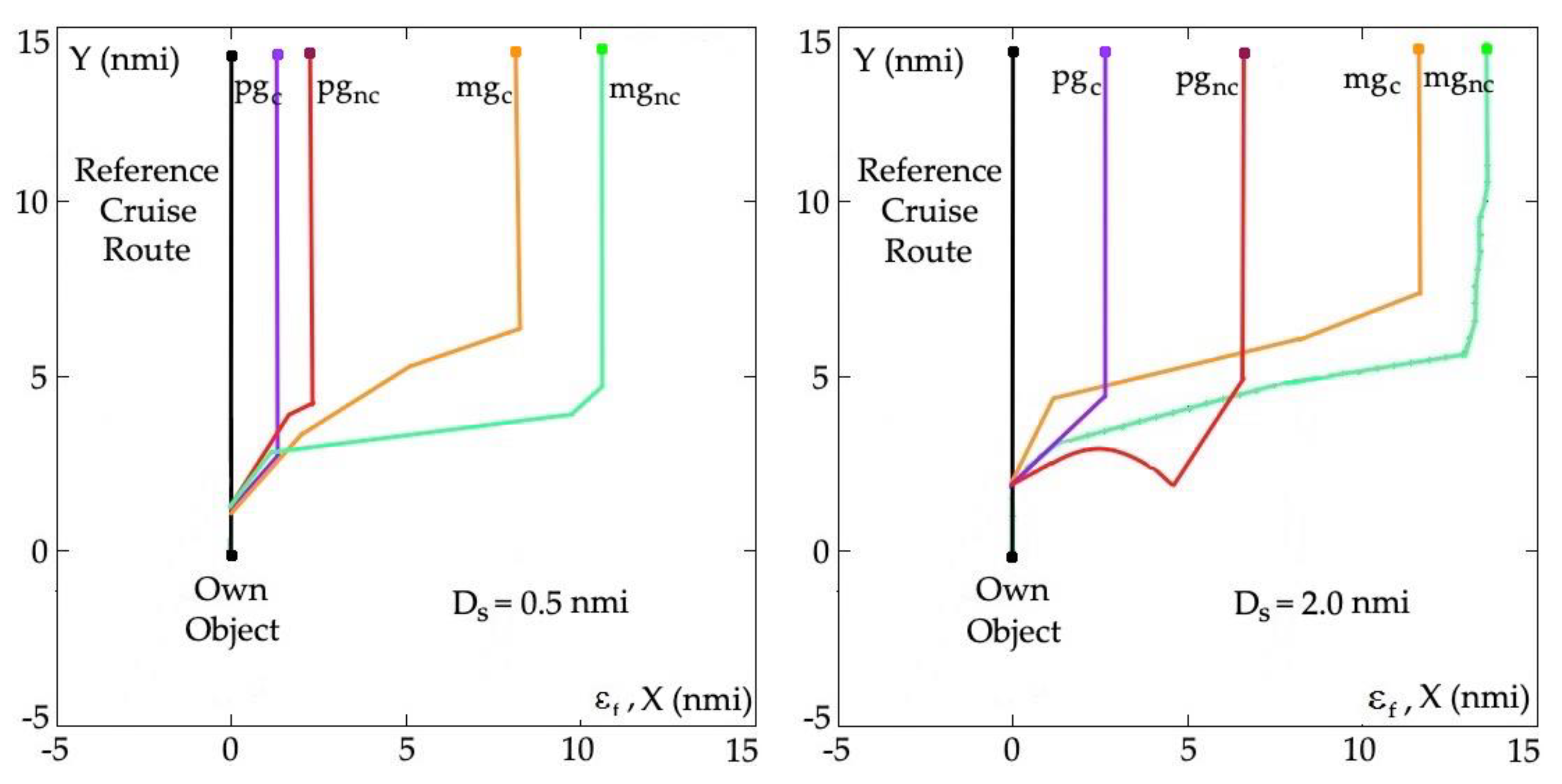
The results of computer calculations of the safe trajectory of the own object in the situation of passing by 13 encountered objects, made using developed game algorithms, are presented in Figure 12.
The deviation of the safe trajectory from its initial direction, with good visibility at sea, ranges from 0.7 nmi for a cooperative positional game, to 9.2 nmi for a non-cooperative matrix game. However, this is a deviation from the trajectory in limited visibility at sea, which ranges from 2.7 nmi for a cooperative positional game to 13.8 nmi for a non-cooperative matrix game.
6. Conclusions
An analysis of the causes of collision of objects at sea, especially in situations where multiple objects pass each other and in limited visibility at sea, indicates the importance of the navigator’s subjectivity in making steering decisions, often leading to conflict situations. Game theory comes to the rescue as a theory of resolving these conflict situations. This approach allows for the development of a more adequate model of the anti-collision process, in the form of a multi-object differential game method.
The differential game method, as a very accurate multidimensional process model, is most useful as a laboratory simulation model for the synthesis and research of practical quarterback control algorithms. For the design of such algorithms, surrogate models using positional and matrix methods, which perform a computer-assisted navigator role and significantly accelerate in making optimal and safe decisions, are the best suited.
These algorithms take into account both the COLREG rules when starting the game and the dynamics of the objects in the form of the maneuver advance time, their degree of cooperation, and the end game if the risk of collision becomes zero.
The essence of the article is to use elements of game theory to consider navigator subjectivity in collision situations and surrogate game models as positional and matrix games in the design of the entire calculation steering algorithms. A new definition of object collision risk was also presented as a reference to two assessments of the same navigational situation: the real situation of the proximity of objects and the safe situation determined by the reference parameters.
However, the designated set-up trajectories consist of consecutive maneuvers, major course changes, the smoothness of the calculated object path is important, to which the works of Hu et al. [61], Campbell et al. [62], and in particular Ravankar et al. [63] are devoted.
This work did not exhaust all the issues related to safe steering of objects at sea. In future projects, consideration of safe object steering sensitivity analysis to the data inaccuracy of ARPA radar remote sensing system, changes in object kinematics and dynamics parameters, and the impact of outside disturbances could be included.
The article deals with the deterministic approach to the problems of games and their application to control multiple moving objects. In the next works, one can consider elements of the theory of stochastic games and the possibilities of their application. Statistical evaluation of the proposed methods would also be important by simulation testing of typical navigation scenarios, for example on the ARPA simulator.
Funding
This research was funded by a research project of Gdynia Maritime University in Poland, No. WE/2020/PZ/02: “Methods of static and dynamic optimization of ship movement control.”
Conflicts of Interest
The author declares no conflict of interest.
References
- Bist, D.S. Safety and Security at Sea. In A Guide to Safer Voyages; Butter Heinemann: Oxford, UK, 2000; ISBN 0-75064-774-4. [Google Scholar]
- Cahill, R.A. Collisions and Their Causes; The Nautical Institute: London, UK, 2002; ISBN 1-87077-60-1. [Google Scholar]
- Tam, C.; Bucknall, R.; Greig, A. Review of Collision Avoidance and Path Planning Methods for Ships in Close Range Encounters. J. Navig. 2009, 62, 455–476. [Google Scholar] [CrossRef]
- Huang, Y.; Chen, L.; Chen, P.; Negenborn, R.R.; van Gelder, P.H.A.J.M. Ship Collision Avoidance Methods: State-of-the-art. Saf. Sci. 2020, 121, 451–473. [Google Scholar] [CrossRef]
- Kulakov, M.A.; Korh, M.V. Choice of Optimum Maneuver of Divergence by the Regions of Impermissible Values of Parameters. Sci. Educ. New Dimens. 2020, 27, 1–3. [Google Scholar] [CrossRef]
- Johansen, T.A.; Perez, T.; Cristofaro, A. Ship Collision Avoidance and COLREGs Compliance using Simulation-based Control Behavior Selection with Predictive Hazard Assessment. IEEE Trans. Intell. Transp. Syst. 2016, 17, 1–16. [Google Scholar] [CrossRef] [Green Version]
- Melhaoui, Y.; Ait Allal, A.; Kamil, A.; Mansouri, K.; Rachik, M. Toward an overview of ship collision avoidance maneuvers approaches in compliance with COLREG convention. In Proceedings of the IEEE 5th International Conference on Optimization and Applications, Kenitra, Morocco, 25–26 April 2019. [Google Scholar] [CrossRef]
- Kuwata, Y.; Wolf, M.; Zarzhitsky, D.; Huntsberger, T.L. Safe maritime autonomous navigation with COLREGS, using velocity obstacles. IEEE J. Ocean. Eng. 2014, 39, 110–119. [Google Scholar] [CrossRef]
- Miele, A.; Wang, T. Optimal trajectories and guidance schemes for ship collision avoidance. J. Optim. Theory Appl. 2006, 129, 1–21. [Google Scholar] [CrossRef]
- Statheros, T.; Howells, G.; Maier, K.M. Autonomous ship collision avoidance navigation concepts, technologies and techniques. J. Navig. 2008, 61, 129–142. [Google Scholar] [CrossRef] [Green Version]
- You, Y.-J.; Rhee, K.-P.; Ahn, J.-H. A method of inferring collision ratio based on maneuverability of own ship under critical collision conditions. Int. J. Nav. Archit. Ocean Eng. 2013, 5, 188–198. [Google Scholar] [CrossRef] [Green Version]
- Perera, L.P.; Carvalho, J.P.; Soares, C.G. Bayesian Network based sequential collision avoidance action execution for an Ocean Navigational System. In Proceedings of the 8th IFAC Conference on Control Applications in Marine Systems, Rostock, Germany, 15–17 September 2010; pp. 266–271. [Google Scholar] [CrossRef]
- Liu, Z.; Wu, Z.; Zheng, Z. A novel framework for regional collision risk identification based on AIS data. Appl. Ocean. Res. 2019, 89, 261–272. [Google Scholar] [CrossRef]
- Park, J.; Han, J.; Kim, J.; Son, N. Probabilistic quantification of ship collision risk considering trajectory uncertainties. IFAC-PapersOnLine 2016, 49, 109–114. [Google Scholar] [CrossRef]
- Blaich, M.; Kohler, S.; Reuter, S.; Hahn, A. Probabilistic Collision Avoidance for Vessels. IFAC-PapersOnLine 2015, 48, 69–74. [Google Scholar] [CrossRef]
- Lazarowska, A. Safe Ship Trajectory Planning Based on the Ant Algorithm—The Development of the Method. Act. Navig. Mar. Navig. Saf. Sea Transp. 2015, 153–160. [Google Scholar] [CrossRef]
- Tomera, M. Ant Colony Optimization Algorithm Applied to Ship Steering Control. 18th Annual International Conference on Knowledge-Based and Intelligent Information and Engineering Systems KES, Gdynia, Poland. Procedia Comput. Sci. 2014, 35, 83–92. [Google Scholar] [CrossRef] [Green Version]
- Ahn, J.-H.; Rhee, K.-P.; You, Y.-J. A study on the collision avoidance of a ship using neural networks and fuzzy logic. Appl. Ocean. Res. 2012, 37, 162–173. [Google Scholar] [CrossRef]
- Geng, X.; Wang, Y.; Wang, P.; Zhang, B. Motion of maritime autonomous surface ships by dynamic programming for collision avoidance and speed optimization. Sensors 2019, 19, 434. [Google Scholar] [CrossRef] [Green Version]
- Lebkowski, A. Evolutionary methods in the management of vessel traffic. In Proceedings of the International Conference on Marine Navigation and Safety of Sea Transportation, Gdynia, Poland, 17–19 June 2015; pp. 259–266. [Google Scholar]
- Dinh, G.H.; Im, N.K. Study on the Construction of Stage Discrimination Model and Consecutive Waypoints Generation Method for Ship’s Automatic Avoiding Action. Int. J. Fuzzy Log. Intell. Syst. 2017, 17, 294–306. [Google Scholar] [CrossRef] [Green Version]
- Lyu, H.; Yin, Y. COLREGS-Constrained Real-time Path Planning for Autonomous Ships Using Modified Artificial Potential Fields. J. Navig. 2019, 72, 588–608. [Google Scholar] [CrossRef]
- Hwang, J.I.; Chae, S.H.; Kim, D.; Jung, H.S. Application of Artificial Neural Networks to Ship Detection from X-Band Kompsat-5 Imagery. Appl. Sci. 2017, 7, 961. [Google Scholar] [CrossRef]
- Kang, M.; Ji, K.; Leng, X.; Lin, Z. Contextual Region-Based Convolutional Neural Network with Multilayer Fusion for SAR Ship Detection. Remote Sens. 2017, 9, 860. [Google Scholar] [CrossRef] [Green Version]
- Collingwood, A.; Treitz, P.; Charbonneau, F.; Atkinson, D.M. Artificial Neural Network Modeling of High Arctic Phytomass Using Synthetic Aperture Radar and Multispectral Data. Remote Sens. 2014, 6, 2134–2153. [Google Scholar] [CrossRef] [Green Version]
- Hertz, J.; Krogh, A.; Palmer, R.G. Introduction to the Theory of Neural Computation; CRC Press: Boca Raton, FL, USA, 2018; ISBN 978-0-201-51560-1. [Google Scholar]
- Hinostroza, M.A.; Xu, H.; Soares, C.G. Cooperative operation of autonomous surface vehicles for maintaining formation in complex marine environment. Ocean Eng. 2019, 183, 132–154. [Google Scholar] [CrossRef]
- Liu, Z.; Wu, Z.; Zheng, Z. A cooperative game approach for assessing the collision risk in multi-vessel encountering. Ocean Eng. 2019, 187, 106175. [Google Scholar] [CrossRef]
- Hagen, I.B.; Kufoalor, K.M.; Brekke, E.F.; Johansen, T.A. MPC-based collision avoidance strategy for existing marine vessel guidance systems. In Proceedings of the IEEE International Conference on Robotics and Automation, Brisbane, Australia, 21–25 May 2018. [Google Scholar] [CrossRef]
- Chen, Y.; Georgiou, T.T.; Pavon, M. Covariance steering in zero-sum linear-quadratic two-player differential games. arXiv 2019, arXiv:1909.05468v1. [Google Scholar]
- Gronbaek, L.; Lindroos, M.; Munro, G.; Pintassilgo, P. Cooperative Games in Fisheries with More than Two Players. In Game Theory and Fisheries Management; Springer: Cham, Switzerland, 2020; pp. 81–105. ISBN 978-3-030-40112-2. [Google Scholar]
- Isaacs, R. Differential Games; John Wiley & Sons: New York, NY, USA, 1965; ISBN 0-48640-682-2. [Google Scholar]
- Gluver, H.; Olsen, D. Ship Collision Analysis; August Aimé Balkema: Rotterdam, The Netherlands, 1998; ISBN 90-5410-962-9. [Google Scholar]
- Perera, L.P.; Carvalho, J.P.; Soares, C.G. Autonomous guidance and navigation based on the COLREGs rules and regulations of collision avoidance. In Proceedings of the International Workshop “Avoidance Ship Design for Pollution Prevention”, Split, Croatia, 23–24 November 2009; pp. 1–12. [Google Scholar] [CrossRef]
- Sadler, D.H. The mathematics of collision avoidance at sea. J. Navig. 2010, 10, 306–319. [Google Scholar] [CrossRef]
- Dockner, E.; Feichtinger, G.; Mehlmann, A. Noncooperative solutions for a differential game model of the fishery. J. Econ. Dyn. Control. 1989, 13, 1–20. [Google Scholar] [CrossRef]
- Baba, N.; Jain, L.C. Computational Intelligence in Games; Physica-Verlag: Heidelberg, Germany, 2001; ISBN 978-3-662-00369-5. [Google Scholar]
- Breton, M.; Szajowski, K. Advances in Dynamic Games: Theory, Applications and Numerical Methods for Differential and Stochastic Games; Birkhauser: Boston, MA, USA, 2010; ISBN 978-0-8176-8089-3. [Google Scholar]
- Sanchez-Soriano, J. An overview of game theory applications to engineering. Int. Game Theory Rev. 2013, 15, 1–18. [Google Scholar] [CrossRef]
- Haurie, A.; Krawczyk, J.B.; Zaccour, G. Games and Dynamic Games, Subtle Connections; University Press: Cambridge, UK, 2012; ISBN 978-9814401265. [Google Scholar]
- Mesterton-Gibbons, M. An. Introduction to Game Theoretic Modelling; American Mathematical Society: Providence, RI, USA, 2001; ISBN 978-0-82-181929-6. [Google Scholar]
- Osborne, M.J. An. Introduction to Game Theory; Oxford University Press: New York, NY, USA, 2004; ISBN 978-0-19512895-6. [Google Scholar]
- Broek, W.A.; Engwerda, J.C.; Schumacher, J.M. Robust equilibria in indefinite linear-quadratic differential games. J. Optim. Theory Appl. 2003, 119, 565–595. [Google Scholar] [CrossRef]
- Basar, T.; Olsder, G.J. Dynamic Non-Cooperative Game Theory; SIAM: Philadelphia, PA, USA, 1998; ISBN 978-0-898-714-29-6. [Google Scholar]
- Nash, J.F. Non-cooperative games. Ann. Math. 1951, 54, 286–295. [Google Scholar] [CrossRef]
- Miloh, T. Determination of Critical Maneuvres for Collision Avoidance Using the Theory of Differential Games; Bericht: Hamburg, Germany, 1975; ISBN 10.15480/882.666. [Google Scholar]
- Olsder, G.J.; Walter, J.L. A Differential Game Approach to Collision Avoidance of Ships. Optim. Technol. 1977, 6, 264–271. [Google Scholar]
- Wells, D. Games and Mathematics; Cambridge University Press: Cambridge, UK, 2013; ISBN 978-1-107-02460-1. [Google Scholar]
- Bressan, A.; Nguyen, K.T. Stability of feedback solutions for infinite horizon noncooperative differential games. Dyn. Games Appl. 2018, 8, 42–78. [Google Scholar] [CrossRef]
- Gromova, E.V.; Petrosyan, L.A. On an approach to constructing a characteristic function in cooperative differential games. Autom. Remote Control. 2017, 78, 1680–1692. [Google Scholar] [CrossRef]
- Kun, G. Stabilizability, Controllability, and Optimal Strategies of Linear and Nonlinear Dynamical Games. Ph.D. Thesis, RWTH Aachen, Beijing, China, 2001. [Google Scholar]
- Perez, T. Ship Motion Control; Springer: Berlin/Heidelberg, Germany, 2005; ISBN 978-1-84628-157-0. [Google Scholar]
- Reddy, P.V.; Zaccour, G. Feedback Nash equilibria in linear-quadratic difference games with constraints. IEEE Trans. Autom. Control. 2016, 62, 590–604. [Google Scholar] [CrossRef]
- Basar, T.; Bernhard, P. H-Infinity Optimal Control and Related Mini-Max Design Problems: A Dynamic Game Approach; Birkhauser: Boston, MA, USA, 2008; ISBN 978-0-8176-4757-5. [Google Scholar]
- Engwerda, J.C. LQ Dynamic Optimization and Differential Games; John Wiley & Sons: West Sussex, UK, 2005; ISBN 978-0-470-01524-7. [Google Scholar]
- Millington, I.; Funge, J. Artificial Intelligence for Games; Elsevier: Burlington, MA, USA, 2009; ISBN 978-0-12-374731-0. [Google Scholar]
- Nisan, N.; Roughgarden, T.; Tardos, E.; Vazirani, V. Algorithmic Game Theory; Cambridge University Press: Cambridge, UK, 2007; ISBN 978-0-521-87282-9. [Google Scholar]
- Cockcroft, C.; Lameijer, J. A Guide to the Collision Avoidance Rules; Butterworth-Heinemann Publication: Oxford, UK, 2012; ISBN 978-0-080-97170-4. [Google Scholar]
- COLREGs Course. Available online: https://ecolregs.com/index.php?option=com_k2&view=item&layout=item&id=51&Itemid=383&lang=en (accessed on 15 February 2020).
- Modarres, M. Risk Analysis in Engineering, Techniques, Tools and Trends; Taylor & Francis: Boca Raton, FL, USA, 2006; ISBN 1-574444-794-7. [Google Scholar]
- Hu, L.; Naeem, W.; Rajabally, E.; Watson, G.; Mills, T.; Bhuiyan, Z.; Raeburn, C.; Salter, I.; Pekcan, C. A multi-objective optimization approach for COLREGs-compliant path planning of autonomous surface vehicles verified on networked bridge simulators. IEEE Trans. Intell. Transp. Syst. 2020, 21, 1167–1179. [Google Scholar] [CrossRef] [Green Version]
- Campbell, S.; Naeem, W. A rule-based heuristic method for COLREGs-compliant collision avoidance for an unmanned surface vehicle. IFAC Proc. Vol. 2012, 45, 386–391. [Google Scholar] [CrossRef]
- Ravankar, A.; Ravankar, A.A.; Kobayashi, Y.; Hoshino, Y.; Peng, C.C. Path smoothing techniques in robot navigation: State-of-art, current and future challenges. Sensors 2018, 18, 3170. [Google Scholar] [CrossRef] [Green Version]
Figure 1.
Displaying the situation of passing own object with multiple objects, in particular with the j-th object: X0, Y0—own object coordinates; Xj, Yj—j-th object coordinates; Xr, Yr—own object reference coordinates; pr—the reference position of own object; Dj min—distance of the closest point of approach; Tj min—time to the closest point of approach; and Ds—a safe distance of approach.

Figure 2.
The system of computer-aided object safe control.

Figure 3.
Interaction of the movement of own object and multiple passing objects: u0, x0—control and state of the own object; and uj, xj—control and state of the j-th object.
Figure 3.
Interaction of the movement of own object and multiple passing objects: u0, x0—control and state of the own object; and uj, xj—control and state of the j-th object.

Figure 4.
Runs of state and control variables of the differential game model during the anti-collision maneuver of changing the course of own object.
Figure 4.
Runs of state and control variables of the differential game model during the anti-collision maneuver of changing the course of own object.

Figure 5.
Graphic design of acceptable sets of strategies for own object: U0,j = S01,j or S02,j and for j-th encountered object: Uj,0 = Sj1,0 or Sj2,0.
Figure 5.
Graphic design of acceptable sets of strategies for own object: U0,j = S01,j or S02,j and for j-th encountered object: Uj,0 = Sj1,0 or Sj2,0.

Figure 6.
Displaying a computer simulated situation of the own object passing 13 objects encountered in the form of 12-minute velocity vectors.
Figure 6.
Displaying a computer simulated situation of the own object passing 13 objects encountered in the form of 12-minute velocity vectors.

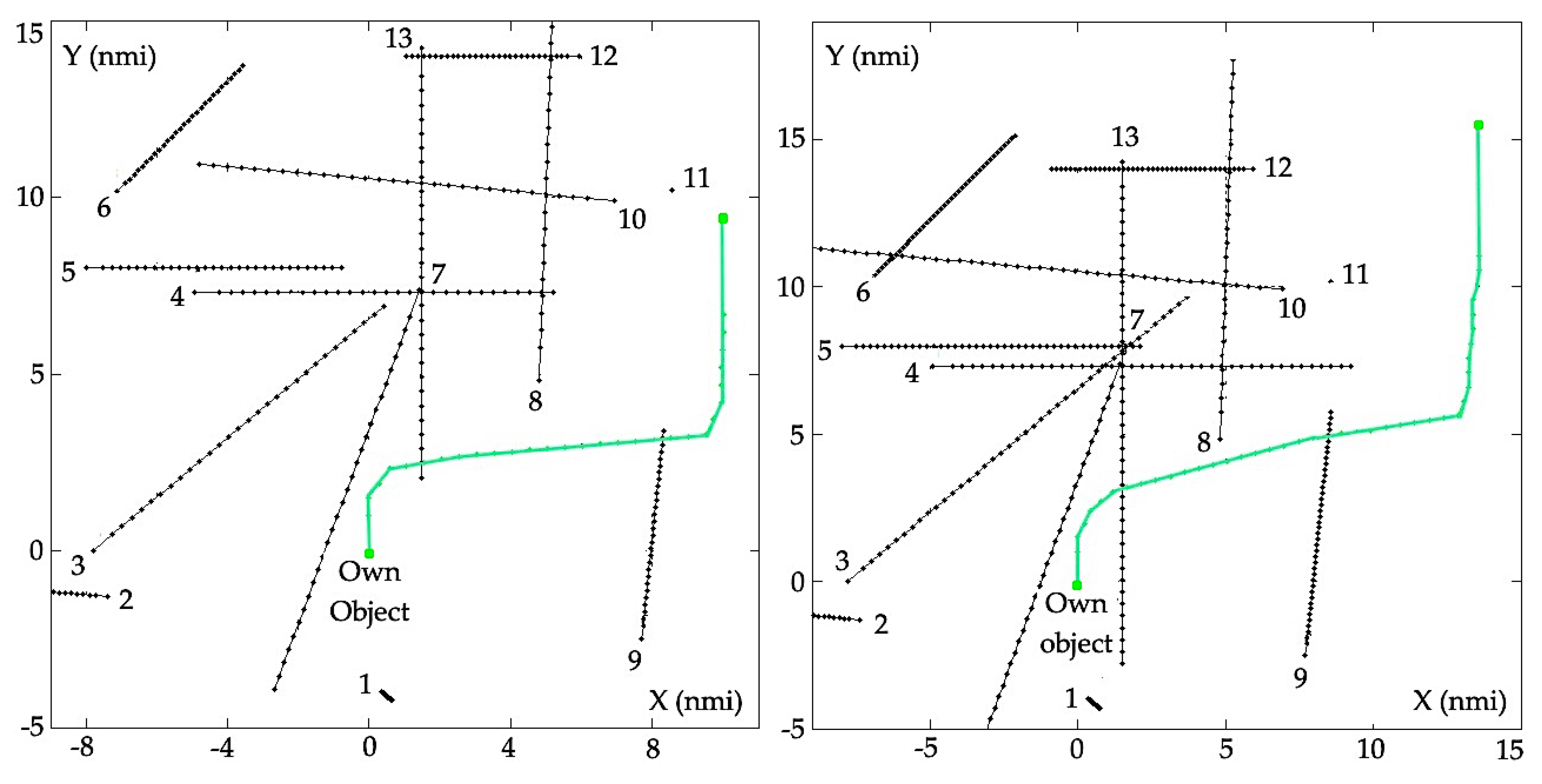
Figure 7.
Object game trajectories calculated according to the pgnc algorithm of the non-cooperative positional game control: on the left—with good visibility at sea, with the final payoff of the game εf = 1.3 nmi achieved, assessing the deviation safe trajectory from reference cruise route; on the right—with limited visibility at sea, with the final payoff of the game εf = 5.8 nmi.

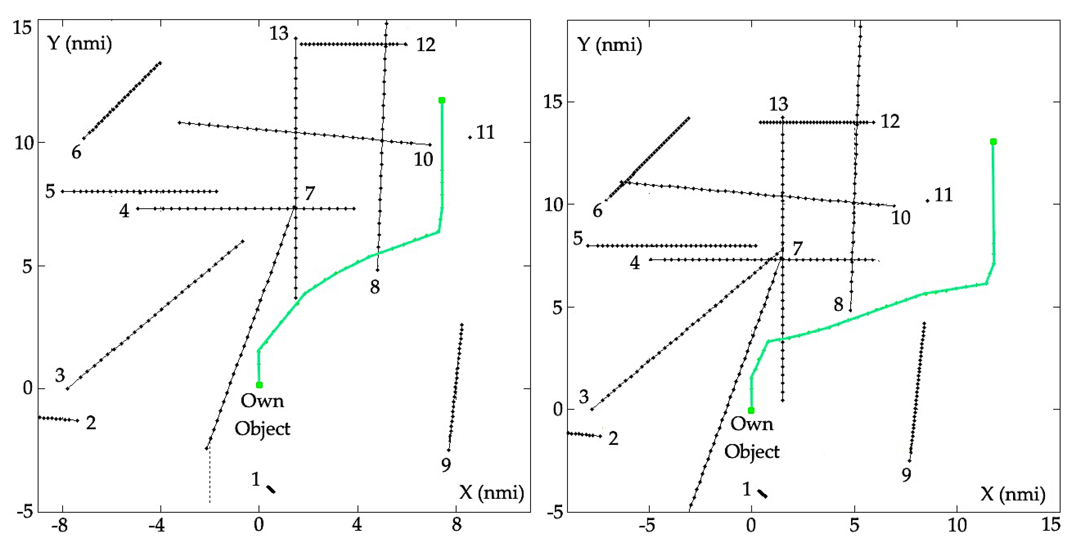
Figure 8.
Object game trajectories calculated according to the pgc algorithm of the cooperative positional game control: on the left—with good visibility at sea, with the final payoff of the game εf = 0.7 nmi achieved, assessing the deviation safe trajectory from reference cruise route; on the right—with limited visibility at sea, with the final payoff of the game εf = 2.7 nmi.

Figure 9.
Collision risk dependence of relative distance and time values of passing objects.

Figure 10.
Object game trajectories calculated according to the mgnc algorithm of non-cooperative matrix game control: on the left—with good visibility at sea, with the final payoff of the game εf = 9.2 nmi achieved, assessing deviation safe trajectory from reference cruise route; on the right—with limited visibility at sea, with the final payoff of the game εf = 13.8 nmi.

Figure 11.
Object game trajectories calculated according to the mgc algorithm of cooperative matrix game control: on the left—with good visibility at sea, with the final payoff of the game εf = 7.4 nmi achieved, assessing deviation safe trajectory from reference cruise route; on the right—with limited visibility at sea, with the final payoff of the game εf = 12.1 nmi.

Figure 12.
Safe trajectories of the own object during good visibility at sea at Ds = 0.5 nmi (left) and in limited visibility at sea at Ds = 2.0 nmi (right) calculated using the following algorithms: pgc—cooperative positional game, pgnc—non-cooperative positional game, mgc—cooperative matrix game, mgnc—non-cooperative matrix game; and εf—deviation of safe trajectory from reference cruise route.


Table 1.
Description of state and control variables.
| Variable | Means | Symbol |
|---|---|---|
| own object state ξ0—dimensional vector | ||
| x0,1 | own object course | ψ |
| x0,2 | angular speed of the own object of return | |
| x0,3 | own object speed | V |
| x0,4 | own object drift angle | β |
| x0,5 | own object main drive screw rotational speed | n |
| x0,6 | own object main drive propeller pitch | H |
| j-th object state ξj—dimensional vector | ||
| xj,1 | distance to the j-th object | Dj |
| xj,2 | bearing to the j-th object | Nj |
| xj,3 | course of the j-th object | ψj |
| xj,4 | speed of the j-th object | Vj |
| own object control σ0 - dimensional vector | ||
| u0,1 | own object rudder deflection reference angle | αr |
| u0,2 | own object main propeller reference rotational speed | nr |
| u0,3 | own object main drive screw reference stroke | Hr |
| j-th object control σj—dimensional vector | ||
| uj,1 | angular speed of the j-th object of return | |
| uj,2 | thrust force of the propeller of the j-th object | Ftj |
Table 2.
Data of the own object and 13 encountered objects.
| Bearing Nj (o) | DistanceDj (nmi) | Speed Vj (kn) | Course ψj (o) | |
|---|---|---|---|---|
| Own Object | - | - | 20 | 0 |
| Object 1 | 175 | 4.0 | 0.5 | 130 |
| Object 2 | 260 | 7.5 | 6.9 | 275 |
| Object 3 | 270 | 7.8 | 14.3 | 50 |
| Object 4 | 315 | 11.3 | 9.6 | 90 |
| Object 5 | 326 | 8.8 | 13.5 | 90 |
| Object 6 | 325 | 12.4 | 6.7 | 45 |
| Object 7 | 11 | 7.5 | 16.0 | 200 |
| Object 8 | 45 | 6.8 | 19.1 | 2 |
| Object 9 | 108 | 8.1 | 7.9 | 6 |
| Object 10 | 35 | 12.1 | 15.7 | 275 |
| Object 11 | 40 | 13.3 | 0 | 0 |
| Object 12 | 23 | 15.2 | 6.5 | 270 |
| Object 13 | 6 | 14.3 | 16.2 | 180 |
© 2020 by the author. Licensee MDPI, Basel, Switzerland. This article is an open access article distributed under the terms and conditions of the Creative Commons Attribution (CC BY) license (http://creativecommons.org/licenses/by/4.0/).
Share and Cite
MDPI and ACS Style
Lisowski, J. Game Control Methods Comparison when Avoiding Collisions with Multiple Objects Using Radar Remote Sensing. Remote Sens. 2020, 12, 1573. https://doi.org/10.3390/rs12101573
AMA Style
Lisowski J. Game Control Methods Comparison when Avoiding Collisions with Multiple Objects Using Radar Remote Sensing. Remote Sensing. 2020; 12(10):1573. https://doi.org/10.3390/rs12101573
Chicago/Turabian StyleLisowski, Józef. 2020. "Game Control Methods Comparison when Avoiding Collisions with Multiple Objects Using Radar Remote Sensing" Remote Sensing 12, no. 10: 1573. https://doi.org/10.3390/rs12101573
Note that from the first issue of 2016, this journal uses article numbers instead of page numbers. See further details here.