Satellite-Observed Soil Moisture as an Indicator of Wildfire Risk


Department of Geography, Environment and Geomatics, University of Guelph, Guelph, ON N1G 2W1, Canada
*
Author to whom correspondence should be addressed.
Remote Sens. 2020, 12(10), 1543; https://doi.org/10.3390/rs12101543
Submission received: 20 February 2020
/
Revised: 6 May 2020
/
Accepted: 7 May 2020
/
Published: 12 May 2020
(This article belongs to the Section Remote Sensing in Agriculture and Vegetation)
Abstract
:Wildfires are a concerning issue in Canada due to their immediate impact on people’s lives, local economy, climate, and environment. Studies have shown that the number of wildfires and affected areas in Canada has increased during recent decades and is a result of a warming and drying climate. Therefore, identifying potential wildfire risk areas is increasingly an important aspect of wildfire management. The purpose of this study is to investigate if remotely sensed soil moisture products from the Soil Moisture and Ocean Salinity (SMOS) satellite can be used to identify potential wildfire risk areas for better wildfire management. We used the National Fire Database (NFDB) fire points and polygons to group the wildfires according to ecozone classifications, as well as to analyze the SMOS soil moisture data over the wildfire areas, between 2010–2017, across fourteen ecozones in Canada. Timeseries of 3-day, 5-day, and 7-day soil moisture anomalies prior to the onset of each wildfire occurrence were examined over the ecozones individually. Overall, the results suggest, despite the coarse-resolution, SMOS soil moisture products are potentially useful in identifying soil moisture anomalies where wildfire hot-spots may occur.
1. Introduction
Wildfires are considered to be a natural disturbance to terrestrial ecosystems, as well as an integral part of ecosystems’ natural evolution. However, large wildfires, particularly when due to human activity, can be considered hazardous to ecosystems as they interrupt an ecosystem’s natural evolution. Nevertheless, whether it is natural or human induced, large wildfires significantly affect regional climate, the land surface hydrology, biogeochemical processes, and wildlife habitats, as well as the livelihoods of people. Recent studies have attributed the increase of large wildfire occurrences to a warming climate due to increased greenhouse effect [1,2,3,4]. The warming trend is expected to continue in the coming decades, potentially increasing the vulnerability of ecosystems to wildfires and related climate disturbances [5].
The increase in vulnerability of ecosystems to wildfires in a warming climate is of great concern to Canada since the country holds some of the largest forest ecozones in the world. For example, the Boreal Shield, being the largest ecozone in Canada, covers almost 20% of the total landmass, accounting for the majority of recorded wildfire area burned annually across Canada. On average, approximately two million hectares of forests are subject to fire annually across Canada [6,7]. The total carbon emission from these wildfires is estimated at 27 Tg carbon per year [6,8,9,10,11,12]. Within Canada, managed forests, which are subjected to more intensive fire suppression measures than unmanaged forests, are primarily located in the southern extent of the country, while the majority of unmanaged forests are located away from population centers [13]. Given the risks involved in managing large wildfires, identifying potential wildfire risk areas or “hot-spots” in advance is one of the most important aspect of wildfire management [14,15]. Several studies have stressed the need to develop methods to detect potential hot-spots in advance to minimize wildfire related damages and manage firefighting resources [16].
Remote sensing has emerged as a leading tool for forest surveys, large-scale active wildfire monitoring, and for surveying the aftermath of wildfires [17,18,19]. Several studies have shown the effectiveness of using remote sensing data in operational fire weather forecast and warning systems around the world, such as the National Fire Danger Rating System (NFDRS) in the United States [20] and the Canadian Forest Fire Danger Rating System (CFFDRS) in Canada [21,22,23,24]. These early warning systems rely primarily on remotely sensed vegetation information and important meteorological parameters, such as wind, precipitation, air temperature, and humidity.
Among hydrological variables that play a role in the occurrence of wildfire, soil moisture (SM) is of particular value. For example, SM when interpreted to also reflect the moisture of duff layers, represents the wetness state of the available fuel [25]. Another important property of SM is its temporal autocorrelation or memory [26]. The importance of SM memory land-atmosphere feedback process and thus on seasonal climate predictability are well documented [25,26,27,28]. For example, studies by Medler et al. [29] indicate increases in severe wildfire resulting from decreased SM may be related to decreased snowfall in the previous winter. Westerling et al. [30] illustrate a strong link between snowmelt timing and wildfire activity in the western U.S., suggesting that severe wildfire risks can be associated with earlier spring snowmelt and additional soil dryness in the summer. In addition, recent studies show the usefulness of L-band soil moisture and C-band data to estimate Live Fuel Moisture Content (LFMC), a crucial indicator of vegetation aridity and fire danger [31,32]. Consequently, the consideration of SM conditions is an important step in identifying the hot-spots for potential wildfire occurrences [21].
Recently, studies have shown the effectiveness of remotely sensed SM and vegetation optical depth products derived from the European Space Agency’s (ESA) Soil Moisture and Ocean Salinity (SMOS) and NASA’s Soil Moisture Active Passive (SMAP) missions [33,34,35,36,37], for drought monitoring, agriculture soil water monitoring, water stress and wildfire risk studies [38,39,40,41,42,43]. Launched in 2009, SMOS monitors L-band emission from the Earth’s surface to derive a global SM product revisiting each location approximately every 3 days [44,45]. Products from this satellite are widely used in operational weather forecasting and global climate modelling. For wildfire risk detection, studies by Forkel et al. [46] and Shvetsov [47] demonstrated that SMOS SM was well correlated with the fire weather index (FWI) in Siberia. Several recent studies also make use of SMOS products (and products downscaled to higher resolutions) to detect localized drought and wildfire risks in Europe [21,48,49].
Over Canada the accuracy of SMOS SM products has been assessed over various regions and land cover types [50,51,52,53,54]. For example, Champagne et al. [55] found relatively high correspondence between SMOS soil moisture and in-situ measurements at numerous sites for Ontario, where many of these sites contained a higher fraction of forested areas. Within a boreal forest region, Djamai et al. [54] found statistically significant correlations between the SMOS derived soil moisture estimate and an in-situ network. These studies demonstrate that the passive microwave satellite is sensitive to soil moisture within forested environments (also see Reference [44] for a more global review), however what has not been established is if these passive microwave derived estimates of soil moisture are of value for mapping wildfire potential for this region. The purpose of this study was to examine if there is an association between dry soil moisture anomalies, as observed in SMOS SM products, with wildfire hot-spots observed over various Canadian ecozones. To evaluate this research objective, we tested the hypothesis that the distribution of observed soil moisture anomalies prior to wildfire ignition were skewed towards dry soil moisture conditions examined over an ecozone (a classified region of similar vegetation, climate, and soils). With warming climates potentially increasing the vulnerability of ecozones to wildfire, development of tools for identifying potential hot-spots within Canada’s forests is of great importance for wildfire management.
2. Data and Methods
In this study, we used fire data from the National Fire Database [56] for an 8-year period, from 2010–2017. The NFDB, maintained by Natural Resources Canada (NRC) via the Canadian Wild-Land Fire Information system, is composed of annual fire points and polygons derived from various regional fire management agencies [7,57]. The fire points in the NFDB indicate the geographical locations of ignition points, and the polygons represent the perimeters of burned areas. The spatial distribution of all fires between 2010–2017, over the ecozones analyzed in this study, are illustrated in Figure 1. Using this spatial data set, the fire point data (date and area) were used to extract corresponding SMOS SM data corresponding to time and location of each fire.
Processing of SMOS brightness temperature observations provided a soil water content estimate for the top 5 cm (here, we used Level 2 Soil Moisture V650, released on 15 November 2017. SMOS data is freely available at https://smos-diss.eo.esa.int/oads/access/). For the development of the SMOS product, radiometric observations made from SMOS instrument were processed to Level 1 brightness temperature (Tb) with ~40-km spatial resolution and reported on a 15-km hexagonal grid called Discrete Global Grid (DGG; ISEA 4H9 grid). The brightness temperature was then processed to a SM product and reported on the same grid (15-km ISEA grid). Therefore, the associated grid of L2 SM product was 15 km; however, the radiometric resolution of the instrument was ~40 km. The accuracy of SMOS L2 SM products, compared to several in-situ data sets, approached an unbiased root mean square error of 0.04 m3m−3 [44,45,58]. We also obtained soil moisture estimates from SMAP Soil Moisture [59,60] retrieval, based on radiometer data scaled to a 9 km EASE-2 grid (here we have used version R16010. SMAP data is freely available at https://nsidc.org/data/smap/smap-data.html.). Given the longer time series of SMOS, most of our analyses (as described below) focused on the SMOS time series. The accuracy of SM from SMOS is reduced over mountainous regions due to the influence of complex topography on local incidence angles [61,62]. Therefore, the cordillera ecozones were excluded from the overall results.
Prior to statistical analysis, the fire points, as well as the SMOS SM data, were grouped according to the ecozones in Canada. The ecozones of Canada are characterized regions grouped by various abiotic and biotic factors [63]. To aggregate the wildfires and SMOS SM data, we used the geographic location information (latitude and longitude) of the wildfires from the NFDB database, matched-up to that from SMOS SM metadata (based on area of SMOS grid), and then grouped according to their respective ecozones. The SMOS SM data was quality controlled prior to the analysis. Anomalously high and low soil moisture values were excluded from the analysis (i.e., SM values below the sensitivity of the satellite sensor. In general, for silty sand and silty loam soils texture types, moisture values above 0.6 m3/m3 indicate saturated or near saturated soil. Therefore, we excluded SM values > 0.6 m3/m3.). Temporal gaps in the SM data filled using MATLAB’s ‘pchip’ function, which stands for Piecewise Cubic Hermite Interpolating Polynomial, a shape-preserving piecewise cubic interpolation method. The pchip interpolation method is local, which means the interpolation within a subinterval is determined by only the nearby four data points, the two data points on either side of that interval, and is not influenced by the data points farther away. Another advantage of using pchip is that it has no overshoots, less oscillation if the data are not smooth, and is computationally less expensive (All analysis was performed using MATLAB R2017a ver. 9.2). Over the SMOS time series (2010–2017) and for each pixel in each of the ecozones, we calculated daily standardized anomalies using the interannual daily mean and standard deviation (i.e., the daily mean and standard deviation were computed across 8 years for each pixel). For example, we calculated the standardized anomaly (SA) of the SMOS observed SM for each day (i) as: . For our analysis, we examined the soil moisture anomaly conditions for three time periods prior to the fire initiation: 3, 5, and 7 days prior to initiation. Although these intervals were chosen arbitrarily, it maximized the SMOS SM data sample size since the average SMOS satellite repeat cycle is less than 3 days. Over these time periods, we constructed histograms of soil moisture anomalies observed over the three time periods. Histograms of soil moisture anomalies for each fire, within the three time periods, grouped over each ecozone, were prepared for our statistical analysis. Given that we had drawn the SM anomaly samples from a normally distributed sample (given the standardization shown above), we tested the hypothesis that a negative shift (i.e., negative anomaly of SM) had occurred when SM observations were drawn from time periods prior to fire initiation. We evaluated the statistical significance of shifts to the histogram using a one sample Kolmogorov-Smirnov (KS) normality test.
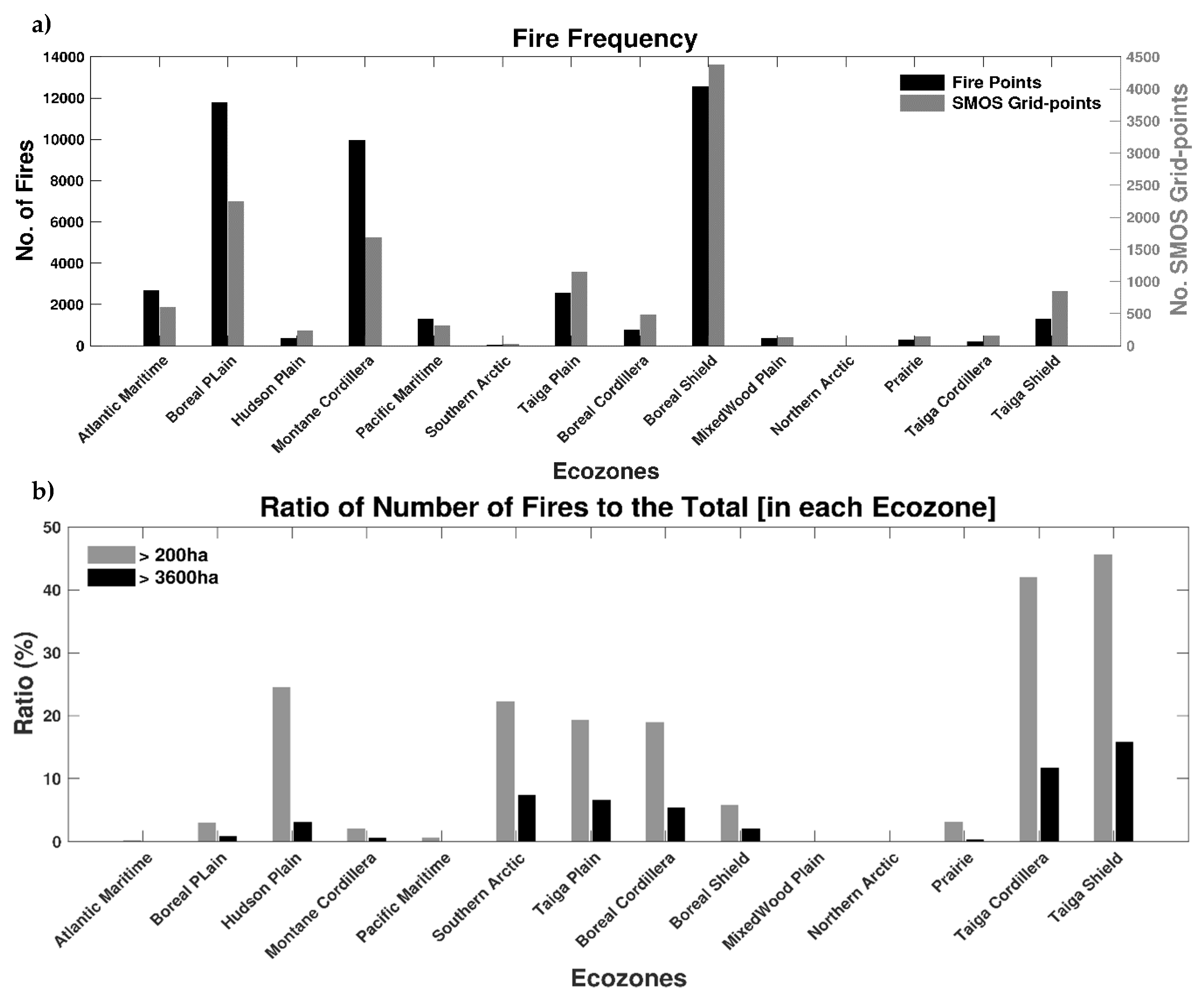
The total number of all fires, as well as the number of SMOS grid cells within each of the ecozones, is illustrated in Figure 2a. Based on Figure 1 and Figure 2a, it is clear that the majority of the fires occurred within the Boreal ecozones (i.e., Boreal plain and Boreal shield) and in the Montane cordillera. In some ecozones, such as the Boreal plain and Montane cordillera, there are few SMOS grid pixels, which implies a relatively large number of fires occurred within each SMOS grid pixel in that ecozone (see Figure 2a). Figure 2b illustrates the ratio of the number of fires exceeding a specific size (200 ha and 3600 ha) to the total number of fires in each ecozone.
3. Results
To illustrate the potential sensitivity of SMOS soil moisture products prior to a fire initiation, in Figure 3, we show some selected soil moisture time series prior to the onset of fire. In Figure 3, we included a SMAP time series for reference only and to potentially highlight the consistency between two passive microwave L-band sensors shown to be sensitive to soil moisture. We did not complete the histogram analysis of the SMAP data set as the time series is relatively short for the SMAP sensor (since 2015). Four randomly selected fires (unique fire identifier is indicated in square brackets on the figure subtitles) of various burned area sizes in four major ecozones were selected. The first fire located in the Boreal Plain Ecozone (Figure 3a), identified as SK-2017-002977 (57.31, −109.56), occurred in the late summer of 2017 and burned approximately 427 ha in area. The Boreal Shield fire (Figure 3b), identified as SK-2016-002542 (57.67, −108.58), took place in the early summer 2016 and burned approximately 24,204.2 ha of forested land. The third fire presented occurred in the Hudson Plain ecozone (Figure 3c) was identified as MB-2015-NE061 (56.37, −93.34) and took place in the early summer 2015 burning approximately 662.6 ha. Finally, the fourth fire identified as BC-2015-C50146 (52.22, −124.13), also known as the “Puntzi Lake fire”, took place in mid-summer 2015, burned approximately 8089 ha, and was located in the Montane Cordillera ecozone (Figure 3d; here, we include a Montane Cordillera fire as the SMOS quality flags associated with topographic impacts on data quality were not present for the specific pixel containing the fire). It is clear from all four cases (Figure 3a–d), that both SMAP and SMOS reveal a drying trend, at least one week prior to fire initiation, which indicates the two satellite systems’ sensitivity to the drying of the surface prior to the onset of a fire. However, it should be noted that both sensors vary in terms of magnitude of the dryness. The sudden “jumps” in soil moisture, particularly in the Hudson Plain (Figure 3c) and in the Montane Cordillera fires (Figure 3d), are due to small local rainfall events and the uncertainty of the products ([45,59]; an unbiased RMSE of approximately ± 0.04 m3m−3). Although illustrative of soil moisture time series prior to fire and potentially for the application of these products for identifying potential wildfire hotspots, Figure 3 is anecdotal. Therefore, we expand our analysis to all 48,754 of the fires recorded in the National Fire Database.
Figure 4 illustrates histograms of the soil moisture anomalies 3-days, 5-days, and 7-days (column-wise, left to right) prior to the occurrence of fire, for Atlantic Maritime, Boreal Plain, Pacific Maritime, Taiga Plain, Boreal Shield, and Taiga Shield (row-wise, top to bottom) ecozones, respectively. These seven ecozones are selected based on relatively large numbers of fires (as shown in Figure 2a). It is clear from Figure 4 that the histogram distributions are quite different in each ecozone, although the shape of the distributions are somewhat consistent at 3-days, 5-days, and 7-days prior to the occurrence of fire. The KS normality test of the distribution indicates that, for all ecozones except the Taiga Shield, at 3-days prior to the fire (Figure 4p), the test statistic (ks) is greater than the critical value (cv) rejecting the null-hypothesis at 5%. In other words, the KS test suggests, that, for all ecozones (except that previously mentioned), the soil-moisture anomalies are not normally distributed (hv = 1). All the KS test statistics are displayed on the top-left of each sub-figure in Figure 4.
For all the ecozones, except the Atlantic Maritime (Figure 4a–c), the histograms indicate a negative shift suggesting drier soil conditions. The skewness (Sk) of the histogram are computed using MATLAB’s skewness function. The skewness (Sk) parameter displayed on the top-right of each histogram indicates that almost all histograms, except the Atlantic Maritime (Figure 4a–c) and Boreal Shield (Figure 4m–o), show a positive skewness, suggesting a left leaning distribution, i.e., negative soil moisture anomaly. In Atlantic Maritime (Figure 4a–c) and Boreal Shield (Figure 4m–o), the histogram indicates a slight positive shift (negative skewness), suggesting relatively wetter conditions prior to fire initiation.
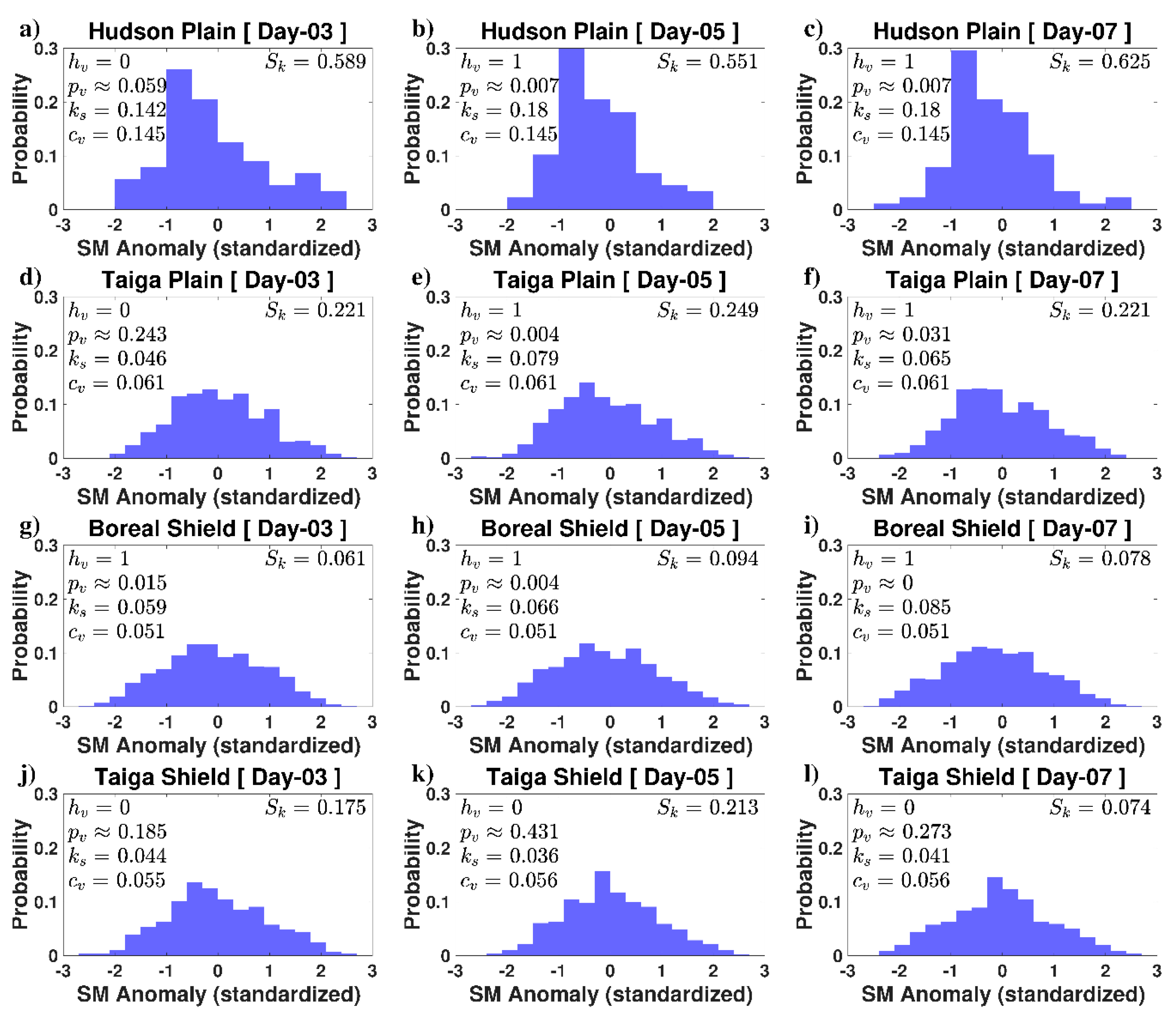
Previous research demonstrates that, although there is a much larger number of small fires, many are subjected to fire suppression measures and thus represent much less area burned than observed in large fires [7,64,65]; therefore, we focused on larger fires (>200 ha) for the subsequent analysis. The contrast between total number of fires vs the number of large fires is evident in Figure 2 and is consistent with previously published studies (see also Figure 4 in Reference [7]). For example, Figure 2a indicates that, although there were approximately 3000 fires that occurred in Atlantic Maritime ecozone during the study period, only a very small fraction were large fires. Similarly, less than 5% of the ~12,000 fires in the Boreal ecozones (Boreal Plain and Boreal Shield) were considered large fires. To examine the importance of SM anomaly on large fires, we recomputed the histogram (Figure 5) after excluding all the fires with burned area < 200 ha. The histogram (Figure 5) shows the normalized SM anomaly at 3-days, 5-days, and 7-days (column-wise, left to right) prior to the occurrence of fire, for the Hudson Plain, Taiga Plain, Boreal Shield, and Taiga Shield ecozones (row-wise, top to bottom). Some ecozones were excluded as the number of large fires (>200 ha) were very small over the time period resulting in insufficient data to form a histogram. Figure 5 demonstrates that for all ecozones except the Taiga shield (Figure 5j–l), the soil moisture anomalies show a shift towards a negative anomaly (dry soil moisture anomaly as also indicated a positive skewness values) observable for 3-days, 5-days, and 7-days (columns left-to-right) prior to the fire initiation. The SMOS observed SM anomaly does not show similar sensitivity over Taiga shield, which may be related to numerous open water surfaces over the area, which will have an influence on the SMOS retrieval accuracy [44].
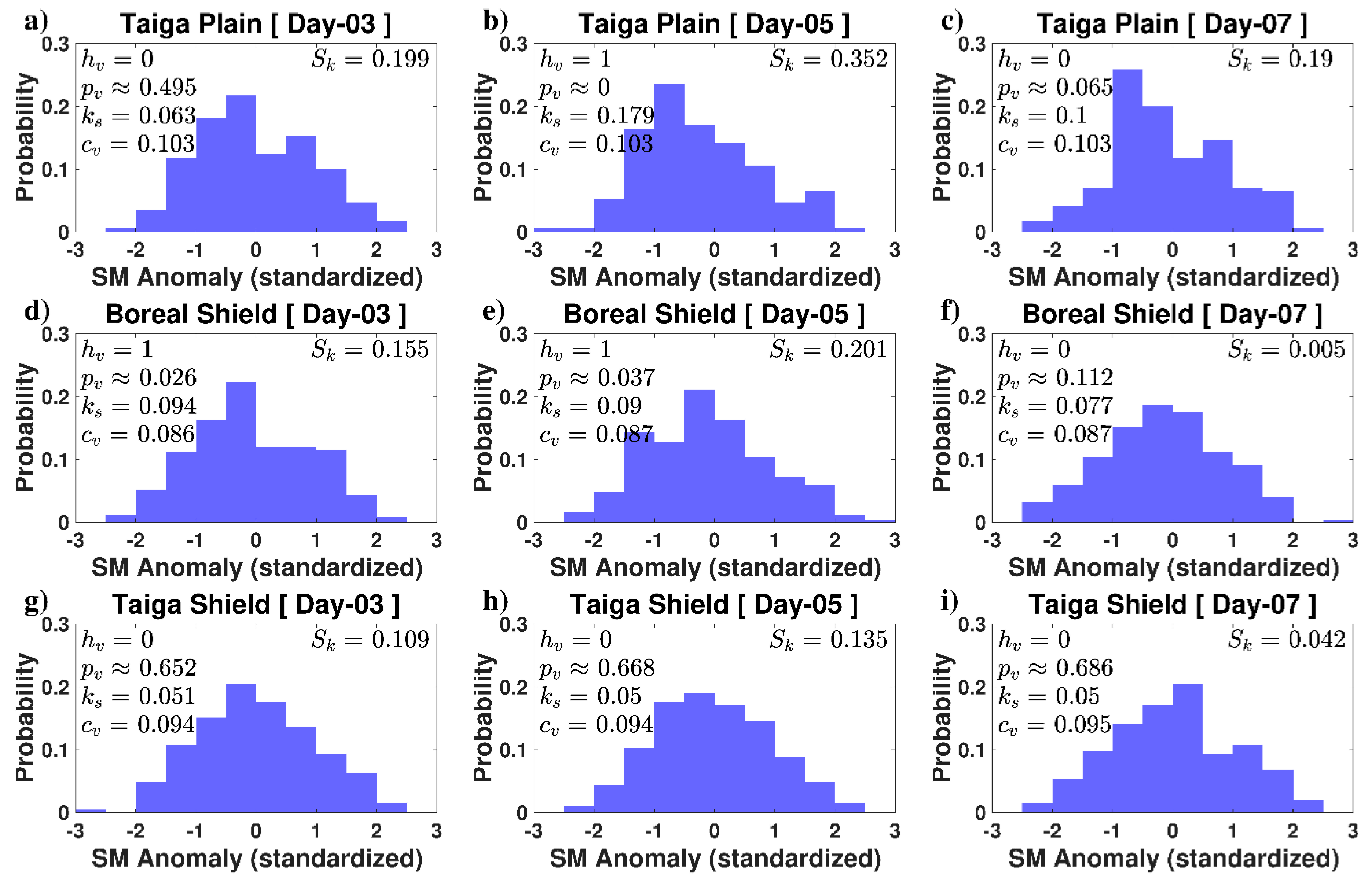
Distributions of fires with burned area greater than 3600 ha are illustrated in Figure 6. Histograms could only be created for three ecozones: the Taiga Plain, the Boreal Shield, and the Taiga Shield. Overall, the figure suggests that SMOS SM anomaly observable 3, 5, and 7 days prior to the fire particularly over the Boreal Shield captures the drying surface conditions prior to the occurrence of fire, as indicated by the shift in the distribution towards negative anomalies. Capturing the SM anomaly over the Boreal Shield ecozone is particularly important since this ecozone is one of the largest and most diverse in-terms of species and has a wide range of climatic and ecosystem conditions [7,13]. The anomaly distributions illustrated in Figure 6d–f and Figure 5g–i suggest the SMOS SM product was sensitive to dry surface conditions in advance of fire in this ecozone.
4. Discussion
The results of this study demonstrated that there is skewness in the SMOS observed soil moisture distributions towards negative anomalies prior to the fire ignition for the majority of ecoregions. By comparing the histograms of respective ecozones in Figure 4 and Figure 5, we can see that Figure 5 shows a relatively greater positive skewness than Figure 4, which implies SMOS SM anomalies are sensitive to the drier surface conditions prior to larger wildfires. Within the regions analyzed, the SMOS product includes quality flags on the retrieval. The quality flags denote potential issues associated with the product. These flags may be related to regions of high topographic variation, denser forest canopies, or rainfall during the retrieval; when these flags are present, it is recommended that the data be interpreted with caution. While the present study does not explicitly separate the influence of various science flags on SMOS SM distributions over the boreal forest, the majority of the regions analyzed included science flags that suggest that the retrieval is impacted by vegetation. Although there are some studies that demonstrate that SMOS has some correlation with ground observations of soil moisture in the boreal forest in Canada, these studies are limited to only one or two pixels (e.g., 50,54). Therefore, it was somewhat of an open question regarding the value of product in this environment for the purposes of identifying surface drying prior to wildfire initiation.
We recognize that there are several limitations to this study overall. As illustrated in our results (Figure 4, Figure 5 and Figure 6), there are a significant number of fires that also initiated under wetter soil moisture anomalies. Soil moisture is among a multitude of factors necessary for wildfire; therefore, further analysis of vegetation conditions, fine fuel abundance, and connectivity would be necessary to further outline the role of satellite observed soil moisture anomalies on individual fires. Furthermore, it is very likely a soil moisture threshold may exist in several regions; below this critical moisture threshold, the likelihood of fire ignition is possible [66]; in many cases, this threshold may not be associated with a negative soil moisture anomaly. This study focused on retrieved SMOS SM products (e.g., SMOS SM Level-2 used in this study), in regions of high vegetation where the product may be impacted by significant vegetation water content. Therefore, using a forward model better adapted to each ecozone in conjunction with a land surface model, which assimilates the satellite brightness temperature (along with site specific parameters and uncertainties), may provide better soil moisture estimates. Finally, the spatial and temporal resolution of data could be improved by using advanced downscaling techniques, which may result in better accuracy pin-pointing the hot-spots when also combined with vegetation density.
5. Conclusions
It is well known that dry land surface conditions precede wildfire and that methods to identify potential wildfire hot-spots in advance are useful for predicting wildfire occurrence. However, it is not known the degree to which satellites sensitive to SM are useful for this purpose, particularly over the various boreal ecozones within Canada. In this study, surface SM conditions preceding wildfire occurrences across various Canadian ecozones were analyzed for the period 2010–2017, using SMOS satellite-derived SM data. Results show that, over the majority of the ecozones, histograms created from SM anomalies at 3, 5, and 7 days prior to the fire show a negative shift suggested that the satellite-based SM products were sensitive to surface drying prior to the occurrence of the wildfire. We would recommend further evaluation of these products over Canada, particularly if they are integrated into operational models.
Author Contributions
Conceptualization & methodology, J.T.A., A.A.B., Z.G. formal analysis, J.T.A., A.A.B.; data curation, writing—original draft preparation, J.T.A., M.O., A.A.B.; writing—review and editing, J.T.A., A.A.B., Z.G., M.O.; visualization, J.T.A., M.O.; funding acquisition, A.A.B. All authors have read and agreed to the published version of the manuscript.
Funding
This work was supported by the Canadian Space Agency (CSA) and the Natural Sciences and Engineering Research Council of Canada and the Canada First Research Excellence Fund.
Acknowledgments
The authors would like to thank Adam Bonnycastle, GIS specialist, Department of Geography, Environment and Geomatics, University of Guelph, for his assistance with the ArcGIS software.
Conflicts of Interest
The authors declare no conflict of interest. The funders had no role in the design of the study; in the collection, analyses, or interpretation of data; in the writing of the manuscript, or in the decision to publish the results.
References
- Krikken, F.; Lehner, F.; Drobyshev, I.; van Oldenborgh, G.J. Attribution of the role of global warming in the forest fires in Sweden 2018. In Geophysical Research Abstracts, Proceedings of the EGU General Assembly, Vienna, Austria, 7–12 April 2019; EGU2019-17342; EGU: Munich, Germany, 2019; Volume 21. [Google Scholar]
- Turco, M.; Rosa-Cánovas, J.J.; Bedia, J.; Jerez, S.; Montávez, J.P.; Llasat, M.-C.; Provenzale, A. Exacerbated fires in Mediterranean Europe due to anthropogenic warming projected with non-stationary climate-fire models. Nat. Commun. 2018, 9, 3821. [Google Scholar] [CrossRef]
- Gillett, N.P.; Weaver, A.J.; Zwiers, F.W.; Flannigan, M. Detecting the effect of climate change on Canadian forest fires. Geophys. Res. Lett. 2004, 31. [Google Scholar] [CrossRef] [Green Version]
- Flannigan, M.; Bergeron, Y.; Engelmark, O.; Wotton, B. Future wildfire in circumboreal forests in relation to global warming. J. Veg. Sci. 1998, 9, 469–476. [Google Scholar] [CrossRef]
- Keeley, J.; Syphard, A. Climate Change and Future Fire Regimes: Examples from California. Geoscience 2016, 6, 37. [Google Scholar] [CrossRef] [Green Version]
- Bolton, D.K.; Coops, N.C.; Wulder, M.A. Characterizing residual structure and forest recovery following high-severity fire in the western boreal of Canada using Landsat time-series and airborne lidar data. Remote. Sens. Environ. 2015, 163, 48–60. [Google Scholar] [CrossRef]
- Stocks, B.J.; Mason, J.A.; Todd, J.B.; Bosch, E.M.; Wotton, B.M.; Amiro, B.D.; Flannigan, M.D.; Hirsch, K.G.; Logan, K.A.; Martell, D.L.; et al. Large forest fires in Canada, 1959–1997. J. Geophys. Res. Atmos. 2002, 107, FFR-5. [Google Scholar] [CrossRef]
- Amiro, B.D.; Todd, J.B.; Wotton, B.M.; Logan, K.A.; Flannigan, M.D.; Stocks, B.J.; Mason, J.A.; Martell, D.L.; Hirsch, K.G. Direct carbon emissions from Canadian forest fires, 1959–1999. Can. J. For. Res. 2001, 31, 512–525. [Google Scholar] [CrossRef]
- Amiro, B.; Cantin, A.; Flannigan, M.; De Groot, W. Future emissions from Canadian boreal forest fires. Can. J. For. Res. 2009, 39, 383–395. [Google Scholar] [CrossRef]
- Alexander, M.E. Calculating and interpreting forest fire intensities. Can. J. Bot. 1982, 60, 349–357. [Google Scholar] [CrossRef]
- Flannigan, M.; Stocks, B.; Turetsky, M.; Wotton, M.; Flannigan, M. Impacts of climate change on fire activity and fire management in the circumboreal forest. Glob. Chang. Boil. 2009, 15, 549–560. [Google Scholar] [CrossRef]
- Wotton, B.M.; Nock, C.A.; Flannigan, M. Forest fire occurrence and climate change in Canada. Int. J. Wildland Fire 2010, 19, 253–271. [Google Scholar] [CrossRef]
- Stinson, G.; Kurz, W.A.; Smyth, C.E.; Neilson, E.T.; Dymond, C.C.; Metsaranta, J.M.; Boisvenue, C.; Rampley, G.J.; Li, Q.; White, T.M.; et al. An inventory-based analysis of Canada’s managed forest carbon dynamics, 1990 to 2008. Glob. Chang. Biol. 2011, 17, 2227–2244. [Google Scholar] [CrossRef] [Green Version]
- Chowdhury, E.H.; Hassan, Q.K. Development of a New Daily-Scale Forest Fire Danger Forecasting System Using Remote Sensing Data. Remote. Sens. 2015, 7, 2431–2448. [Google Scholar] [CrossRef] [Green Version]
- LeBlon, B. Monitoring Forest Fire Danger with Remote Sensing. Nat. Hazards 2005, 35, 343–359. [Google Scholar] [CrossRef]
- Lin, H.; Liu, Z.; Zhao, T.; Zhang, Y. Early Warning System of Forest Fire Detection Based on Video Technology. In Proceedings of the Lecture Notes in Electrical Engineering; Liu, X.Z., Ye, Y.Y., Eds.; Springer: Heidelberg/Berlin, Germany, 2013; Volume 272, pp. 751–758. [Google Scholar]
- Leckie, D.G. Advances in remote sensing technologies for forest surveys and management. Can. J. For. Res. 1990, 20, 464–483. [Google Scholar] [CrossRef]
- Chisholm, R.A.; Cui, J.; Lum, S.K.Y.; Chen, B.M. UAV LiDAR for below-canopy forest surveys. J. Unmanned Veh. Syst. 2013, 1, 61–68. [Google Scholar] [CrossRef] [Green Version]
- Den Breejen, E.; Breuers, M.; Cremer, F.; Kemp, R.; Roos, M.; Schutte, K.; De Vries, J.S. Autonomous forest fire detection. In Proceedings of the 3rd International Conference on Forest Fire Research, Luso, Portugal, 16–20 November 1998; pp. 2003–2012. [Google Scholar]
- Deeming, J.E.; Burgan, R.E.; Cohen, J.D. The National Fire-Danger Rating System—1978; Gen. Tech. Rep. INT-39; U.S. Department of Agriculture, Forest Service, Intermountain Forest and Range Experiment Station: Ogden, UT, USA, 1977; 63p.
- Chaparro, D.; Vall-llossera, M.; Piles, M. Chapter 11: A Review on European Remote Sensing Activities in Wildland Fires Prevention. In Remote Sensing of Hydrometeorological Hazards; CRC Press: Boca Raton, FL, USA, 2017; p. 237. [Google Scholar]
- Canadian Forest Service. Development and Structure of the Canadian Forest Fire Behaviour Prediction System; Information Report ST-X-3; Canadian Forest Service: Ottawa, ON, Canadian, 1992; 63p.
- Leblon, B.; Bourgeau-Chavez, L.; San-Miguel-Ayanz, J. Use of remote sensing in wildfire management (Chapter 3). In Sustainable Development—Authoritative and Leading Edge Content for Environmental Management; INTECH: Croatia, Rijeka, 2012; pp. 55–82. [Google Scholar]
- Dacamara, C.C.; Calado, T.J.; Ermida, S.L.; Trigo, I.F.; Amraoui, M.; Turkman, K.F. Calibration of the Fire Weather Index over Mediterranean Europe based on fire activity retrieved from MSG satellite imagery. Int. J. Wildland Fire 2014, 23, 945. [Google Scholar] [CrossRef]
- Hains, D.A.; Johnson, V.J.; Main, W.A. An Assessment of Three Measures of Long-Term Moisture Deficiency before Critical Fire Periods; Research Paper NC-131; North Central Forest Experiment Station, United States Department of Agriculture (USDA) Forest Service: St. Paul, MN, USA, 1976.
- Koster, R.; Suarez, M.J. Soil Moisture Memory in Climate Models. J. Hydrometeorol. 2001, 2, 558–570. [Google Scholar] [CrossRef]
- Seneviratne, S.I.; Koster, R.; Guo, Z.; Dirmeyer, P.A.; Kowalczyk, E.; Lawrence, D.; Liu, P.; Mocko, D.; Lu, C.-H.; Oleson, K.W.; et al. Soil Moisture Memory in AGCM Simulations: Analysis of Global Land–Atmosphere Coupling Experiment (GLACE) Data. J. Hydrometeorol. 2006, 7, 1090–1112. [Google Scholar] [CrossRef] [Green Version]
- Ambadan, J.T.; Berg, A.A.; Merryfield, W.J.; Lee, W.-S. Influence of snowmelt on soil moisture and on near surface air temperature during winter–spring transition season. Clim. Dyn. 2017, 51, 1295–1309. [Google Scholar] [CrossRef]
- Medler, M.J.; Montesano, P.; Robinson, D. Examining the Relationship between Snowfall and Wildfire Patterns in the Western United States. Phys. Geogr. 2002, 23, 335–342. [Google Scholar] [CrossRef]
- Westerling, A.L.; Hidalgo, H.G.; Cayan, D.R.; Swetnam, T.W. Warming and Earlier Spring Increase Western U.S. Forest Wildfire Activity. Science 2006, 313, 940–943. [Google Scholar] [CrossRef] [Green Version]
- Jia, S.; Kim, S.H.; Nghiem, S.; Kafatos, M.C. Estimating Live Fuel Moisture Using SMAP L-Band Radiometer Soil Moisture for Southern California, USA. Remote. Sens. 2019, 11, 1575. [Google Scholar] [CrossRef] [Green Version]
- Wang, L.; Quan, X.; He, B.; Yebra, M.; Xing, M.; Liu, X. Assessment of the Dual Polarimetric Sentinel-1A Data for Forest Fuel Moisture Content Estimation. Remote. Sens. 2019, 11, 1568. [Google Scholar] [CrossRef] [Green Version]
- Konings, A.G.; Piles, M.; Rötzer, K.; McColl, K.A.; Chan, S.K.; Entekhabi, D. Vegetation optical depth and scattering albedo retrieval using time series of dual-polarized L-band radiometer observations. Remote. Sens. Environ. 2016, 172, 178–189. [Google Scholar] [CrossRef]
- Konings, A.G.; Piles, M.; Das, N.; Entekhabi, D. L-band vegetation optical depth and effective scattering albedo estimation from SMAP. Remote. Sens. Environ. 2017, 198, 460–470. [Google Scholar] [CrossRef]
- Piles, M.; Sanchez, N.; Vall-Llossera, M.; Camps, A.; Martínez-Fernández, J.; Martinez, J.; Gonzalez-Gambau, V. A Downscaling Approach for SMOS Land Observations: Evaluation of High-Resolution Soil Moisture Maps over the Iberian Peninsula. IEEE J. Sel. Top. Appl. Earth Obs. Remote. Sens. 2014, 7, 3845–3857. [Google Scholar] [CrossRef] [Green Version]
- Naeimi, V.; Scipal, K.; Bartalis, Z.; Hasenauer, S.; Wagner, W. An Improved Soil Moisture Retrieval Algorithm for ERS and METOP Scatterometer Observations. IEEE Trans. Geosci. Remote. Sens. 2009, 47, 1999–2013. [Google Scholar] [CrossRef]
- Entekhabi, D.; Njoku, E.G.; O’Neill, P.E.; Kellogg, K.H.; Crow, W.T.; Edelstein, W.N.; Entin, J.K.; Goodman, S.D.; Jackson, T.J.; Johnson, J.; et al. The Soil Moisture Active Passive (SMAP) Mission. Proc. IEEE 2010, 98, 704–716. [Google Scholar] [CrossRef]
- Scaini, A.; Sanchez, N.; Vicente-Serrano, S.; Martínez-Fernández, J. SMOS-derived soil moisture anomalies and drought indices: A comparative analysis usingin situmeasurements. Hydrol. Process. 2014, 29, 373–383. [Google Scholar] [CrossRef]
- Martínez-Fernández, J.; González-Zamora, Á.; Sanchez, N.; Gumuzzio, A. A soil water based index as a suitable agricultural drought indicator. J. Hydrol. 2015, 522, 265–273. [Google Scholar] [CrossRef]
- Martínez-Fernández, J.; González-Zamora, Á.; Sánchez, N.; Gumuzzio, A.; Herrero-Jiménez, C. Satellite soil moisture for agricultural drought monitoring: Assessment of the SMOS derived Soil Water Deficit Index. Remote. Sens. Environ. 2016, 177, 277–286. [Google Scholar] [CrossRef]
- Sanchez, N.; González-Zamora, Á.; Piles, M.; Martínez-Fernández, J. A New Soil Moisture Agricultural Drought Index (SMADI) Integrating MODIS and SMOS Products: A Case of Study over the Iberian Peninsula. Remote. Sens. 2016, 8, 287. [Google Scholar] [CrossRef] [Green Version]
- Ross, M.A.; Ponce-Campos, G.E.; Barnes, M.L.; Hottenstein, J.D.; Moran, M.S. Response of grassland ecosystems to prolonged soil moisture deficit. In Proceedings of the EGU General Assembly Conference Abstracts, Vienna, Austria, 27 April–2 May 2014. [Google Scholar]
- White, J.; Berg, A.A.; Champagne, C.; Warland, J.; Zhang, Y. Canola yield sensitivity to climate indicators and passive microwave-derived soil moisture estimates in Saskatchewan, Canada. Agric. For. Meteorol. 2019, 268, 354–362. [Google Scholar] [CrossRef]
- Kerr, Y.H.; Richaume, P.; Wigneron, J.-P.; Gruhier, C.; Juglea, S.E.; Leroux, D.; Delwart, S.; Waldteufel, P.; Ferrazzoli, P.; Mahmoodi, A.; et al. The SMOS Soil Moisture Retrieval Algorithm. IEEE Trans. Geosci. Remote. Sens. 2012, 50, 1384–1403. [Google Scholar] [CrossRef]
- Kerr, Y.; Al-Yaari, A.; Rodríguez-Fernández, N.; Parrens, M.; Molero, B.; Leroux, D.; Bircher, S.; Mahmoodi, A.; Mialon, A.; Richaume, P.; et al. Overview of SMOS performance in terms of global soil moisture monitoring after six years in operation. Remote. Sens. Environ. 2016, 180, 40–63. [Google Scholar] [CrossRef]
- Forkel, M.; Thonicke, K.; Beer, C.; Cramer, W.; Bartalev, S.; Schmullius, C. Extreme fire events are related to previous-year surface moisture conditions in permafrost-underlain larch forests of Siberia. Environ. Res. Lett. 2012, 7, 044021. [Google Scholar] [CrossRef]
- Shvetsov, E. Fire Danger Estimation in Siberia Using SMOS Data. EGU General Assembly Conference Abstracts (Vol. 15). April 2013. Available online: http://neespi.org/web-content/meetings/EGU_2013/Shvetsov.pdf (accessed on 8 May 2020).
- Chaparro, D.; Vayreda, J.; Martínez-Vilalta, J.; Vall-Llossera, M.; Banque, M.; Camps, A.; Piles, M. SMOS and climate data applicability for analyzing forest decline and forest fires. In Proceedings of the 2014 IEEE Geoscience and Remote Sensing Symposium, Quebec City, QC, Canada, 13–18 July 2014; pp. 1069–1072. [Google Scholar] [CrossRef]
- Chaparro, D.; Piles, M.; Vall-Llossera, M. Remotely Sensed Soil Moisture as a Key Variable in Wildfires Prevention Services. In Satellite Soil Moisture Retrieval; Elsevier: Amsterdam, The Netherlands, 2016; pp. 249–269. [Google Scholar]
- Gherboudj, I.; Magagi, R.; Goita, K.; Berg, A.A.; Toth, B.; Walker, A. Validation of SMOS Data over Agricultural and Boreal Forest Areas in Canada. IEEE Trans. Geosci. Remote. Sens. 2012, 50, 1623–1635. [Google Scholar] [CrossRef]
- Magagi, R.; Berg, A.A.; Goita, K.; Belair, S.; Jackson, T.J.; Toth, B.; Walker, A.; McNairn, H.; O’Neill, P.E.; Moghaddam, M.; et al. Canadian Experiment for Soil Moisture in 2010 (CanEx-SM10): Overview and Preliminary Results. IEEE Trans. Geosci. Remote. Sens. 2012, 51, 347–363. [Google Scholar] [CrossRef] [Green Version]
- Adams, J.R.; McNairn, H.; Berg, A.A.; Champagne, C. Evaluation of near-surface soil moisture data from an AAFC monitoring network in Manitoba, Canada: Implications for L-band satellite validation. J. Hydrol. 2015, 521, 582–592. [Google Scholar] [CrossRef]
- McNairn, H.; Jackson, T.J.; Wiseman, G.; Bélair, S.; Berg, A.A.; Bullock, P.; Colliander, A.; Cosh, M.H.; Kim, S.; Magagi, R.; et al. The Soil Moisture Active Passive Validation Experiment 2012 (SMAPVEX12): Prelaunch Calibration and Validation of the SMAP Soil Moisture Algorithms. IEEE Trans. Geosci. Remote. Sens. 2014, 53, 2784–2801. [Google Scholar] [CrossRef]
- Djamai, N.; Magagi, R.; Goïta, K.; Hosseini, M.; Cosh, M.H.; Berg, A.A.; Toth, B. Evaluation of SMOS soil moisture products over the CanEx-SM10 area. J. Hydrol. 2015, 520, 254–267. [Google Scholar] [CrossRef]
- Champagne, C.; Rowlandson, T.; Berg, A.A.; Burns, T.; L’Heureux, J.; Tetlock, E.; Adams, J.R.; McNairn, H.; Toth, B.; Itenfisu, D. Satellite surface soil moisture from SMOS and Aquarius: Assessment for applications in agricultural landscapes. Int. J. Appl. Earth Obs. Geoinformation 2016, 45, 143–154. [Google Scholar] [CrossRef] [Green Version]
- Canadian Forest Service. National Fire Database–Agency Fire Data; Natural Resources Canada, Canadian Forest Service, Northern Forestry Centre: Edmonton, AB, Canada, 2018. Available online: http://cwfis.cfs.nrcan.gc.ca/ha/nfdb (accessed on 20 February 2020).
- Parisien, M.-A.; Peters, V.S.; Wang, Y.; Little, J.M.; Bosch, E.M.; Stocks, B.J. Spatial patterns of forest fires in Canada, 1980–1999. Int. J. Wildland Fire 2006, 15, 361–374. [Google Scholar] [CrossRef]
- Kerr, Y.H.; Waldteufel, P.; Wigneron, J.-P.; Delwart, S.; Cabot, F.; Boutin, J.; Escorihuela, M.J.; Font, J.; Reul, N.; Gruhier, C.; et al. The SMOS Mission: New Tool for Monitoring Key Elements ofthe Global Water Cycle. Proc. IEEE 2010, 98, 666–687. [Google Scholar] [CrossRef] [Green Version]
- Chan, S.K.; Bindlish, R.; O’Neill, P.E.; Njoku, E.; Jackson, T.; Colliander, A.; Chen, F.; Burgin, M.; Dunbar, S.; Piepmeier, J.; et al. Assessment of the SMAP Passive Soil Moisture Product. IEEE Trans. Geosci. Remote. Sens. 2016, 54, 4994–5007. [Google Scholar] [CrossRef]
- Chan, S.; Bindlish, R.; O’Neill, P.E.; Jackson, T.; Njoku, E.; Dunbar, S.; Chaubell, J.; Piepmeier, J.; Yueh, S.; Entekhabi, D.; et al. Development and assessment of the SMAP enhanced passive soil moisture product. Remote. Sens. Environ. 2018, 204, 931–941. [Google Scholar] [CrossRef] [Green Version]
- Pellarin, T.; Mialon, A.; Biron, R.; Coulaud, C.; Gibon, F.; Kerr, Y.; Lafaysse, M.; Mercier, B.; Morin, S.; Redor, I.; et al. Three years of L-band brightness temperature measurements in a mountainous area: Topography, vegetation and snowmelt issues. Remote. Sens. Environ. 2016, 180, 85–98. [Google Scholar] [CrossRef]
- Mialon, A.; Coret, L.; Kerr, Y.; Secherre, F.; Wigneron, J.-P. Flagging the Topographic Impact on the SMOS Signal. IEEE Trans. Geosci. Remote. Sens. 2008, 46, 689–694. [Google Scholar] [CrossRef]
- Marshall, I.B.; Schut, P.H.; Ballard, M. A National Ecological Framework for Canada: Attribute Data; Agriculture and Agri-Food Canada, Research Branch, Centre for Land and Biological Resources Research and Environment Canada, State of the Environment Directorate, Ecozone Analysis Branch: Ottawa, ON, Canada; Hull, QC, Canada, 1999. Available online: http://sis.agr.gc.ca/cansis/nsdb/ecostrat/1999report/index.html (accessed on 20 February 2020).
- Hanes, C.C.; Wang, X.; Jain, P.; Parisien, M.-A.; Little, J.M.; Flannigan, M.D. Fire-regime changes in Canada over the last half century. Can. J. For. Res. 2019, 49, 256–269. [Google Scholar] [CrossRef]
- Girardin, M.P.; Mudelsee, M. Past and future changes in Canadian boreal wildfire activity. Ecol. Appl. 2008, 18, 391–406. [Google Scholar] [CrossRef] [PubMed]
- Gedalof, Z. Climate and Spatial Patterns of Wildfire in North America. In The Landscape Ecology of Fire; McKenzie, D., Miller, C., Falk, D., Eds.; Springer: Dordrecht, The Netherlands, 2011; pp. 89–116. [Google Scholar]
Figure 1.
Spatial distribution of all fires over a 8-year period (2010–2017), over various ecozones in Canada. The red dots indicate the fire locations. The main ecozones considered are the Boreal Shield, Boreal Plain, Atlantic Maritime, Pacific Maritime, Taiga Plain, and the Taiga Shield.
Figure 1.
Spatial distribution of all fires over a 8-year period (2010–2017), over various ecozones in Canada. The red dots indicate the fire locations. The main ecozones considered are the Boreal Shield, Boreal Plain, Atlantic Maritime, Pacific Maritime, Taiga Plain, and the Taiga Shield.

Figure 2.
Frequency of all fires and the number of SMOS (Soil Moisture and Ocean Salinity) grid cells that are representative of the fires (a); ratio of the number of fires to the total (b).
Figure 2.
Frequency of all fires and the number of SMOS (Soil Moisture and Ocean Salinity) grid cells that are representative of the fires (a); ratio of the number of fires to the total (b).

Figure 3.
SMOS (Soil Moisture and Ocean Salinity) and SMAP (Soil Moisture Active Passive) soil moisture time series over two weeks period prior to the onset of fire, for four randomly selected fires in, Boreal Plain (a), Boreal Shield (b), Hudson Plain (c), and Mountane Cordillera (d). The unique fire identifier is indicated in square brackets on the figure subtitles. r is the correlation between SMOS and SMAP soil moisture.

Figure 4.
Histograms of the normalized soil moisture anomaly distribution at 3-days, 5-days, and 7-days (column-wise, left to right) prior to the occurrence of fire, for ecozones Atlantic Maritime (a–c), Boreal Plain (d–f), Pacific Maritime (g–i), Taiga Plain (j–l), Boreal Shield (m–o), and Taiga Shield (p–r), respectively. The parameters h, p, ks, and cv are MATLAB Kolmogorov-Smirnov (KS) test result parameters: ‘h’ is a logical value (0 or 1) indicating the hypothesis test result, i.e., h = 1 indicates rejection of the null hypothesis at the 5% significance level, and h = 0 indicates a failure to reject the null hypothesis. The parameter ‘p’ is the p-value of the test, ks is the test statistic and cv is the critical value of the test. If the test statistic (ks) is greater than the critical value (cv), then the KS test rejects the null-hypothesis. The parameter Sk (top right) indicates the skewness of the distribution. A positive skewness suggests a left leaning distribution, and vice versa. SM = soil moisture.

Figure 5.
Distributions of fires with burned area greater than 200 ha. Soil moisture anomaly distributions at 3-days, 5-days, and 7-days (column-wise, left to right) prior to the occurrence of fire for ecozones Hudson Plain (a–c), Taiga Plain (d–f), Boreal Shield (g–i), and Taiga Shield (j–l), respectively. The parameters h, p, ks, and cv are MATLAB Kolmogorov-Smirnov (KS) test result parameters, as in Figure 4. The parameter Sk (top right) indicates the skewness of the distribution.

Figure 6.
Distributions of fires with burned area greater than 3600 ha, for Taiga Plain (a–c), Boreal Shield (d–f), and Taiga Shield (g–i) ecozones. The parameters h, p, ks, and cv are MATLAB Kolmogorov-Smirnov (KS) test result parameters, as in Figure 4. The parameter Sk (top right) indicates the “skewness” of the distribution.

© 2020 by the authors. Licensee MDPI, Basel, Switzerland. This article is an open access article distributed under the terms and conditions of the Creative Commons Attribution (CC BY) license (http://creativecommons.org/licenses/by/4.0/).
Share and Cite
MDPI and ACS Style
Thomas Ambadan, J.; Oja, M.; Gedalof, Z.; Berg, A.A. Satellite-Observed Soil Moisture as an Indicator of Wildfire Risk. Remote Sens. 2020, 12, 1543. https://doi.org/10.3390/rs12101543
AMA Style
Thomas Ambadan J, Oja M, Gedalof Z, Berg AA. Satellite-Observed Soil Moisture as an Indicator of Wildfire Risk. Remote Sensing. 2020; 12(10):1543. https://doi.org/10.3390/rs12101543
Chicago/Turabian StyleThomas Ambadan, Jaison, Matilda Oja, Ze’ev Gedalof, and Aaron A. Berg. 2020. "Satellite-Observed Soil Moisture as an Indicator of Wildfire Risk" Remote Sensing 12, no. 10: 1543. https://doi.org/10.3390/rs12101543
Note that from the first issue of 2016, this journal uses article numbers instead of page numbers. See further details here.