Democratic Republic of the Congo Tropical Forest Canopy Height and Aboveground Biomass Estimation with Landsat-8 Operational Land Imager (OLI) and Airborne LiDAR Data: The Effect of Seasonal Landsat Image Selection

Abstract

Inventories of tropical forest aboveground biomass (AGB) are often imprecise and sparse. Increasingly, airborne Light Detection And Ranging (LiDAR) and satellite optical wavelength sensor data are used to map tree height and to estimate AGB. In the tropics, cloud cover is particularly prevalent and so several years of satellite observations must be considered. This may reduce mapping accuracy because of seasonal and inter-annual changes in the forest reflectance. In this paper, the sensitivity of airborne LiDAR and Landsat-8 Operational Land Imager (OLI) based dominant canopy height and AGB 30 m mapping is assessed with respect to the season of Landsat acquisition for a ~10,000 Km² tropical forest area in the Democratic Republic of the Congo. A random forest regression estimator is used to predict and assess the 30 m dominant canopy height using LiDAR derived test and training data. The AGB is mapped using an allometric model parameterized with the dominant canopy height and is assessed by comparison with field based 30 m AGB estimates. Experiments are undertaken independently using (i) only a wet season Landsat-8 image, (ii) only a dry season Landsat-8 image, and (iii) both Landsat-8 images. At the study area level there is little reported sensitivity to the season of Landsat image used. The mean dominant canopy height and AGB values are similar between seasons, within 0.19 m and 5 Mg ha⁻¹, respectively. The mapping results are improved when both Landsat-8 images are used with Root Mean Square Error (RMSE) values that correspond to 18.8% of the mean study area mapped tree height (20.4 m) and to 41% of the mean study area mapped AGB (204 Mg ha⁻¹). The mean study area mapped AGB is similar to that reported in other Congo Basin forest studies. The results of this detailed study are illustrated and the implications for tropical forest tree height and AGB mapping are discussed.

1. Introduction

Tropical forests play a key role in the terrestrial carbon cycle with globally significant amounts of carbon stored as aboveground biomass (AGB) [1,2,3]. National inventories of forest AGB are incomplete and imprecise in many tropical countries for several reasons and primarily because tropical forests have highly variable structure and composition that make them difficult to survey [4,5,6]. Forest AGB can be measured using destructive methods, i.e., by cutting and weighing trees which is time consuming and expensive, and so more conventionally is estimated using allometric methods that typically parametrize AGB as a function of tree diameter at breast height, or tree height, and species wood density information [7]. Reliable application of allometric models depends on reliable measurement of these tree biometric parameters [8,9,10].

Remotely sensed data have been used to estimate tropical forest tree height and AGB. Early work used statistical approaches applied to optical wavelength passive satellite data and using allometric models [11,12]. Airborne and terrestrial Light Detection and Ranging (LiDAR) remote sensing provides new capabilities for estimating tree canopy structure and has the potential to improve or even replace allometric models [13,14]. Regional to national scale tree height maps have been derived using either spaceborne or airborne LiDAR data at select locations to derive tree height training data that are used to train classifiers applied to optical wavelength satellite data, typically sensed by Landsat, with AGB derived by applying allometric models to the mapped tree heights [15,16,17].

In many regions cloud is prevalent at the time of overpass of Landsat, especially in the tropics [18,19,20], and the Democratic Republic of Congo (DRC) in western Central Africa is one of the cloudiest tropical regions [21]. Different strategies have been used to handle this cloud issue. For example, Staben et al. [22] mapped tree heights in the Northern territory, Australia, using single date cloud-free 30 m Landsat-5 TM or Landsat-7 ETM+ images and airborne LiDAR tree height training data. Other researchers have extracted multi-temporal metrics from Landsat time series. For example, Xu et al. [16] mapped tree height and AGB across the DRC using the medians (i.e., 50th percentiles) of the red, near infrared (NIR), and the two shortwave Landsat-8 Operational Land Imager (OLI) reflective wavelength bands acquired over three years, with airborne LiDAR tree height training data. Thus, the predictor variables at adjacent pixel locations may have been selected from different years and seasons. Hansen et al. [15] mapped tree heights in Sub-Saharan Africa using 30 m multi-temporal metrics extracted from two years of Landsat-7 ETM+ and Landsat-8 OLI reflectance with tree height training data derived from Geoscience Laser Altimeter System (GLAS) data. However, it is unknown how many cloud free-observations were used, the Landsat 7 ETM+ had about 22% fewer observations due to the scan line corrector issue, and Hansen et al. [15] did not examine the effect of the Landsat acquisition seasonality on the mapping accuracy.

Using longer time periods of Landsat data to extract temporal metrics or to select cloud-free images will increase the possibility of obtaining cloud-free observations. However, this may reduce the capability to reliably map tree height and AGB because of seasonal changes in the forest reflectance associated with wet and dry seasons and because of inter-annual variations, for example, due to drought, and other factors that are subject to ongoing research [23,24,25,26].

In this paper the sensitivity of DRC tree height and AGB estimation with respect to the season of Landsat acquisition is examined for the first time. The study area, composed of approximately 10,000 km² of tropical forest in the western part of the DRC, is dominated by dense tropical evergreen rainforest and is often cloudy with distinct wet and dry seasons. Four airborne discrete return LiDAR 10 km × 2 km transects flown in 2014 were used to derive dominant canopy height training and test data. A single dry and a single wet season Landsat-8 Operational Land Imager (OLI) image acquired over the study area were considered. This was because they were the only images acquired in a two-year period around the LiDAR flight dates that had low (<20%) cloud cover and that were cloud-free over the locations of the airborne LiDAR transects.

The following experiments were undertaken independently three times to map and assess the study area 30 m dominant canopy height and AGB using (i) only the wet season Landsat-8 image, (ii) only the dry season Landsat-8 image, and (iii) both images. A random forest regression estimator was trained using 50% (n = 2639) of the LiDAR 30 m heights and using 30 m Landsat-8 predictor variables defined by the green, red, NIR, and shortwave reflective wavelength bands and spectral band ratios. The dominant canopy height prediction accuracy was evaluated using the remaining 50% of the LiDAR 30 m heights not used to train the model. The random forest regression estimator was used to map the dominant canopy height at 30 m for all the study area and then the corresponding 30 m AGB was mapped by application of recent allometric equations [16]. Field measurements were used to validate the AGB at the equivalent of 43 30 m Landsat pixel locations.

The paper is structured as follows. First, the study area and the data used are described (Section 2), followed by the processes used to map and assess the dominant canopy height and AGB results (Section 3), and then the results (Section 4). The sensitivity of the dominant canopy height and AGB results with respect to the season of the Landsat acquisition and implications of the research are discussed (Section 5) followed by the conclusion (Section 6).

2. Study Area and Data

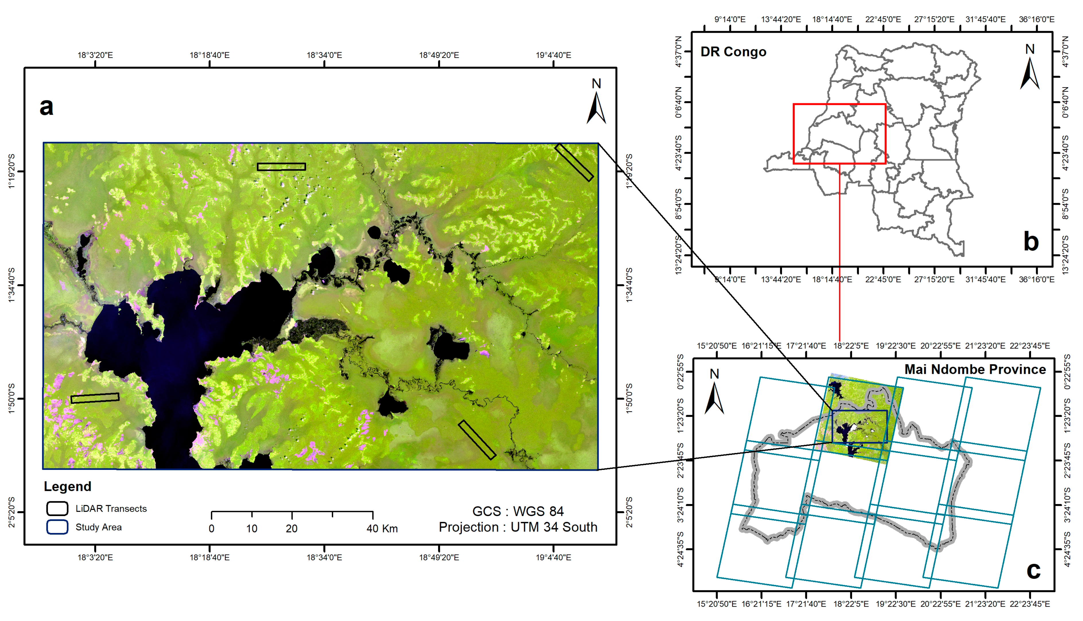
2.1. Study Area

The study area covers 137 km × 80 km of Mai Ndombe province in the DRC (Figure 1). It was selected because it contains airborne LiDAR data and field plot data that can be used to derive AGB. In addition, it is located within a single Landsat Path (180) and Row (061) which reduces Landsat data processing complexity as overlapping images sensed from adjacent Landsat orbits [27] do not need to be processed. The study area falls in the tropical monsoon climate zone and because it lies close to the Equator has two wet and two dry seasons [28]. The Inongo weather station, operated by the Congolese national society of meteorology, is situated near the center of the study area. The annual mean temperature is 24 °C [29] and the annual total rainfall is 1800 mm that falls typically over about 115 days [30]. The main wet season is from September to December. The principal dry season extends from June to August, with a secondary dry season from January to February.

The majority of the study area is covered by dense tropical evergreen rainforest with low lying parts that can be flooded in the wet seasons and includes the northern end of Lake Mai Ndombe [19,31]. People subsist on the terra firme non-forest rural complex (evident in Figure 1a in pink tones), primarily growing cassava, corn, sorghum, upland rice, and peanuts and practicing slash and burn agriculture [32,33]. The main forest characteristics are high tree crown cover (70–100%) with mature tree heights of 35–45 m and predominantly evergreen heterogeneous shade tolerant species [30,31]. The interior forest is relatively undisturbed but at risk of deforestation and degradation due to unregulated resource exploitation and limited governance on timber harvesting, charcoal production, and mining [34,35].

2.2. Airborne LiDAR Transect Data

Airborne discrete-return LiDAR transects were flown across the DRC in support of a World Wildlife Fund (WWF) carbon mapping and modelling project [16]. The transects were selected based on a systematic random sampling design where a 1° × 1° grid was overlaid on the forest cover map of the country produced by Observatoire satellital des forest d’Afrique Centrale (OSFAC) [16]. An Orion M300 LiDAR was flown at 700 m aboveground level with a 150 kHZ pulse frequency and a laser beam divergence of 0.25 mRad to provide an average density of 4 returns per square meter with a nominal footprint size of 0.17 m. The airborne LiDAR data were flown to have positional spatial errors no greater than 0.05 m horizontally and 0.10 m vertically. The data are available categorized as ground or non-ground returns [36]. Four airborne transects were flown over the study area, three were flown on 1 July 2014 (the N.W., S.W., and S.E. transects illustrated in Figure 1a) and one on 12 August 2014 (the N.E. transect). Each transect is approximately 2 km wide and 10 km long, i.e., each covers approximately 20 km² (2000 hectares).

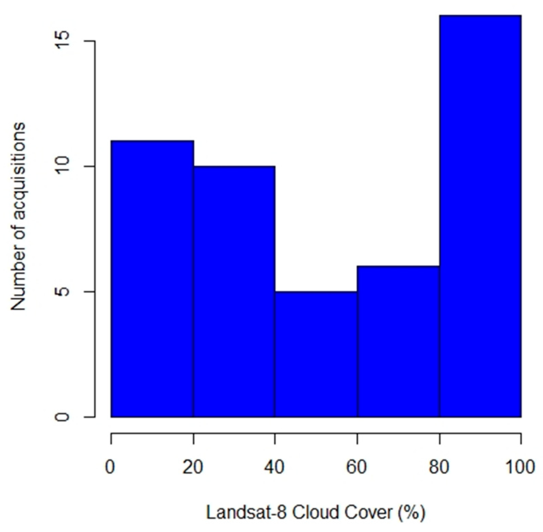
2.3. Landsat-8 Operational Land Imager (OLI) Data

The Landsat-8 Operational Land Imager (OLI) provides 30 m optical wavelength images with improved radiometry and geolocation compared to previous Landsat sensors [37]. The most recent Collection 1 Landsat images that are defined with per-pixel cloud and quality information [38] were used. In order to select contemporaneous imagery, two years of Landsat-8 OLI images acquired from July 2013 to August 2015, i.e., from one year before to one year after the airborne LiDAR data acquisitions, were considered. Only those OLI images that had <20% cloud cover (defined by the Collection 1 “land cloud cover” metadata) and that were cloud-free over the four LiDAR transects were selected. In total, out of 48 OLI images acquired over the two years, only two images, sensed 14 July 2013 (i.e., dry season) and 8 December 2014 (i.e., wet season) met these selection criteria. This is not surprising given the prevalence of cloud at the time of Landsat overpass that is evident in Figure 2.

The Landsat-8 OLI has nine 30 m reflective wavelength (435 nm to 2200 nm) bands. In this study OLI bands 3 (Green, ~560 nm), 4 (Red, ~655 nm), 5 (NIR, ~865 nm), 6 (Shortwave Infrared, ~1610 nm), and band 7 (Shortwave Infrared, ~2200 nm) were used. The two OLI blue bands were not used because of their sensitivity to atmospheric scattering [39,40]. The surface reflectance rather than top of atmosphere reflectance was used to minimize the effects of atmospheric contamination that can be particularly significant over the tropics due to high water vapor content and biogenic and pyrogenic aerosols. The surface reflectance imagery, were obtained from the United State Geographical Survey (USGS) website (https://earthexplorer.usgs.gov) and are derived using the Land Surface Reflectance Code (LaSRC) [40].

2.4. Aboveground Biomass Field Plot Validation Data

Field plot data used to validate AGB were collected in support of the Mai Ndombe Emission Reductions Program, a World Bank coordinated program (under the Forest Carbon Partnership Facility Carbon Fund) that aims to provide benefits for the local population while reducing greenhouse gas emissions from deforestation and forest degradation [41]. The field plots were in undisturbed primary forest [36]. The field plot data were collected November 2015 where the airborne LiDAR data had been flown the previous year (recall the LiDAR data were flown July and August 2014). The field plot data were collected in two of the study area LiDAR transects (the NE and SW transects illustrated in Figure 1a). In each transect, two field plots of one hectare situated <10 km apart were surveyed on the ground. Thus, there were four field plots in the study area.

Each field plot (1 ha) was divided into sixteen 25 m × 25 m (0.0625 ha) parcels. In each parcel, the diameter at breast height (1.3 m) for all trees with diameter >10 cm was measured. The species of each tree was identified by ecologists following the procedure described in [36] and the tree wood density was assigned using the Global Wood Density Database for tropical trees [7]. In cases where tree identification was not possible, the mean wood density of the plot was assigned. The tree AGB in each parcel was derived using a standard allometry model [10] as was undertaken by [36]:

$$\mathrm{AGB}=\frac{{10}^{-3}}{a}{{\displaystyle \sum }}_{i=1}^{n}exp(-1.803-0.976 e+0.976ln\left({\rho }_i\right)+2.673ln\left(d_i\right)-0.0299{\left(ln\left(d_i\right)\right)}^2)$$

(1)

where AGB is the estimated tree aboveground biomass in the parcel (Mg ha⁻¹), a is the parcel area (ha), d is the diameter at breast height of each tree in the parcel (cm), ρ is the wood density of each tree in the parcel (g cm^-3), n is the number of trees in the parcel, and e is an environmental stress parameter that depends on the seasonality of temperature, precipitation, and the climatic water deficit [10]. There were 16 parcels and so 16 AGB estimates were derived as (1) for each one hectare field plot, except for one field plot (located over the study area NE LiDAR transect) where there were 15 AGB estimates as no data was collected in one of its parcels. This provided a total of 63 AGB 25 m × 25 m parcel estimates.

No field measurements of the non-forest vegetation, i.e., grasses and shrubs, were made. The AGB of grasses and shrubs in tropical forests is not well documented, and although a minor fraction of tree AGB, post tropical forest disturbance (e.g., due to deforestation, degradation, or fire) grass, shrubs, and tree saplings grow rapidly [42]. However, in this study, only tree AGB was considered.

3. Methods

3.1. Forest Mask Classification

A 30 m forest mask was derived so that only the forest parts of the Landsat images would be considered. This is needed as about a quarter of the study area is composed of water and seasonally inundated soil (Figure 1). The Landsat images were acquired in the dry and wet seasons and so the lake level and the soil and cloud conditions were different between the images. In addition, the Landsat cloud and shadow mask was not always reliable, which has been observed by [43,44]. Therefore, in order to provide a reliable forest mask, a supervised random forest classification applied to both images was undertaken, which is a state of the practice land cover classification approach [45], and used to define forest, water, permanent wet soil (wet in both Landsat images), dry soil, cloud, and shadow classes. Training data were derived by visual interpretation of both Landsat images. Care was taken to ensure that the forest training pixels did not include mixed forest and non-forest pixels (e.g., over forest edges and small forest clearings) as they likely contain shrubs and grasses whose AGB is unknown. Care was also taken to select training samples across the study area and to ensure that the proportion selected among the different classes reflected the visually estimated study area class proportions in order to provide approximately similar class training portions as found by random sampling [46].

A total of 7280 training pixels of 30 m were collected composed of forest (67% of the pixels), water (25%), permanent wet soil (3%), dry soil (3%), cloud (1%), and shadow (1%) classes. The classification predictor variables were defined by the Landsat-8 OLI surface reflectance for bands 3, 4, 5, 6, and 7. In addition, normalized difference band ratios, defined like the normalized difference vegetation index (NDVI), for every possible two band combination of these bands were derived. This provided a total of 11 predictor variables. These bands and ratios have been used before for Landsat land cover classification [46,47,48].

The training data were used to develop a random forest classification tree using the default parameter settings, i.e., 500 trees were grown with each tree built using 63.2% of the training data selected randomly with replacement and three predictor variables (the square root of the number of predictor variables) randomly selected [49]. The random forest classification was applied to the 11 predictor variables at every 30 m study area pixel. The land cover classification was checked by visual comparison with the Landsat-8 OLI images and with Google Earth high resolution images. No formal quantitative per-pixel assessment of the classification accuracy was undertaken as the objective here was to develop a conservative forest mask used to discard non-forest pixels from the tree height and AGB mapping.

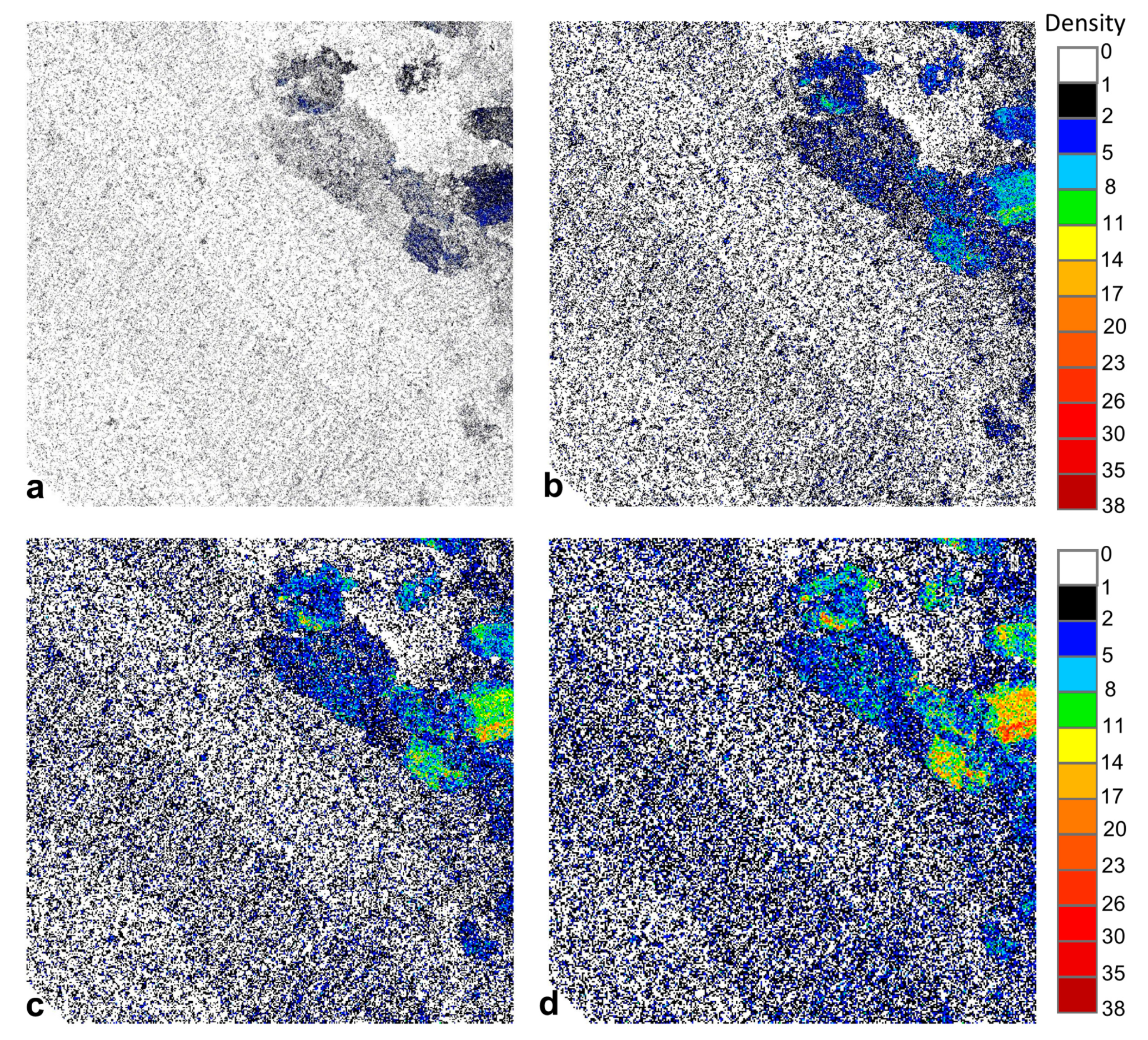
3.2. LiDAR Dominant Canopy Height Quantification

The data were processed using FUSION, a public software designed by the U.S. Forest Service to analyze LiDAR data [50]. The Landsat 30 m pixel grid was used to define a coordinate system.

First, the number of LiDAR ground returns in different sized grid cells (1 m, 2 m, 2.5 m, and 3 m side dimensions) aligned with the Landsat coordinate system were examined to determine an appropriate grid cell dimension for the subsequent processing. In the DRC national carbon mapping study undertaken by Xu et al. [36] a 2 m grid cell dimension was used. However, for the four study area transects, we found that a 2.5 m grid cell dimension was more appropriate as with smaller grid cells there were usually no ground returns in each grid cell. As an example, Figure 3 illustrates in detail the number of ground returns for the four different grid cell dimensions considered. The percentage of illustrated grid cells with no ground return data were 85%, 60.4%, 49.3%, and 39.7% for 1 m, 2 m, 2.5 m, and 3 m, grid cell dimensions, respectively. In Figure 3, the greatest ground return density is in the north east and occurs where there are no trees.

The discrete-return airborne LiDAR transect data categorized as ground returns were used to generate a 2.5 m ground height digital terrain model (DTM) by averaging the heights of the ground returns falling in each 2.5 m grid cell. Some DTM grid cells had no data (e.g., white in Figure 3) and the DTM gaps were interpolated from neighboring DTM grid cell values by natural neighbor interpolation that has been recommended for LiDAR processing [51] and has elegant interpolation properties, i.e., no parameters are used, the interpolated values are guaranteed to be within the range of the samples used and to pass through the input samples, and are smooth everywhere except at the locations of the input samples [39].

A canopy height model (CHM) was estimated by extracting the DTM height from the maximum first return height in each 2.5 m grid cell and only considering first returns with heights >1 m. This is a common approach in tropical forests if the LiDAR first returns are not particularly noisy [52,53,54,55].

The dominant canopy heights in 30 m grid cells aligned with the Landsat 30 m pixel grid were derived by taking the mean of the 2.5 m CHM values falling in each 30 m grid cell. The mean rather than another metric, such as the maximum or the median, was used as it provides a reliable representation of forest structure and has been used in other LiDAR based tropical forest studies [55,56,57]. The dominant canopy height was derived only for 30 m grid cells ≥75% covered by LiDAR data (i.e., containing ≥108 2.5 m canopy height values). This resulted in a proportion of the 30 m grid cells along the LiDAR transect edges being discarded from the analysis.

The above processing was also repeated independently for the LiDAR data falling over the 25 m × 25 m AGB field parcels (Section 2.4) and using the field plot corner locations to define a coordinate system. A 2.5 m DTM was generated, then, as above, any DTM gaps were filled by natural neighbor interpolation, canopy heights were estimated for each 2.5 m grid cell, and then the dominant canopy heights in the 25 m × 25 m grid cells falling over each 25 m × 25 m field plot parcel were derived.

3.3. Dominant Forest Canopy Height Prediction and Accuracy Assessment

The dominant forest canopy height was predicted at each Landsat 30 m pixel using the established non-parametric supervised random forest regression estimator [49]. Other researchers have also used this approach [16,22,55]. Only the 30 m pixels classified as forest (Section 3.1) were considered.

The response variable was defined by the 30 m dominant canopy height data (Section 3.2) sampled systematically every four pixels (120 m) north and south across each LiDAR transect. A four pixel sampling interval was used to reduce spatial autocorrelation effects that can introduce biases into the forest height prediction [58]. The four pixel sampling interval was selected beacause it is >100 m which is the distance that canopy heights in Mai Ndombe province were found to be significantly different from forest edge canopy heights [35].

A total of 5278 pixels with 30 m dominant canopy height response variables and 11 associated predictor variables were extracted. The predictor variables were defined by the Landsat-8 OLI surface reflectance for bands 3, 4, 5, 6, and 7. In addition, normalized difference band ratios, defined like the NDVI, for every possible two band combination of these bands were derived. The 5278 response and predictor values were divided into two equally sized portions, one portion was used to train the random forest regression and the other to test it. To ensure that a full range of forest canopy heights were used in both the training and testing, the following sampling procedure was used. The 5278 30 m dominant canopy height values were ranked into ascending canopy height order. Every second sample in the ranked list was selected as training data (n = 2639) and the remainder were used to define the test data (n = 2639). The dominant canopy heights for the training data ranged from 2.71 m to 43.99 m and for the test data ranged from 2.65 m to 42.71 m.

The random forest regression estimator was trained using the 2639 30 m dominant canopy height pixel training values and the 11 corresponding predictor values. The default random forest regression parameter settings were used, i.e., 500 trees were grown with each tree built using 63.2% of the training data selected at random with replacement and 3 predictor variables (one third the number of predictor variables) randomly selected [49]. The resulting random forest regression tree was applied to the 11 predictor variables at every forest mask Landsat-8 OLI pixel location to generate a 30 m dominant forest canopy height map.

The random forest regression prediction accuracy was assessed by application of the random forest regression tree to the 2639 test predictor variables. The resulting 2639 random forest regression predicted canopy heights were compared with the test 30 m dominant forest canopy heights and the Root Mean Square Error (RMSE) between them derived. In addition, scatterplots comparing the predicted and test 30 m dominant canopy heights were generated and Ordinary Least Squares (OLS) regressions between the data and the goodness of fit (R²) and regression confidence (p value) statistics were derived.

The above process was undertaken independently three times, using the Landsat-8 OLI predictor variables extracted from (a) only the dry season (14 July 2013) image, (b) only the wet season (8 December 2014) image, and (c) both images. This resulted in three dominant forest canopy height maps and three accuracy assessments.

3.4. Aboveground Biomass Mapping

The aboveground biomass (AGB) was derived at each 30 m pixel location with a dominant forest canopy height estimate as:

AGB = 1.88 h ^1.55

(2)

where AGB is the predicted aboveground biomass (Mg ha⁻¹) and h is the 30 m dominant forest canopy height predicted by the random forest regression tree (Section 3.3). This allometric equation was defined by Xu et al. [16] by statistically fitting 92 pairs of dominant canopy heights (derived using the same airborne LiDAR data as this study but extracted from more (33) LiDAR transects flown across the main forest types of the DRC) with field AGB estimates (derived as described in Section 2.4).

Three AGB maps were generated by application of Equation (2) to the 30 m dominant forest canopy height maps generated using predictor variables derived from the Landsat-8 OLI (a) dry season, (b) wet season, and (c) both images.

3.5. Aboveground Biomass Map Accuracy Assessment

The study area 30 m AGB maps were validated by comparing them with the field plot AGB data that were defined in 25 × 25 m parcels (Section 2.4). The Landsat pixels and field parcels have different sizes and are not aligned. Consequently, the 25 × 25 m parcel AGB estimates falling under each 30 × 30 m Landsat pixel location were weighted to derive an equivalent 30 m field AGB estimate as:

$${\mathrm{AGB}}^{30}=\frac{{{\displaystyle \sum }}_{i=1}^n{\mathrm{AGB}}_i^{25}{f}_i}{{{\displaystyle \sum }}_{i=1}^n{f}_i}$$

(3)

where ${AGB}^{30}$ is the 30 × 30 m AGB field estimate derived from the n (typically 4 but sometimes 2 or 1) parcel AGB estimates (${AGB}^{25}$) that fall under the 30 m Landsat pixel location, and $f_i$ is the fraction of the 30 × 30 m Landsat pixel area occupied by parcel i. As some Landsat 30 m pixels fall along the forest plot edges, and so include areas with no field AGB estimate information, i.e., ${\displaystyle \sum }_{i=1}^n{f}_i$≤1, only 30 m pixel locations with ${\displaystyle \sum }_{i=1}^n{f}_{i }$≥ 0.5 were considered. Thus, if a 30 m pixel was less than 50% covered by field plot parcels it was not considered.

The RMSE between ${AGB}^{30}$ and the corresponding mapped 30 m AGB values (Section 3.4) were derived. Scatterplots comparing these data were generated and OLS regressions between the data and the goodness of fit (R²) and regression confidence (p value) statistics were derived to quantify the correspondence of the data.

4. Results

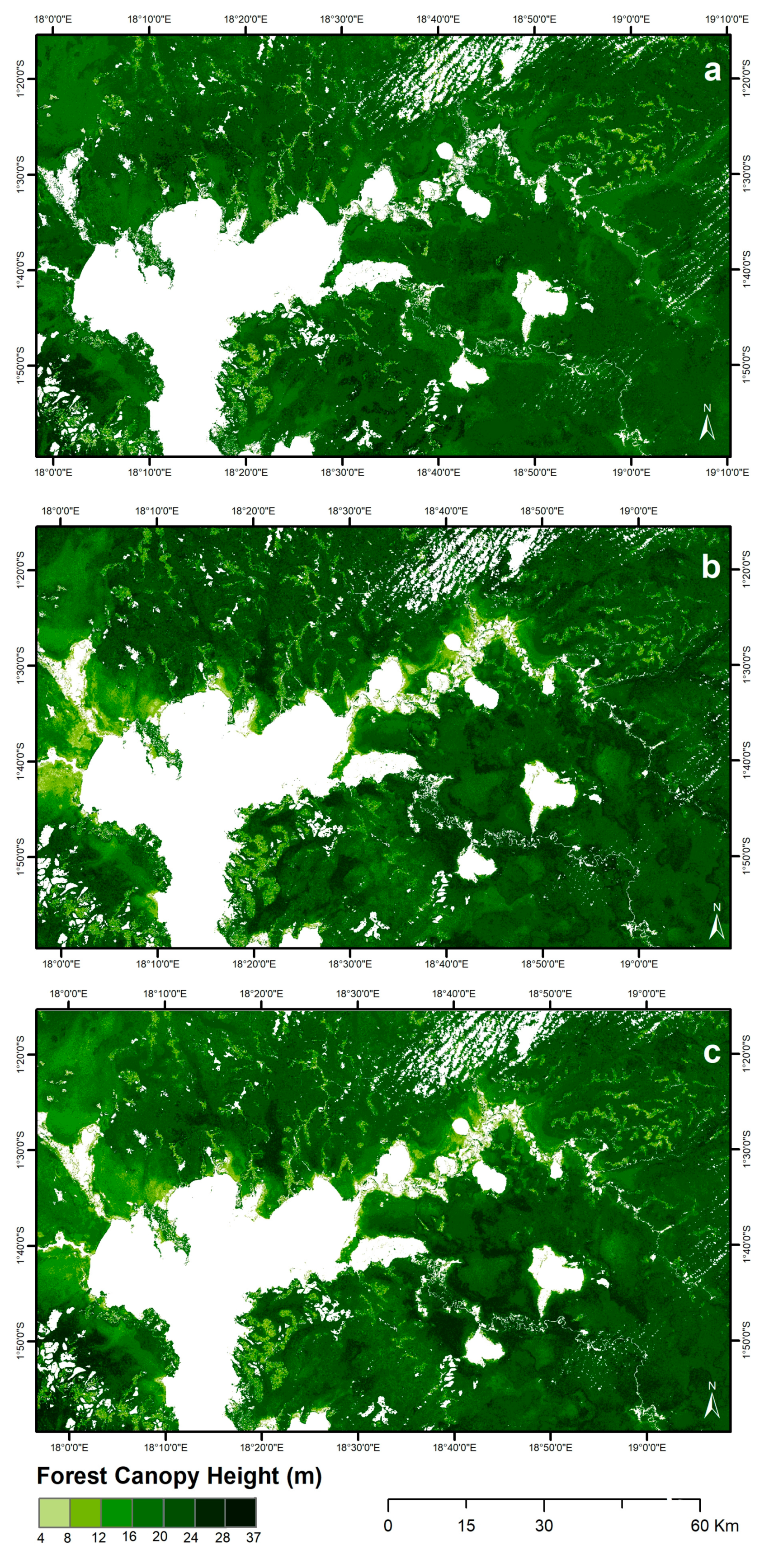
4.1. Dominant Forest Canopy Height Maps

Figure 4 shows the predicted 30 m dominant forest canopy heights for the study area derived using the Landsat-8 OLI predictor variables generated using (a) only the dry season, (b) only the wet season, and (c) both images. White shows the pixels that were classified as either water, permanent wet soil, dry soil, cloud, or shadow, and that were masked off from the subsequent AGB analysis. The masked off pixels include Lake Mai Ndombe evident in the wet season Landsat-8 OLI image (Figure 1a) and also capture most of the small rivers including streams with small axis dimensions greater than about half a 30 m pixel. Clouds and shadows located mostly in the North West that occurred in the dry season Landsat-8 OLI image are also apparent. Typically, forest edges and small forest clearings were classified as one of the non-forest classes (usually as wet soil or water) which is not a problem as these masked off pixels likely contain shrubs and grassed whose AGB is unknown.

The 30 m dominant forest canopy height maps derived using the predictor variables collected from the dry season (Figure 4a) and wet season (Figure 4b) Landsat-8 OLI images have a different evident spatial distribution. The differences are most evident around Lake Mai Ndombe and in the vicinity of several of the rivers. The mapped results derived using the predictor variables collected from both images (Figure 4c) tend to have intermediate or lower canopy heights. Despite these geographic differences, the mean 30 m dominant forest canopy height for the study area was similar between the three maps and was 20.6 m (Figure 4a), 20.8 m (Figure 4b), and 20.4 m (Figure 4c). The maximum 30 m dominant forest canopy height was 36.30 m, 37.22 m, and 37.23 m, respectively. The minimum 30 m dominant forest canopy height found in the three maps was very similar, within 0.01 m, and was approximately 4.0 m.

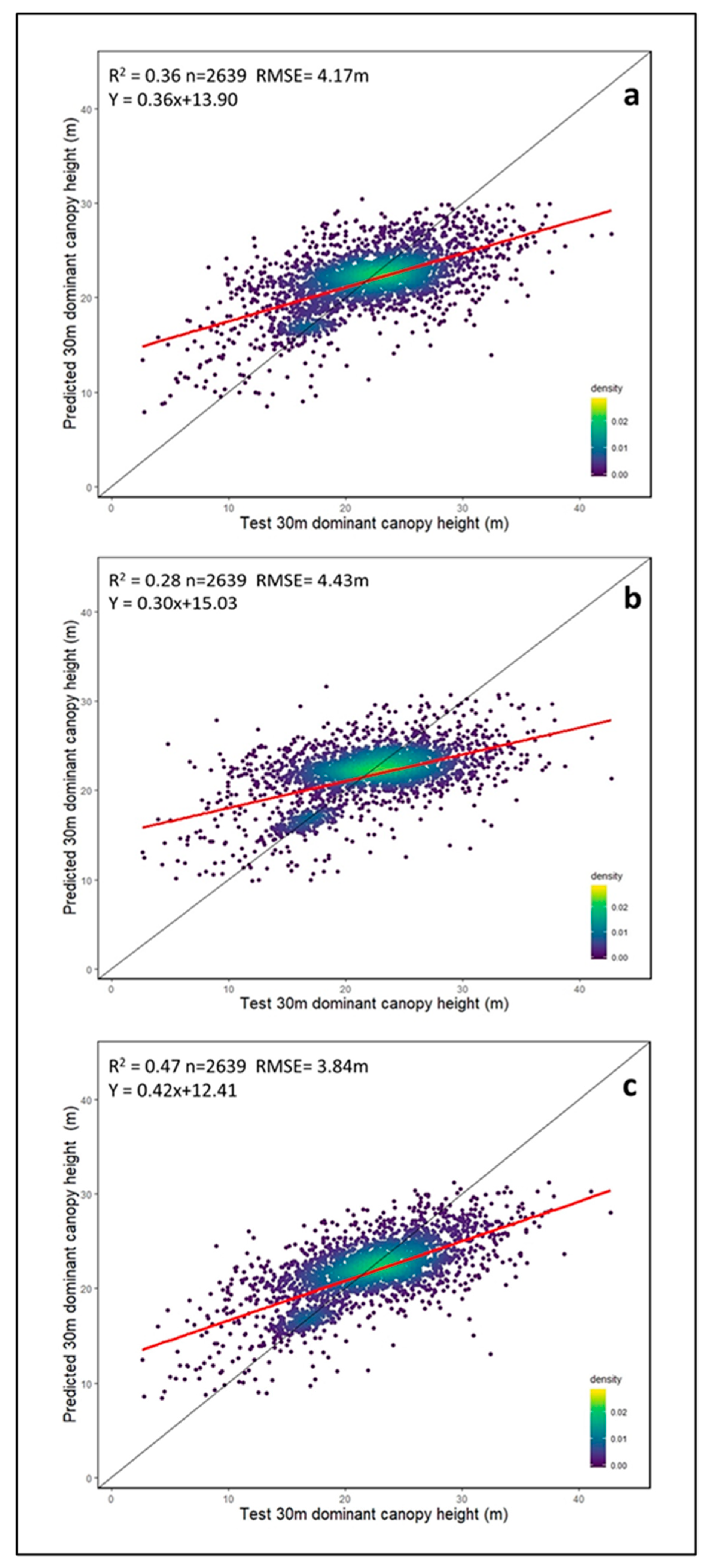
4.2. Dominant Forest Canopy Height Prediction Accuracy Assessment

The dominant forest canopy height prediction accuracy was assessed, as described in Section 3.3, by application of the random forest regression tree to the 2639 test pixels that were not used to train the tree. This was undertaken three times using the trees derived with Landsat-8 OLI predictor variables generated from (a) the dry season, (b) the wet season, and (c) both images. Figure 5 shows scatterplots comparing the test and the predicted 30 m dominant canopy height values. There are two clouds of dots evident in the scatterplots, the larger cloud corresponds to tall trees > 20 m present in the mature tropical evergreen forest parts of the four LiDAR transects, and the other corresponds to shorter forest canopies about 18 m high that occur predominantly around the Lake Mai Ndombe and often in the S.E. and S.W. LiDAR transects.

The OLS regressions of the plotted data are shown in red in Figure 5. In all three cases the regressions are significant (p values < 0.05) with slopes less than unity and intercepts > 12 m. The random forest regression underestimates and overestimates the heights for pixels dominated by tall and short trees, respectively. The predicted 30 m dominant canopy heights are similar to the test height values only for dominant canopy heights around 22 m. The wet season results (Figure 5b) have the lowest OLS regression R² (0.28) and the greatest RMSE (4.43 m). The dry season results (Figure 5a) are slightly improved with an 0.36 R² and a 4.17 m RMSE. The prediction accuracy is best when both the Landsat-8 OLI images were used (Figure 5c) with an 0.47 R², a 3.84 m RMSE, and the OLS regression slope is closer to unity (0.42) and the intercept is closer to zero (12.41 m). This 3.84 m RMSE value corresponds to about 17% of the mean of the 2639 test pixel canopy height values (22 m). These results indicate that using both the dry and wet season Landsat-8 OLI images provides more accurate dominant canopy height prediction.

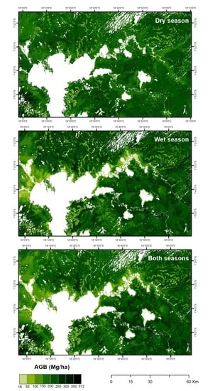
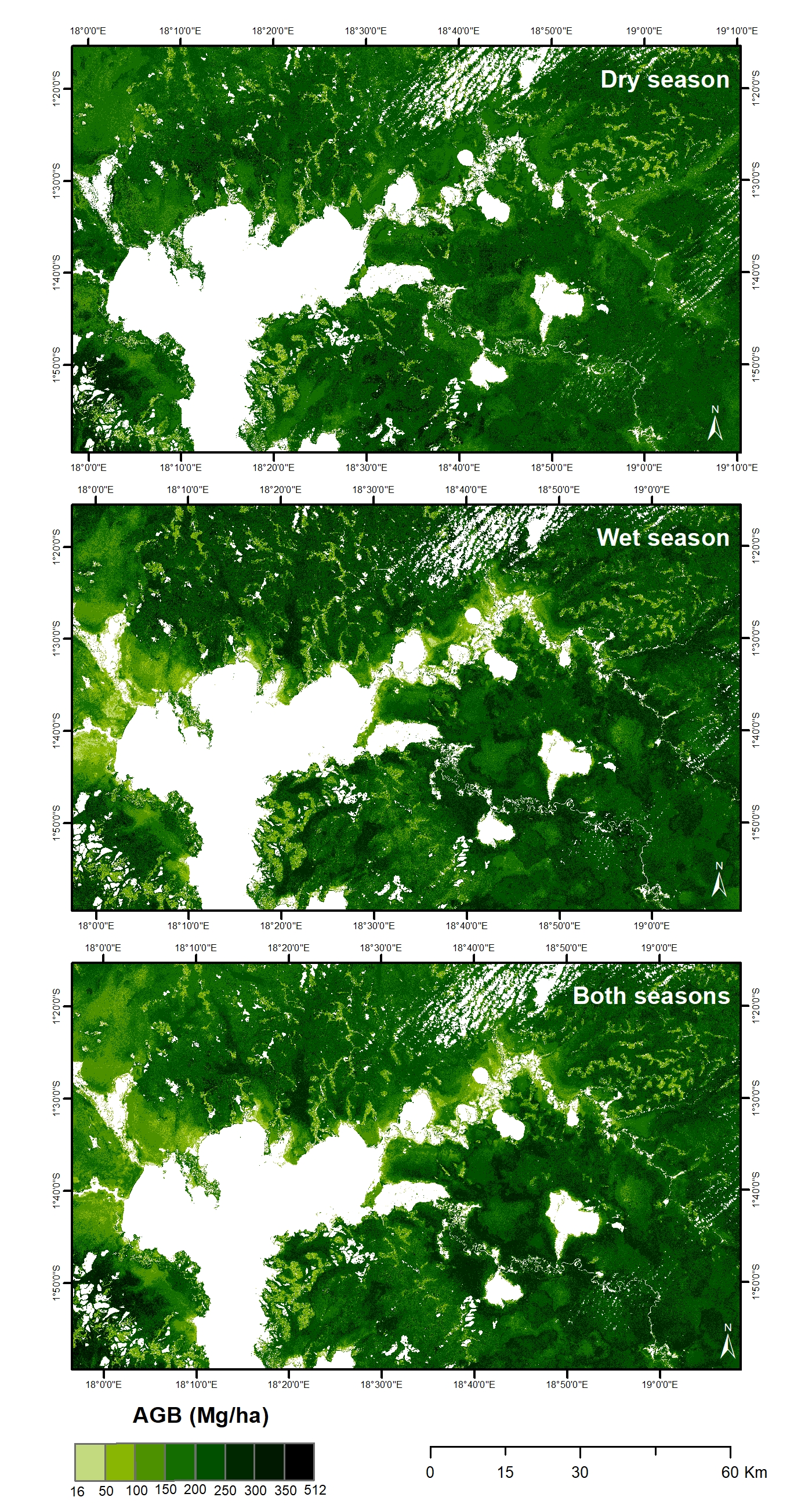
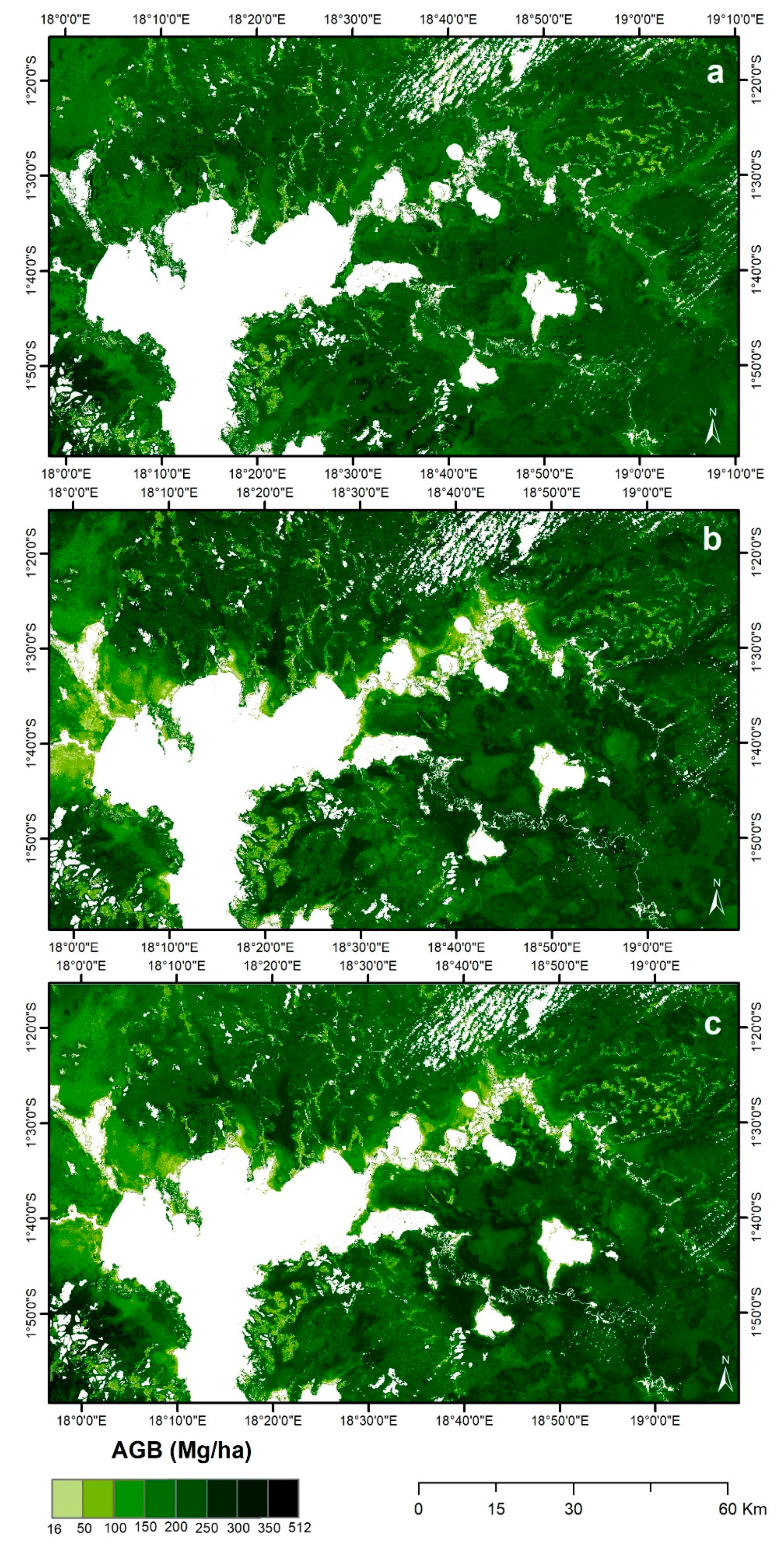
4.3. Aboveground Biomass Maps

Figure 6 shows the 30 m AGB biomass maps derived from the 30 m dominant forest canopy height maps (Figure 4) using Equation (2). The same broad patterns as the dominant forest canopy height maps are observed, which is expected given that the AGB is proportional to the dominant canopy height.

The mean study area AGB was 206 Mg ha⁻¹, 211 Mg ha⁻¹, and 204 Mg ha⁻¹ for the AGB maps generated using the dry season, wet season and both images dominant forest canopy height maps, respectively. The maximum AGB was found at the 30 m pixels with greatest dominant canopy height and was 493.5 Mg ha⁻¹ (tree height 36.3 m), 511.8 Mg ha⁻¹ (tree height 37.22 m), and 511.8 Mg ha⁻¹ (tree height 37.23 m) for the dry season, wet season, and both image maps, respectively. The minimum 30 m AGB among the three maps was very similar, within 0.01 Mg ha⁻¹, and was approximately 16 Mg ha⁻¹.

4.4. Aboveground Biomass Validation

Figure 7 shows scatterplots comparing the 30 m AGB derived from the remotely sensed data (Figure 6) and the 30 m area weighted AGB field estimates (${\mathrm{AGB}}^{30}$) over the four one-hectare field plots. The three scatterplots compare the same ${\mathrm{AGB}}^{30}$ with AGB predicted using forest canopy heights generated from the dry season (Figure 7a), wet season (Figure 7b), and both (Figure 7c) Landsat-8 OLI images. There were 63 AGB 25 m × 25 m parcel estimates but after the area weighting to 30 m (Equation (3)) and application of the constraint that 50% of the 25 m × 25 m parcels with AGB estimates must fall under a 30 m pixel (Section 3.5), there were 43 pairs of values. The 43 plotted values are color coded to designate which of the four field plots the ${\mathrm{AGB}}^{30}$ were derived from. They illustrate that two of the field plots (purple and green) had higher ${\mathrm{AGB}}^{30}$ and that there was a wide range of values from about 96 Mg ha⁻¹ to 503 Mg ha⁻¹. However, this range is smaller than present in the estimated 30 m AGB study area maps shown in Figure 6 that had AGB that varied from approximately 16 to 512 Mg ha⁻¹.

The OLS regressions of the plotted data are shown in red and were insignificant for the dry (Figure 7a) and wet (Figure 7b) season derived image results (p values > 0.05) with small R² values, of 0.05 and 0.07, respectively. Conversely, the OLS regression results for the AGB estimated using the dominant forest canopy heights derived from both Landsat images (Figure 7c) was more significant (p = 0.03) with a 0.11 R² value, and a slope closer to unity (0.135) and an intercept closer to zero (193 Mg ha⁻¹). The RMSE values for the wet and dry season results were 92.43 Mg ha⁻¹ and 87.76 Mg ha⁻¹, respectively, and smaller, 83.77 Mg ha⁻¹, for the combined image results. The 83.77 Mg ha⁻¹ RMSE value corresponds to about 41% of the mean study area mapped AGB (204 Mg ha⁻¹) (Figure 6c). However, clearly, the mapped AGB is over-estimated below about 225 Mg ha⁻¹ and under-estimated above this value (Figure 7c).

5. Discussion

The AGB of the Congo Basin forest has been poorly documented due to a lack of inventory data and research [59]. Recently, airborne LiDAR and Landsat-8 OLI data have been used to map tree height and AGB across all of the Congo Basin [16]. Cloud cover at the time of Landsat overpass can be high (e.g., Figure 2), reducing the ability to obtain cloud-free imagery needed to undertake the mapping. Consequently, Xu et al. [16] defined Landsat predictor variables by the medians (i.e., 50th percentiles) of the red, NIR, and the two shortwave Landsat-8 OLI reflective wavelength bands acquired over three years. Thus, the predictor variables at adjacent pixel locations may have been selected from different years and seasons which is an issue if the forest and the Landsat forest reflectance changed between years and seasons. However, the detailed processing and results of this study show, on average at the study area level, no great difference between the dry and wet season dominant canopy height and AGB results, i.e., little sensitivity to the seasonality of the Landsat imagery used. This is discussed below.

The dominant forest canopy heights and AGB estimated from the dry season Landsat-8 OLI image were on average marginally lower than those estimated from the wet season image. The RMSE between the mapped and 2639 independent test 30 m dominant canopy heights was 4.17 m (dry season) and 4.43 m (wet season) and corresponds to 20.2% and 21.2% of the mean study area mapped dominant canopy heights that were 20.6 m (dry season) and 20.8 m (wet season). The RMSE between the mapped and 43 independent field based 30 m AGB estimates was 87.76 Mg ha⁻¹ (dry season) and 92.43 Mg ha⁻¹ (wet season) and corresponds to 42.6% and 43.8% of the mean study area mapped AGB that was 206 Mg ha⁻¹ (dry season) and 211 Mg ha⁻¹ (wet season).

There were seasonal geographic differences between the mapped dominant canopy height (Figure 4) and the AGB (Figure 6) results, in particular around Lake Mai Ndombe and in the vicinity of several of the rivers. The reasons for this are complex but may be due to seasonal vegetation condition and surface differences. For example, although the Landsat 30 m forest mask was derived conservatively, sub-pixel disturbed forest patches, and degraded forest areas with reduced live tree cover, may include shrubs and saplings that exhibit greater seasonal reflectance differences than elsewhere in the forest. In addition, in these regions, wet season flood water may have been observable at Landsat resolution through the forest canopy.

The pre-processing applied to the LiDAR and Landsat-8 OLI data were state of the practice. However, the difference between the seasonal results may have been affected by Landsat bi-directional reflectance distribution (BRDF) effects. Landsat BRDF variations are smaller than in wider field of view satellite optical wavelength data and occur due to changes in the view geometry across the image swath and to temporal changes in the solar geometry [60,61]. The two Landsat-8 OLI images were not corrected for BRDF effects because they were both sensed from the same orbit and so have similar view geometry. The solar zenith angle at the center of each image was 35.85° and 32.30° for the dry and wet season images, respectively. This 3.55° solar zenith difference is small compared to the 15° Landsat field of view although variations of this magnitude can cause small reflectance variations [61]. Use of both the dry and wet season Landsat-8 OLI images provided the lowest RMSE value (3.84 m) between the predicted and test dominant forest canopy heights, corresponding to 18.8% of the mean study area mapped tree height (20.4 m) derived using both images. This 18.8% RMSE is quite small and was not particularly expected as many of the study area forest Landsat pixels have high NDVI (~0.8) which is indicative of “saturated vegetation” reflectance conditions. Typically, the NDVI saturates with increased Leaf Area Index (LAI) above about LAI ~3.0 [62] and Congo basin tropical evergreen rainforest has LAI > 5 [63,64]. Presumably, despite this potential saturation issue, other factors related to the dominant forest canopy height could be discriminated by the random forest regression model using the wet and dry season Landsat-8 OLI images. Notably, the R² value was not particularly high (0.47) but the regression was significant (p < 0.001), indicating that the regression fit model illustrated in Figure 5c is better than not having a model. Moreover, the R² is comparable to other recent study results, for example, Staben et al. [22] reported a 0.49 R² between mapped and predicted forest canopy height in the Northern territory, Australia.

Using both Landsat-8 OLI images provided the most accurate AGB prediction and the lowest RMSE value (83.77 Mg ha⁻¹) between predicted and field estimated AGB. This was expected because the AGB was derived as an allometric function of the dominant canopy height which was most accurately predicted using both Landsat-8 OLI images. Although the R² was low (0.11) the regression was significant (p < 0.03), indicating that the regression fit model illustrated in Figure 7c is better than not having a model. As noted earlier, the range of the field plot derived AGB (~96 Mg ha⁻¹ to 503 Mg ha⁻¹) is smaller than the range of the study area estimated 30 m AGB (~16 to 512 Mg ha⁻¹), and the field plot data were available at only four 1 ha sites, which may reduce the representativeness of the validation results. However, the 83.77 Mg ha⁻¹ AGB RMSE is comparable to the 89.83 Mg ha⁻¹ RMSE value reported by Xu et al. [16] and corresponds to about ~40% of the reported mean Congo Forest AGB. This is quite a high error but is not surprising as we found that the dominant canopy heights were under-estimated for trees > ~25 m and over-estimated for trees < ~18 m (Figure 5). Similarly, the AGB was over-estimated below about 225 Mg ha⁻¹ and under-estimated above this value (Figure 7).

The magnitude of the estimated mean study area AGB derived using both Landsat-8 OLI images (204 Mg ha⁻¹) is similar to that reported in other Congo Basin forest studies. For example, Baccini et al. [59] reported 216 Mg ha⁻¹ for the evergreen rainforest of Central Africa, Silva et al. [65] reported 223 Mg ha⁻¹ for Lope National Park in Central Gabon, and Xu et al. [16] reported 231 Mg ha⁻¹ for all the DRC. Similarly, the magnitude of the maximum study area AGB derived using both Landsat-8 OLI images (511.8 Mg ha⁻¹) was comparable to the maximum Congo Basin forest AGB reported by Silva et al. [65] and Xu et al. [16]. Thus, the maximum AGB that a hectare of Congo basin forest can store is about 500 Mg, which demonstrates the importance of these forests for carbon storage.

The predicted dominant canopy height results were derived using LiDAR transect training data acquired in July and August 2014, i.e., up to 12 and 13 months, respectively, after the dry season Landsat image acquisition, and up to 6 and 5 months, respectively, before the wet season Landsat image acquisition. The reliability of the dominant canopy height prediction will be reduced if the forest within the transects was disturbed in these periods. However, given the paucity of cloud-free satellite data we have no way to check this. The field plot data used to derive the AGB validation data were collected November 2015, i.e., 11 and 28 months after the wet and dry season Landsat images, respectively. The field plot data were collected in undisturbed primary forest and so are unlikely to have been subsequently disturbed but, again, we have not way to check this definitively. These issues underscore the difficulty in mapping and validating DRC dominant forest canopy height and AGB.

The degree to which AGB estimation can be improved using optical wavelength data is unknown. Further research to examine the effects of using additional satellite data, such as the Landsat-like Sentinel-2 data [66], to see if the height estimation can be improved, is warranted. Using improved allometry [8] and recent spaceborne LiDAR data [67] is also warranted.

6. Conclusions

The sensitivity of airborne LiDAR and Landsat-8 OLI based dominant canopy height and AGB 30 m mapping was assessed with respect to the season of Landsat acquisition for a ~10,000 km² Congo Basin tropical forest study area. Experiments were undertaken independently three times to map and assess the 30 m dominant canopy height and AGB using (i) only a wet season Landsat-8 image, (ii) only a dry season Landsat-8 image, and (iii) both images. The images were predominantly cloud-free. A random forest regression estimator was used to predict and assess the 30 m dominant canopy height using LiDAR derived test and training data. The AGB was mapped using an allometric model parameterized with the dominant canopy height and was assessed by comparison with 43 field based 30 m AGB estimates.

The most accurate results were obtained using both the dry and wet season Landsat-8 OLI images together. The RMSE between the mapped and test 30 m dominant canopy heights was 3.84 m, and the RMSE between the mapped and field based AGB estimates was 83.77 Mg ha⁻¹. These RMSE values correspond to 18.8% of the mean study area mapped tree height (20.4 m) and to 41% of the mean study area mapped AGB (204 Mg ha⁻¹). The mean study area mapped AGB is similar to that reported in other Congo Basin forest studies [16,59,65].

At the study area level there was little sensitivity to the seasonality of the Landsat imagery used. The study area mean dominant canopy height and AGB values were similar between seasons, within 0.19 m and 5 Mg ha⁻¹, respectively, and the RMSE between the mapped and test 30 m dominant canopy heights was 4.17 m (dry season) and 4.43 m (wet season), and the RMSE between the mapped and field based AGB estimates was 87.76 Mg ha⁻¹ (dry season) and 92.43 Mg ha⁻¹ (wet season).

The degree to which AGB estimation can be improved using temporally richer optical wavelength data is unknown due to difficulties in obtaining cloud-free imagery. These results suggest that (i) using a single cloud-free Landsat-8 OLI image may be sufficient for airborne LiDAR and Landsat-8 OLI based dominant canopy height and AGB 30 m mapping in the Congo Basin tropical forest, but (ii) using Landsat imagery from different seasons is preferred to improve tropical forest inventories in the Congo Basin forest.

References

1. Houghton, R.A. Aboveground Forest Biomass and the Global Carbon Balance. Glob. Chang. Biol. 2005, 11, 945–958. [Google Scholar] [CrossRef]
2. Meyer, V.; Saatchi, S.; Ferraz, A.; Xu, L.; Duque, A.; Garcia, M.; Chave, J. Forest degradation and biomass loss along the Choco region of Colombia. Carbon Balance Manag. 2019, 14, 2. [Google Scholar] [CrossRef] [PubMed]
3. Hubau, W.; Lewis, S.L.; Phillips, O.L.; Affum-Baffoe, K.; Beeckman, H.; Cuni-Sanchez, A.; Daniels, A.K.; Ewango, C.E.N.; Fauset, S.; Mukinzi, J.M.; et al. Asynchronous carbon sink saturation in African and Amazonian tropical forests. Nature 2020, 579, 80–87. [Google Scholar] [CrossRef] [PubMed] [Green Version]
4. Clark, D.B.; Clark, D.A. Landscape-scale variation in forest structure and biomass in a tropical rain forest. For. Ecol. Manag. 2000, 137, 185–198. [Google Scholar] [CrossRef]
5. Saatchi, S.; Marlier, M.; Chazdon, R.L.; Clark, D.B.; Russell, A.E. Impact of spatial variability of tropical forest structure on radar estimation of aboveground biomass. Remote Sens. Environ. 2011, 115, 2836–2849. [Google Scholar] [CrossRef]
6. Ferraz, A.; Saatchi, S.; Mallet, C.; Meyer, V. Lidar detection of individual tree size in tropical forests. Remote Sens. Environ. 2016, 183, 318–333. [Google Scholar] [CrossRef]
7. Chave, J.; Andalo, C.; Brown, S.; Cairns, M.A.; Chambers, J.Q.; Eamus, D.; Folster, H.; Fromard, F.; Higuchi, N.; Kira, T.; et al. Tree allometry and improved estimation of carbon stocks and balance in tropical forests. Oecologia 2005, 145, 87–99. [Google Scholar] [CrossRef]
8. Skole, D.L.; Samek, J.H.; Smalligan, M.J. Implications of allometry. Proc. Natl. Acad. Sci. USA 2011, 108, E12. [Google Scholar] [CrossRef] [Green Version]
9. Clark, D.B.; Kellner, J.R. Tropical forest biomass estimation and the fallacy of misplaced concreteness. J. Veg. Sci. 2012, 23, 1191–1196. [Google Scholar] [CrossRef]
10. Chave, J.; Rejou-Mechain, M.; Burquez, A.; Chidumayo, E.; Colgan, M.S.; Delitti, W.B.; Duque, A.; Eid, T.; Fearnside, P.M.; Goodman, R.C.; et al. Improved allometric models to estimate the aboveground biomass of tropical trees. Glob. Chang. Biol. 2014, 20, 3177–3190. [Google Scholar] [CrossRef]
11. Foody, G.M.; Boyd, D.S.; Cutler, M.E.J. Predictive relations of tropical forest biomass from Landsat TM data and their transferability between regions. Remote Sens. Environ. 2003, 85, 463–474. [Google Scholar] [CrossRef]
12. Lu, D. Aboveground biomass estimation using Landsat TM data in the Brazilian Amazon. Int. J. Remote Sens. 2005, 26, 2509–2525. [Google Scholar] [CrossRef]
13. Disney, M.I.; Boni Vicari, M.; Burt, A.; Calders, K.; Lewis, S.L.; Raumonen, P.; Wilkes, P. Weighing trees with lasers: Advances, challenges and opportunities. Interface Focus 2018, 8, 20170048. [Google Scholar] [CrossRef] [Green Version]
14. Csillik, O.; Kumar, P.; Mascaro, J.; O’Shea, T.; Asner, G.P. Monitoring tropical forest carbon stocks and emissions using Planet satellite data. Nat. Sci. Rep. 2019, 9, 17831. [Google Scholar] [CrossRef] [Green Version]
15. Hansen, M.C.; Krylov, A.; Tyukavina, A.; Potapov, P.V.; Turubanova, S.; Zutta, B.; Ifo, S.; Margono, B.; Stolle, F.; Moore, R. Humid tropical forest disturbance alerts using Landsat data. Environ. Res. Lett. 2016, 11, 034008. [Google Scholar] [CrossRef]
16. Xu, L.; Saatchi, S.S.; Shapiro, A.; Meyer, V.; Ferraz, A.; Yang, Y.; Bastin, J.F.; Banks, N.; Boeckx, P.; Verbeeck, H.; et al. Spatial Distribution of Carbon Stored in Forests of the Democratic Republic of Congo. Nat. Sci. Rep. 2017, 7, 15030. [Google Scholar] [CrossRef] [Green Version]
17. Matasci, G.; Hermosilla, T.; Wulder, M.A.; White, J.C.; Coops, N.C.; Hobart, G.W.; Zald, H.S.J. Large-area mapping of Canadian boreal forest cover, height, biomass and other structural attributes using Landsat composites and lidar plots. Remote Sens. Environ. 2018, 209, 90–106. [Google Scholar] [CrossRef]
18. Asner, G.P. Cloud cover in Landsat observations of the Brazilian Amazon. Int. J. Remote Sens. 2001, 22, 3855–3862. [Google Scholar] [CrossRef]
19. Lindquist, E.J.; Hansen, M.C.; Roy, D.P.; Justice, C.O. The suitability of decadal image data sets for mapping tropical forest cover change in the Democratic Republic of Congo: Implications for the global land survey. Int. J. Remote Sens. 2008, 29, 7269–7275. [Google Scholar] [CrossRef]
20. Kovalskyy, V.; Roy, D.P. The global availability of Landsat 5 TM and Landsat 7 ETM+ land surface observations and implications for global 30m Landsat data product generation. Remote Sens. Environ. 2013, 130, 280–293. [Google Scholar] [CrossRef] [Green Version]
21. Dommo, A.; Philippon, N.; Vondou, D.A.; Sèze, G.; Eastman, R. The June–September Low Cloud Cover in Western Central Africa: Mean Spatial Distribution and Diurnal Evolution, and Associated Atmospheric Dynamics. J. Clim. 2018, 31. [Google Scholar] [CrossRef]
22. Staben, G.; Lucieer, A.; Scarth, P. Modelling LiDAR derived tree canopy height from Landsat TM, ETM+ and OLI satellite imagery—A machine learning approach. Int. J. Appl. Earth Obs. Geoinf. 2018, 73, 666–681. [Google Scholar] [CrossRef]
23. Myneni, R.B.; Yang, W.; Nemani, R.R.; Huete, A.R.; Dickinson, R.E.; Knyazikhin, Y.; Didan, K.; Fu, R.; Negron Juarez, R.I.; Saatchi, S.; et al. Large seasonal swings in leaf area of Amazon rainforests. Proc. Natl. Acad. Sci. USA 2007, 104, 4820–4823. [Google Scholar] [CrossRef] [Green Version]
24. Brando, P.M.; Goetz, S.J.; Baccini, A.; Nepstad, D.C.; Beck, P.S.; Christman, M.C. Seasonal and interannual variability of climate and vegetation indices across the Amazon. Proc. Natl. Acad. Sci. USA 2010, 107, 14685–14690. [Google Scholar] [CrossRef] [Green Version]
25. Yang, J.; Tian, H.; Pan, S.; Chen, G.; Zhang, B.; Dangal, S. Amazon drought and forest response: Largely reduced forest photosynthesis but slightly increased canopy greenness during the extreme drought of 2015/2016. Glob. Chang. Biol. 2018, 24, 1919–1934. [Google Scholar] [CrossRef]
26. Manoli, G.; Ivanov, V.Y.; Fatichi, S. Dry-Season Greening and Water Stress in Amazonia: The Role of Modeling Leaf Phenology. J. Geophys. Res. Biogeosci. 2018, 123, 1909–1926. [Google Scholar] [CrossRef]
27. Egorov, A.; Roy, D.; Zhang, H.; Hansen, M.; Kommareddy, A. Demonstration of Percent Tree Cover Mapping Using Landsat Analysis Ready Data (ARD) and Sensitivity with Respect to Landsat ARD Processing Level. Remote Sens. 2018, 10, 209. [Google Scholar] [CrossRef] [Green Version]
28. Samba, G.; Nganga, D.; Mpounza, M. Rainfall and temperature variations over Congo-Brazzaville between 1950 and 1998. Theor. Appl. Climatol. 2007, 91, 85–97. [Google Scholar] [CrossRef]
29. Einzmann, K.; Haarpaintner, J.; Larsen, Y. Forest monitoring in Congo Basin with combined use of SAR C- & L-band. In Proceedings of the 2012 IEEE International Geoscience and Remote Sensing Symposium, Munich, Germany, 22–27 July 2012; pp. 6573–6576. [Google Scholar]
30. Bwangoy, J.-R.B.; Hansen, M.C.; Roy, D.P.; Grandi, G.D.; Justice, C.O. Wetland mapping in the Congo Basin using optical and radar remotely sensed data and derived topographical indices. Remote Sens. Environ. 2010, 114, 73–86. [Google Scholar] [CrossRef]
31. Mayaux, P.; De Grandi, G.; Malingreau, J.P. Central African Forest Cover Revisited. Remote Sens. Environ. 2000, 71, 183–196. [Google Scholar] [CrossRef]
32. Bwangoy, J.-R.B.; Hansen, M.C.; Potapov, P.; Turubanova, S.; Lumbuenamo, R.S. Identifying nascent wetland forest conversion in the Democratic Republic of the Congo. Wetl. Ecol. Manag. 2012, 21, 29–43. [Google Scholar] [CrossRef]
33. Molinario, G.; Hansen, M.C.; Potapov, P.V. Forest cover dynamics of shifting cultivation in the Democratic Republic of Congo: A remote sensing-based assessment for 2000–2010. Environ. Res. Lett. 2015, 10, 094009. [Google Scholar] [CrossRef]
34. Zhuravleva, I.; Turubanova, S.; Potapov, P.; Hansen, M.; Tyukavina, A.; Minnemeyer, S.; Laporte, N.; Goetz, S.; Verbelen, F.; Thies, C. Satellite-based primary forest degradation assessment in the Democratic Republic of the Congo, 2000–2010. Environ. Res. Lett. 2013, 8, 024034. [Google Scholar] [CrossRef] [Green Version]
35. Shapiro, A.C.; Aguilar-Amuchastegui, N.; Hostert, P.; Bastin, J.F. Using fragmentation to assess degradation of forest edges in Democratic Republic of Congo. Carbon Balance Manag. 2016, 11, 11. [Google Scholar] [CrossRef]
36. Xu, L.; Saatchi, S.S.; Shapiro, A.; Meyer, V.; Ferraz, A.; Yang, Y.; Bastin, J.-F.; Banks, N.; Boeckx, P.; Verbeeck, H.; et al. Spatial Distribution of Carbon Stored in Forests of the Democratic Republic of Congo. Supplemental information. Available online: https://static-content.springer.com/esm/art%3A10.1038%2Fs41598-017-15050-z/MediaObjects/41598_2017_15050_MOESM1_ESM.pdf (accessed on 24 April 2020).
37. Roy, D.P.; Wulder, M.A.; Loveland, T.R.; Woodcock, C.E.; Allen, R.G.; Anderson, M.C.; Helder, D.; Irons, J.R.; Johnson, D.M.; Kennedy, R.; et al. Landsat-8: Science and product vision for terrestrial global change research. Remote Sens. Environ. 2014, 145, 154–172. [Google Scholar] [CrossRef] [Green Version]
38. Dwyer, J.L.; Roy, D.P.; Sauer, B.; Jenkerson, C.B.; Zhang, H.K. Analysis Ready Data: Enabling Analysis of the Landsat Archive. Remote Sens. 2018, 10, 19. [Google Scholar]
39. Ju, J.; Roy, D.P.; Vermote, E.; Masek, J.; Kovalskyy, V. Continental-scale validation of MODIS-based and LEDAPS Landsat ETM+ atmospheric correction methods. Remote Sens. Environ. 2012, 122, 175–184. [Google Scholar] [CrossRef] [Green Version]
40. Vermote, E.; Justice, C.; Claverie, M.; Franch, B. Preliminary analysis of the performance of the Landsat 8/OLI land surface reflectance product. Remote Sens. Environ. 2016, 185, 46–56. [Google Scholar] [CrossRef]
41. World-Bank. Emission Reduction Program; World Bank/Forest Carbon Partnership Facility: Washington, DC, USA, 2016; pp. 1–297. [Google Scholar]
42. Souza, C.M.; Roberts, D.A.; Monteiro, A.L. Multitemporal Analysis of Degraded Forest in the Southern Brazilian Amazon. Earth Interact. 2005, 9, 1–25. [Google Scholar] [CrossRef] [Green Version]
43. Qiu, S.; Lin, Y.; Shang, R.; Zhang, J.; Ma, L.; Zhu, Z. Making Landsat Time Series Consistent: Evaluating and Improving Landsat Analysis Ready Data. Remote Sens. 2019, 11, 51. [Google Scholar] [CrossRef] [Green Version]
44. Egorov, A.; Roy, D.; Zhang, H.; Li, Z.; Yan, L.; Huang, H. Landsat 4, 5 and 7 (1982 to 2017) Analysis Ready Data (ARD) Observation Coverage over the Conterminous United States and Implications for Terrestrial Monitoring. Remote Sens. 2019, 11, 447. [Google Scholar] [CrossRef] [Green Version]
45. Wulder, M.A.; Coops, N.C.; Roy, D.P.; White, J.C.; Hermosilla, T. Land cover 2.0. Int. J. Remote Sens. 2018, 39, 4254–4284. [Google Scholar] [CrossRef] [Green Version]
46. Zhang, H.K.; Roy, D.P. Using the 500 m MODIS land cover product to derive a consistent continental scale 30 m Landsat land cover classification. Remote Sens. Environ. 2017, 197, 15–34. [Google Scholar] [CrossRef]
47. Hansen, M.C.; Egorov, A.; Roy, D.P.; Potapov, P.; Ju, J.; Turubanova, S.; Kommareddy, I.; Loveland, T.R. Continuous fields of land cover for the conterminous United States using Landsat data: First results from the Web-Enabled Landsat Data (WELD) project. Remote Sens. Lett. 2011, 2, 279–288. [Google Scholar] [CrossRef]
48. Yan, L.; Roy, D.P. Improved time series land cover classification by missing-observation-adaptive nonlinear dimensionality reduction. Remote Sens. Environ. 2015, 158, 478–491. [Google Scholar] [CrossRef] [Green Version]
49. Breiman, L. Random Forests. Mach. Learn. 2001, 45, 5–32. [Google Scholar] [CrossRef] [Green Version]
50. McGaughey, R.J. FUSION LDV: Software for LiDAR Data Analysis and Visualization; U.S. Department of Agriculture, Forest Service, Pacific Northwest Research Station, University of Washington: Seattle, WA, USA, 2016; pp. 1–212. [Google Scholar]
51. Bater, C.W.; Coops, N.C. Evaluating error associated with lidar-derived DEM interpolation. Comput. Geosci. 2009, 35, 289–300. [Google Scholar] [CrossRef]
52. Asner, G.P.; Mascaro, J. Mapping tropical forest carbon: Calibrating plot estimates to a simple LiDAR metric. Remote Sens. Environ. 2014, 140, 614–624. [Google Scholar] [CrossRef]
53. Leitold, V.; Keller, M.; Morton, D.C.; Cook, B.D.; Shimabukuro, Y.E. Airborne lidar-based estimates of tropical forest structure in complex terrain: Opportunities and trade-offs for REDD+. Carbon Balance Manag. 2015, 10, 3. [Google Scholar] [CrossRef]
54. Réjou-Méchain, M.; Tymen, B.; Blanc, L.; Fauset, S.; Feldpausch, T.R.; Monteagudo, A.; Phillips, O.L.; Richard, H.; Chave, J. Using repeated small-footprint LiDAR acquisitions to infer spatial and temporal variations of a high-biomass Neotropical forest. Remote Sens. Environ. 2015, 169, 93–101. [Google Scholar] [CrossRef]
55. Xu, L.; Saatchi, S.S.; Yang, Y.; Yu, Y.; White, L. Performance of non-parametric algorithms for spatial mapping of tropical forest structure. Carbon Balance Manag 2016, 11, 18. [Google Scholar] [CrossRef] [Green Version]
56. Mascaro, J.; Detto, M.; Asner, G.P.; Muller-Landau, H.C. Evaluating uncertainty in mapping forest carbon with airborne LiDAR. Remote Sens. Environ. 2011, 115, 3770–3774. [Google Scholar] [CrossRef]
57. Asner, G.P.; Hughes, R.F.; Mascaro, J.; Uowolo, A.L.; Knapp, D.E.; Jacobson, J.; Kennedy-Bowdoin, T.; Clark, J.K. High-resolution carbon mapping on the million-hectare Island of Hawaii. Front. Ecol. Environ. 2011, 9, 434–439. [Google Scholar] [CrossRef]
58. Miller, J.; Franklin, J.; Aspinall, R. Incorporating spatial dependence in predictive vegetation models. Ecol. Model. 2007, 202, 225–242. [Google Scholar] [CrossRef]
59. Baccini, A.; Laporte, N.; Goetz, S.J.; Sun, M.; Dong, H. A first map of tropical Africa’s above-ground biomass derived from satellite imagery. Environ. Res. Lett. 2008, 3, 45011–45019. [Google Scholar] [CrossRef] [Green Version]
60. Roy, D.P.; Zhang, H.K.; Ju, J.; Gomez-Dans, J.L.; Lewis, P.E.; Schaaf, C.B.; Sun, Q.; Li, J.; Huang, H.; Kovalskyy, V. A general method to normalize Landsat reflectance data to nadir BRDF adjusted reflectance. Remote Sens. Environ. 2016, 176, 255–271. [Google Scholar] [CrossRef] [Green Version]
61. Roy, D.P.; Li, Z.; Zhang, H.K.; Huang, H. A conterminous United States analysis of the impact of Landsat 5 orbit drift on the temporal consistency of Landsat 5 Thematic Mapper data. Remote Sens. Environ. 2020, 240, 111701. [Google Scholar] [CrossRef]
62. Huete, A.R.; Didan, K.; Miura, T.; Rodriguez, E.P.; Gao, X.; Ferreira, L.G. Overview of the radiometric and biophysical performanceof the MODIS vegetation indices. Remote Sens. Environ. 2002, 83, 195–213. [Google Scholar] [CrossRef]
63. de Wasseige, C.; Bastin, D.; Defourny, P. Seasonal variation of tropical forest LAI based on field measurements in Central African Republic. Agric. For. Meteorol. 2003, 119, 181–194. [Google Scholar] [CrossRef]
64. Favier, C.; de Namur, C.; Dubois, M. Forest progression modes in littoral Congo, Central Atlantic Africa. J. Biogeogr. 2004, 31, 1445–1461. [Google Scholar] [CrossRef]
65. Silva, C.A.; Saatchi, S.; Garcia, M.; Labriere, N.; Klauberg, C.; Ferraz, A.; Meyer, V.; Jeffery, K.J.; Abernethy, K.; White, L.; et al. Comparison of Small- and Large-Footprint Lidar Characterization of Tropical Forest Aboveground Structure and Biomass: A Case Study From Central Gabon. IEEE J. Sel. Top. Appl. Earth Obs. Remote Sens. 2018, 11, 3512–3526. [Google Scholar] [CrossRef] [Green Version]
66. Drusch, M.; Del Bello, U.; Carlier, S.; Colin, O.; Fernandez, V.; Gascon, F.; Hoersch, B.; Isola, C.; Laberinti, P.; Martimort, P.; et al. Sentinel-2: ESA’s Optical High-Resolution Mission for GMES Operational Services. Remote Sens. Environ. 2012, 120, 25–36. [Google Scholar] [CrossRef]
67. Dubayah, R.; Blair, J.B.; Goetz, S.; Fatoyinbo, L.; Hansen, M.; Healey, S.; Hofton, M.; Hurtt, G.; Kellner, J.; Luthcke, S.; et al. The Global Ecosystem Dynamics Investigation: High-resolution laser ranging of the Earth’s forests and topography. Sci. Remote Sens. 2020, 1, 100002. [Google Scholar] [CrossRef]
Figure 1. Study area showing, (a) the extent (black boxes) of the four airborne LiDAR transects superimposed on wet season December 8th 2014 Landat-8 false color (1610 nm, 865 nm, 655 nm) surface reflectance, (b) the study area location in Mai Ndombe province within the Democratic Republic of Congo, (c) the Landsat (WRS) 185 × 170 km image path/row coordinate map, the study area falls within Landsat Path 180 and Row 061.
Remotesensing 12 01360 g001
Figure 2. Histogram showing the percentage cloud cover in the 48 Landsat-8 Operational Land Imager (OLI) images acquired over the study area (Landsat Path 180 Row 061, Figure 1) for two years from July 2013 to August 2015. In total, out of 48 images, 11 had a cloud cover < 20%, 23 had cloud cover ≥50%, and 16 had cloud cover ≥80%.
Remotesensing 12 01360 g002
Figure 3. Illustration of the sensitivity of the airborne LiDAR ground returns density to grid cell size, showing the number of ground returns in (a) 1 m × 1 m grid cells (85% contain no ground return data), (b) 2 m × 2 m grid cells (60.4% contain no data), (c) 2.5 m × 2.5 m grid cell (49.3% contain no data), and (d) 3 m × 3 m grid cells (39.7% contain no data). Example results for a 1 km2 portion of the NE study area LiDAR transect (Figure 1a).
Remotesensing 12 01360 g003
Figure 4. Predicted 30 m dominant forest canopy height derived by the random forest regression tree using Landsat-8 OLI predictor variables collected from (a) the dry season 14 July 2013 Landsat-8 OLI image, (b) the wet season 8 December 2014 Landsat-8 OLI image, and (c) both images.
Remotesensing 12 01360 g004
Figure 5. Scatterplots comparing the 30 m dominant canopy heights of the 2639 test pixels and the random forest regression tree predicted values. Results shown for the regression trees derived using predictor variables from (a) the dry season July 14th 2013 Landsat-8 OLI image, (b) the wet season December 8th 2014 Landsat-8 OLI image, and (c) both images. The point densities, calculated using a 100 × 100 quantization of the plot axes, are displayed with a rainbow color scale.
Remotesensing 12 01360 g005
Figure 6. Estimated 30 m aboveground biomass (AGB) derived from the 30 m predicted dominant forest canopy height maps (Figure 4) generated using (a) the dry season July 14th 2013 Landsat-8 OLI image, (b) the wet season December 8th 2014 Landsat-8 OLI image, and (c) both images.
Remotesensing 12 01360 g006
Figure 7. Scatterplots comparing the area weighted field plot above ground biomass ( AGB 30 ) (Equation (3)) with the corresponding 30 m aboveground biomass (Figure 6) derived from the 30 m predicted dominant forest canopy height maps generated using (a) the dry season July 14th 2013 Landsat-8 OLI image, (b) the wet season December 8th 2014 Landsat-8 OLI image, and (c) both images. The dots are color coded by which one-hectare field plot the AGB 30 were derived from.
Remotesensing 12 01360 g007