Article

Vegetation-Ice-Bare Land Cover Conversion in the Oceanic Glacial Region of Tibet Based on Multiple Machine Learning Classifications

1
School of Land Science and Technology, China University of Geosciences (Beijing), Beijing 100083, China
2
State Key Laboratory of Earth Surface Processes and Resource Ecology, Faculty of Geographical Science, Beijing Normal University, Beijing 100875, China
3
College of Resource, Environmental and Tourism, Capital Normal University, Beijing 100048, China
*
Author to whom correspondence should be addressed.
Remote Sens. 2020, 12(6), 999; https://doi.org/10.3390/rs12060999
Submission received: 9 February 2020 / Revised: 11 March 2020 / Accepted: 17 March 2020 / Published: 20 March 2020

Abstract

:
Oceanic glaciers are one of the most sensitive indicators of climate change. However, remotely sensed evidence of land cover change in the oceanic glacial region is still limited due to the cloudy weather during the growing season. In addition, the performance of common machine learning classification algorithms is also worth testing in this cloudy, frigid and mountainous region. In this study, three algorithms, namely, the random forest, back-propagation neural network (BPNN) and convolutional neural network algorithms, were compared in their interpretation of the land cover change in south-eastern Tibet and resulted in three findings. (1) The BPNN achieves the highest overall accuracy and Kappa coefficient compared with the other two algorithms. The overall accuracy was 97.82%, 98.07%, 98.92%, and 94.63% in 1990, 2000, 2007, and 2016, and the Kappa coefficient was 0.958, 0.959, 0.980, and 0.918 in these four years, respectively. (2) From 1990 to 2000, the dominant land cover was ice at the landscape level. The landscape fragmentation decreased and the landscape aggregation increased. From 2000 to 2016, the dominant land cover transformed from ice to vegetation. The vegetation aggregation increased, while the ice aggregation decreased. (3) When the elevation was less than 4 km, the vegetation was usually transformed into bare land; otherwise, the probability of direct transformation between vegetation and ice increased. The findings on the land cover transformation in the oceanic glacial region by multiple classification algorithms can provide both long-term evidence and methodological indications to understand the recent environmental change in the “third pole”.

Graphical Abstract

1. Introduction

As an important indicator of global warming, the long-term change in glaciers can provide strong evidence for the understanding of the recent environmental changes [1,2]. With the warming climate and the increasing intensity of human activities, most glaciers around the world have been receding [3]. Since 1960, global glaciers have experienced a strong contraction in the past 50 years, with a contraction rate of 11.3%; the annual percentage change was 0.35% [4]. The fast and continuous shrinkage of glaciers has some benefits on the environment and human activities, including vegetation growth, economic development and increasing the water and energy supply [5,6]. However, many hazards have also resulted from glaciers, such as ice avalanches, debris flows and glacial lake outburst floods, which have greatly increased and directly threatened human activities in glacier regions [7,8]. Therefore, the accurate monitoring of environmental changes in glacier regions is necessary for climate change research, natural disaster prediction, and preserving human life.
The oceanic glaciers, also called monsoonal temperate glaciers, make up approximately 22% of the total glaciated area in China, with an area of approximately 1.32 × 10⁴ km2 and are mainly located in the southeast Tibetan Plateau [9]. Since these oceanic glaciers are deeply influenced by the Indian monsoon system, the ablation/accumulation rate of oceanic glaciers is larger than that of other types of glaciers [10]. Even if the temperature changes slightly, the oceanic glaciers may experience dramatic changes [11]. It is estimated that the area of oceanic glaciers has been reduced by approximately 30% of modern glaciers since the Little Ice Age [10]. Yao et al. [1] reviewed the changes in 82 glaciers in the Qinghai-Tibetan Plateau and its surrounding areas and found that 55 of them were shrinking, with the largest shrinkage in the southeast Tibetan Plateau. With the increase of human activities and global climate change, the environmental conditions on the Tibetan Plateau have undergone changes. The apparent land use and cover changes have been observed [12,13,14] and resulted in the change of ecosystem services [15]. For example, Xu et al. extracted vegetation cover information from leaf area index satellite images, and used empirical orthogonal function analysis and related principal component analysis to conclude that from 1982 to 2000, global climate change promoted the increase in vegetation cover on the Tibetan Plateau [16]. Gong et al. conducted a spatial analysis of land cover data in the Qinghai Lake region of the Tibetan Plateau and showed that from 1990 to 2020, the area of forest and grassland increased, while the area of unused land decreased [12]. According to the high sensitivity of land cover to climate change the Tibetan Plateau, as well as the particular lack of enough evidence in oceanic glacial regions, the long-term land cover changes in oceanic glacial regions and their relationships with other land cover types need to be monitored.
Remote sensing has become an effective means of monitoring land cover changes in glacial regions at various spatial and temporal resolutions [17,18]. Taking Tibet as a regional example, by using satellite images obtained in 1989, 2000, and 2005 to establish land use and cover database, the driving force behind land use and cover changes in the Tibet Plateau was explored [19]. Locally, remote sensing data show that from 1991 to 2013, the glacier area in the Depuchangdake region of north-western Tibet decreased from 409 to 393 km2, an overall loss of 16 km2 [20]. Duan et al. used Landsat TM/OLI images and images to outline the glaciers in 1991 and 2015, and compared the results with previous survey data, the glacier area and ice volume were reduced by 524.8 km2 and 37 km3, respectively [21]. The study of the glaciers at the end of six temperate glaciers in the Palong Zangbo River Basin in the south-eastern Tibetan Plateau revealed that the glaciers continued to recede from 2005/2006 to 2007/2008 [11]. The study of typical glaciers and lakes throughout the Tibetan Plateau from 1960 to 2000 shows that most of the lakes in the central Tibetan Plateau have been expanding, and the glaciers around the lakes have largely retreated in the mountains over the past 30 years [22].
Machine learning algorithms have gained great momentum in recent years and provide unprecedented performance for combining spatial and spectral patterns for classification tasks, which makes them highly suitable for remote sensing classification [23]. Due to their good performance in various classification prediction applications, three algorithms, namely, the random forest (RF), back-propagation neural network (BPNN) and convolutional neural network (CNN) algorithms, are commonly used in remote sensing image classification. The random forest algorithm consists of multiple decision trees, and its accuracy can be adjusted slightly by altering the number of variables used for splitting [24]. In addition, the random forest algorithm is not sensitive to noise or overtraining and will not exhibit overfitting. The BPNN algorithm refers to a broad family of artificial neural networks, whose architecture is composed of different interconnection layers [25], and its fully connected structure means that as the number of layers in the network increases, the network can extract the deep features of ground features, thereby increasing the classification accuracy. Compared with the BPNN algorithm, the CNN algorithm can make use of local connections to extract the contextual spatial features of images, thereby automatically learning complex features with a large number of levels of images [26]. Although machine learning methods have been applied in land cover classification, they are still worthy of further discussion in oceanic glacial regions.
The special location of the Tibetan Plateau in the global circulation system, coupled with the massive topography, has led to the extensive coverage of glaciers [1]. On the whole, the glaciers in and around most of the Qinghai-Tibetan Plateau are melting, thinning and shrinking, and the Himalayas and the areas in the southeast have the largest retreating trends [27]. Due to the cloudiness and complex terrain in southeast Tibet, remote sensing evidence on land cover changes should be further supplemented. Accordingly, we applied Landsat satellite data from 1990 to 2016 to answer the following scientific questions on the land cover changes in south-eastern Tibet. Which of the three machine learning methods (i.e., the random forest, back-propagation neural network, or convolutional neural network algorithm), is more suitable for land cover classification in the oceanic glacial region? How can the land cover changes in Bomê County be analysed through the landscape index? What relationships in land cover patterns over more than 25 years exist between vegetation, ice and bare land? Based on these questions, the paper is organized into five sections. Following the introduction in Section 1, Section 2 describes machine learning methods and landscape indexes, and Section 3 shows the classification and land cover change results. Section 4 discusses the classification results and the analysis of driving forces of land change, and Section 5 finally concludes the paper.

2. Materials and Methods
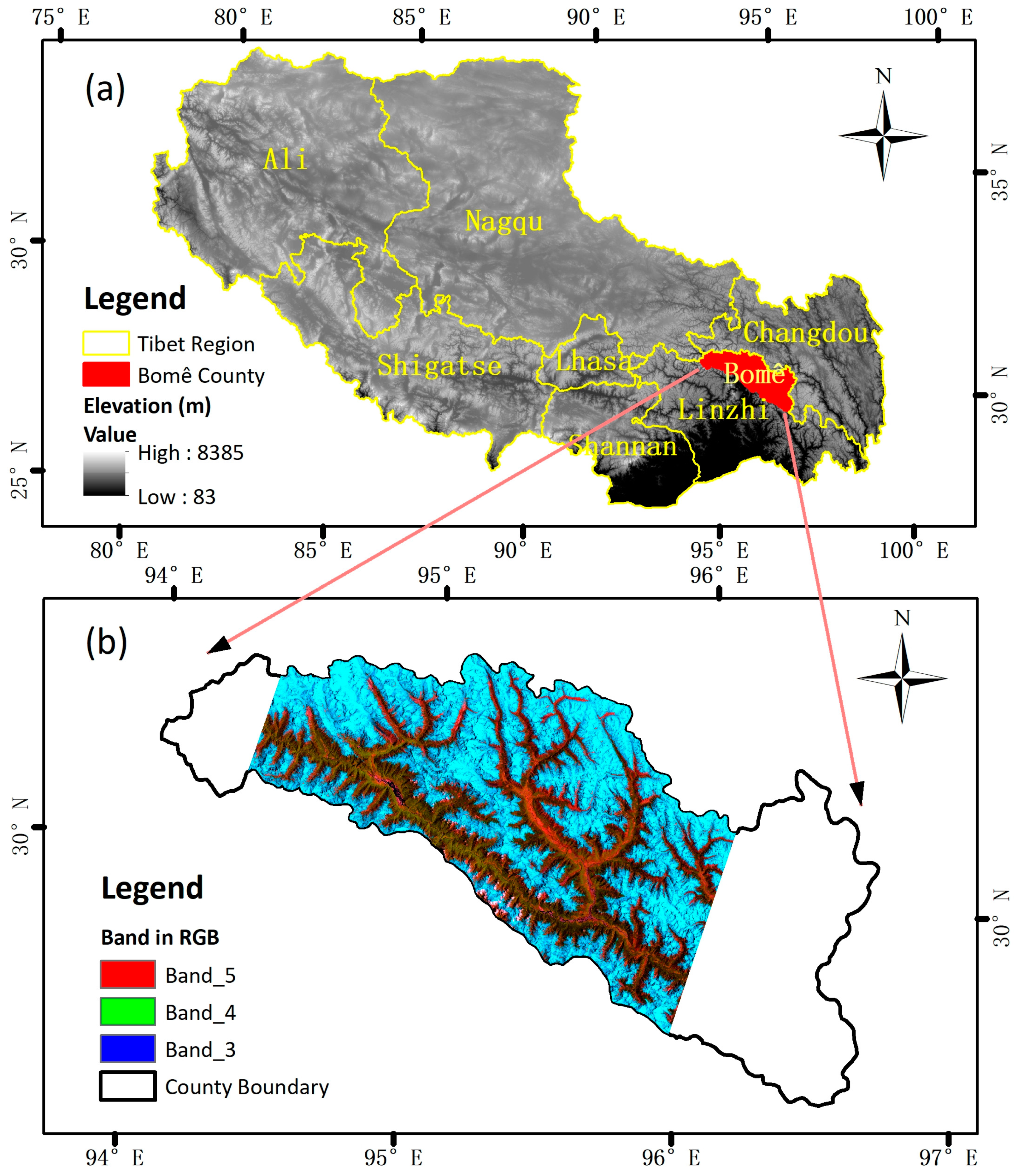
2.1. Study Area

The study area is a part of Bomê County, Tibet, China (Figure 1). Bomê County is located in south-eastern Tibet. Its geographical coordinates are between 29 °N and 30 °N and between 94 °E and 96 °E. It is characterized by a subtropical mountain humid monsoon climate, with an annual mean temperature of 8.5 °C and an annual precipitation of 900 mm. The total land area of Bomê County is 16,795 km2, and the elevation ranges from 2139 m to 6462 m, with a height difference of more than 4000 m. Bomê County is one of the typical representative areas of oceanic glaciers in China and the oceanic glaciers in the area are extremely well developed. Due to its special geographical location and climatic characteristics, glaciers easily accumulate and melt, which increases the difficulty of accurate temporal observations.

2.2. Data and Samples

The study area is fully covered by Landsat path 135 and row 39. Four Landsat image scenes of the different periods (Table 1) were loaded from the Geospatial Data Cloud (http://www.gscloud.cn/) and are all “Tier 1” products, representing the highest quality imagery meeting certain radiometric and geometric requirements.
The four images of the study area, with size 5777 × 4013 pixels, are in the UTM coordinate system geo-referenced to WGS84. We resampled all the image data to a 30 m resolution to ensure that all bands matched the spatial resolution of both the training and validation data. We input all the bands into the classification network for calculation. In addition, the normalized difference vegetation index (NDVI), normalized difference snow index (NDSI), and normalized difference built-up index (NDBI) as input data are also put into the networks to increase the classification accuracy. The NDVI is one of most well-known and frequently used indexes computed from multi-spectral remote sensing [28]. The NDSI is defined as the difference between the reflectances of the green and short-wave infrared bands divided by the sum of the two reflectances [29]. The snow/ice has high reflectance in the visible light region and strong absorption in the SWIR region, which means that the NDSI can effectively distinguish snow from similar bright soils, vegetation and rocks, and clouds in TM images [30]. The NDBI was first proposed in 2003 to extract urban built-up land using Landsat images [31]. The index output ranges from -1 to +1, with positive values representing built-up areas [32]. The NDBI is unable to separate urban areas from bare land, but we can still use it to extract bare land from other land cover types because built-up areas are rare in this region [33]. The NDVI (Equation (1)), NDSI (Equation (2)) and NDBI (Equation (3)) of each image were calculated using the Raster Calculator tool in ArcGIS 10.5:
N D V I = B N B R B N + B R
N D S I = B G B S B G + B S
N D B I = B S B N B S + B N
where BN is the reflectance of the near-infrared band (band 4 for the Landsat 5 TM and Landsat 7 ETM+ sensor and band 5 for the Landsat 8 OLI sensor); BR is the reflectance of the red band (band 3 for Landsat 5 TM/Landsat 7 ETM+ and band 4 for Landsat 8 OLI); BG is the reflectance of the green band (band 2 for Landsat 5 TM/Landsat 7 ETM+ and band 3 Landsat 8 OLI); BS is the reflectance of the short-wave infrared band (band 5 for the Landsat 5 TM and Landsat 7 ETM+ sensor and band 6 for the Landsat 8 OLI sensor).
We used ArcGIS tools to randomly generate 20,000 random points in the study area (the 20,000 sample points on the four images were in the same position). We set the land cover types in this area into vegetation, ice, bare land, clouds, water, and shadows by setting thresholds for NDVI, NDSI, NDBI, and specific spectral bands. The judgment rules are as follows: (1) when a random point is NDVI> = 0.1 and NDVI> NDSI and NDVI> NDBI, it is judged as vegetation; (2) when a random point is NDSI> = 0 and NDSI> NDVI, It is judged as ice or cloud; (3) When a random point has NDBI> = 0.1 and NDBI> NDVI, it is judged as bare ground; (4) When a random point has NDVI <0 and blue band spectral value less than 120 (the blue band spectral value of the OLI sensor is greater than 10,000), it is judged as water; (5) Ice and clouds are distinguished by short-wave infrared. When it is less than 11,000 (for 2016 images only), it is judged as ice; otherwise, it is cloud. Since the other three images selected (1990, 2000 and 2007) were almost cloudless, visual interpretation was used to distinguish between clouds and snow. After the preliminary classification is completed, the four images (1990, 2000, 2007 and 2016) have 280, 567, 341, 1654 points left, respectively, which are inspected by manual judgment based on Google Earth high-resolution images. The number of training/validation points for different land cover types in four years is shown in Table 2, in which three-quarters of each category (75% of the total number of individual categories) were randomly selected as the training set, the remaining (25%) was used as the validation set. The training set and validation set of the CNN are square images of size 7 × 7 pixels with sample points as centre points.

2.3. Methods

The first machine learning algorithm we applied is random forest (RF), which contains multiple decision trees, and every decision tree is trained on different input data sets generated through a bagging procedure, ultimately creating an ensemble of independent experts. The final classification result is based on a collection of all of the trees [34]. To balance the complexity and computational efficiency of the network, the RF algorithm is set to contain 50 decision trees, and the depth of the trees is 5.
The second machine learning algorithm we applied is the BPNN, which consists of forward path and backward path. The forward path involves creating a feed-forward network, initializing the weights, simulation and training the network [17]. The feed-forward network has three parts, namely, input layers, hidden layers and output layers, and at the same time, the layers are directly connected by means of full connections. The backward path is mainly used for updating the network weights and biases that are learned to approximate the complex relationship between the input features and the output characteristics [17]. A specific cost function is used to minimize the difference between the real values and the predicted output [35]. In this study, the BPNN consisted of one hidden layer that had 12 computational nodes. The learning rate and the number of epochs were chosen as 0.01 and 80, respectively. We used a simple and commonly used mean square error loss function.
The third algorithm we used is the CNN algorithm, which was used to process and analyse large-scale sensor data or images by learning stationary characteristics at the local and global scales [23], with alternatively connecting convolutional layers and pooling layers to obtain the deep and abstract features. To balance the complexity and robustness of the network, the CNN was designed to consist of two repetitive parts and three full connected layers. There are two identical convolutional layers and a max pooling layer in each repetitive part, and each convolutional layer is followed by a rectified linear unit activation function. The input size of the CNN is 7 × 7 pixels, the filter size of the convolutional layer was set to 3 × 3 with one stride, and the number of convolutional filters was set to 16, 32, 64, and 128 in turn. The learning rate and batch size were chosen as 0.0001 and 800, respectively. In addition, the number of epochs was set to 200 to learn the features fully with back propagation.
To make full use of spectral information, the input data are the spectral values of all bands and the three indexes (NDVI, NDSI and NDBI). Thus, the input feature numbers of the four years are 10, 12, 10 and 14, respectively. The predicted output of the three networks is expected to be in six classes. Once the final model was trained well; it was applied to an independent set of validation data that was not used to train the models.

2.4. Accuracy Evaluation

We use producer’s accuracy (PA), user’s accuracy (UA), overall accuracy (OA) and Kappa coefficient to evaluate the performance of the three classifiers. The producer’s accuracy and user’s accuracy can be acquired from the confusion matrix. The producer’s accuracy represents the proportion of samples that are correctly classified as category i among all the category i samples (a column of the confusion matrix). The user’s accuracy indicates that among all the samples classified as category i, the measured type is indeed the proportion of category i samples. The overall classification accuracy indicates the proportion of samples that were correctly classified among all the samples. The overall accuracy is proportional to the area that is correctly mapped and is suitable for area estimation. The Kappa coefficient is a measure of the overall agreement in the matrix. In contrast to the overall accuracy, the Kappa coefficient also takes the non-diagonal elements into account and has become a widely used measure of classification accuracy [36]. Since the samples in this study were randomly selected from the entire study area, the classification accuracy can be better evaluated by selecting the above four accuracy evaluation indicators.

2.5. Landscape Indexes

Landscape indexes can effectively summarize the landscape pattern information within a certain range, reflect the structural composition and spatial configuration of different landscape types, and thus quantitatively analyse landscape characteristics and changing trends. The landscape indexes at the class level and landscape level for the four years (1990, 2000, 2007 and 2016) were calculated in Fragstats 4.2 to portray the characteristics of the spatial and temporal changes in the various landscape categories. The class-level indexes reflect the amount and spatial distribution of a single patch type, while the landscape-level indexes reflect the spatial pattern of the entire landscape mosaic [37]. In this study, the class-level indexes, including patch density (PD), mean patch area (AREA_MN), edge density (ED), landscape shape index (LSI), largest patch index (LPI) and aggregation index (AI), were used. In addition to the above indexes, the landscape-level indexes also include the contagion index (CONTAG) and Shannon’s diversity index (SHDI). These indexes are widely used to represent landscape compositions and configurations, as shown in Table 3.
To a certain extent, AREA_MN and the PD both reveal the fragmentation of patches in the landscape elements. AREA_MN reflects the average patch size of the landscape elements. The smaller its value, the higher the fragmentation of the landscape. The PD indicates the fragmentation degree of landscape element patches. The larger the PD value is, the smaller the patch size per unit area and the higher the landscape heterogeneity and fragmentation degree.
The ED is mainly a description of the degree of segmentation of landscape unit composition. The greater the density of the landscape edges is, the greater the degree of landscape fragmentation by the edges. The LSI can describe the regularity and complexity of landscape patch boundaries and refers to the degree of difference between circles or squares with the same patch area and shape. The larger the index value is, the more irregular the shape of the patch, and the less likely it is to be disturbed by the outside world. The LPI quantifies the percentage of the total landscape area composed of the largest patches and is an indicator of the advantages of landscape types. Moreover, the impact of human activities on the landscape can be reflected to some extent by changes in this value. The AI reflects the degree of aggregation. When its value is 0, the degree of fragmentation is the largest. To some extent, it reflects the complexity of the landscape and reveals the degree of human interference in the landscape. CONTAG mainly describes the degree of convergence or extension trend in different patch types in the landscape. In general, a high spread value indicates that a dominant patch type in the landscape has formed good connectivity; otherwise, it indicates that the landscape is more fragmented. The SHDI is the quantifying diversity at the landscape level. When the landscape has only one patch, the SHDI equals 0, and when the patch type increases, the value of the SHDI also increases. The evolution process of landscape patterns can be determined by investigating the basic characteristics, morphological changes and spatiotemporal evolution of the various landscape categories [38].

3. Results

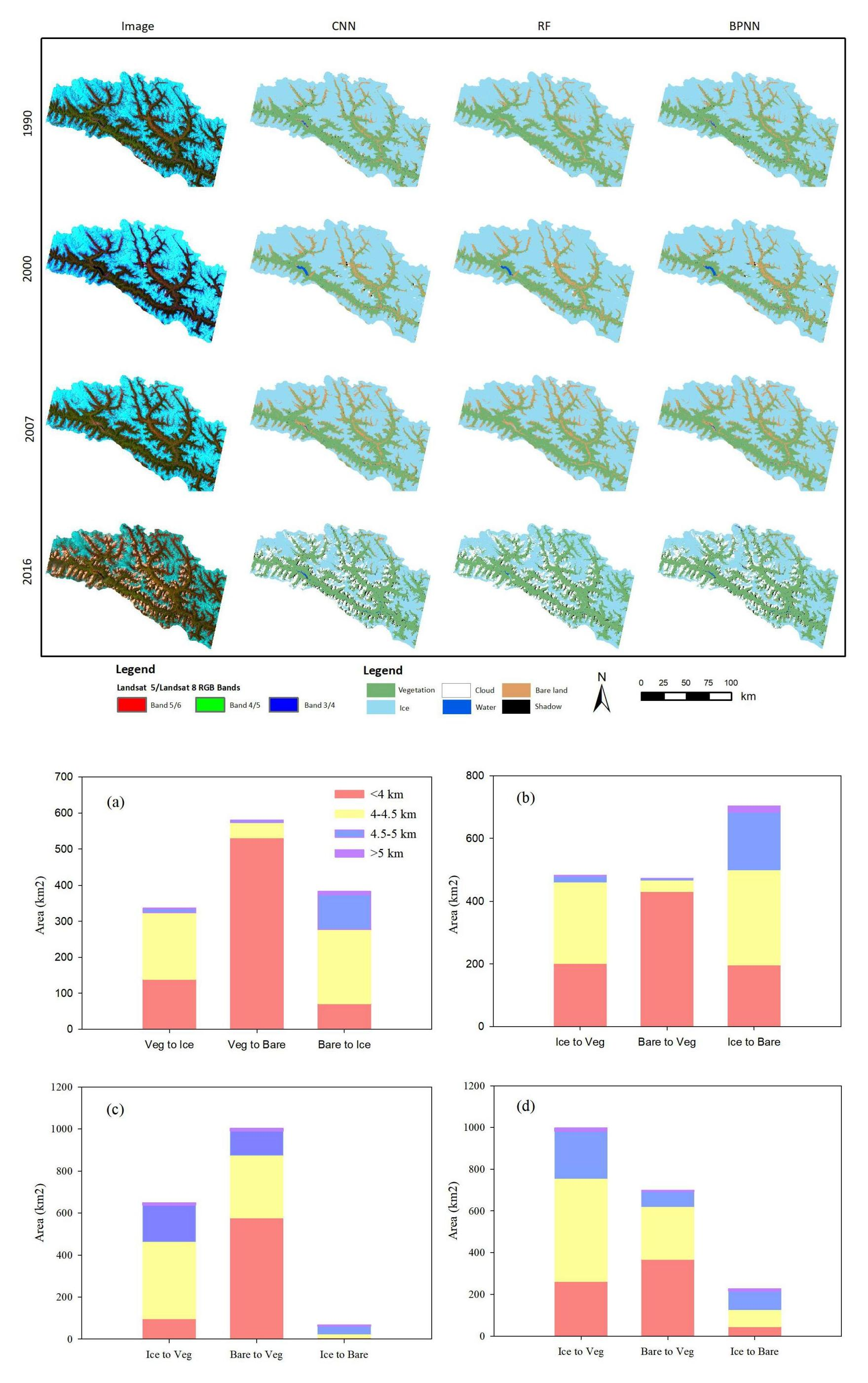
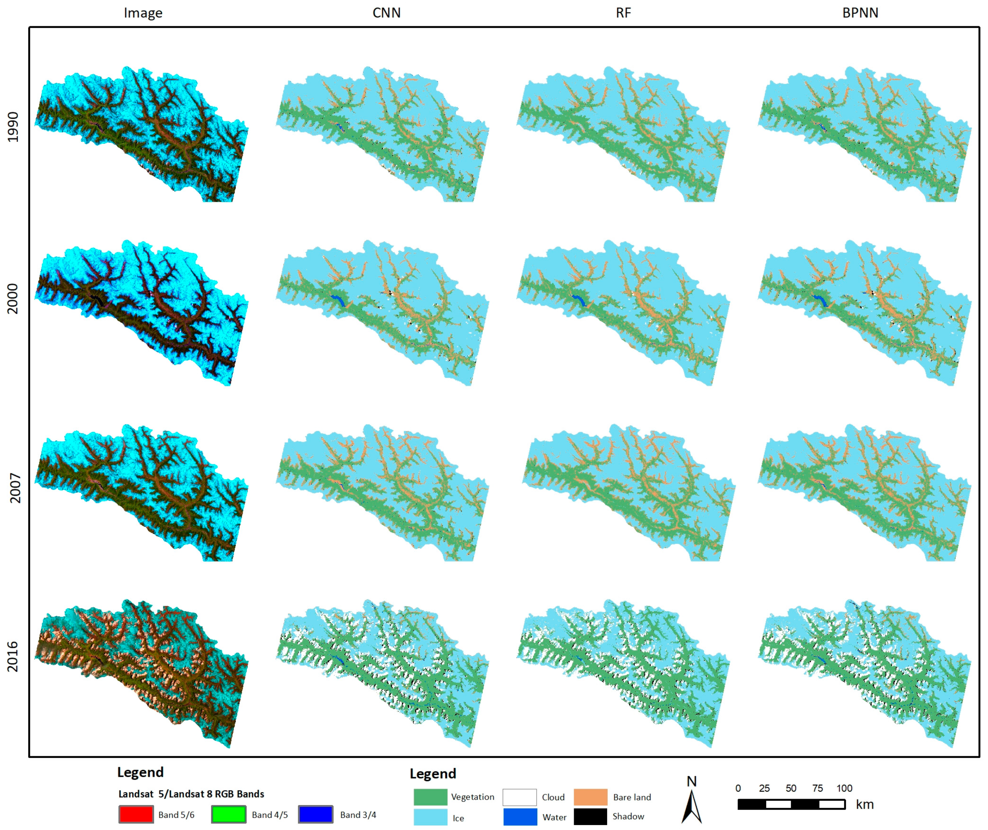
3.1. Classification Accuracy

The classification results are shown in Figure 2. Due to the small number of samples in the categories of water and shadows, only the vegetation, ice, bare land, and clouds are analysed for accuracy here. A summary of the results for three tested models considering four classes is shown (Table 4). Based on Table 4, the BPNN model achieved the highest OAs (97.82%/98.07%/98.92%/94.63%) and Kappa coefficients (0.958/0.959/0.981/0.918) for the four years (1990, 2000, 2007, and 2016, respectively). With the comparison of the RF model (OA 96.46%/97.78%/97.86%/92.55% and Kappa 0.931/0.953/0.962%/0.884%) and the CNN model (OA 95.83%/96.95/96.81%/93.21% and Kappa 0.919/0.935/0.943/0.897), the BPNN improves the OA by more than 1.36%/0.29%/1.06%/2.08% and 1.99%/1.12%/2.11%/1.42%, and the Kappa coefficients by more than 0.027/0.004/0.019/0.034 and 0.039/0.024/0.038/0.021 over the RF model and the CNN model for the four years, respectively. Although the BPNN algorithm is superior to the other two algorithms in terms of the OA and Kappa coefficients, it did not achieve the best accuracy in terms of the PA and UA. For example, for a single kind of vegetation, the UA values of the BPNN algorithm for 1990, 2000, 2007, and 2016 were 97.96%, 97.67%, 99.36%, and 96.60%, respectively, which were higher than those of the RF algorithm (97.73%, 95.07%, 99.04%, and 90.95%, respectively) and that of the CNN algorithm (97.13%, 96.55%, 98.95%, and 96.71%, respectively). For ice, the UA values of the BPNN algorithm on the images at four different periods were 98.65%, 99.44%, 99.48%, and 95.15%, which were 1.01%, 0.06%, 0.59%, and 0.59% higher than the UA values of the RF algorithm, respectively, and were 1.57%, 0.84%, 1.1%, and 1.21% higher than the UA values, respectively, of the CNN algorithm. However, for 2000 and 2016, the PAs of vegetation were 95.75% and 96.45%, which were slightly lower than the RFs of 95.95% and 97.61%, respectively. For ice, the PA value was only 98.67% in 2016, which was higher than the 97.68% PA from the RF model.

3.2. Changes in the Landscape Pattern

To further analyse the landscape pattern characteristics of the land cover types in the study area, we adopted interpolation to remove clouds and shadows. First, the BPNN algorithm classification map with the highest classification accuracy is selected as the base map, and the RF and CNN algorithm classification maps are used as the first and second auxiliary maps, respectively. Second, by overlaying the base map with the first auxiliary map, most of the cloud and shadow areas in the base map are replaced by the land cover types in the RF algorithm classification map, and most of the remaining areas are replaced by the land cover types in the second auxiliary map. Third, the maps from adjacent years are superimposed to remove the remaining cloud and shadow types by temporal replacement. The third step would be performed only if the base map does not completely remove the clouds and shadows after the second step. By interpolating the classification map, the influence of clouds and shadows on the analysis of landscape features is eliminated so that the landscape features of the land cover map can be effectively analysed (Figure 3). Section 3.2.1 and Section 3.2.2 analyse the land cover characteristics of the oceanic glacial regions from the class level and landscape level, respectively.

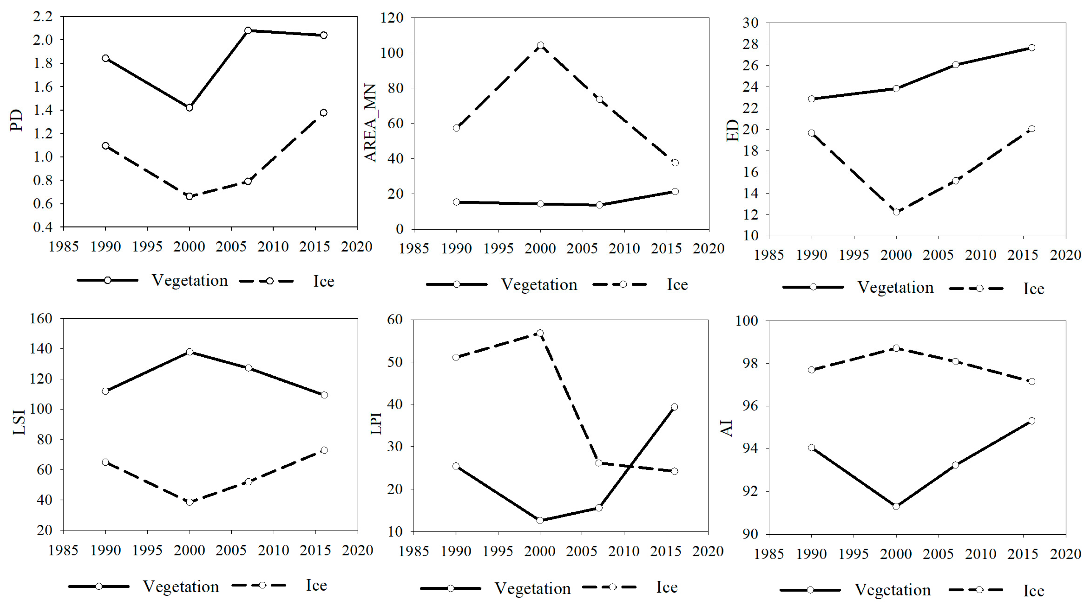
3.2.1. The Class-Level Pattern

The variations in the landscape indexes at the class level from 1990 to 2016 are shown in Figure 4. AREA_MN and the PD both reveal the fragmentation of patches of the landscape elements. The PD value of ice decreased from 1.09 to 0.66 from 1990 to 2000, indicating that the fragmentation of ice was reduced. However, from 2000 to 2016, the fragmentation of ice gradually increased, and the PD value reached 1.38. In contrast, the AREA_MN value of ice increased from 1990 to 2000, while it decreased sharply to 37.66 in 2016. Compared with that in 1990, the AREA_MN value of ice decreased by nearly 20 in 2016. For vegetation, the change trend in the PD value was consistent with that of ice from 1990 to 2000, followed by an increase to 2.08 in 2007. At the same time, the AREA_MN value for vegetation had no obvious change from 1990 to 2005, and it increased slightly from 1990 to 2007. The results show that the fragmentation of ice and vegetation decreased from 1990 to 2000 and increased continuously after 2000.
The ED indicates the complexity of the patch shape, and a low value indicates that the shape is simple. The LSI reflects the irregularity of patch shape and measures the complexity of the spatial pattern of land cover. The ED value of ice decreased dramatically from 19.66 to 12.22 from 1990 to 2000, respectively, while the ED value of ice gradually increased after 2000, reaching 20.04 in 2016, which was roughly the same as that of 1990. The change in the LSI and ED values for ice had the same trend from 1990 to 2016. There was a decreasing trend in the LSI value of ice from 64.79 in 1990 to 38.39 in 2000. After 2000, the LSI value for ice continuously increased and reached the highest peak with a value of 72.70 in 2016. From 1990 to 2016, the ED value of vegetation continued to increase slowly, with an increase of 4.81, indicating that the patch of vegetation became increasingly complex. From 1990 to 2016, the change in the LSI value for vegetation had the opposite trend with that for ice. The LSI for vegetation reached the highest value in 2000, which was 37.79. In addition, the LSI value for vegetation in 2016 was 109.22, which was smaller than the LSI value in 1990. The above results show that compared with other years, the shape of ice in 2000 was more regular and less affected by external disturbances. The edge of the vegetation was the most fragmented, and the fragmentation was large in 2000.
At the landscape class level, the LPI and AI are used here to reflect the degree of aggregation of the landscape elements. The LPI and AI values for ice both increased from 1990, reached the highest peak in 2000, and declined after 2000. In contrast, the LPI and AI values of vegetation both decreased from 1990. They reached the lowest points in 2000 and increased after 2000. Additionally, the AI value for ice was greater than 95 for all four years. Compared with ice, the AI value for vegetation for the four years was lower, but all were greater than 90. Moreover, with respect to the change in the AI values for ice and vegetation, there was an opposite trend. It can be inferred that the degree of ice and vegetation accumulation was high, but the degree of ice accumulation was much higher than that of vegetation. In 2000, the ice had the highest concentration, while the concentration of vegetation was the lowest. From 2000 to 2007, the LPI for ice was much higher than that for vegetation, but the LPI for vegetation exceeded that for ice in 2016. It can be guessed that from 1990 to 2007, ice was the main dominant land cover category in the study area, and in 2016, the vegetation area exceeded that of ice.

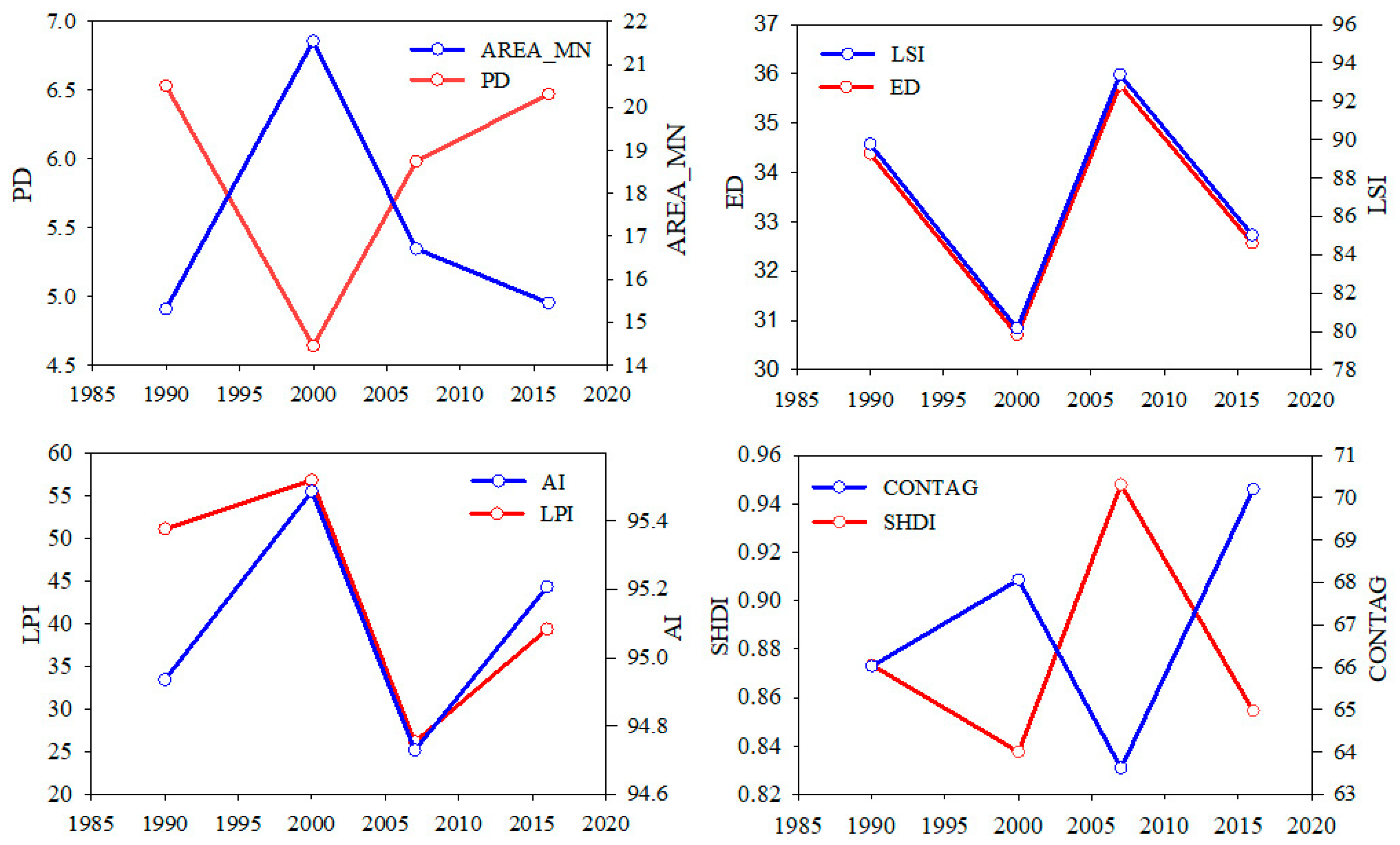
3.2.2. The Landscape-Level Pattern

The AREA_MN and PD can reflect the degree of fragmentation in a landscape. As shown in Figure 5, on the one hand, AREA_MN was approximately 5.0 in 1990, but it rose sharply to 6.8 in 2000 and then dropped to approximately 5.0 in 2016. On the other hand, the PD in 1990 was greater than 6.5, dropped to 4.6 in 2000, and then returned to 6.5 in 2016. In 2000, AREA_MN and the PD reached the highest peak and the lowest valley, respectively, which indicates that landscape fragmentation was large in 2000. From 1990 to 2000, the landscape fragmentation in the study area decreased, and after 2000, the landscape fragmentation increased. The tendency of landscape fragmentation to decrease first and then increase coincides with the trend in the fragmentation of ice and vegetation. It was revealed that the fragmentation of ice and vegetation in the study area reached the minimum in 2000, and the fragmentation increased after 2000. Compared with 1990, the fragmentation did not change much in 2016.
The ED and LSI experienced three stages of changes, and their trends were the opposite at each stage. Their values decreased from 1990 to 2000 and from 2007 to 2016 and increased from 2000 to 2007. The value range of the ED was between 30 and 36, which reflects that the segmentation of the patch edge was not high, and the segmentation change during 1990–2016 was not large. The LSI value varied between 80 and 94, showing that the landscape shape becomes more irregular and complex and that the landscape changed a little due to external disturbance. Therefore, from the changes in the LSI and ED values, we can reveal that compared with other years, the landscape type in this study area was more regular in shape, and the degree of fragmentation was the lowest in 2000. However, compared to 1990, the landscape type in 2016 was slightly simpler and less fragmented.
The LPI values show that the main landscape types increased from 1990 to 2000 and then decreased from 2000 to 2007, consistent with the changes in the LPI for the glaciers from 1990 to 2007, which also shows that ice is the dominant landscape in this period. In addition, the sharply increasing LPI value from 2007 to 2016 is likely to be affected by the type of vegetation because the LPI value for vegetation increased rapidly from 2007 to 2016, and vegetation became the dominant landscape type. From 1990 to 2016, the value of the landscape AI was not less than 94. In addition, according to Figure 4, the AI values for ice from 1990 to 2016 were all greater than 97, and the AI values for vegetation were all greater than 91, with a small fluctuation range. Therefore, according to the above analysis, it can be seen that the concentration of various landscape types in this study area is very high, and the dominant landscape types are ice and vegetation. Moreover, the dominance of ice was higher than that of vegetation from 1990 to 2007, and 2016 was just the opposite.
At the landscape level, the SHDI is calculated mainly because it represents the diversity in the entire landscape level. The SHDI values during 1990–2016 were relatively stable and exhibited a slight overall decrease without significant changes, indicating a slight decrease in landscape diversity. The CONTAG values for the four years in this study area exhibited certain fluctuations, with a maximum value of 70 and a minimum value of 64, indicating that the patch-like connectivity in the study area is good, but the differences vary from year to year. From 1990 to 2000, the value of CONTAG slowly increased to 68, and from 2000 to 2007, the CONTAG value decreased from 68 to 64 and quickly increased to 70 in 2016. The above shows that from 1990 to 2000 and from 2007 to 2016, the connectivity of patches in the study area continued to increase, and the connectivity was the smallest in 2000. In summary, since the dominant patch types in the study area are ice and vegetation, the connectivity for ice and vegetation varies from year to year, and the connectivity is the worst in 2007.

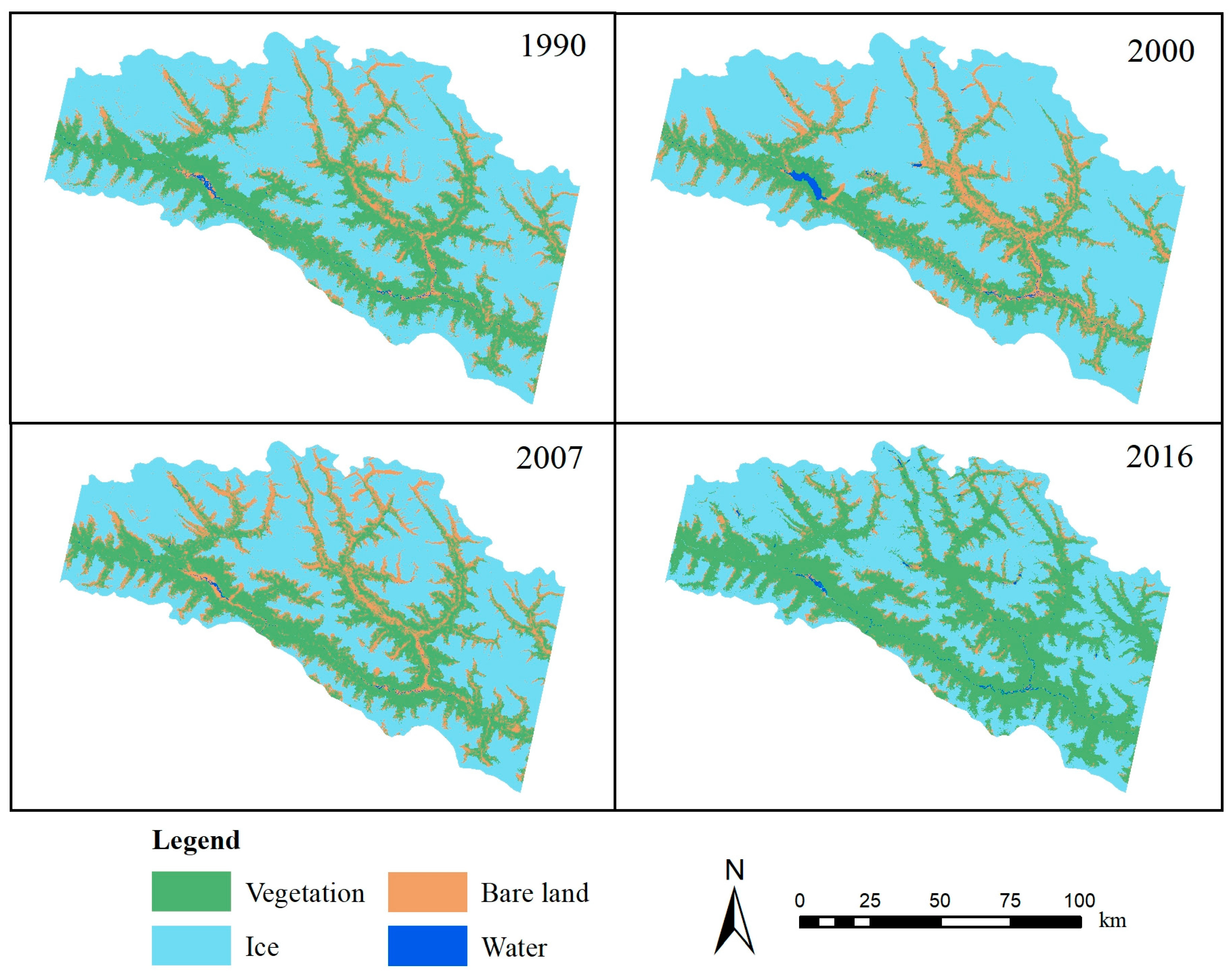
3.3. The Transformation of Land Cover

As shown in Figure 6, the lower semicircle represents the three types of land cover in the previous year, the upper semicircle represents the three types of land cover in the next year, and the transfer between different colors represents the change in the type of land cover (see Figure 6a Veg-1990’s “red” flow to Bare-2000 refers to the percentage of land cover types in 1990 as vegetation, and in 2000 the land cover type became bare land). The land cover structure of the study area greatly changed from 1990 to 2000 (Figure 6a). Among them, the change in ice was the most significant. Approximately 41% of the bare land and 10% of the vegetation were converted into ice, which greatly increased the ice coverage in the area. In addition, nearly 18.7% of the vegetation coverage area was converted into bare land. From 2000 to 2007, the change in ice was relatively small, and nearly half of the area of bare land was converted into vegetation coverage in 2007 (Figure 6b). Figure 6c shows the mutual transfer of land cover types in the study area of Bomê County from 2007 to 2016. We found that most of the bare land has been converted into vegetation, and the glaciers slightly decreased from 2007 to 2016. This finding implies that the glacier area continued to decrease, and the area of vegetation coverage increased significantly from 2000 to 2016. Figure 6d reveals that the land cover structure of Bomê County changed drastically from 1990 to 2016. For instance, nearly three-quarters of the bare land was converted into vegetation. Accordingly, 99.9% of the vegetation areas were unchanged, but the proportion of bare land self-transfer was very low. In summary, our results indicated that vegetation was restored after 2000, and the coverage of vegetation reached its highest amount in 2016.

3.4. Relation between Land Cover Change and Vegetation

To study the mutual conversion relationship between vegetation, ice and bare land at different elevations, the conversion areas from 1990 to 2000, 2000 to 2007, 2007 to 2016, and 1990 to 2016 at different elevation ranges are plotted in Figure 7. Figure 7a shows that from 1990 to 2000, when the elevation was less than 4 km, the area converted from vegetation to ice was almost twice the area converted from bare land to ice. With increasing elevation, the area converted from bare land to ice increases, exceeding the area converted from vegetation to ice. From Figure 7b–d, when the elevation is less than 4 km, the area converted from bare land to vegetation is larger than the area converted from ice to vegetation. However, when the elevation is higher than 4 km, the area converted from ice to vegetation is larger than the area. We can speculate that as elevation increases, vegetation is more likely to convert directly into ice rather than bare land. At the same time, as the elevation increases, the type of land cover converted to vegetation is most likely to be ice rather than bare land. It can be concluded that with increasing elevation, the conversion probability between ice and vegetation is increasing.

4. Discussion

4.1. Comparison of the Classification Algorithms

In this study, three machine learning algorithms were used to classify land cover types in Bomê County, a typical oceanic glacial region. The results show that the BPNN algorithm achieves better classification accuracy than the RF and CNN algorithms. The BPNN is a widely used feed-forward artificial neural network (ANN). By comparing the performances of RF and ANN for the Land use/cover classification, Ge et al. concluded that the highest OA was produced by the ANN (97.16%), which was higher than the RF (96.92%) [40]. Consistent with the classification results, the BPNN used in this study has a higher classification accuracy for the identification of glaciers in oceanic glacial regions. Therefore, the BPNN algorithm has great development potential in oceanic glacial regions. Yoo et al. made a detailed comparison between CNN and RF classifiers to find that CNN consistently resulted in higher accuracy than RF, and OA increased by 7%–18% [41]. However, the OA for the CNN algorithm is inferior to those of the BPNN and RF in this study. In the CNN-based scheme, the influence of neighbourhood pixels as input features is considered. However, a common practical problem based on deep learning classifiers is the class imbalance problem, which means that some neighbourhood classes have more examples in the training set than others. The overall accuracy measure is related to difficulties in the context of imbalanced data, and class imbalances can have an adverse effect on the training of deep learning classifiers [42]. This problem affects both the convergence of the training phase and the generalization ability of the model on the test set. In this study, due to the different neighbourhood sample sizes of the six categories, there is a certain class imbalance in the training and test samples in CNN compared with that in BPNN and RF, which may mislead the class label of training set and affect the CNN classification performance.
Although the three algorithm models have shown good performance in the classification of land cover changes in oceanic glaciers regions, the three algorithm models have different degrees of misclassification. The RF model incorrectly classifies “bare land” as “vegetation” and “vegetation” as “bare land”, resulting in the phenomenon of unclear boundary between these classes of bare land and vegetation. Confusion between “vegetation” and “bare land” is also present in the CNN results, but it is not as strong as for the RF method. Both BPNN model and CNN model reduces the confusion between “ice” and “cloud” as well as “ice” and “shadow” compared to the RF method and improve the accuracy of these categories, but BPNN model still shows a tendency to misclassify “water”. The artificial definition of thresholds between land cover categories for training samples may reduce the accuracy of land cover classification in oceanic glacial regions and thus, affects the analysis of land cover changes to a certain extent.

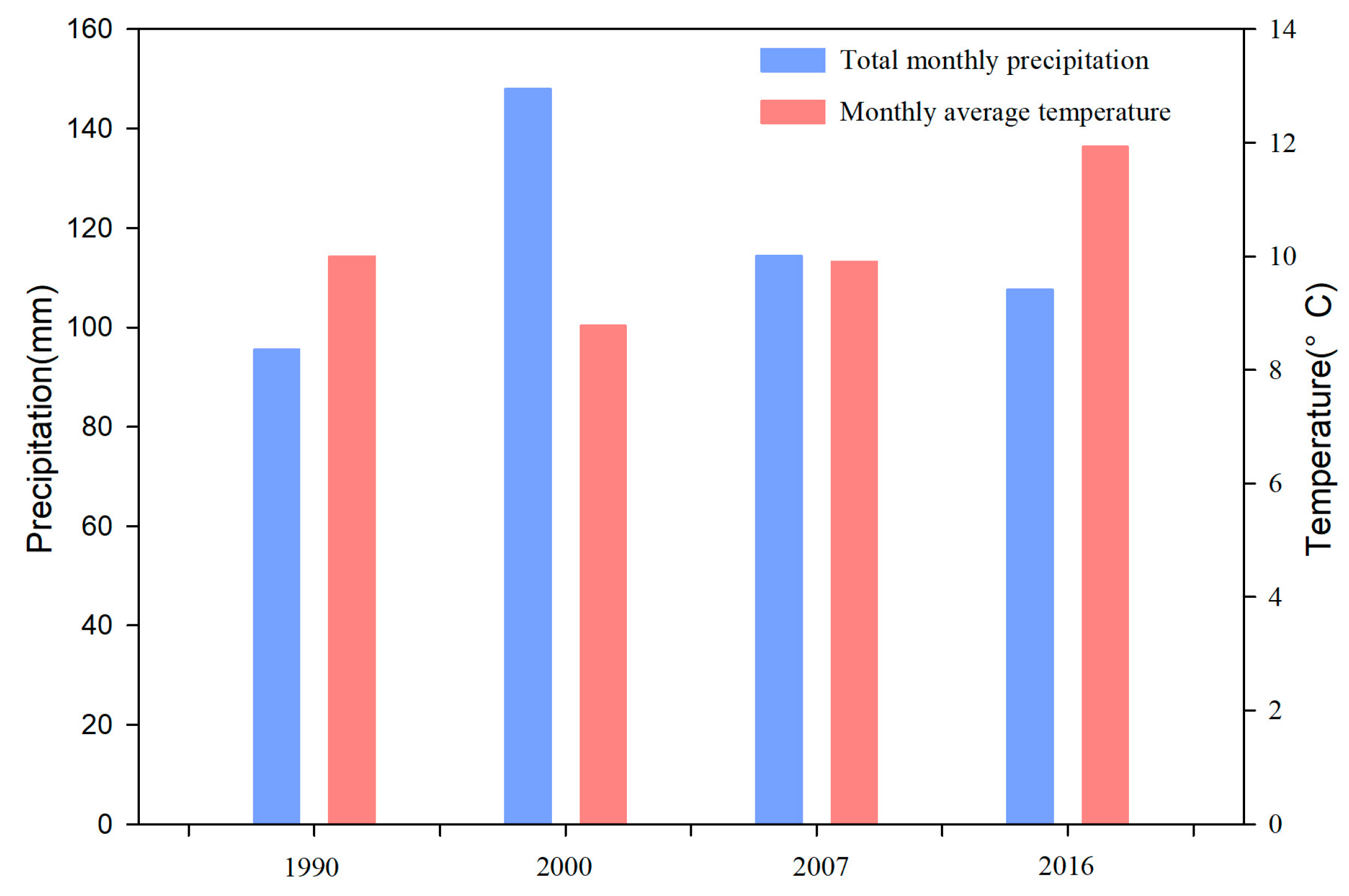
4.2. Driving Forces for Land Cover Change

Of the types of glaciers, oceanic glaciers are most sensitive to changes in temperature and precipitation, especially temperature changes [43]. An increase in temperature will cause glaciers to melt, and an increase in precipitation will increase the accumulation of glaciers. However, the increase in glaciers caused by the increase in annual precipitation is not enough to offset the increased ablation due to rising temperatures [44]. To understand the reasons for the changes in glaciers and vegetation, we downloaded the precipitation and temperature data of Bomê County from 1990, 2000, 2007 and 2016 from the China Meteorological Data Network (http://data.cma.cn/site/index.html) and calculated the total precipitation and average temperature one month before the image acquisition time in the study area (one month means 30 days), as shown in Figure 8. The precipitation in the study area showed a rapid increase from 1990 to 2000, with 95.6 mm of the monthly precipitation in 1990, increasing significantly to 148.0 mm in 2000. The monthly average temperature in the study area decreased from 10 degrees in 1990 to 8.78 degrees in 2000. Many studies have shown that an increase in temperature will cause glaciers to melt, and an increase in precipitation will increase the accumulation of glaciers [1,43]. Even if the temperature changes slightly, the glaciers may experience dramatic changes [11]. Consistently with the results of these scholars, the decrease in the average monthly temperature and the significant increase in the monthly precipitation can explain the dramatic increase in ice and decrease in the area coverage by vegetation from 1990 to 2000. After 2000, the average monthly temperature in the study area continued to increase at the same rate, reaching 9.91 degrees in 2007 and 11.93 degrees in 2016. For nearly three decades from 1990 to 2016, the average monthly temperature in the study area increased by approximately 2 degrees. In addition, the monthly average precipitation in the study area began to decrease, reaching 107.6 mm in 2016, but still higher than the original 95.6 mm in 1990. Chen et al. studied that the increase in glaciers caused by the increase in annual precipitation is not enough to offset the increased ablation due to rising temperatures [44]. Consistently with his results, glaciers decreased from 1990 to 2016 because the increase in glaciers caused by increased rainfall was less than that caused by temperature increases and confirmed temperature rise is the dominant factor in the rapid retreat of glaciers in this area [45]. From Figure 6d, the vegetation age began to gradually recover, and ice melted after 2000. The continuous decrease in precipitation and the relative increase in temperature can be attributed to this phenomenon.

4.3. Shortcomings and Prospects

Because glaciers in the southeast of Tibet are relatively least and the growth of vegetation can be effectively monitored in the summer, we generally prefer images acquired in summer to monitor land cover changes in southeast Tibet. However, due to the cloudy weather in summer, it is very difficult to obtain cloudless or low-cloud images in the summer in this area. Therefore, we selected four near-summer images from Bomê County (May 17, 1990, May 4, 2000, April 30, 2007, and May 24, 2016). Not only do they maintain a certain time span one year, but the time of image acquisition is spanning in one month. In future research, image fusion technology can be used to remove the cloud from the image to obtain a long-term continuous sequence of images to further analyze the land cover changes in the southeastern Tibet. Moreover, this study used Landsat images with a resolution of 30 m and a revisit period of 16 days. Due to the high cloud cover rate in the study area, Landsat images that can meet the cloud cover rate requirements are very limited, which results in coarse resolution. In future land cover classification in oceanic glacial regions, satellite data with high spatiotemporal resolution will obtain more information and perform more detailed analysis after data fusion. In addition, in terms of algorithms, although the CNN do not obtain the best classification results, in the field of deep learning, combining a CNN and other machine learning methods for land cover change analysis in oceanic glacial regions is also a very promising research direction [46].

5. Conclusions

The glaciers in southeast Tibet are the largest monsoon-type oceanic glaciers in China. As the temperature rises, the glaciers gradually melt, and the land cover in the glacial area also changes greatly, which has a significant impact on the stability of the ecosystem in Tibet. This study uses Landsat satellite images and three machine learning algorithms, namely, the RF, BPNN and CNN algorithms, to classify land cover in Bomê County. Three findings from the observations and algorithms are provided as follows.
First, the dominant land cover type was converted from ice to vegetation, and the landscape aggregation of ice decreased, indicating the influence of global warming. Second, in addition to the greatest transformation between vegetation and bare land, the probability of direct transformation between vegetation and ice increased when the elevation was higher than 4 km. Finally, although the RF and CNN algorithms have been widely applied in remote sensing image classification, this study shows the effectiveness of the BPNN algorithm in image classification for typical regions. Because clouds and mountain shadows influence the temporal and spatial quality of Landsat images for oceanic glacier mapping in Tibet, satellite data with high spatiotemporal resolutions are required in future studies, which should depend on the exploration of suitable data fusion algorithms.

Author Contributions

Conceptualization, Y.L.; methodology, F.Y. and Y.L.; software, F.Y. and K.L.; validation, F.Y.; formal analysis, F.Y.; data curation, F.Y. and P.H.; writing—original draft preparation, F.Y.; writing—review and editing, J.C. and Y.L; supervision, Y.L. and L.X. All authors have read and agreed to the published version of the manuscript.

Funding

This research is financially supported by the Second Tibetan Plateau Scientific Expedition and Research Program (2019QZKK0405); the Strategic Priority Research Program of Chinese Academy of Sciences (XDA20020402); and the National Natural Science Foundation of China (41861134038).

Conflicts of Interest

The authors declare no conflicts of interest.

References

  1. Yao, T.; Thompson, L.; Yang, W.; Yu, W.; Gao, Y.; Guo, X.; Yang, X.; Duan, K.; Zhao, H.; Xu, B.; et al. Different glacier status with atmospheric circulations in Tibetan Plateau and surroundings. Nat. Clim. Chang. 2012, 2, 663–667. [Google Scholar] [CrossRef]
  2. Pan, C.G.; Pope, A.; Kamp, U.; Dashtseren, A.; Walther, M.; Syromyatina, M.V. Glacier recession in the Altai Mountains of Mongolia in 1990–2016. Geogr. Ann. Ser. Phys. Geogr. 2018, 100, 185–203. [Google Scholar] [CrossRef]
  3. Barry, R.G. The status of research on glaciers and global glacier recession: A review. Prog. Phys. Geogr. Earth Environ. 2006, 30, 285–306. [Google Scholar] [CrossRef]
  4. Mu, J.; Li, Z.; Zhang, H.; Liang, P. The global glacierized area: Current situation and recent change, based on the Randolph Glacier Inventory (RGI 6.0) published in 2017. J. Glaciol. Geocryol. 2018, 40, 238–248. [Google Scholar]
  5. Pritchard, H.D. Asia’s shrinking glaciers protect large populations from drought stress. Nature 2019, 569, 649–654. [Google Scholar] [CrossRef]
  6. Immerzeel, W.W.; Lutz, A.F.; Andrade, M.; Bahl, A.; Biemans, H.; Bolch, T.; Hyde, S.; Brumby, S.; Davies, B.J.; Elmore, A.C.; et al. Importance and vulnerability of the world’s water towers. Nature 2020, 577, 364–369. [Google Scholar] [CrossRef]
  7. Wilson, R.; Harrison, S.; Reynolds, J.; Hubbard, A.; Glasser, N.F.; Wundrich, O.; Anacona, P.I.; Mao, L.; Shannon, S. The 2015 Chileno Valley glacial lake outburst flood, Patagonia. Geomorphology 2019, 332, 51–65. [Google Scholar] [CrossRef]
  8. Bajracharya, S.R.; Mool, P. Glaciers, glacial lakes and glacial lake outburst floods in the Mount Everest region, Nepal. Ann. Glaciol. 2009, 50, 81–86. [Google Scholar] [CrossRef] [Green Version]
  9. Shi, Y.F.; Liu, S.Y. Estimation on the response of glaciers in China to the global warming in the 21st century. Chin. Sci. Bull. 2000, 45, 668–672. [Google Scholar] [CrossRef]
  10. Su, Z.; Shi, Y.F. Response of monsoonal temperate glaciers to global warming since the Little Ice Age. Quat. Int. 2002, 97–98, 123–131. [Google Scholar] [CrossRef]
  11. Yang, W.; Yao, T.; Xu, B.; Ma, L.; Wang, Z.; Wan, M. Characteristics of recent temperate glacier fluctuations in the Parlung Zangbo River basin, southeast Tibetan Plateau. Chin. Sci. Bull. 2010, 55, 2097–2102. [Google Scholar] [CrossRef]
  12. Gong, J.; Li, J.; Yang, J.; Li, S.; Tang, W. Land use and land cover change in the Qinghai lake region of the Tibetan Plateau and its impact on ecosystem services. Int. J. Environ. Res. Public Health 2017, 14, 818. [Google Scholar] [CrossRef] [PubMed]
  13. Chen, D. Assessment of past, present and future environmental changes on the Tibetan Plateau. Chin. Sci. Bull. 2015, 60, 3025–3035, (In Chinese with English abstract). [Google Scholar]
  14. Cui, X.; Graf, H.-F. Recent land cover changes on the Tibetan Plateau: A review. Clim. Chang. 2009, 94, 47–61. [Google Scholar] [CrossRef] [Green Version]
  15. Song, W.; Deng, X. Land-use/land-cover change and ecosystem service provision in China. Sci. Total Environ. 2017, 576, 705–719. [Google Scholar] [CrossRef]
  16. Xu, X.; Chen, H.; Levy, J.K. Spatiotemporal vegetation cover variations in the Qinghai-Tibet Plateau under global climate change. Sci. Bull. 2008, 53, 915–922. [Google Scholar] [CrossRef] [Green Version]
  17. Le Bris, R.; Paul, F.; Frey, H.; Bolch, T. A new satellite-derived glacier inventory for western Alaska. Ann. Glaciol. 2011, 52, 135–143. [Google Scholar] [CrossRef] [Green Version]
  18. Duan, C.; Shi, P.; Song, M.; Zhang, X.; Zong, N.; Zhou, C. Land use and land cover change in the Kailash sacred landscape of China. Sustainability 2019, 11, 1788. [Google Scholar] [CrossRef] [Green Version]
  19. Song, X.; Yang, G.; Yan, C.Z.; Hanchen, D.; Liu, G.; Zhu, Y. Driving forces behind land use and cover change in the Qinghai-Tibetan Plateau: A case study of the source region of the Yellow River, Qinghai Province, China. Environ. Earth Sci. 2009, 59, 793–801. [Google Scholar] [CrossRef]
  20. Li, Z.; Tian, L.; Wu, H.; Wang, W.; Zhang, S.; Zhang, J.; Li, X. Changes in glacier extent and surface elevations in the Depuchangdake region of northwestern Tibet, China. Quat. Res. 2016, 85, 25–33. [Google Scholar] [CrossRef]
  21. Duan, H.; Yao, X.; Liu, S.; Gao, Y.; Qi, M.; Liu, J.; Zhang, D.; Li, X. Glacier change in the Tanggula Mountains, Tibetan Plateau, in 1969–2015. J. Mt. Sci. 2019, 16, 2663–2678. [Google Scholar] [CrossRef]
  22. Wang, L.; Lu, A.; Yao, T.; Wang, N. The study of typical glaciers and lakes fluctuations using remote sensing in Qinghai-Tibetan Plateau. In Proceedings of the 2007 IEEE International Geoscience and Remote Sensing Symposium, Barcelona, Spain, 23–27 July 2007. [Google Scholar]
  23. LeCun, Y.; Bengio, Y.; Hinton, G. Deep learning. Nature 2015, 521, 436–444. [Google Scholar] [CrossRef] [PubMed]
  24. Gislason, P.O.; Benediktsson, J.A.; Sveinsson, J.R. Random forests for land cover classification. Pattern Recognit. Lett. 2006, 27, 294–300. [Google Scholar] [CrossRef]
  25. Buscema, M. Back propagation neural networks. Subst. Use Misuse 1998, 33, 233–270. [Google Scholar] [CrossRef]
  26. Li, S.; Song, W.; Fang, L.; Chen, Y.; Ghamisi, P.; Benediktsson, J.A. Deep learning for hyperspectral image classification: An overview. IEEE Trans. Geosci. Remote Sens. 2019, 57, 6690–6709. [Google Scholar] [CrossRef] [Green Version]
  27. Wei, Y.; Wang, S.; Liu, J.; Zhou, L. Multi-source remote-sensing monitoring of the monsoonal maritime glaciers at Mt. Dagu, East Qinghai-Tibetan Plateau, China. IEEE Access 2019, 7, 48307–48317. [Google Scholar] [CrossRef]
  28. Potter, C.; Li, S.; Huang, S.; Crabtree, R.L. Analysis of sapling density regeneration in Yellowstone National Park with hyperspectral remote sensing data. Remote Sens. Environ. 2012, 121, 61–68. [Google Scholar] [CrossRef]
  29. Keshri, A.K.; Shukla, A.; Gupta, R.P. ASTER ratio indices for supraglacial terrain mapping. Int. J. Remote Sens. 2008, 30, 519–524. [Google Scholar] [CrossRef]
  30. Hall, D.K.; Riggs, G.A.; Salomonson, V.V. Development of methods for mapping global snow cover using moderate resolution imaging spectroradiometer data. Remote Sens. Environ. 1995, 54, 127–140. [Google Scholar] [CrossRef]
  31. Zha, Y.; Gao, J.; Ni, S. Use of normalized difference built-up index in automatically mapping urban areas from TM imagery. Int. J. Remote Sens. 2003, 24, 583–594. [Google Scholar] [CrossRef]
  32. Mathivanan, M. Monitoring spatio-temporal dynamics of urban and peri-urban land transitions using ensemble of remote sensing spectral indices—A case study of Chennai Metropolitan Area, India. Environ. Monit. Assess. 2019, 192, 15. [Google Scholar] [CrossRef]
  33. He, C.; Shi, P.; Xie, D.; Zhao, Y. Improving the normalized difference built-up index to map urban built-up areas using a semiautomatic segmentation approach. Remote Sens. Lett. 2010, 1, 213–221. [Google Scholar] [CrossRef] [Green Version]
  34. Breiman, L. Random forests. Mach. Learn. 2001, 45, 5–32. [Google Scholar] [CrossRef] [Green Version]
  35. Strigl, D.; Kofler, K.; Podlipnig, S. Performance and scalability of GPU-based convolutional neural networks. In Proceedings of the 2010 18th Euromicro Conference on Parallel, Distributed and Network-based Processing, Pisa, Italy, 17–19 Feburay 2010; pp. 317–324. [Google Scholar]
  36. Congalton, R.G. A review of assessing the accuracy of classifications of remotely sensed data. Remote Sens. Environ. 1991, 37, 35–46. [Google Scholar] [CrossRef]
  37. McGarigal, K.S.; Cushman, S.; Neel, M.; Ene, E. FRAGSTATS: Spatial Pattern Analysis Program for Categorical Maps. Available online: https://www.umass.edu/landeco/research/fragstats/downloads/fragstats_downloads.html (accessed on 19 March 2020).
  38. Zhu, Y.; Wang, C.; Takeru, S. Remote sensing-based analysis of landscape pattern evolution in industrial rural areas: A case of Southern Jiangsu, China. Sustainability 2019, 11, 4994. [Google Scholar] [CrossRef] [Green Version]
  39. O’Neill, R.V.; Krummel, J.R.; Gardner, R.H.; Sugihara, G.; Jackson, B.; DeAngelis, D.L.; Milne, B.T.; Turner, M.G.; Zygmunt, B.; Christensen, S.W.; et al. Indices of landscape pattern. Landsc. Ecol. 1988, 1, 153–162. [Google Scholar] [CrossRef]
  40. Ge, G.; Shi, Z.; Zhu, Y.; Yang, X.; Hao, Y. Land use/cover classification in an arid desert-oasis mosaic landscape of China using remote sensed imagery: Performance assessment of four machine learning algorithms. Glob. Ecol. Conserv. 2020, 22, e00971. [Google Scholar] [CrossRef]
  41. Yoo, C.; Han, D.; Im, J.; Bechtel, B. Comparison between convolutional neural networks and random forest for local climate zone classification in mega urban areas using Landsat images. ISPRS J. Photogramm. Remote Sens. 2019, 157, 155–170. [Google Scholar] [CrossRef]
  42. Buda, M.; Maki, A.; Mazurowski, M.A. A systematic study of the class imbalance problem in convolutional neural networks. Neural Netw. 2018, 106, 249–259. [Google Scholar] [CrossRef] [Green Version]
  43. Fujita, K. Effect of precipitation seasonality on climatic sensitivity of glacier mass balance. Earth Planet. Sci. Lett. 2008, 276, 14–19. [Google Scholar] [CrossRef]
  44. Chen, H.; Yang, J.; Tan, C. Responsivity of glacier to climate change in China. J. Glaciol. Geocryol. 2017, 39, 16–23. [Google Scholar]
  45. Xiang, L.; Liu, Z.; Liu, J. Variation of glaciers and its response to climate change in Bomi County of Tibet autonomous region in 1980–2010. J. Glaciol. Geocryol. 2013, 35, 593–600. [Google Scholar]
  46. Zhang, C.; Pan, X.; Li, H.; Gardiner, A.; Sargent, I.; Hare, J.; Atkinson, P.M. A hybrid MLP-CNN classifier for very fine resolution remotely sensed image classification. ISPRS J. Photogramm. Remote Sens. 2018, 140, 133–144. [Google Scholar] [CrossRef] [Green Version]
Figure 1. Study area: (a) Tibet, China; (b) Study area. Standard false colour composite image from Landsat-5, 17 May 1990.
Remotesensing 12 00999 g001
Figure 2. Classification results of the three methods. The first column represents the original image, and the second to fourth columns are the classification results of the three different algorithms: CNN, RF, and BPNN. Each row represents a fixed year; from top to bottom: 1990, 2000, 2007, and 2016.
Remotesensing 12 00999 g002
Figure 3. Cloudless land cover maps for the four years: 1990, 2000, 2007 and 2016.
Remotesensing 12 00999 g003
Figure 4. Changes in the class-level landscape indexes (PD, AREA_MN, ED, LSI, LPI, and AI) from 1990-2016.
Remotesensing 12 00999 g004
Figure 5. Changes in the landscape-level landscape indexes (PD, AREA_MN, ED, LSI, LPI, AI, SHDI, and CONTAG) from 1990-2016.
Remotesensing 12 00999 g005
Figure 6. Landscape type transition matrix in the study area. (ad) show the changes from 1990 to 2000, 2000 to 2007, 2007 to 2016, and 1990 to 2016. A-B refers to land cover type A in year B. e.g., Veg-1990 indicates that the type of land cover in 1990 was vegetation.
Remotesensing 12 00999 g006
Figure 7. Area conversion diagram of the land cover types (vegetation, ice, and bare land) at different elevations in different years. (a) 1990 to 2000; (b) 2000 to 2007; (c) 2007 to 2016; (d) 2007 to 2016. Besides, “Veg” means vegetation, “Bare” means bare land, and “Ice” means ice.
Remotesensing 12 00999 g007
Figure 8. Total monthly precipitation and monthly average temperature in the study area in 1990, 2000, 2007 and 2016.
Remotesensing 12 00999 g008
Table 1. Acquired satellite images of study area.
ImageSatelliteAcquisition DateCloud Coverage
Image 1Landsat 51990-05-173%
Image 2Landsat 72000-05-041.23%
Image 3Landsat 52007-04-301.75%
Image 4Landsat 82016-05-2415%
Table 2. Number of training and verification points for six land cover types in 1990, 2000, 2007 and 2016 (“T” for training points and “V” for validation points).
1990200020072016
TVTVTVTV
Vegetation4097136528949654216140556571885
Ice921830731019833998588286260902030
Bare land11883961431477186862223578
Cloud371263211032235745
Water5317862833118428
Shadow1615482274013453151
Table 3. Landscape pattern indexes used in this study.
NameCalculation FormulaNotes
Patch Density (PD) [39] P D = N A ( 10 , 000 ) ( 100 ) N = the total number of patches
A = total landscape area (m2).
Mean Patch Area
(AREA_MN) [37]
A R E A _ M N = A N A = total landscape area (m2).
N = the total number of patches.
Edge Density (ED) [37] E D = E A ( 10 , 000 ) E = total length (m) of edge in landscape.
A = total landscape area (m2).
Landscape Shape Index (LSI) [37] L S I = 0.25 E * A E* = total length (m) of the landscape edge; includes the entire landscape boundary and some or all background edge segments.
A = total landscape area (m2).
Largest Patch Index (LPI) [39] L P I = max ( a i j ) A ( 100 ) aij = the area (m2) of patches numbered ij.
A = total landscape area (m2).
Aggregation Index (AI) [37] A I = [ i = 1 m ( g i i max g i i ) P i ] ( 100 ) gii = number of like adjacencies (joins) between pixels of patch type (class) i based on the single-count method.
Max->gii = maximum number of like adjacencies (joins) between pixels of patch type (class) i (see below) based on the single-count method.
Pi = proportion of landscape comprised of patch type (class) i.
Contagion Index (CONTAG) [39] C O N T A G = [ 1 + i = 1 m k = 1 m [ ( P i g i k k = 1 m g i k ) ] [ ln ( P i g i k k = 1 m g i k ) ] 2 l n ( m ) ] ( 100 ) Pi = proportion of the landscape occupied by patch type (class) i.
gik = number of adjacencies (joins) between pixels of patch types (classes) i and k based on the double-count method.
m = number of patch types (classes) present in the landscape, including the landscape border if present.
Shannon’s Diversity Index (SHDI) [39] S H D I = i = 1 m P i ln ( P i ) Pi = proportion of landscape comprised of patch type (class) i.
Table 4. Classification accuracy of the RF, CNN and BPNN model.
ClassVegetationIceBare LandCloud
UA(%)PA(%)UA(%)PA(%)UA(%)PA(%)UA(%)PA(%)OA(%)Kappa
1990RF97.7394.6597.6499.8784.3994.1983.3341.6796.460.931
CNN97.1394.3697.0899.5893.7184.3410075.0095.910.921
BPNN97.9698.3298.6599.7791.8393.6983.3383.3397.820.958
2000RF95.0795.9599.3899.7692.0096.44066.6797.780.953
CNN96.5592.9598.6099.6887.3591.1985.7185.7196.990.936
BPNN97.6795.7599.4499.6290.8595.8178.9571.4398.070.959
2007RF99.0495.6698.8999.9091.0297.750097.860.962
CNN98.9594.2398.3899.6288.6994.530097.070.948
BPNN99.3699.2999.4899.7695.9097.750098.920.981
2016RF90.9597.6194.9397.680090.1987.6592.550.884
CNN96.7191.9493.9498.4744.8383.3395.0289.6693.190.897
BPNN96.6096.4595.1598.6769.4496.1592.6387.7994.630.918

