Extracting Agronomic Information from SMOS Vegetation Optical Depth in the US Corn Belt Using a Nonlinear Hierarchical Model

Abstract

Remote sensing observations that vary in response to plant growth and senescence can be used to monitor crop development within and across growing seasons. Identifying when crops reach specific growth stages can improve harvest yield prediction and quantify climate change. Using the Level 2 vegetation optical depth (VOD) product from the European Space Agency’s Soil Moisture and Ocean Salinity (SMOS) satellite, we retrospectively estimate the timing of a key crop development stage in the United States Corn Belt. We employ nonlinear curves nested within a hierarchical modeling framework to extract the timing of the third reproductive development stage of corn (R3) as well as other new agronomic signals from SMOS VOD. We compare our estimates of the timing of R3 to United States Department of Agriculture (USDA) survey data for the years 2011, 2012, and 2013. We find that 87%, 70%, and 37%, respectively, of our model estimates of R3 timing agree with USDA district-level observations. We postulate that since the satellite estimates can be directly linked to a physiological state (the maximum amount of plant water, or water contained within plant tissue per ground area) it is more accurate than the USDA data which is based upon visual observations from roadways. Consequently, SMOS VOD could be used to replace, at a finer resolution than the district-level USDA reports, the R3 data that has not been reported by the USDA since 2013. We hypothesize the other model parameters contain new information about soil and crop management and crop productivity that are not routinely collected by any federal or state agency in the Corn Belt.

1. Introduction

The United States Department of Agriculture (USDA) National Agricultural Statistics Service (NASS) produces weekly growing-season Crop Progress and Condition reports. Crop progress data includes information such as the percentage of different crops that have been planted, the percentage that have reached specific development stages, and the percentage harvested. The data are collected by “enumerators” or human volunteers who make visual observations from roadways. Despite inherent inaccuracies, these reports are particularly important in the United States Corn Belt, a large region of corn and soybean production covering more than 10 different states and worth more than $100 billion annually, because they influence marketing decisions as measured by variance in close-to-open crop trading values and changes in market prices when new crop progress information becomes available [1]. Consequently, many efforts have been made to use remotely sensed observations to automate monitoring of crop progress with the ultimate goal of predicting crop yield.

There are three main bands of electromagnetic radiation that have been found to be related to crop progress [2] and/or crop yield [3]. The visible and near-infrared (optical) reflectance of a crop canopy changes with leaf properties. Leaves take in the carbon used in photosynthesis to create plant matter. Solar-induced fluorescence is also sensitive to photosynthesis. The infrared radiation emitted by vegetation is a function of its temperature, which can be used to infer evapotranspiration (ET) and hence crop stress that can either accelerate or retard development and reduce yield. Finally, both microwave backscatter and emission can also be used to observe vegetation. The vegetation optical depth (VOD) retrieved from observed brightness temperatures characterizes the degree to which microwave radiation is attenuated by the vegetation canopy. Since liquid water contained within plant tissue is the primary cause of this attenuation [4], VOD is correlated with vegetation biomass.

Optical and infrared remote sensing has dominated satellite crop monitoring but interest in VOD has increased since microwave sensors have been launched into space. Jones et al. [5] compared start-of-season (SOS) derived from a normalized difference vegetation index (NDVI) product from an optical satellite instrument with five years of X-band VOD over North America. When subdivided into geographical regions where VOD SOS lagged or led NDVI SOS, the correlations were strong ($R=0.81$ when VOD SOS was earlier than NDVI SOS, $R=0.73$ when VOD SOS was later). In croplands, VOD SOS was delayed by 6 to 13 weeks. On the other hand, Mladenova et al. [6] compared X-band VOD with USDA NASS county-level yield over the continental US over the period 2003-2010 and found monthly correlations between yield and VOD, NDVI, and an optical enhanced vegetation index (EVI). Among these three satellite products, correlations with yield were lowest for X-band VOD. However, Guan et al. [3] investigated the relationship between USDA NASS county-level crop yield and EVI, gross primary production from solar-induced fluorescence, Ku–band backscatter, ET from infrared radiation, and X–band VOD in the US Corn Belt from 2007 to 2009. They found that backscatter, ET, and VOD provide information related to environmental stress that increased the skill of crop yield predictions.

The first L-band satellite, the European Space Agency’s Soil Moisture and Ocean Salinity (SMOS) mission [7], was launched in late 2009. The SMOS Level 2 retrieval algorithm uses brightness temperature at multiple incidence angles to separate the competing effects of soil and plant water to simultaneously retrieve both soil moisture and VOD [8]. L-band VOD has some advantages over optical and infrared satellite observations. At visible and infrared wavelengths clouds obscure Earth’s surface. Thus, these remote sensing techniques require cloud corrections which affect temporal resolution and quality. In contrast, clouds (and even some precipitating clouds) are essentially transparent at L-band. High-resolution optical and infrared satellites also have long revisit times of a week or more, but SMOS, albeit with coarse resolution of roughly 45 km, passes over the US Corn Belt nearly every day (and sometimes twice a day). Saturation is another issue for many optical vegetation indices, but because there is soil moisture sensitivity throughout the growing season in the US Corn Belt at L-band [9], the canopy is never completely opaque. Therefore emission from the entire canopy always contributes to the L-band brightness temperature. Lawrence et al. [10] compared two years of SMOS VOD with NDVI, EVI, as well as an additional optical product, a normalized difference water index (NDWI), over the US Midwest in 500 SMOS pixels where crops were the dominant landcover. The three vegetation indices reached a plateau over time and did not increase further, but VOD never saturated.

In agricultural areas, the attenuation properties of vegetation, and thus VOD, will change as crops progress through the growing season. For example, minima in VOD should be related to planting and harvest, while maximum VOD should be related to crop productivity. Patton and Hornbuckle [11] found that this is indeed the case in the US Corn Belt. In June, about a month after crops are planted, SMOS VOD increases dramatically. It peaks in July or August, and then falls as crops senesce. They also found that the growing-season change in SMOS VOD is directly proportional to USDA NASS crop yield estimates in the Corn Belt state of Iowa. Chaparro et al. [12] created a custom VOD product from NASA Soil Moisture Active Passive (SMAP) L-band brightness temperatures and found the correlations between crop yield and several VOD metrics for pixels in the US Corn Belt where at least 95% of crops were corn or soybean. These metrics included: maximum growing-season VOD; the average VOD observed between growing-season minimum and maximum VOD values; the area under the VOD curve between the time of minimum and maximum VOD; and the difference between maximum and minimum VOD. A linear combination of metrics resulted in the highest correlation coefficient of $R=0.81$.

Hornbuckle et al. [13] determined that peak L-band VOD in the Corn Belt occurs at a specific developmental stage of corn, the third reproductive stage (R3), because: VOD is directly proportional to plant water (the water mass contained within vegetation tissue per ground area, also called vegetation water content or VWC) [4,14]; in situ measurements of corn made over multiple years indicate that corn plant water peaks at R3; and even though both corn and soybean are present in Corn Belt SMOS pixels, plant water is much greater in corn than soybean. Coincidentally, the R3 stage was dropped from USDA NASS reports after the 2013 growing season because it is difficult to measure corn reproductive stages since they require direct examination of ears (personal communication, Greg Thessen, Regional Director of the NASS Iowa Field Office). Instead, enumerators rely on their expertise to estimate the time it takes to go from the first reproductive stage, R1, when white “silks” appear on corn ears (easily identifiable from a vehicle), to subsequent reproductive stages (R2 through R6). Therefore not all states reported R3 and it was dropped via a standardization effort made after the 2012 Ag Census.

SMOS VOD could be used to restore the R3 stage to USDA NASS reports. In addition, a SMOS R3 product would have an enhanced spatial resolution, and potentially a greater accuracy, as compared to the current district-level visual surveys which are subjective by nature. SMOS spatial resolution (about 45 km, the approximate size of most counties in the Corn Belt) is poor relative to optical data (e.g., 30 m in [2]). However, will information on crop progress from optical satellites ever be available? USDA NASS survey data in weekly Crop Progress and Condition reports are aggregated into districts, and these districts are about 10 counties in size (districts in Iowa contain 9 to 12 counties). While county-level USDA NASS information is available, its use is restricted because of a privacy agreement. SMOS VOD has a spatial resolution about 10 times better than current district-level information and this would likely be the best possible spatial resolution for the corn R3 stage.

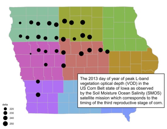
Along with the corn R3 stage there are other agronomic signals contained within Corn Belt VOD, some of which are potentially unique. At present, high-frequency noise in SMOS VOD [10] prevents their identification. Examples of growing-season SMOS VOD in Iowa are shown in Figure 1. Why is SMOS VOD noisy? We have several hypotheses. The retrieval algorithm used by SMOS is a simplification of the actual physics (as it must be to be a useful model) and has been tuned to produce the best soil moisture (and not VOD) retrievals. These soil moisture retrievals have been validated using pixel-scale networks of in situ sensors which make regular measurements of soil moisture over time. No such validation networks of plant water, which could be used to validate VOD, exist. Soil moisture retrievals are also noisy: the soil moisture retrieval uncertainty target for SMOS is $0.04{\mathrm{m}}^3·{\mathrm{m}}^{-3}$ which is significant given the typical range of soil moisture (about $0.45-0.05=0.40{\mathrm{m}}^3·{\mathrm{m}}^{-3}$ [15]). Since SMOS retrieves soil moisture and VOD simultaneously, noise in soil moisture is indicative of noise in VOD because, for a set of observed brightness temperatures, a higher retrieved soil moisture value will correspond to a higher retrieved VOD and a lower retrieved soil moisture value will correspond to a lower retrieved VOD. In addition, satellite pixels at the SMOS spatial scale are heterogeneous with respect to types of land cover and soil type. Parameters used in the soil moisture retrieval algorithm to represent this heterogeneity are uncertain and need further development.

There are also natural factors that may contribute to the noise, such as diurnal variation of plant water. SMOS overpasses occur in the morning and evening. The water potential of plant tissue, and therefore plant water, changes over the course of a day as a result of transpiration, the movement of water from the soil, into plant roots, through a plant’s vascular system, and eventually out of the stomata in its leaves [16]. Hunt et al. [17] observed this diurnal change through the analysis of cellular signals propagating through a field of corn. They found that signal strength was inversely proportional to plant water. A clear diurnal pattern, with plant water being lowest at night and highest in the early afternoon, appeared when the data were detrended to account for the seasonal change. In addition, both dew (often present at 6 am but not 6 pm [18]) and intercepted precipitation contribute to VOD (although Rowlandson et al. [19] could not identify a SMOS dew signal).

Our goal is to model SMOS VOD data in the US Corn Belt to eliminate the noise in the data and reveal new information about crop (and specifically, corn) development. Analyzing SMOS data from 2011 to 2019, we answer three main questions. One, how can we model the seasonal pattern of crop development as measured by SMOS and estimate (and quantify the uncertainty in) key model parameters? Two, how do estimates using SMOS satellite data compare with ground-based USDA NASS estimates of crop development, the only alternative source of information? This is especially important because the USDA stopped reporting the R3 corn stage after the 2013 growing season. Third, what other agronomic information is contained within SMOS VOD?

The remainder of the article is organized as follows. Section 2 details the data used in our investigation, describes our model, and presents a Bayesian approach to estimation. In Section 3, we compare estimated parameters from our model across growing seasons and validate against estimates from USDA survey data. In Section 4, we discuss how our modeling approach could be enhanced, the benefits of our approach, and applications. Finally, in Section 5 we make concluding remarks and present next steps.

2. Data and Methods

The SMOS satellite observes Earth’s brightness temperature via passive microwave (L-band, $f=1.4\mathrm{GHz}$, $\lambda =21\mathrm{cm}$) remote sensing [7]. In the midlatitudes, an individual location is sampled at multiple incidence angles approximately every 12 to 36 hours with overpasses occurring at 6 am and 6 pm local solar time. SMOS VOD, also known as Level 2 τ, is extracted from version 6.5.0 of the SMOS Level 2 Soil Moisture Output User Data Product (MIR_SMUDP2, via https://smos-diss.eo.esa.int/). For a detailed summary of the retrieval algorithm for VOD, see Kerr et al. [8].

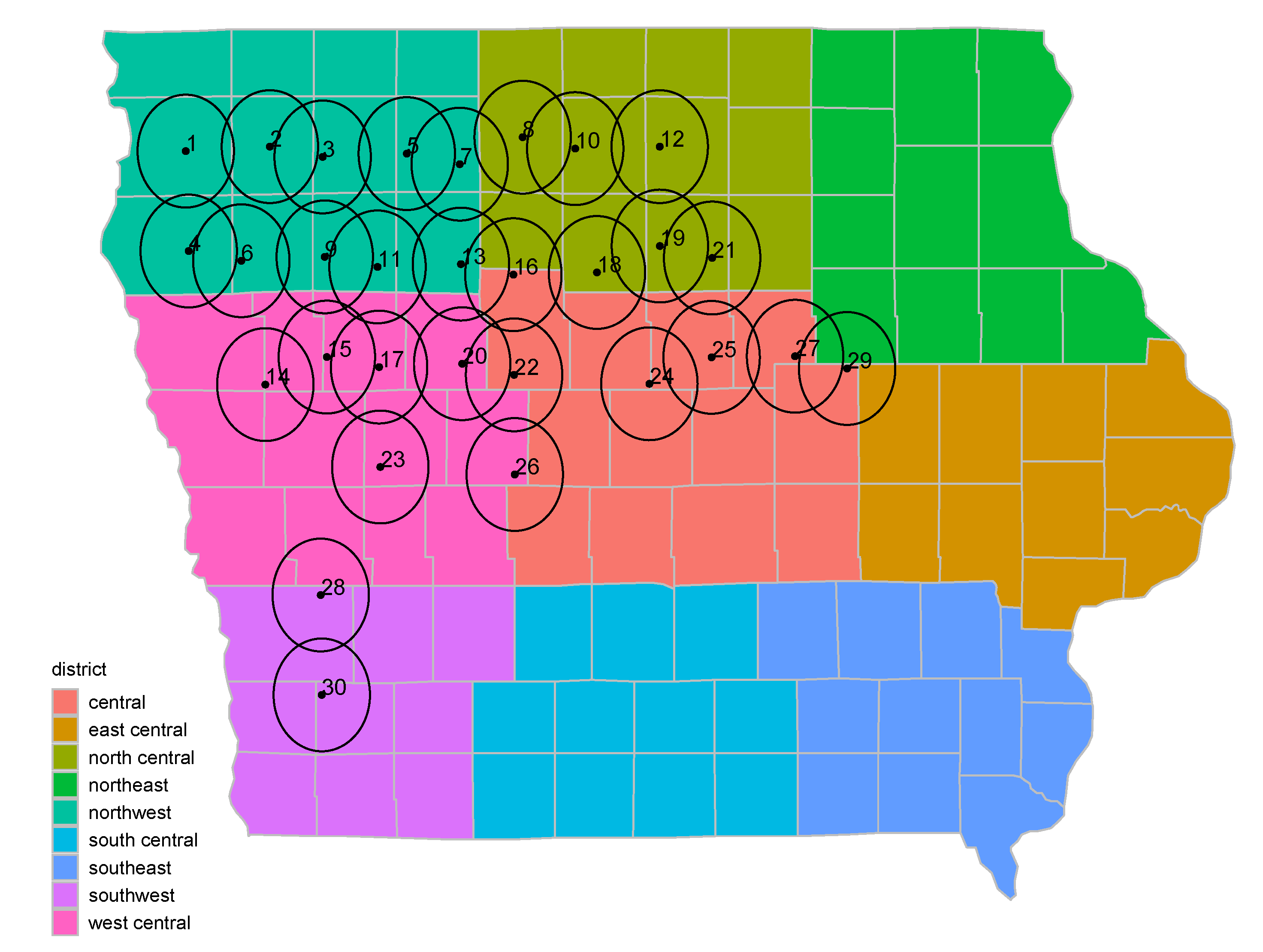
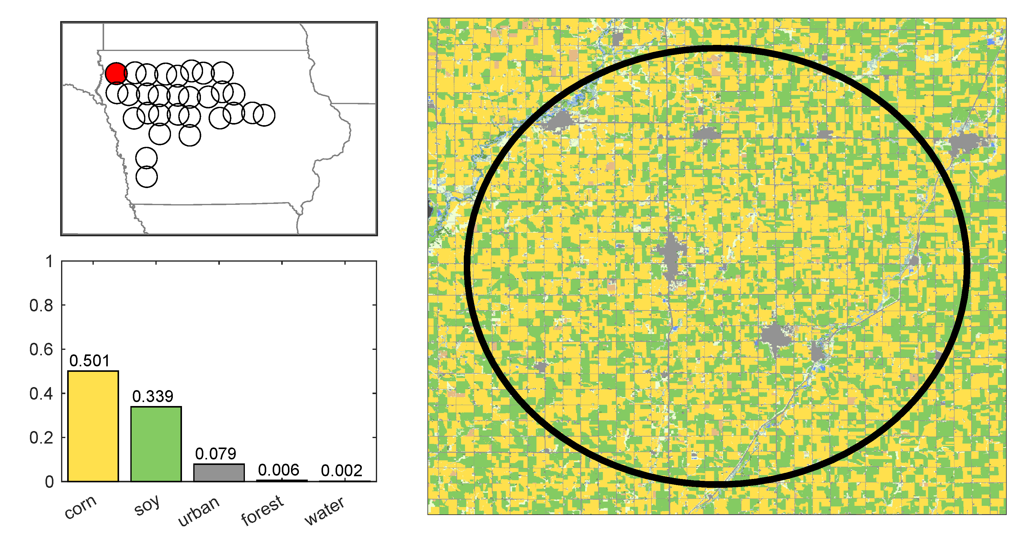
VOD is reported at nadir over a footprint with a consistent centroid but variable diameter, between 40 and 50 km, that is dependent on the location of the footprint within the observation swath. We refer to these footprints as regions and approximate their diameter as 45 km. To minimize the influence of other crops and reduce signal noise from non-agriculture areas, 30 regions were selected in northwest Iowa (Figure 2). Iowa is divided into 99 approximately equal area counties and each region is about the size of a county. All 30 regions have between 75 and 85% of their land area in agricultural row-crops of corn and soybean [20]. Because of the wide spatial resolution of SMOS, individual fields are not identifiable, and many of the regions overlap. However, the overall mixture of crops is consistent across regions and years with approximately 60% of croplands in each region composed of corn and the other 40% soybean [13,21]. Figure 3 presents the USDA NASS 2018 Cropland Data Layer [22] for a region (region 1 in Figure 2) with the average corn and soybean proportion of Hornbuckle et al. [13] (pixel 1 in [13]). Over the years analyzed (2011–2019), based on USDA NASS weekly crop reports (available at https://www.nass.usda.gov/Statistics_by_State/Iowa/Publications/Crop_Progress_&_Condition/index.php), the earliest corn emerged was on the first week in May and by the end of October all corn had reached maturity (R6 growth stage) [23]. We therefore constrain SMOS VOD data in this study from May 1st to October 31st.

Following Walker et al. [24], SMOS retrievals in Iowa have been filtered to remove overpasses where the probability of instantaneous radio frequency interference exceeds 5% (indicating potential anthropogenic contamination) or the ${\chi }^2$ probability is less than 5% (indicating that the retrieval is a poor fit for observed brightness temperatures). Fewer than 3% of VOD retrievals are marked as invalid for each combination of region and season during the study period. VOD is used from both ascending and descending overpasses; in the case of two valid retrievals for a region in a single day the values are averaged to produce a daily measurement.

2.1. Methodology

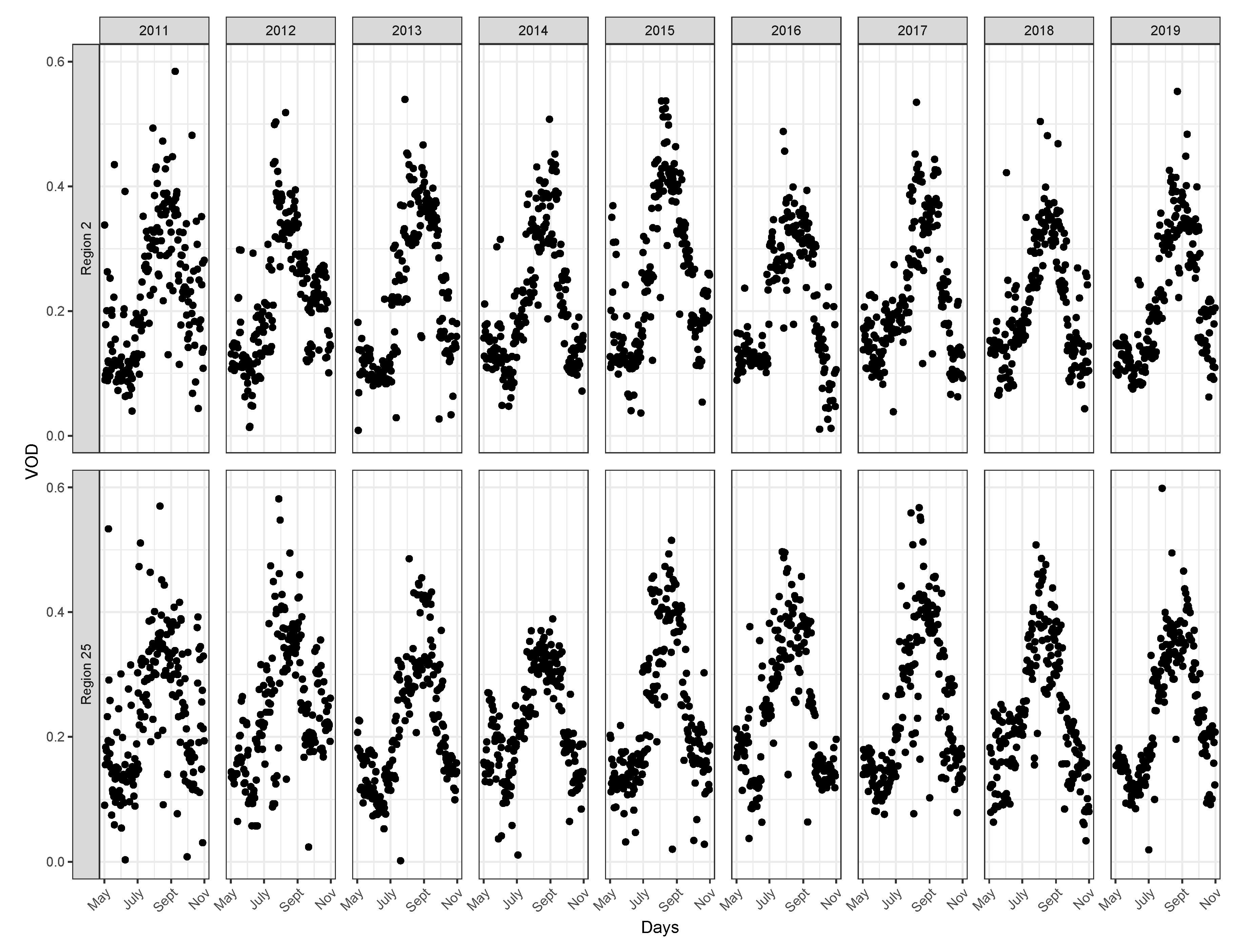
Time series of vegetation indices (e.g., NDVI) that track the growth and senescence of crops exhibit nonlinear behavior: an increase during early to mid-summer as vegetation grows, a peak, and then a gradual decline as crops lose moisture and turn brown. As exemplified in Figure 1, SMOS VOD has a similar asymmetric pattern. Therefore, there is both a theoretical and empirical justification to model VOD using a nonlinear parametric curve.

2.1.1. Data Model for a Single Growing Season

Let $V_{drs}$ be the observed satellite measurement of VOD for region $r=1,\dots ,R=30$ on day $d\in (121,305)$ (May 1 to October 31) of season $s=1,\dots ,S=9$ (corresponding to years 2011 to 2019). We assume $V_{drs}$ is normally distributed with mean $f_{{\theta }_{rs}}\left(d\right)$ and variance ${\nu }_{rs}^2$ as in Equation (1).

$$V_{drs}\stackrel{ind}{\sim }N(f_{{\theta }_{rs}}\left(d\right),{\nu }_{rs}^2)$$

(1)

We define $f_{{\theta }_{rs}}\left(d\right)$ as the value of a parametric function at day d, and ${\theta }_{rs}$ a vector of parameters defining the shape of the curve for region r in season s.

There are multiple nonlinear functions, $f_{{\theta }_{rs}}$, used to model the seasonal signatures of remote sensing vegetation data. We selected the asymmetric Gaussian (AG), also known as the double Gaussian, function. The AG function has been used to describe NDVI data, and often fits better than other curves, such as the double logistic, when compared using empirical data [25,26]. Additional examples using the asymmetric Gaussian function to smooth vegetation data and estimate the dates of key phenological events are found in [27,28].

The full functional form for the AG curve is presented in Equation (2), where the day of the year, d, determines which half of the AG curve is activated. If d is less (greater) than $\delta$ the first (second) Gaussian curve determines the shape of the function on day d [29].

$$f_{\theta }^{AG}\left(d\right)=\left\{\begin{array}{cc}\beta +(\eta -\beta )\exp \left[-\frac{{(d-\delta )}^2}{2{\sigma }_1^2}\right]\hfill & d\le \delta \hfill \\ \beta +(\eta -\beta )\exp \left[-\frac{{(d-\delta )}^2}{2{\sigma }_2^2}\right]\hfill & d>\delta \hfill \end{array}\right.$$

(2)

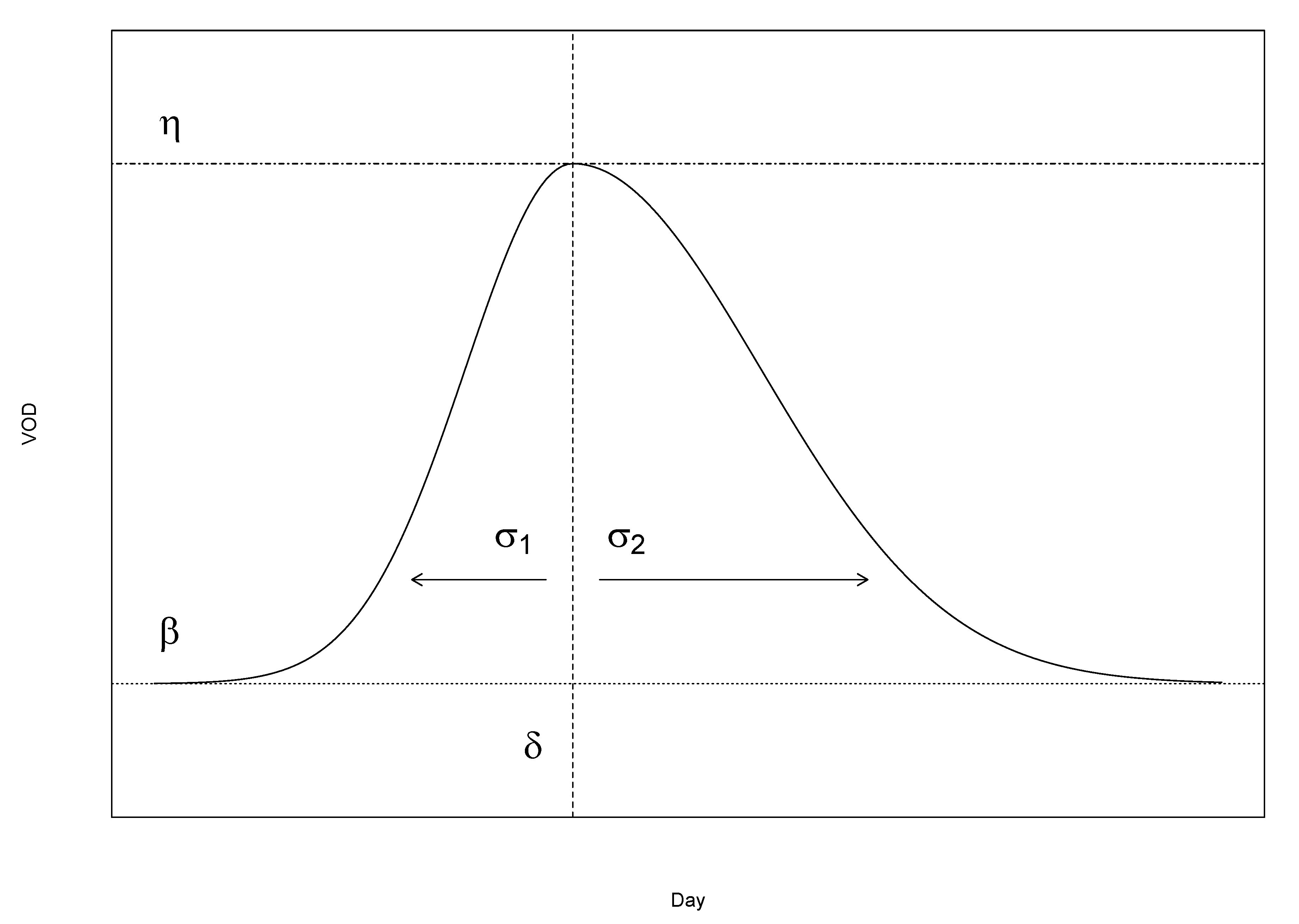
As exemplified in Figure 4, the AG function has the flexibility to capture the nonlinear growth and senescence of crops. Moreover, the parameters of the AG function have meaningful interpretations within the context of the SMOS variable VOD as follows: $\beta$ is the initial steady state or beginning-of-season level of VOD; $\delta$ is the time when the VOD reaches its maximum; $\eta$ is the maximum height of VOD ($\eta >\beta$); ${\sigma }_1$ is the rate at which the crops accumulate tissue water; and ${\sigma }_2$ is the rate at which plant water decreases.

Lastly, a function of the AG parameters that is also of interest to agronomists is the length of the growing season, calculated as $L=({\sigma }_1+{\sigma }_2)\sqrt{2\ln 2}$. In terms of the AG function, this is interpreted as the distance between the left and right inflection points of the AG curve. See [30] for the mathematical derivation.

2.1.2. Borrowing Information across Regions and Seasons

Nonlinear functions are especially sensitive to outliers and noise, a common characteristic of remote sensing data [31]. Therefore, rather than modeling each region individually, we modeled all years and regions jointly within a hierarchical modeling framework. Hierarchical models (also referred to as multilevel models) are useful in applications when the data structure is naturally grouped into multiple nested levels. In the case of the SMOS data, we have a hierarchy with VOD regions nested within growing seasons, and growing seasons nested within the same geographic area. In addition to reflecting the structure of the observations, the hierarchical approach provides a data-based way to borrow information across regions and years to help regularize estimation and produce more stable parameter estimates. For a more detailed summary of hierarchical models, see [32,33].

We further motivate the structure of the hierarchical model as follows. Within a fixed growing season, the parameters defining the nonlinear curve for each region are related due to similar regional weather conditions for that season. Borrowing information across regions provides a more precise estimate of the pattern of crop development within a given growing season. In addition, we can borrow information about the parameters of the curves across growing seasons. Modeling this distribution is important for comparing annual changes in crop development.

Multivariate normal distributions are specified for the season and regional level distributions. We reparameterize the vector of AG parameters in terms of $\theta =(\mathrm{logit}\left(\beta \right),\mathrm{logit}\left(\eta \right),\log \left(\delta \right),\log \left({\sigma }_1\right),\log \left({\sigma }_2\right))$ in order to transform the support of each parameter to the real line. The mean and covariance matrix of the season level distribution is the same for all seasons. For the region level distribution, we allow a separate mean vector for each season but assume a common covariance structure.

We assume the two multivariate normal distributions have different covariance structures to allow for distinct levels of variation in the parameters across, and within, growing seasons. A priori we expect more variation across seasons due to changing environmental conditions. The covariance matrices are modeled in terms of their corresponding standard deviations (${\mathsf{\Lambda }}_{\mu },{\mathsf{\Lambda }}_{\theta }$) and correlation matrices (${\mathsf{\Omega }}_{\mu }$, ${\mathsf{\Omega }}_{\theta }$). This separation approach improves estimation, and provides a more intuitive interpretation of parameter estimates [34]. We define ${\mu }_s=({\mu }_{1s},{\mu }_{2s},{\mu }_{3s},{\mu }_{4s},{\mu }_{5s})$ as the vector of means of the AG parameters for season s, and $\psi =({\psi }_1,{\psi }_2,{\psi }_3,{\psi }_4,{\psi }_5)$ as the overall mean vector for the AG parameters across all growing seasons. Putting the seasonal and region levels together, the full hierarchical model is,

$${\mu }_s\stackrel{ind}{\sim }{N}_5(\psi ,{\mathsf{\Lambda }}_{\mu }{\mathsf{\Omega }}_{\mu }{\mathsf{\Lambda }}_{\mu })\mathrm{and}{\theta }_{rs}\stackrel{ind}{\sim }{N}_5({\mu }_s,{\mathsf{\Lambda }}_{\theta }{\mathsf{\Omega }}_{\theta }{\mathsf{\Lambda }}_{\theta }).$$

(3)

We model the observation errors (${\nu }_s^2$) independently across growing seasons. Within a given season, the satellite noise is roughly the same order of magnitude across regions, so we assume a common seasonal error term.

We now apply this methodology to the SMOS satellite data. To estimate model parameters, we take a Bayesian approach, selecting proper prior distributions to ensure a proper posterior distribution. Because the transformed mean parameters have support over the real line, we use normal prior distributions. Patterns of crop growth are relatively stable, making prior information about the shape of a crop’s growth pattern informative in selecting the location parameters of the prior distributions.

2.2. Prior Distributions

We specify the following prior distributions for the AG model. The intercept (${\psi }_1$) and peak height (${\psi }_2$), receive normal priors $N(-1,1)$ that put 95% of mass between 0.05 and 0.75, which covers reasonable values for the intercept and height of VOD. From historical data we know that corn typically reaches R3 in the middle of August. A normal prior $N(5.5,{\left(0.1\right)}^2)$ for ${\psi }_3$ puts 95% of mass between June 15th and October 15th. This range is approximately plus or minus two months from where we expect the peak to occur so we consider it weakly informative. The two scale parameters (${\psi }_4,{\psi }_5$) receive diffuse normal priors $N(3,1)$. This puts 95% of the mass between 3 and 140, a wide range for the scale parameters given the variable nature of the crop development process which is dependent on weather (and specifically temperature quantified by thermal time e.g., [15]).

For the two correlation matrices, ${\mathsf{\Omega }}_{\mu }$ and ${\mathsf{\Omega }}_{\theta }$, we use the Lewandowski, Kurowicka, and Joe (LKJ) prior with shape parameter 1 which puts a uniform prior over all possible correlation matrices [35]. For the standard deviations of the two covariance matrices (${\mathsf{\Lambda }}_{\mu },{\mathsf{\Lambda }}_{\theta }$), as well as the standard deviations seasonal stochastic error terms (${\nu }_s$), we specify independent half-Cauchy distributions [36,37].

2.3. Model Fitting

Each model was fit using the rstan [38] package in R [39], which implements Hamiltonian Monte Carlo (HMC) [40]. One chain was run for 20,000 iterations with 10,000 used as warmup. The Geweke diagnostic was used to check for adequate mixing [41] using the coda package [42]. There was no evidence of lack of convergence. Traceplots and histograms of the posterior draws were inspected for parameters with the fewest effective samples; these did not suggest features that were inadequately explored. The Supplementary Materials contains histograms of the posterior distributions with priors overlaid on top (Figures S1–S6). For all model parameters, the priors are weakly informative.

3. Results

As detailed in Section 2.1 the parameters of the AG curve have meaningful interpretations in the context of crop development. For the overall seasonal level distribution ($\psi$), the posterior 95% credible intervals (CIs) are presented in

Table 1. 95% CIs for the season level hierarchical parameters ($\psi$).

$\mathit{\beta }$	$\mathit{\eta }$	$\mathit{\delta }$	${\mathit{\sigma }}_1$	${\mathit{\sigma }}_2$
(0.12, 0.14)	(0.34, 0.39)	(217, 237)	(19.40, 33.0)	(21.20, 41.80)

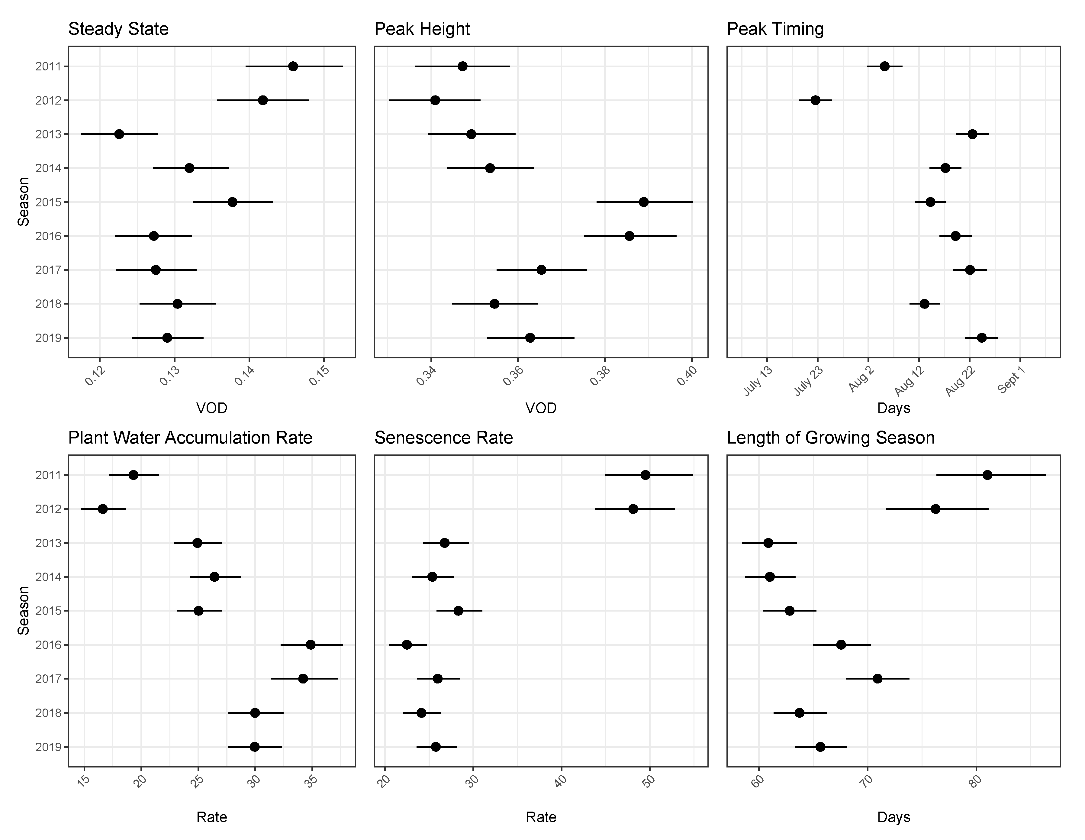
. The intercept ($\beta$) and peak height ($\eta$) have a narrow range suggesting little variation across growing seasons. The timing of the peak has a 95% credible interval covering dates from August 5th to August 24th—a range consistent with USDA historical data for when corn typically reaches R3 [23].

The posterior distribution of the scale parameters is highly correlated with the timing of the peak, and have similar widths of uncertainty. The rate of crop growth (${\sigma }_1$) is slightly smaller than the rate of senescence (${\sigma }_2$). Since smaller values of ${\sigma }_1$ and ${\sigma }_2$ correspond to faster changes, the rates at which plant water accumulates are slightly faster than the rates at which crops dry out.

Looking at the seasonal timing of the peak ($\delta$), we see variation across growing seasons that is supported by other sources of information (Figure 5). For example, 2012 was a notoriously hot summer so corn progressed through its development stages quickly [13]. The 95% CI from our model estimates corn reached its peak growth stage between July 19th to 25th over the 30 regions. In contrast, temperatures cooled in later summer of 2017, resulting in a late harvest [43]. While not statistically significantly different, the median estimate for the peak timing (August 22) in 2017 is later than the previous three years. Iowa’s wettest 12-month period on record (dating back to 1895) occurred from June 2018 until May 2019 [44]. The wet conditions during the spring of 2019 delayed planting and explain why the median value of peak timing in 2019 is later than any other year in the SMOS record.

We can also look at the length of the growing season, L, which measures the length of time for the AG function to reach its peak and return to its initial beginning-of-season steady state value. Using the posterior draws for the shape parameters, this functional is estimable using the relationship described in Section 2.1. Our estimates indicate the 2011 season to have had the longest growth cycle (95% CI: (76, 86)) and 2013 the shortest (95% CI: (58, 63)). Since crops develop according to the accumulation of thermal time (time above a certain base temperature at which no development occurs), weather conditions which vary each year result in different growing season lengths. Our values are consistent with the typical number of calendar days between the early vegetative stages of corn and the late reproductive stages [45].

The two correlation matrices estimate the dependency across the AG parameters. The strongest correlation is between the rate parameters and the timing of the peak height (Figure S5, Supplementary Materials). If crops are developing quickly, they reach R3 faster, and start to dry out earlier as they begin senescence. In addition to improving the precision of model parameters, modeling the correlation structure could be useful for forecasting crop growth mid-season when only partial data are available. Lastly, as expected, the magnitude of the standard deviation parameters of the seasonal level is greater than the standard deviation for the within season distribution, which indicates the crop cycle is more homogeneous between regions within a given year rather than across growing seasons (Figures S3 and S6, Supplementary Materials).

Although we do not know the true timing of maximum VOD, we can compare model estimates to USDA ground-based survey data. The USDA collects data from agronomists and other volunteers (as described in Section 1) and subsets the results into nine reporting districts (Figure 2). Once crops begin to emerge, each week the USDA publishes the percentage of corn (and soybean) at each growth stage by district (

Table 2. Weekly percentage of corn having reached R3 by crop reporting district according to USDA ground-based surveys.

Date	Northwest	North Central	West Central	Central	East Central	Southwest
7/24/11	6	9	7	8	8	7
7/31/11	40	28	33	46	34	34
8/7/11	63	69	70	74	76	64
7/22/12	43	40	33	46	39	26
7/29/12	66	69	69	66	70	75
8/4/13	18	14	18	22	27	25
8/11/13	38	27	55	44	56	49
8/18/13	52	59	71	63	69	73

). Until 2013, the USDA published weekly data on R3, the closest comparable measure to what VOD measures at its peak [13].

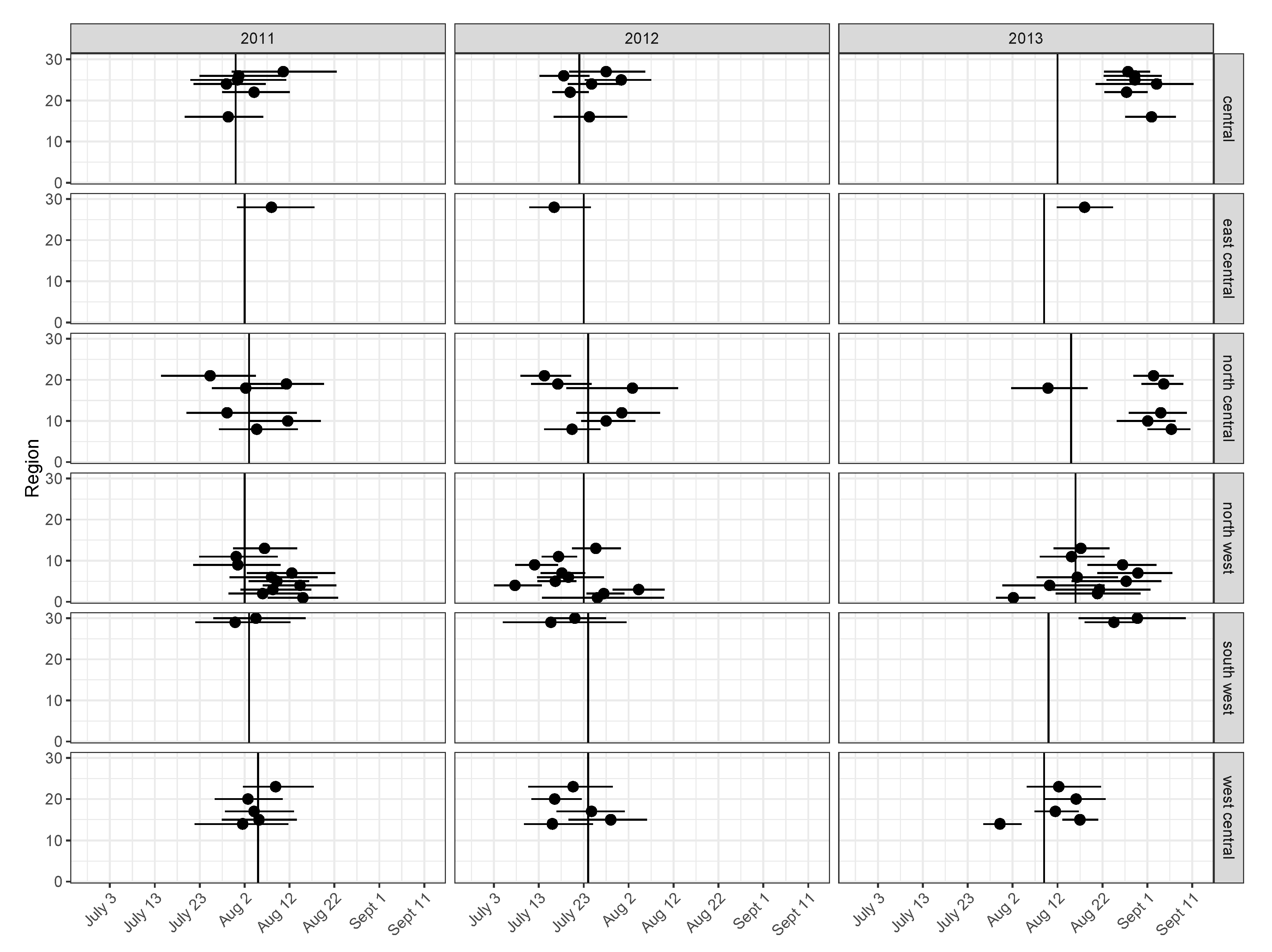
Using linear approximations, we calculated the day of the year when 50% of corn reached R3 for the years 2011 to 2013 (the years R3 estimates and SMOS data overlap) using the data shown in Table 2. We then compared this point estimate to the 95% CIs for peak timing (${\delta }_{rs}$) within the same district. District boundaries are shown in Figure 2. Figure 6 shows the 95% CIs for ${\delta }_{r,2011,2012,2013}$, as well as the USDA 50% R3 estimates, plotted as a vertical line. The bands correspond to the AG model. In 2011 87% (26 of 30 regions) of the AG region CIs overlap with the USDA field data. When we include the 2012 and 2013 seasons, 64% of the CIs for ${\delta }_{r,2011,2012,2013}$ cover the ground-based estimates for our model.

We can also look at the distribution of the timing of peak VOD spatially. Figure 7 plots the median value of the timing of peak VOD for the 2013 growing season. We present the 2013 season as there is more variability in the timing compared to the other seasons shown in Figure 6. There does not appear to be a systematic pattern that can be explained by latitude (e.g., regions further south reaching R3 earlier than regions the northern part of Iowa). However, there is a trend in later dates moving from west-to-east, especially for the northernmost row of estimates. This trend could be caused by progressively later planting dates which in turn could be caused by a precipitation gradient or a gradient in soil temperature during in the spring. There are many other variables that could confound the effect of latitudinal temperature across the state on the timing of peak VOD.

4. Discussion

We first address some important assumptions made in our modeling approach, as well as the use of USDA field survey data as a validation measure. In terms of our parametric model, we assumed the AG function was the correct functional specification for the shape of SMOS VOD curves. We tried two other frequently used nonlinear functions, the double logistic, and Gaussian. The Gaussian was unable to capture the asymmetry of the SMOS data; the double logistic was not significantly better than the AG, and lacks the nice parametric interpretation the AG parameterization offers. Yet, despite trying these two alternatives, there may be other parametric forms outside the remote sensing domain. We also assume exchangeability of regions and growing seasons. Within a fairly small homogeneous region like northwest Iowa this is reasonable. However, it is possible that incorporating the location of the region centroids into a spatial model or adding spatially referenced covariate information (e.g., soil type) could improve parameter estimates. There is additionally an unknown amount of uncertainty in SMOS VOD as the Level 2 retrieval algorithm is a modeled approximation of the land surface with ancillary parameters that are not necessarily representative of the specific region analyzed. To our knowledge, there is not yet published research quantifying the amount of error in VOD using either ground truth validation or simulation-based methods.

The USDA NASS surveys of crop development described in Section 1 are based upon visual observations from roadways, necessitated by the large survey area (e.g., more than 9 million ha of cropland in Iowa alone) and finite number of enumerators. However, the physical characteristics that define all but the first corn reproductive stage can only be determined by directly observing corn ears. The first stage (R1) is “silking” which is when the ear has one or more white string-like silks extending from the top of the corn ear husk. At the second stage (R2) called “blister,” kernels on the ear look like blisters containing a clear fluid. The fluid has a milky appearance at the third stage (R3) or “milk,” and when a corn plant has reached the fourth stage (R4) of “dough” the fluid inside kernels has thickened. As a result, enumerators can only estimate the timing of reproductive stages based upon indirect observable characteristics and their experience. When R3 was reported in Crop Progress and Condition reports the data was described as “in or past milk stage” which reflects its imprecise nature. Therefore, we should only interpret the USDA estimates as an approximation of the true timing of R3.

Our results suggest USDA field-level reporting for estimating when corn reaches R3 could be replaced by the AG model fit to SMOS data, and this estimate would be more accurate than past USDA estimates. We make this claim using inductive reasoning based upon three premises. First, SMOS VOD is directly proportional to plant water in the Corn Belt [14]. Second, corn dominates the total plant water of Corn Belt regions [13]. Third, plant water in corn peaks at the R3 stage [13]. Therefore SMOS VOD should peak at R3. In contrast, USDA estimates are based upon indirect observations. The likely greater accuracy of SMOS VOD is supported by evidence in Figure 6. Note the observations of the timing of peak VOD ($\delta$), and the corresponding USDA estimate of R3, in the central district in 2013. None of the 95% credible intervals of the six values of $\delta$ overlap with the USDA estimate. However, they are consistent with each other. In the north central district in 2013 five of the six regions agree but do not overlap with the USDA estimate. The outlier (region 18 in Figure 2) is still plausible: a significant fraction of this region lies within the central district, and the USDA estimate for the central district is earlier than the north central; $\delta$ for this region is consistent with values in the adjacent northwest district; and since wet soil in the spring delays planting (due to poor trafficability and risk of soil compaction) a region with drier soil conditions would have earlier corn development, and this is certainly possible given the spatial variability of precipitation. The temporal and spatial characteristics of SMOS would result in R3 estimates that could be updated almost daily at a spatial resolution approximately 10 times better than current weekly USDA estimates.

The other parameters estimated by our model are new measures of important agronomic information. The $\beta$ parameter should primarily be a function of soil management. Patton and Hornbuckle [11] determined that pre- and post-season changes in VOD are consistent with changes in soil surface roughness, the mm-scale variations in soil surface height caused by tillage. While tillage increases soil surface roughness, precipitation decreases roughness [46]. Crop residue, the dead plant material that remains on the soil surface after grain is harvested, is also affected by tillage and likely contributes to VOD. In the spring more crop residue is present in reduced tillage cropping systems. Quantifying the amount and spatial variability of residue is of great interest (e.g., [47,48]) because reduced tillage can decrease the transport of soil and chemicals applied as fertilizer out of fields via soil erosion [49]. The VOD should also be sensitive to the presence of cover crops, vegetation planted either after harvest in the fall or before corn and soybean in the spring to reduce soil erosion and immobilize crop nutrients. Reducing the loss of nutrients like nitrogen through increased adoption of reduced tillage and cover crops in the Corn Belt [50] will enhance the water quality of rivers, lakes, and streams and shrink the size of the Dead Zone in the Gulf of Mexico [51]. Changes in the extent and intensity of conservation practices will be reflected in $\beta$. We hypothesize that the difference $\eta -\beta$ is a measure of crop productivity since VOD is a directly proportional to plant water and plant water is related to plant dry matter [14]. The total dry matter accumulation is relevant when crops are grown for biofuel instead of grain. As more energy crops are introduced in the Corn Belt, the VOD might be used to quantify both their in-field economic value and impact on the hydrologic cycle [52]. Data that could be used to validate the $\beta$ and $\eta$ parameters, such as soil surface roughness, the amount of crop residue, and the presence of cover crops, are not routinely collected in the Corn Belt by the USDA or any other state or federal agency at the temporal or spatial scales needed. Instead, future validation work will need to rely on measurements obtained through dedicated field campaigns. Finally, the plant water accumulation rate (${\sigma }_1$) and senescence rate (${\sigma }_2$), and associated growing season length L, are unique to SMOS VOD and need to be explored further.

5. Conclusions

SMOS VOD in the US Corn Belt has potential for monitoring crop growth and development because it is directly proportional to plant water, the mass of water contained within vegetation tissue per ground area. SMOS VOD has several advantages over current visible and near-infrared remote sensing techniques including the fact that clouds are transparent at L-band, peak VOD corresponds directly to a specific crop development stage, signal saturation is not an issue, and near daily measurements are possible. Our goal was to reveal the agronomic information contained within SMOS VOD that is presently hidden by noise. Possible explanations of the noise include a deficient retrieval algorithm and real diurnal changes in plant water.

We found that a nonlinear AG curve was able to describe the seasonal change in VOD. Our approach of modeling curves hierarchically within a season borrows information across satellite measurements taken at different locations; jointly modeling growing seasons borrows data about crop growth patterns across years. This hierarchical structure was critical because fitting stable nonlinear functions to satellite data is problematic due to outliers and noise. Estimation in our model is performed using a Bayesian approach, which provides measures of uncertainty for model parameters with practical importance, such as the timing of the third corn reproductive stage (R3). Although we applied our method to SMOS data, many other vegetation indices exhibit a similar rise and fall over the course of a growing season. Our novel hierarchical approach is generalizable to other remote sensing data.

The parameters of the AG function are new measures of agronomic information. We compared our estimates of the timing of peak VOD, which corresponds to R3, with USDA ground-based survey data and found that in the years 2011, 2012, and 2013, 87%, 70%, and 37% of our estimates coincide, respectively. We postulate that our AG hierarchical model offers a more accurate (as well as less resource-intensive) substitute for this crop stage that was last surveyed by the USDA in 2013 because SMOS VOD corresponds directly to plant water, the mass of water contained within plant tissue per ground area, which corresponds directly to the R3 corn development stage. Moreover, as exemplified in Figure 6 and Figure 7, SMOS VOD captures more local variation in R3 within growing seasons than the USDA provided because the SMOS satellite has a spatial resolution 10 times better than USDA data. Other parameters of the model are functions of soil management and crop productivity and could prove to be useful in assessing the extent of practices that conserve soil and reduce the transport of fertilizer to water bodies, as well as the pre-harvest economic value of biofuels. As SMOS continues to collect data, our model can be used by scientists to better understand how regional climate changes affect agro-ecosystems as well as the adoption rate of new agricultural practices.

There are six main areas of future work. First, our modeling approach could be enhanced by investigating the assumptions discussed in Section 4. Second, our modeling approach should be adapted to also forecast (instead of retro-actively estimate) parameters of the AG function. Third, different corn genotypes (or “hybrids”) are grown throughout the Corn Belt. One way that genotypes vary is in their “maturity rating” or thermal time needed from planting to crop maturity. Since the length of the available growing season (the period between the last and first frost) is primarily a function of latitude, corn with shorter maturity ratings are grown in Minnesota while corn with longer maturity ratings that can take advantage of an extended period of development are grown in Missouri, for example. Although there is no reason to suspect that peak plant water and thus VOD would occur at a different developmental stage in different corn genotypes, this should be verified. Fourth, the relationships between AG parameters $\beta$ and $\eta$ and crop management and productivity need to be established and validated. Fifth, research is needed to interpret maximum and minimum VOD values in other important agricultural regions (as well as other ecosystems) throughout the world. Finally, a better VOD retrieval algorithm could reduce or eliminate noise and make our model obsolete. The current algorithm is based upon the $\tau -\omega$ model which uses two parameters, VOD (also called $\tau$) and the single scattering albedo ($\omega$), to radiometrically characterize a vegetation canopy (e.g., [53]). The $\tau -\omega$ model is a zero-order solution of the radiative transfer equation only appropriate for limited canopy volume scattering. A new VOD retrieval algorithm may need to consider multiple scattering induced by crop components (such as stems) that are of significant electrical size at L-band. It is also possible that diurnal changes impacting VOD (e.g., plant water hydraulics, dew) could be important. The development of a such an algorithm that is still useful at the satellite scale will be difficult but could provide a wealth of new agronomic information across the Corn Belt and other agricultural regions.