Moreau-Enhanced Total Variation and Subspace Factorization for Hyperspectral Denoising

Abstract

Hyperspectral images (HSIs) denoising aims at recovering noise-free images from noisy counterparts to improve image visualization. Recently, various prior knowledge has attracted much attention in HSI denoising, e.g., total variation (TV), low-rank, sparse representation, and so on. However, the computational cost of most existing algorithms increases exponentially with increasing spectral bands. In this paper, we fully take advantage of the global spectral correlation of HSI and design a unified framework named subspace-based Moreau-enhanced total variation and sparse factorization (SMTVSF) for multispectral image denoising. Specifically, SMTVSF decomposes an HSI image into the product of a projection matrix and abundance maps, followed by a ‘Moreau-enhanced’ TV (MTV) denoising step, i.e., a nonconvex regularizer involving the Moreau envelope mechnisam, to reconstruct all the abundance maps. Furthermore, the schemes of subspace representation penalizing the low-rank characteristic and ${\ell }_{2,1}$-norm modelling the structured sparse noise are embedded into our denoising framework to refine the abundance maps and projection matrix. We use the augmented Lagrange multiplier (ALM) algorithm to solve the resulting optimization problem. Extensive results under various noise levels of simulated and real hypspectral images demonstrate our superiority against other competing HSI recovery approaches in terms of quality metrics and visual effects. In addition, our method has a huge advantage in computational efficiency over many competitors, benefiting from its removal of most spectral dimensions during iterations.

1. Introduction

With the wealth of spatial and spectral information, hyperspectral image (HSI) delivers a more accurate description ability of real scenes to distinguish precise details than color images and provides potential advantages of application in vegetation monitoring, medical diagnosis, mineral exploration, among numerous others [1,2]. However, due to the instrument restrictions and various weather conditions, HSIs are unavoidably corrupted by complicated forms of noise during the acquisition procedure [3], which significantly plagues the subsequent applications, such as classification [4], spectral unmixing [5,6], and anomaly detection [7,8]. As a result, denoising the HSIs become an essential preprocessing step to support the subsequent HSI-related applications and analysis.

There is ever-growing attention in HSI denoising and numerous approaches have been developed in recent decade. A straightforward approach is to use a classical gray-level image restoration method for HSI in a bandwise manner. See, e.g., [9,10,11]. However, this strategy always leads to unsatisfactory results as the correlations among adjacent bands or pixels have been ignored. Aiming at improving the recovery quality, scholars turn to simultaneously encode the spatial and spectral correlation knowledge for a natural HSI. For example, a spatial-spectral adaptive total variation model is proposed in [12]; a cubic TV (CTV) model is designed in [13]; a nonlocal sparse representation framework is developed in [14]. In addition, as a data cube, the tensor filtering technique is exploited for HSI denoising, such as multidimensional Wiener filtering (MWF) [15] and Block-Matching 4D filtering (BM4D) [16]. However, due to the lack of the consideration of deeper prior knowledge, these methods often result in suboptimal performance in eliminating mixed noise.

Inspired by the redundancy of the HSI spectral bands, low-rank technology has been widely accepted and applied to HSI processing. Assuming HSIs underlie a low-dimensional spectral subspace with certain predefined low-rank constraint, the matrix approximation/factorization method becomes representative work of restoring the pure HSI image from its degraded observation. Based on the robust PCA (RPCA) framework [17], Zhang et al. [18] employ a low-rank matrix recovery (LRMR) model for HSI denoising. He et al. [19] improve the patch-wise LRMR with a noise-adjusted iterative low-rank matrix approximation strategy, in which the different noise variance crosses the spectral bands are taken into account. To further enhance the restoration quality, many nonconvex low-rank regularizers, such as weighted Schatten p-norm (WSN) [20], $\gamma$-norm [21], are introduced into the matrix approximation framework instead of the original nuclear norm minimization. By projecting the original image into a spectral difference space, Sun et al. [22] put forward another type of low-rank approximation method for noise reduction, which gets out of the trouble of treating sparse noise as a low-rank feature. Song et al. [23] introduce adaptive dictionary learning into the sparse representation to solve the denoising problem. In addition, other low-rank-based methods, including superpixel segmentation [24], and spectral nonlocal property [25], also have superior performance to this end. However, the drawback of all the aforementioned methods is that, after vectorizing the HSI bands, the following steps would be sensitive to outliers and fail to completely get rid of the structured stripes and deadlines. On the other hand, low-rank tensor-based approaches have also been proposed for HSI denoising, for maintaining the global spatial-spectral structure. See, e.g., [26,27,28,29,30] among others. However, as presented in [31], most existing tensor-based HSI denoising methods still lead to noisy recovery results, especially under heavy mixed-noise scenarios.

To improve the spatial resolution, many conventional spatial regularizers, such as total-variation [32] and nonlocal similarity [3,14], are integrated into the low-rank based method for separating the noise component from the image component and promoting smoothness. Total variation (TV) regularization shows remarkable performance for image reconstruction and is one of the most representatives sparsity promotion techniques. Therefore, various types of TV regularization have been adopted to denoise the HSIs. The work [31] combines band manner TV into the low rank model to induce sparsity more effectively, thereby enhancing the denoising performance. Wu et al. [33] incorporate TV regularization in the weighted nuclear norm minimization (WNMM) [34] framework to explore the spatial prior of HSI. However, bandwise TV neglects the intrinsic characteristics of the spectral piecewise smoothness within the HSI. To remedy this problem, by expanding the traditional TV model, three-dimensional TV (3DTV) [35] and spatio-spectral TV (SSTV) [36,37] have been widely adopted to better maintain the spatial and spectral smoothness. Li et al. [38] present an HSI destriping method by combining adaptive moment matching with multi-level unidirectional total variational. In addition, in [28], the structure tensor TV proposed by Lefkimmiatis et al. [39] is further introduced into the WNNM model, and achieves superior recovery performance compared to their previous work [33].

One notable fact is that most of the published LR-based hyperspectral denoising algorithms explore the low-rank approximation in the large size spectral dimension at the expense of computational efficiency. Fortunately, subspace-based HSI denoising methods provide a new perspective to cope with this problem. Much information in HSI data can be obtained by linearly combining some endmembers with a set of sparse coefficients. For this reason, global spectral low-rank priors can be enforced by using subspace representation. The projection-based method is first presented by Zhuang and Bioucas-Dias [40] for Gaussian and Poissonian noise removal. In [41], low-rank tensor factorization is further introduced into the subspace representation framework for HSI self-similar property enhancement. He et al. [42] transfer the non-local denoising to the projected HSI instead of the original spectral dimension to reduce processing cost. However, the methods mentioned above cannot handle structural sparse noise. Therefore, the denoising performance based on subspace representation still has room for improvement.

Motivated by such studies, a non-separable non-convex TV denoising penalty combined with the subspace representation framework is proposed to recover HSI from mixed noise. We first decompose the original HSI as a subspace matrix multiplied by coefficients matrix and subsequently explore the spatial piecewise smoothness effectively in the projected space. Specifically, the non-separable non-convex TV penalty is generated based on the Moreau envelope, which follows a similar idea proposed in our previous paper [43]. Our main contributions are as follows:

• The low-rank structure of HSI data are explored via subspace representation, which is realized by decomposing the HSI into the product of projection matrix and abundance maps. To separate the noise out, the projection matrix is required to be orthogonal.
• The Moreau-enhanced TV as a non-convex regularizer is applied to each abundance map, which is expected to enhance the spatial information and thus achieve more performance boost. Furthermore, subspace representation and ${\ell }_{2,1}$-norm are incorporated into our denoising framework.
• A variational augmented Lagrangian method (ALM) algorithm is designed to minimize the proposed model. Extensive experiments confirm that our method can offer an excellent recovery performance compared with many popular HSI denoising methods. More importantly, the proposed algorithm requires less computational cost than most others.

This paper is organized as follows. Section 2 reviews the HSI degradation model and some related works. Section 3 presents the proposed Moreau-enhanced total variation and subspace factorization model, followed by its optimization solution. Various experimental results including comparisons with other competing methods are reported in Section 4. The final section gives our conclusions.

2. Background Formulation

2.1. Problem Formulation

Let $\mathcal{Y}\in {\mathbb{R}}^{p\times h\times w}$ represent an observed HSI data with p spectral bands of spatial size $h\times w$. In this study, the 3D HSI image is rearranged as a 2D matrix $\mathbf{Y}\in {\mathbb{R}}^{p\times l}(l=h\times w)$ for the purpose of easier analysis, where each row contains a vectorized spectral channel band. Following the studies of [31,37], HSIs are assumed to be contaminated by mixed noise, and its noisy observation can be described in a matrix form as

$$\begin{array}{c}\hfill \begin{array}{c}\hfill \mathbf{Y}=\mathbf{X}+\mathbf{S}+\mathbf{N},\end{array}\end{array}$$

(1)

where X represents the clean HSI; S denotes sparse error term, representing a mixture of impulse noise and outliers; and N is the Gaussian noise. The images X, S, and N are modeled the same way as Y. The goal of HSI denoising is to separate the noise from observed image with proper constraints.

Under the assumption of image degradation model (1), the generalization model for estimating the clean image X is designed as

$$\begin{array}{c}\hfill \begin{array}{c}\hfill \left\{\widehat{\mathbf{X}},\widehat{\mathbf{S}}\right\}=\underset{\mathbf{X},\mathbf{S}}{argmin}\frac{1}{2}\parallel \mathbf{Y}-\mathbf{X}-\mathbf{S}{\parallel }_{\mathit{F}}^2+{\lambda }_{\mathit{1}}{\mathit{J}}_1\left(\mathbf{X}\right)+{\lambda }_{\mathit{2}}{\mathit{J}}_2\left(\mathbf{S}\right),\end{array}\end{array}$$

(2)

where the first term is the data-fidelity term, which represents the similarity between the restored image and degraded image, and ${\parallel ·\parallel }_{\mathit{F}}$ denotes the Frobenius norm. ${\mathit{J}}_1\left(\mathbf{X}\right)$ is a regularization term describing the intrinsic structure of the image component, e.g., non-local similarity [44], global low-rank property [45]. ${\mathit{J}}_2\left(\mathbf{S}\right)$ is the sparse regularization characterizing the prior knowledge of the sparse corruptions. ${\lambda }_1$ and ${\lambda }_2$ are two predefined scalar parameters used to balance the contribution of each relevant term. Therefore, the core of image denoising is how to exactly exploit the prior information for both X and S to effectively separate the noise components.

2.2. Global Low-Rank Matrix Factorization

HSIs are well-known for holding strong spectral low-rank characteristic. This suggests that each spectral signature (columns of X) lies in a common k-dimensional subspace ${\mathcal{S}}_k$. As stated in [46,47], the value of k is far less than the spectral dimension, i.e., p≫k. Therefore, the target image X can be presented as $\mathbf{X}=\mathbf{AM}$, where $\mathbf{A}\in {\mathbb{R}}^{p\times k}$ represents the basis of the subspace ${\mathcal{S}}_k$, hereafter termed projection matrix, and $\mathbf{M}\in {\mathbb{R}}^{k\times l}$ is regarded as the coefficient matrix. In many real situations, both A and M have evident physical meanings. Specifically, the columns of A are the spectral signatures (endmembers), and M is the abundance fraction vector. According to the idea presented in [40], the projection matrix A is required to be orthogonal, i.e., $\mathbf{A}{}^{\mathit{T}}\mathbf{A}=\mathbf{I}$, and it can be obtained by singular value decomposition (SVD) or other signal subspace identification approaches [48] of hyperspectral imagery.

As a consequence, the HSI data can be modeled as

$$\begin{array}{c}\hfill \begin{array}{c}\hfill \mathbf{Y}=\mathbf{AM}+\mathbf{S}+\mathbf{N}.\end{array}\end{array}$$

(3)

Following [42], the orthogonal constraint $\mathbf{A}{}^{\mathit{T}}\mathbf{A}=\mathbf{I}$ can keep noise out of A and help to further refine the abundance map iteratively. By incorporating the orthogonal constraint into the model (2), the corresponding HSI restoration model is denoted as

$$\begin{array}{c}\hfill \begin{array}{cc}\hfill \left\{\widehat{\mathbf{A}},\widehat{\mathbf{M}},\widehat{\mathbf{S}}\right\}=& \underset{\mathbf{A},\mathbf{M},\mathbf{S}}{argmin}\frac{1}{2}\parallel \mathbf{Y}-\mathbf{AM}-\mathbf{S}{\parallel }_{\mathit{F}}^2+{\lambda }_{\mathit{1}}{\mathit{J}}_1\left(\mathbf{M}\right)+{\lambda }_{\mathit{2}}\parallel \mathbf{S}\parallel {}_{2,1}\mathrm{s}.\mathrm{t}.{\mathbf{A}}^{\mathit{T}}\mathbf{A}=\mathbf{I},\hfill \end{array}\end{array}$$

(4)

where ${\mathit{J}}_1\left(\mathbf{M}\right)$ describes the prior information of the abundance map and $\parallel ·\parallel {}_{2,1}$ refers to the ${\ell }_{2,1}$-norm, which is associated with the sparse noise of the spatial difference images. It should be also pointed out that model (4) includes capturing the global correlation along spectrum as well as reducing the computational burden.

3. Proposed Method

3.1. Moreau-Enhanced TV Restoration Model

TV-based regularization is well known to enforce piecewise smoothness and has been successfully used in HSI processing [31,37]. Denoting the image domain as $\mathbf{y}\in {\mathbb{R}}^{\mathit{h}\times \mathit{w}}$, the general image restoration model of linear total variation function is formulated as

$$\begin{array}{ll}\hfill \mathrm{tvd}(\mathbf{y};\eta )& =\underset{\mathbf{x}}{argmin}\left\{\frac{1}{2}\parallel \mathbf{y}-\mathbf{x}{\parallel }_F^2+\eta {\parallel \mathbf{x}\parallel }_{\mathrm{TV}}\right\},\eta >0\\ & ={\mathbf{prox}}_{\eta {\parallel ·\parallel }_{\mathrm{TV}}}\left(\mathbf{y}\right),\end{array}$$

(5)

which claims that TV restoration model can be regarded as the proximity operator of x $\mapsto \parallel \mathbf{x}{\parallel }_{\mathrm{TV}}$. $\eta$ is a regularization parameter that maintains the trade-off between the Frobenius norm and the TV norm. To precisely preserve the local piecewise continuity and induce sparsity more efficiently than the TV norm, we define a non-differentiable non-convex penalty suitable for TV denoising model, i.e.,

$$\begin{array}{c}\hfill \begin{array}{c}\hfill {\Psi }_{\alpha }\left(\mathbf{x}\right)={\parallel \mathbf{x}\parallel }_{\mathrm{TV}}-{\mathit{S}}_{\alpha }\left(\mathbf{x}\right),\end{array}\end{array}$$

(6)

where ${\mathit{S}}_{\alpha }\left(\mathbf{x}\right)$ indicates the Moreau envelop of ${\parallel ·\parallel }_{\mathrm{TV}}$ with index 1/$\alpha$ as the threshold ($\alpha >0$), and is defined as

$$\begin{array}{c}\hfill \begin{array}{c}\hfill {\mathit{S}}_{\alpha }\left(\mathbf{x}\right)=\underset{\mathbf{u}}{argmin}\left\{{\parallel \mathbf{u}\parallel }_{\mathrm{TV}}+\frac{\alpha }{2}{\parallel \mathbf{x}-\mathbf{u}\parallel }_2^2\right\}.\end{array}\end{array}$$

(7)

Proposition 1.

Let$\alpha \ge$0, the function${\mathit{S}}_{\alpha }\left(\mathbf{x}\right)$is convex and differentiable. Its gradient$\nabla {\mathit{S}}_{\alpha }\left(\mathbf{x}\right)$can be expressed as

$$\begin{array}{c}\hfill \begin{array}{c}\hfill \nabla {\mathit{S}}_{\alpha }\left(\mathbf{x}\right):=\left\{\begin{array}{cc}0,\hfill & \alpha =0,\hfill \\ \alpha \left(\mathbf{x}-{\mathbf{prox}}_{\frac{1}{\alpha }{\parallel ·\parallel }_{\mathrm{TV}}}\left(\mathbf{x}\right)\right),\hfill & \alpha >0.\hfill \end{array}\right.\end{array}\end{array}$$

(8)

Proof. 

From the Proposition 12.15 of [49], ${\mathit{S}}_{\alpha }\left(\mathbf{x}\right)$ is convex, real-valued, continuous, and exact since ${\mathit{S}}_{\alpha }\left(\mathbf{x}\right)$ is the Moreau envelop of ${\parallel ·\parallel }_{\mathrm{TV}}$ with index 1/$\alpha$. Similarly, from the Proposition 12.29 of [49], ${\mathit{S}}_{\alpha }\left(\mathbf{x}\right)$ is differentiable. When $\alpha >0$, we get

$$\begin{array}{c}\hfill \begin{array}{c}\hfill \nabla {\mathit{S}}_{\alpha }\left(\mathbf{x}\right)=\alpha \left(\mathbf{x}-{\mathbf{prox}}_{\frac{1}{\alpha }{\parallel ·\parallel }_{\mathrm{TV}}}\left(\mathbf{x}\right)\right).\end{array}\end{array}$$

(9)

For $\alpha =0$, ${\mathit{S}}_0\left(\mathbf{x}\right)=0$. Following with the definition of gradient, we have $\nabla {\mathit{S}}_0\left(\mathbf{x}\right)=0$. Thus, we obtain the proposition.

Simultaneously, if $\alpha >0$, ${\Psi }_{\alpha }\left(\mathbf{x}\right)$ is non-convex, and the ‘degree of concavity’ of the functional ${\Psi }_{\alpha }\left(\mathbf{x}\right)$ is controlled by the value of scalar coefficient $\alpha$. When $\alpha =0$, model (6) reverts to the classical TV penalty. Compared with TV norm, if $\alpha >0$, the new penalty can more accurately determine the jumps of the piecewise constant image.

To strongly induce sparsity, we introduce the new penalty function ${\Psi }_{\alpha }\left(\mathbf{x}\right)$ as the piecewise smoothness surrogate to substitute the TV norm in (5). Consequently, the Moreau-enhanced TV denoising model is formulated as

$$\begin{array}{c}\hfill \begin{array}{c}\hfill \mathrm{mtvd}(\mathbf{y};\eta ,\alpha )=\underset{\mathbf{x}\in {\mathbb{R}}^{\mathit{m}\times \mathit{n}}}{argmin}\left\{\frac{1}{2}\parallel \mathbf{y}-\mathbf{x}{\parallel }_{\mathrm{F}}^2+\eta {\Psi }_{\alpha }\left(\mathbf{x}\right)\right\},\eta >0,\end{array}\end{array}$$

(10)

where the parameter $0\le$$\alpha$$\le 1/\eta$ is such that the model (10) is convex; $0\le \alpha <1/\eta$ is such that the model (10) is strictly convex. For the non-convex analysis of model (10), we refer the readers to [50] and the references therein. When model (10) is strongly convex, the minimizer problem can be efficiently solved by the forward-backward splitting (FBS) algorithm [49]. Its solution is given in Appendix A.

3.2. Subspace-Based Moreau-Enhanced TV Restoration Model

According to the description of Section 2.2, matrix $\mathbf{M}\in {\mathbb{R}}^{k\times l}$ can be inferred from the projection of the observed HSI Y onto subspace A, i.e., $\mathbf{M}=\mathbf{A}{}^{\mathit{T}}\mathbf{Y}$. In addition, the dimension k of subspace A can be estimated by HySime [48] (We give the reference of the HySime algorithm). The details can be found in Appendix B. According to [51], the abundance map inherits two important properties of the original image, namely sparsity and piecewise smooth structure. To guarantee lower complexity and better performance, in this paper, ‘Moreau-enhanced’ TV denoising technique is applied on matrix $\mathbf{M}$ to preserve the above-mentioned two characteristics concurrently.

After defining the ‘Moreau-enhanced’ TV denoising model in Section 3.1, we treat it as a prior and process abundance maps in a band-wise manner. Mathematically, abundance maps denoising can be reformed as

$$\begin{array}{c}\hfill \begin{array}{c}\hfill \widehat{\mathbf{L}}=\underset{\mathbf{L}}{argmin}\sum _{i=1}^{\mathit{k}}\left\{\frac{1}{2}\parallel \mathcal{F}{\mathbf{M}}^i-\mathcal{F}{\mathbf{L}}^i{\parallel }_F^2+\eta {\Psi }_{\alpha }\left(\mathcal{F}{\mathbf{L}}^i\right)\right\},\eta >0,\end{array}\end{array}$$

(11)

in which ${\mathbf{M}}^i$ represents the row vector of the abundance matrix, $\mathcal{F}$: ${\mathbb{R}}^l\to {\mathbb{R}}^{h\times w}$ denotes the operation reshaping a vector to a 2D matrix with a size of $h\times w$, and L represents the denoised result. To verify the superiority of ‘Moreau-enhanced’ TV denoising model (Equation (10)) over TV denoising model (Equation (5)), we utilize the two models to restore the abundance matrix M and projection A (shown in Figure 1), which are derived from the corrupted Washington DC Mall image (WDC) with noise variance 0.2. Reference M(:, 4) and A(:, 4) are estimated from the clean image. Here, A(:, i) is the i-th characteristic of HSI and the corresponding coefficient matrix M(:, i) is the abundance map. By comparing the original noiseless image, we can see that the denoised results of the TV denoising model are still suffering from the noise.

Simplifying model (11) yields the following representation:

$$\begin{array}{c}\hfill \begin{array}{c}\hfill \widehat{\mathbf{L}}=\sum _{i=1}^{\mathit{k}}\mathrm{mtvd}(\mathcal{F}{\mathbf{M}}^{\mathrm{i}};\eta ,\alpha ),\eta >0.\end{array}\end{array}$$

(12)

With all these, the proposed SMTVSF HSI denoising model can be written as follows:

$$\begin{array}{c}\hfill \begin{array}{ccc}\hfill \left\{\widehat{\mathbf{A}},\widehat{\mathbf{M}},\widehat{\mathbf{S}}\right\}=\underset{\mathbf{A},\mathbf{M},\mathbf{S}}{argmin}\frac{1}{2}\parallel \mathbf{Y}& -\mathbf{AM}-\mathbf{S}{\parallel }_{\mathit{F}}^2+{\lambda }_{\mathit{1}}\sum _{\mathrm{i}=1}^{\mathit{k}}\mathrm{mtvd}(\mathcal{F}{\mathbf{M}}^{\mathrm{i}};\eta ,\alpha )+{\lambda }_{\mathit{2}}\parallel \mathbf{S}\parallel {}_{2,1}\hfill & \mathrm{s}.\mathrm{t}.{\mathbf{A}}^{\mathit{T}}\mathbf{A}=\mathbf{I},\eta >0,\end{array}\end{array}$$

(13)

where ${\lambda }_1$ controls the contribution of ‘Moreau-enhanced’ TV denoising model, and ${\lambda }_2$ controls the weight of the sparsity term. Theoretically, the second term of model (13) will degenerate into the band-by-band TV denoising model when $\alpha$ is set to 0.

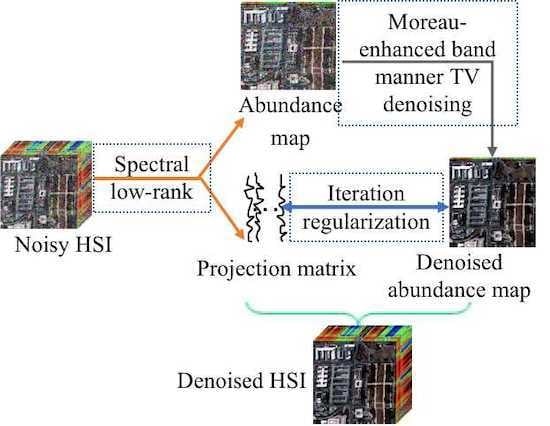
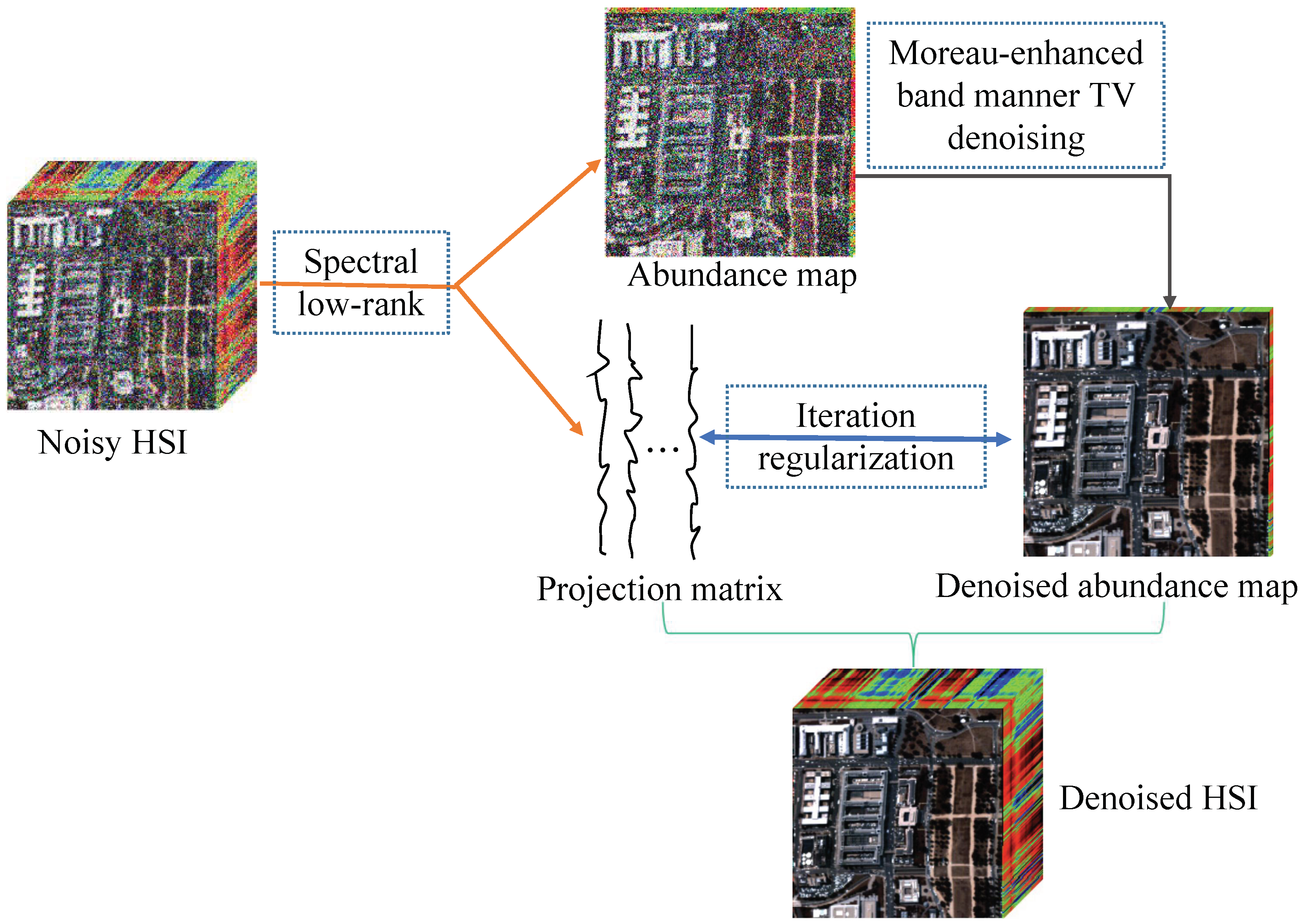
Our final model unifies matrix factorization, Gaussian noise removal, and sparse noise elimination in a framework; thus, it is expected to have a strong ability to separate mixed noise from the degraded image. The basic idea of the model is to first transform the observed HSI into certain low-dimensional space, and subsequently recover the spatial detail information of the projected HSI. To enhance the performance, we refine the abundance maps and projection space during the iteration. Then, the restored HSI is obtained via inverse transformation. Figure 2 illustrates the overview of the proposed method.

3.3. Optimization Procedure

The proposed method is mainly composed of three components: spectral low-rank projection; spatial domain denoising; and sparsity constraint of the sparsity noise. The details of the first step can be found in Section 2.2. The solution of the other two steps is presented in the following.

(1) Spatial denoising via abundance maps: In this stage, the ‘Moreau-enhanced’ TV regularized method is applied to the abundance map instead of the whole spectral image to reduce the calculation cost. The objective in this stage is

$$\begin{array}{c}\hfill \begin{array}{c}\hfill \widehat{\mathbf{L}}=\underset{\mathbf{L}}{argmin}\sum _{i=1}^{\mathit{k}}\left\{\frac{1}{2}\parallel \mathcal{F}{\mathbf{M}}^i-\mathcal{F}{\mathbf{L}}^i{\parallel }_F^2+\eta {\Psi }_{\alpha }\left(\mathcal{F}{\mathbf{L}}^i\right)\right\},\eta >0.\end{array}\end{array}$$

(14)

The parameter $\alpha$ affects the denoising performance and we analyze the influence of parameter $\alpha$ in Section 4.3. It should be noted that ${\Psi }_{\alpha }\left(\mathbf{x}\right)$ degrades into the standard TV penalty when $\alpha$ is set to 0. Then, the above model (14) can be converted into k standard 2D TV denoising problems:

$$\begin{array}{c}\hfill \begin{array}{c}\hfill \widehat{\mathbf{L}}=\underset{\mathbf{L}}{argmin}\sum _{i=1}^{\mathit{k}}\left\{\frac{1}{2}\parallel \mathcal{F}{\mathbf{M}}^i-\mathcal{F}{\mathbf{L}}^i{\parallel }_F^2+\eta \parallel \mathcal{F}{\mathbf{L}}^i{\parallel }_{\mathrm{TV}}\right\},\eta >0.\end{array}\end{array}$$

(15)

(2) Iterative refinement: After obtaining the coarse denoised projected HSI $\mathbf{L}$, the restoration model in this stage becomes

$$\begin{array}{c}\hfill \begin{array}{cc}\hfill \left\{\widehat{\mathbf{A}},\widehat{\mathbf{M}},\widehat{\mathbf{S}}\right\}& =\underset{\mathbf{A},\mathbf{M},\mathbf{S}}{argmin}\frac{1}{2}\parallel \mathbf{Y}-\mathbf{AM}-\mathbf{S}{\parallel }_{\mathit{F}}^2+{\lambda }_{\mathit{1}}\sum _{\mathrm{i}=1}^{\mathit{k}}\frac{1}{2}\parallel \mathcal{F}{\mathbf{M}}^{\mathit{i}}-\mathcal{F}{\mathbf{L}}^{\mathit{i}}{\parallel }_{\mathrm{F}}^2+{\lambda }_{\mathit{2}}\parallel \mathbf{S}\parallel {}_{2,1}\mathrm{s}.\mathrm{t}.{\mathbf{A}}^{\mathit{T}}\mathbf{A}=\mathbf{I}.\hfill \end{array}\end{array}$$

(16)

For solving model (16), we introduce the ALM methodology [52] to minimize the following model:

$$\begin{array}{c}\hfill \begin{array}{c}\hfill \left\{\widehat{\mathbf{A}},\widehat{\mathbf{M}},\widehat{\mathbf{S}}\right\}=\underset{\mathbf{A},\mathbf{M},\mathbf{S}}{argmin}\frac{1}{2}\parallel \mathbf{Y}-\mathbf{AM}-\mathbf{S}{\parallel }_{\mathit{F}}^2+{\lambda }_{\mathit{1}}\sum _{\mathrm{i}=1}^{\mathit{k}}\frac{1}{2}\parallel \mathcal{F}{\mathbf{M}}^{\mathit{i}}-\mathcal{F}{\mathbf{L}}^{\mathit{i}}{\parallel }_{\mathrm{F}}^2+{\lambda }_{\mathit{2}}\parallel \mathbf{S}\parallel {}_{2,1}+{\zeta }_{{\mathbf{I}}_{\mathit{k}}}\left(\mathbf{A}{}^{\mathit{T}}\mathbf{A}\right).\end{array}\end{array}$$

(17)

Subsequently, we split the multivariable optimization problem (17) into several manageable subproblems and the solution of the corresponding subfunctions can be established in an alternating minimization manner.

(1) The update of S is given by

$$\begin{array}{c}\hfill \begin{array}{c}\hfill \widehat{\mathbf{S}}=\underset{\mathbf{S}}{argmin}\frac{1}{2}\parallel \mathbf{Y}-\mathbf{AM}-\mathbf{S}{\parallel }_{\mathit{F}}^2+{\lambda }_{\mathit{2}}\parallel \mathbf{S}\parallel {}_{2,1}.\end{array}\end{array}$$

(18)

Let $\varsigma =\mathbf{Y}-\mathbf{AM}$, following [53], the optimum solution of S-subproblem can be applied independently to each column and its j-th column $\widehat{\mathbf{S}}(:,j)$ can be solved by

$$\begin{array}{c}\hfill \widehat{\mathbf{S}}(:,j)=\left\{\begin{array}{cc}\frac{{\parallel \varsigma (:,j)\parallel }_2-{\lambda }_2}{{\parallel \varsigma (:,j)\parallel }_2}\varsigma (:,j),\hfill & \mathrm{if}{\lambda }_{\mathit{2}}<{\parallel \varsigma (:,\mathit{j})\parallel }_{\mathit{2}},\\ 0,\hfill & \mathrm{otherwise}.\end{array}\right.\end{array}$$

(19)

(2) Similarly, the optimal solution of M is given by

$$\begin{array}{c}\hfill \begin{array}{c}\hfill \widehat{\mathbf{M}}=\underset{\mathbf{M}}{argmin}\frac{1}{2}\parallel \mathbf{Y}-\mathbf{AM}-\mathbf{S}{\parallel }_{\mathit{F}}^2+{\lambda }_{\mathit{1}}\sum _{\mathrm{i}=1}^{\mathit{k}}\frac{1}{2}\parallel \mathcal{F}{\mathbf{M}}^{\mathit{i}}-\mathcal{F}{\mathbf{L}}^{\mathit{i}}{\parallel }_{\mathrm{F}}^2\end{array}\end{array}$$

(20)

whose solution can be formulated as

$$\begin{array}{c}\hfill \begin{array}{c}\hfill \widehat{\mathbf{M}}=({\mathbf{I}}_{\mathit{k}}+{\lambda }_{\mathit{1}}\sum _{\mathrm{i}=1}^{\mathit{k}}{\mathcal{F}}^{\mathit{T}}\mathcal{F}{)}^{-1}\times ({\mathbf{A}}^{\mathit{T}}(\mathbf{Y}-\mathbf{S})+{\lambda }_{\mathit{1}}\sum _{\mathrm{i}=1}^{\mathit{k}}\mathcal{F}{\mathbf{M}}^{\mathit{i}}).\end{array}\end{array}$$

(21)

(3) As to the subproblem A, we have

$$\begin{array}{c}\hfill \begin{array}{cc}\hfill \widehat{\mathbf{A}}=& \underset{{\mathbf{A}}^{\mathit{T}}\mathbf{A}=\mathbf{I}}{argmin}\frac{1}{2}\parallel \mathbf{Y}-\mathbf{AM}-\mathbf{S}{\parallel }_{\mathit{F}}^2=\mathit{L}\left(\xi \right)\mathit{R}{\left(\xi \right)}^{\mathit{T}}.\hfill \end{array}\end{array}$$

(22)

Here, the classic singular value decomposition (SVD) is employed to the matrix $\xi =(\mathbf{Y}-\mathbf{S}){\mathbf{M}}^{\mathit{T}}$. Let $\xi ={\mathbf{US}}_{\mathit{k}}{\mathbf{V}}^{\mathit{T}}$ be the rank-k SVD. The solution to A is given by $\widehat{\mathbf{A}}={\mathbf{UV}}^{\mathit{T}}$.

The pseudocode for solving the proposed SMTVSF model is summarized in the following (Algorithm 1).

Algorithm 1: SMTVSF algorithm.

Require: The degraded HSI $\mathbf{Y}$, the dimension of subspace k, and parameters ${\lambda }_1$, ${\lambda }_2$, $\eta$, $\alpha$$(0\le \alpha <1/\eta )$

return: Denoised HSI $\mathbf{x}$

1: Initialize: S = 0;

2: Estimate projection matrix A from Y via HySime [48];

3: Compute abundance maps $\mathbf{M}={\mathbf{A}}^{\mathit{T}}\mathbf{Y}$

4: Denoise M via ‘Moreau-enhanced’ TV regularization;

5: Repeat until convergence

6: Update S as Equation (19)

7: Update M as Equation (21)

8: Update A as Equation (22)

9: Obtain the denoised HSI X = AM.

4. Experiment Results

We conduct several groups of experiments on both simulated and real images to demonstrate the performance of the proposed method compared with some existing typical algorithms. The following representative HSI denoising methods are selected as competitors, i.e., low-rank matrix recovery (LRMR) [18], TV-regularized low-rank matrix factorization (LRTV) [31], fast hyperspectral image denoising based on low-rank and sparse representations (FastHyDe) [46], global matrix factorization and to local tensor factorizations method (GLF) [41], spatial-spectral total variation regularized local low-rank matrix recovery (LLRGTV) [37], Moreau-enhanced total variation regularized local low-rank matrix recovery (LLRMTV) [43], and non-local meets global (NM-meet) denoising paradigm [42]. LRMR is one of the representative methods to recover HSI by the global low rank and sparse optimization. LRTV belongs to a band manner TV regularized low-rank restoration method. FastHyDe and GLF exploit low-rank and sparse representations to restore HSIs. FastHyDe refines representation coefficients with nonlocal patch-based methods, while GLF employs low-rank tensor factorization of non-local similar patches to fully induce the self-similar of HSI. LLRGTV and LLRMTV divide the HSI into local overlapping patches to separate the low-rank clean signal from the sparse noise. LLRGTV unites the SSTV-regularized method to update all patches simultaneously, while LLRMTV reconstructs the whole HSI by a Moreau-enhanced total variation denoising method. NM-meet combines global spectral low-rank projection and WNNM [34] to denoise the noisy HSI. We have implemented LLRMTV and obtained the other codes from the author’s homepages. The parameters of all competitors are set by using default values or fine-tuning to report the optimal results, while, for our SMTVSF solver, we will discuss the parameter sensitivity to the performance in Section 4.3. The experiments are programmed in MATLAB R2016b (MathWorks, Natick, Massachusetts State, US) on a laptop with 8 GB RAM, Intel Core i5 processor @2.9 GHz (Santa Clara, California, US). Before restoration, the whole HSIs are linearly mapped into [0, 1].

4.1. Simulated Experiments

(1) Data Description: Two clean HSI datasets are selected as the ground-truth images, i.e., Washington DC Mall data set [54] and Pavia city center data set [55] The original Washington DC Mall image contains 1208 × 307 pixels in the spatial domain and 191 bands in the spectral domain. Following [37], a patch of size 256 × 256 × 191 is considered in the experiment. Following the ideas of [37,46], the first 22 bands (containing all the noisy bands) of the Pavia city center dataset image are manually removed before denoising, which ensures that the remaining spectral bands can be used as the reference. Then, we use a subimage of size 200 × 200 × 80 to perform the comparison.

Four types of synthetic noisy observation are used to facilitate the overall evaluation of all methods, both in visual quality and quantitative evaluation. A detailed description is elaborated as follows:

Case 1: Each spectral band of the test image is corrupted by Zero-mean Gaussian noise with the variance being 0.05.

Case 2: Zero-mean Gaussian noise with variance value being 0.1 is added to all bands. In addition, all bands are further contaminated by the impulse noise with a consistent ratio of 0.05.

Case 3: Gaussian noise with different noise levels and impulse noise with different ratios are added to the HSI data. The variance of Gaussian noise and the ratio of impulse noise varies randomly from 0 to 0.2.

Case 4: Mixtures of Gaussian with impulse noises are added just as in Case 3. In addition, we randomly chose 20 bands to add deadlines with a width of 1–3.

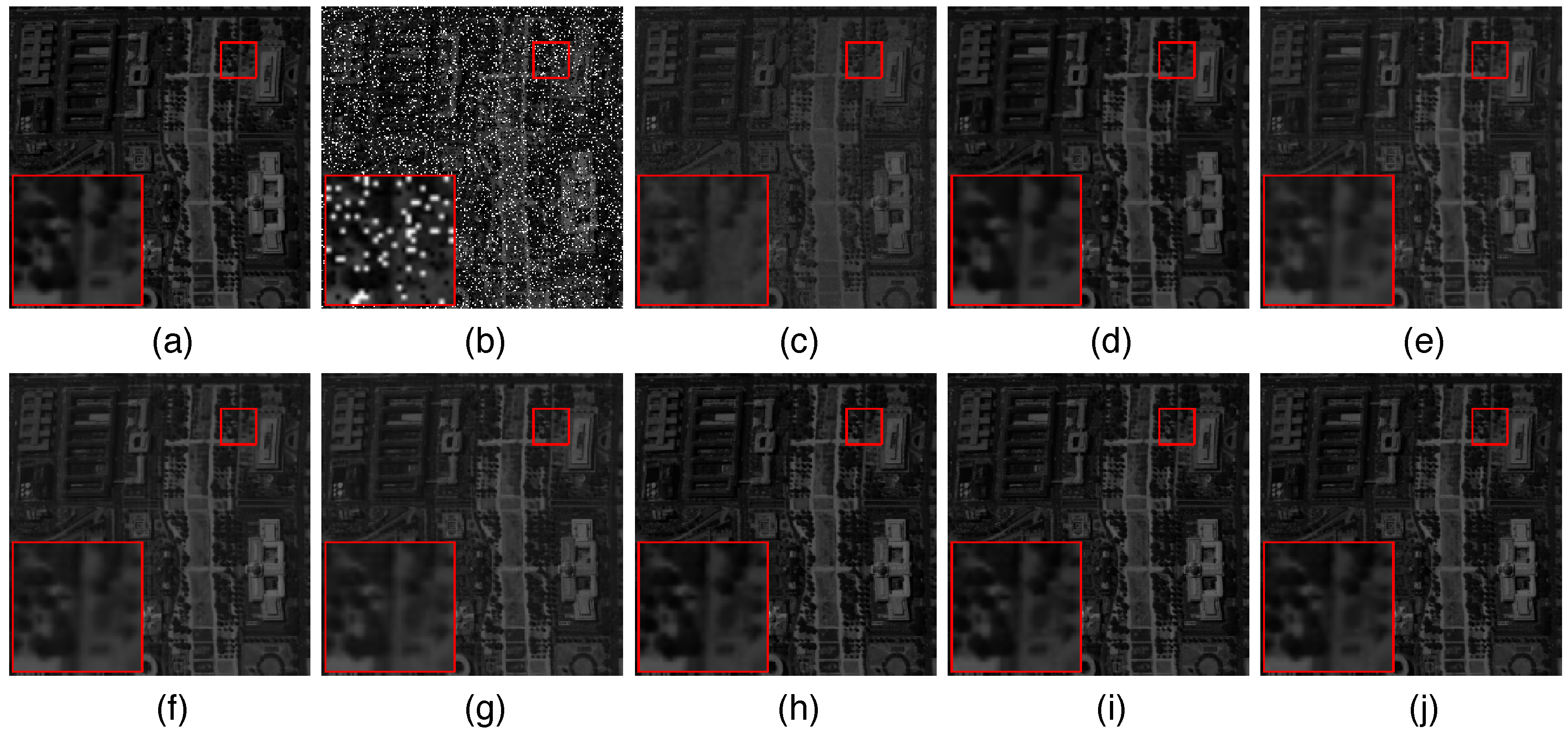
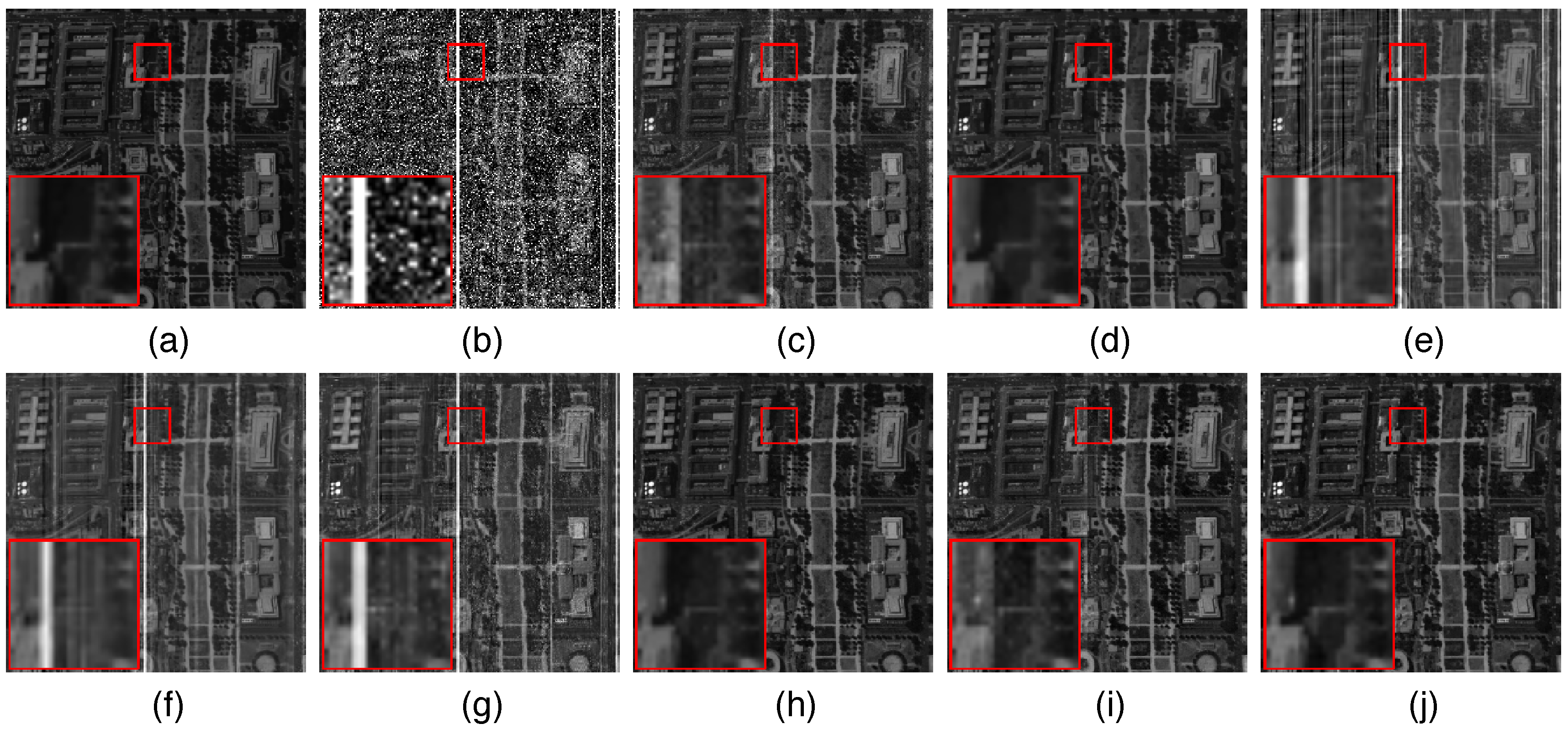
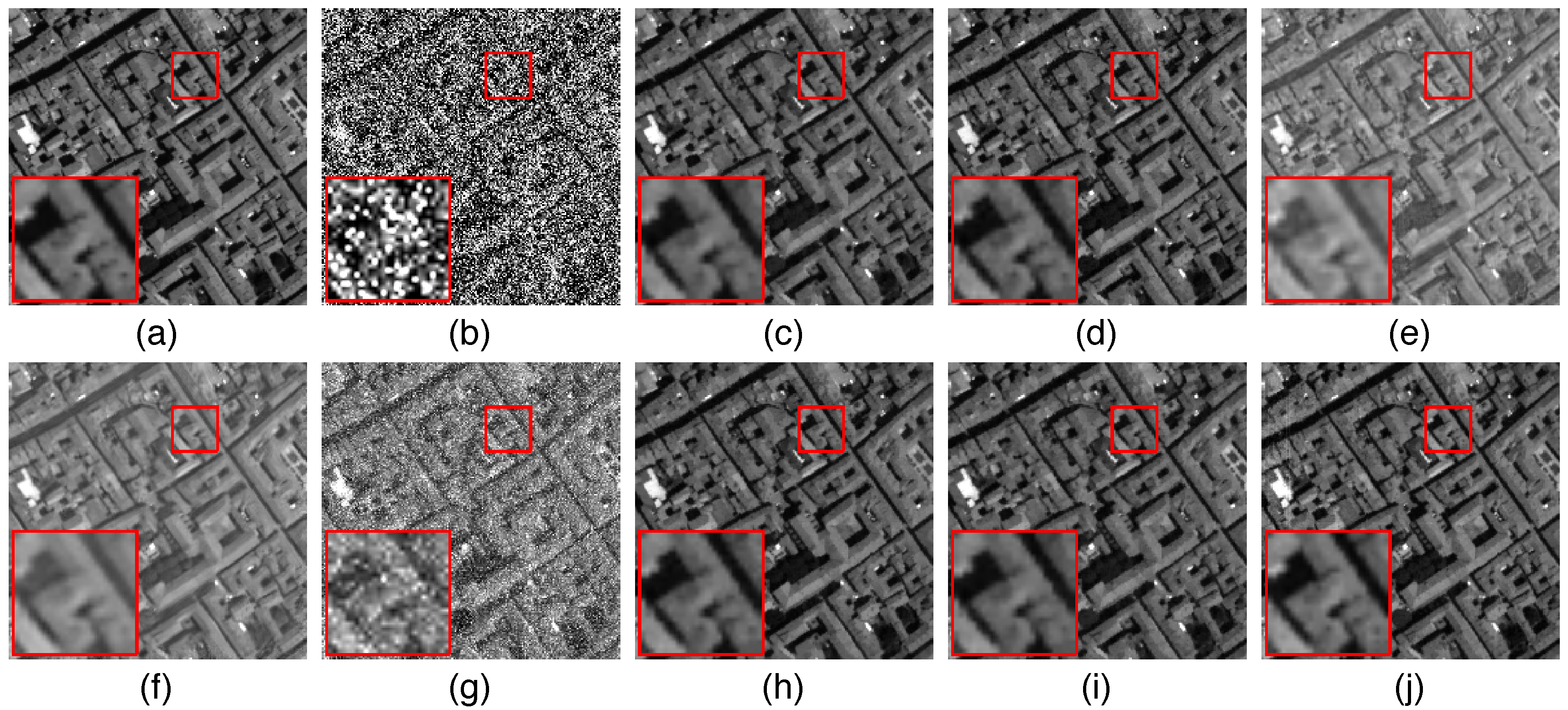
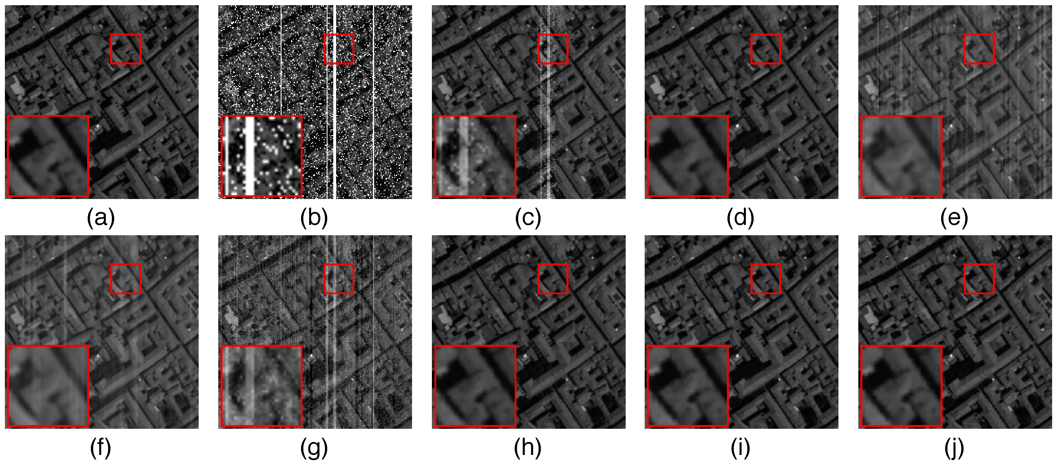
(2) Visual comparison: To compare the overall performance, two representative cases 3 and 4 are selected for visual inspection. Figure 3 and Figure 4 present the bands 159 and 52 obtained by different methods of Washington DC Mall under these two cases, respectively. Similarly, the restoration performances of the bands 21 and 41 of Pavia city center are shown in Figure 5 and Figure 6.

It can be evident that the original images suffer great contaminations in both cases as presented in Figure 3b–Figure 6b. In addition, the magnified subregion of each subfigure is given for a more detailed comparison. Figure 3 and Figure 5 display the performance of all competitors acting on images with mixtures of Gaussian and impulse noises. From Figure 3, we can observe that all competing methods can remove the great mass of noise. Among them, LRMR and FastHyDe come up several image distortion and over-smoothness. In addition, in comparison with the original image, LRTV, GLF, and NM-meet both smooth the image details to an extent. However, taking Figure 5g as an instance, it is obvious that some noise still remains in the restored image. In the meantime, different degrees of blurring can still be observed in the demarcated windows of Figure 5c–f. SMTVSF leads to a more faithful recovery (Figure 3 and Figure 5j) of the ground truth (Figure 3 and Figure 5a). Moreover, LLRGTV and LLRMTV can also successfully remove this mixed noise from the damaged band and preserve details as we expected. This further demonstrates the advantage of the TV-regularization in noise removal.

Figure 4 and Figure 6 display the performance of all competitors acting on images corrupted by the mixture of Gaussian noise, impulse noise, and deadlines. From Figure 4, it is easy to observe that FastHyDe, GLF, and NM-meet cannot completely remove this complex mixture noise, which contain some evident deadlines and introduce some stripe-like artifacts as shown in Figure 4e–g. LRMR obtains better results than the above three methods, but cannot thoroughly remove the deadlines. LRTV yields minor distortion compared with LRMR but blurs many details compared with the original clean image. In the meantime, a similar observation also appears in Figure 6. For LLRMTV, the deadlines are removed completely, but some residual noise is still nonnegligible, as can be seen in the zoom-in view of Figure 4i. In comparison, the proposed SMTVSF obtains the best visual quality and retains the essential edge structures. In addition, the LLRGTV method also has comparable performance, which is consistent with the following quantitative comparison.

(3) Quantitative comparison: Three objective quality metrics, i.e., peak-signal-to-noise ratio (PSNR), structural similarity index measurement (SSIM), and erreur relative globale adimensionnelle de synthese (ERGAS) are used in our study to evaluate the restoration accuracy. The smaller ERGAS, the larger mean PSNR (MPSNR), and mean SSIM (MSSIM), the closer the reference one.

For each noise setting of both simulated datasets,

Table 1. Quantitative assessment results obtained by different methods for simulated datasets.

Data	Noise Case	Metrics	Noisy	LRMR	LRTV	FastHyDe	GLF	NM-Meet	LLRGTV	LLRMTV	STVSF	SMTVSF
WDC	Case 1	MPSNR(dB)	26.02	39.04	38.27	40.54	40.82	39.90	40.51	39.93	40.22	41.43
		MSSIM	0.6929	0.9774	0.9758	0.9859	0.9878	0.9824	0.9826	0.9865	0.9850	0.9886
		ERGAS	194.29	42.63	46.71	37.08	36.18	40.65	35.93	40.66	38.24	33.86
	Case 2	MPSNR(dB)	15.86	34.61	34.68	30.41	30.54	29.03	35.85	35.63	34.46	36.27
		MSSIM	0.2869	0.9427	0.9430	0.9148	0.9163	0.8440	0.9531	0.9416	0.9421	0.9552
		ERGAS	632.75	69.58	69.22	128.60	128.34	149.90	60.21	69.44	70.81	65.91
	Case 3	MPSNR(dB)	14.16	33.53	34.81	27.00	27.53	26.80	36.85	36.31	35.50	37.20
		MSSIM	0.2335	0.9360	0.9509	0.8646	0.8797	0.8545	0.9606	0.9557	0.9531	0.9731
		ERGAS	843.87	89.40	74.11	218.27	214.35	227.83	63.91	62.44	68.79	48.67
	Case 4	MPSNR(dB)	13.87	33.38	34.41	26.11	26.56	26.05	34.81	35.09	33.73	35.58
		MSSIM	0.2285	0.9356	0.9447	0.8416	0.8579	8432	0.9505	0.9487	0.9300	0.9550
		ERGAS	856.52	99.61	79.69	244.56	236.70	238.96	140.05	85.05	183.90	74.31
		Time(Seconds)		240	103	14	807	95	672	727	18	44
Pavia	Case 1	MPSNR(dB)	26.02	38.49	38.96	40.82	41.58	39.02	39.27	39.10	40.21	41.42
		MSSIM	0.7209	0.9758	0.9775	0.9864	0.9886	0.9787	0.9795	0.9798	0.9844	0.9898
		ERGAS	184.54	44.89	43.44	33.92	31.01	42.78	40.90	40.15	36.25	30.28
	Case 2	MPSNR(dB)	15.86	33.20	34.62	29.89	29.95	26.94	34.14	34.33	34.10	35.03
		MSSIM	0.2858	0.9319	0.9426	0.9084	0.9104	0.7618	0.9388	0.9454	0.9297	0.9595
		ERGAS	596.67	81.63	73.85	119.68	117.78	187.20	73.48	71.66	77.50	69.23
	Case 3	MPSNR(dB)	13.99	32.46	33.87	26.09	26.70	24.65	34.39	34.85	33.90	34.77
		MSSIM	0.2200	0.9202	0.9365	0.8462	0.8715	0.7549	0.9478	0.9441	0.9357	0.9458
		ERGAS	796.17	99.36	101.87	200.54	189.66	269.95	78.56	82.76	81.32	68.17
	Case 4	MPSNR(dB)	13.80	31.21	33.88	24.75	25.52	24.30	34.16	34.22	33.37	34.56
		MSSIM	0.2371	0.9158	0.9276	0.7880	0.8393	0.7595	0.9599	0.9537	0.9584	0.9634
		ERGAS	824.19	140.04	155.72	251.02	236.27	284.28	82.01	86.12	85.50	74.55
		Time(Seconds)		67	21	8	474	52	33	115	4	22

lists the assessment results by the competing denoising methods, with the best results labeled in bold. These assessment values have great consistency with the visual effects, which manifest the superiority of the proposed method once again. In general, NM-meet shows worse denoising performance under complex mixed noise. Another observation is that FastHyDe and GLF can achieve comparable better performance in pure Gaussian noise cases, while, with the intensity of stripes and impulse noises increasing, the inferiority of the above-mentioned three methods is evident. LLRMTV and LLRGTV produce similar measurements. However, LLRMTV takes much more runtime since it introduces a new nonconvex regularizer. Meanwhile, we can observe that the proposed method is more competitive than LRMR, LRTV, and LLRGTV in complex mixed noise. This phenomenon validates the advantage of both subspace representation and nonconvex regularization for HSI restoration. Interestingly, the efficiency of our approach is only second to FastHyDe, but it outperforms all the competitors in qualitative metrics. In addition, we also report the corresponding quality metrics of the STVSF model, which can be directly considered as a combination of standard TV constraint and sparse representation. As seen, the performance of STVSF is relatively lower than SMTVSF. It once again verifies the effectiveness of the nonconvex regularization.

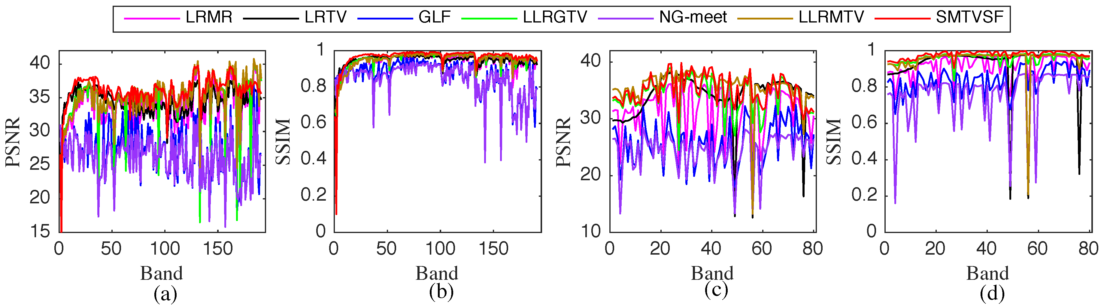
(4) Qualitative Comparison: Furthermore, the PSNR and SSIM measurements across all bands with different restoration algorithms of both datasets on case 4 are plotted in Figure 7. Note that GLF performs slightly better than FastHyDe. For simplicity, we do not show the visual restoration results of FastHyDe. From Figure 7a,b, it can be seen that SMTVSF obtains the higher PSNR and SSIM values on almost all bands of the Washington DC Mall data. For Pavia city center data, we obtain an average optimum in all channels as shown in Figure 7c,d.

4.2. Real Experiments

Here, we chose two real noisy HSI data to test the practicability of the proposed method, i.e., the Airborne Visible/Infrared Imaging Spectrometer (AVIRIS) Indian Pines dataset and the Hyperspectral Digital Imagery Collection Experiment (HYDICE) urban dataset. Similar to the synthetic experiments, we use default parameters or fine-tuned parameters to implement other competing methods, and the whole HSIs are also scaled to the interval [0, 1]. Since the subspace dimension of the real dataset needs to be predefined, the HySime algorithm [48] is adopted to estimate it.

(1) AVIRIS Indian Pines Dataset: We apply the proposed method to the AVIRIS Indian Pines data set [56]. This is an image with a size of $145\times 145\times 220$ and some bands are severely contaminated by Gaussian noise, salt and pepper, and unknown noise. The subspace dimension of this image is set to 25, which is generated by the HySime algorithm.

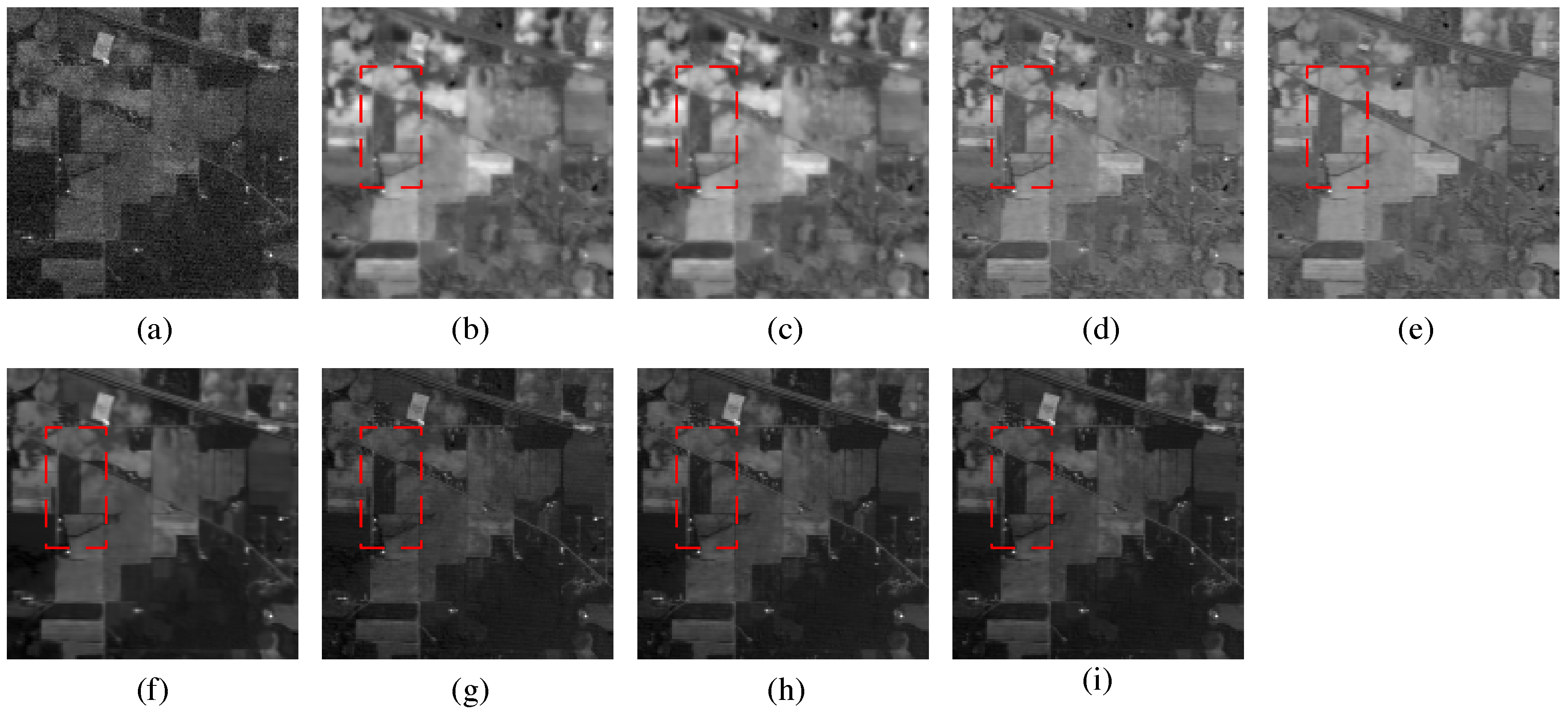
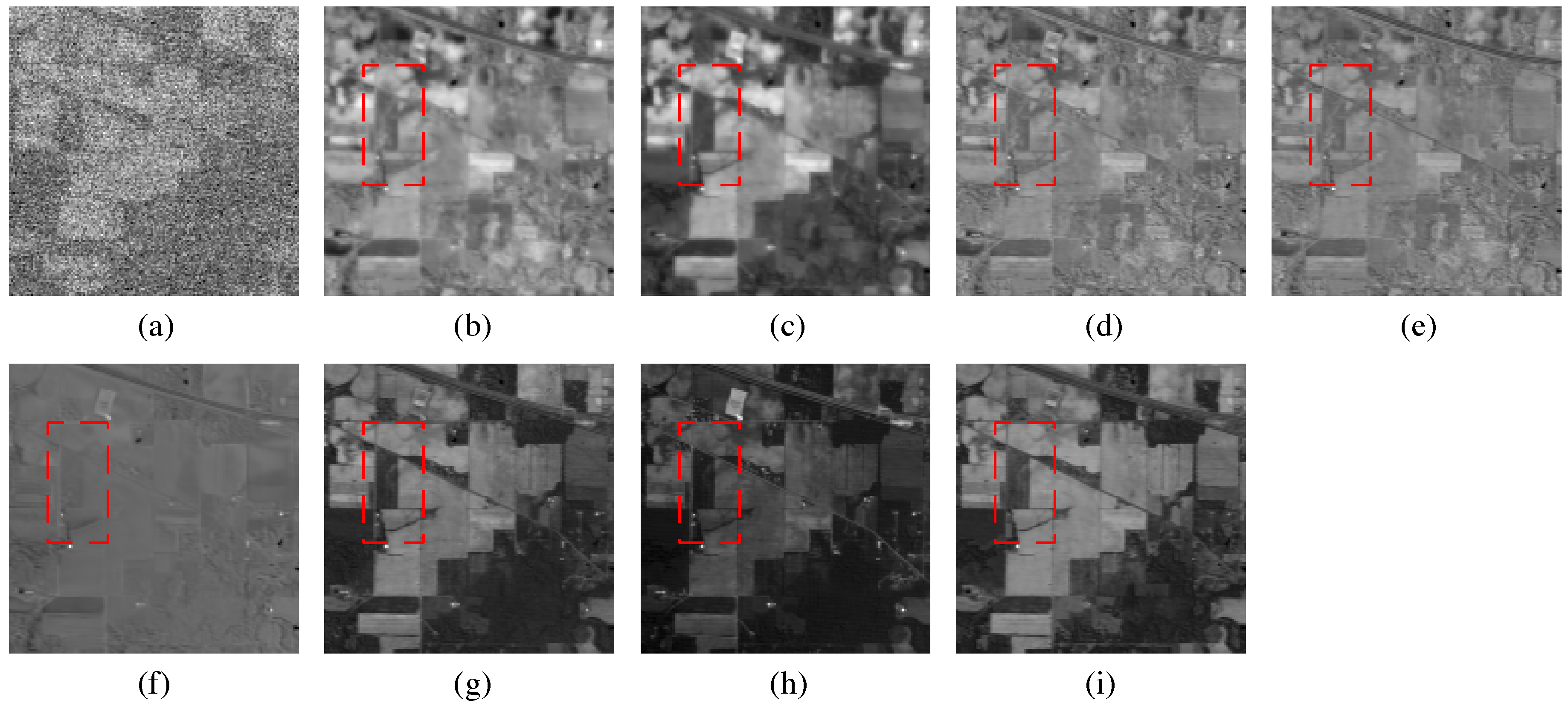
A visual comparison of bands 3 and 219 for all competing methods are given in Figure 8 and Figure 9, respectively. From Figure 8a, we can see that this band is degraded by Gaussian noise and sparse corruptions. LRMR and LRTV perform unsatisfactorily in the restoration. FastHyDe and GLF can obviously improve the spatial resolution, but some edges are not clearly differentiated, as the red dashed boxes shown in Figure 8d,e. NM-meet can moderately preserve the details, but when image is heavily contaminated by mixed noise, it loses its practicality, as presented in Figure 9f. The underlying reason is that NGmeet aims to eliminate Gaussian noise. Obviously, when the noise level increases, LRMR, LRTV, FastHyDe, and GLF result in a less competitive performance (see Figure 8 and Figure 9b–e). The results of LLRMTV, LLRGTV, and SMTVSF have relatively less noise. We can also see that the restored HSI of LLRGTV maintains some horizontal stripes, as presented in Figure 8g. Meanwhile, SMTVSF introduces some artifacts, as presented in Figure 9i. Comparatively, for this data set, LLRMTV can wipe out the noise efficiently and deliver a better visual appearance.

(2) HYDICE Urban Dataset: The urban area HYDICE dataset [57] is provided by Chen et al. [21] and seriously polluted by the atmosphere, stripes and dead lines. The size of the scene is $307\times 307\times 210$, and we feed a subimage of $200\times 200\times 210$ into the denoising algorithms. In this set of experiments, the value of the subspace dimension is set to 4.

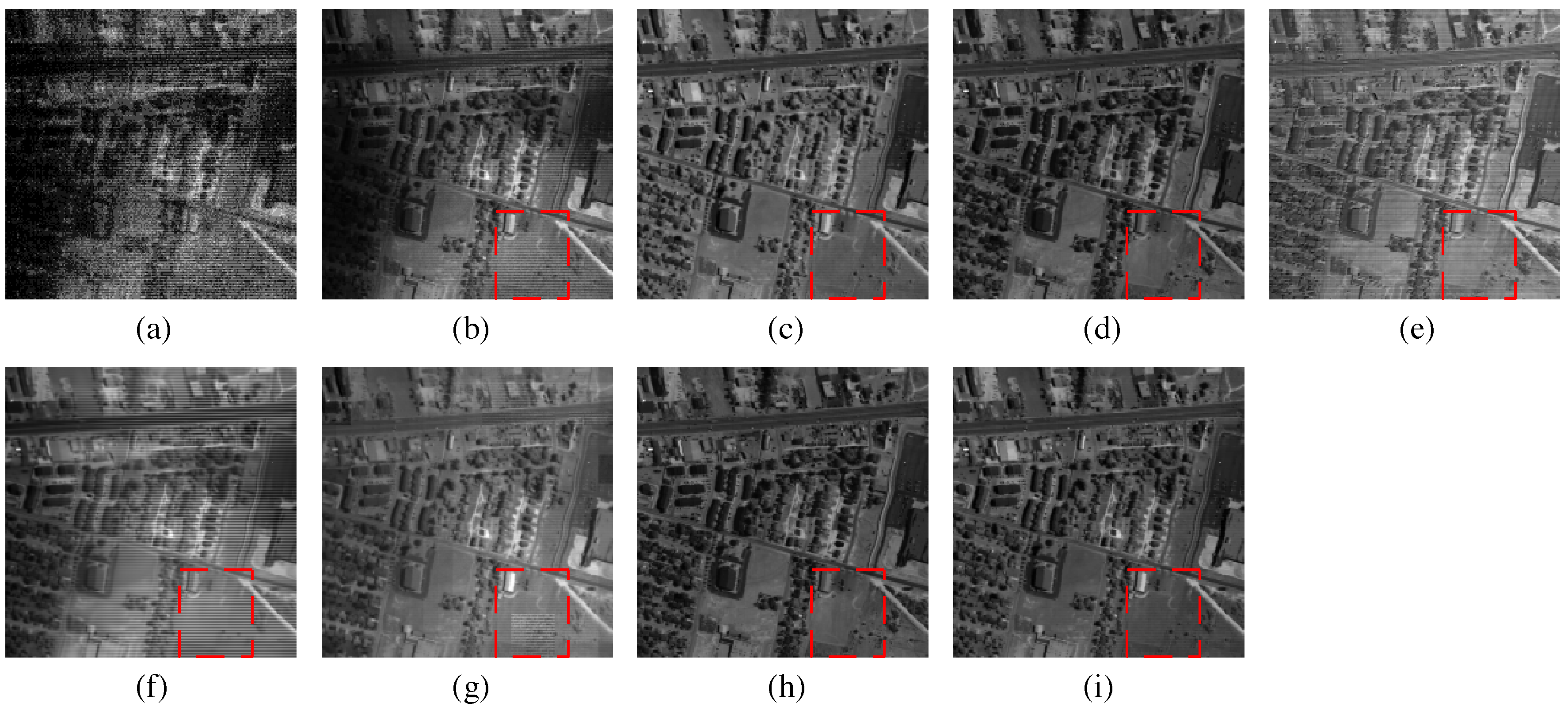
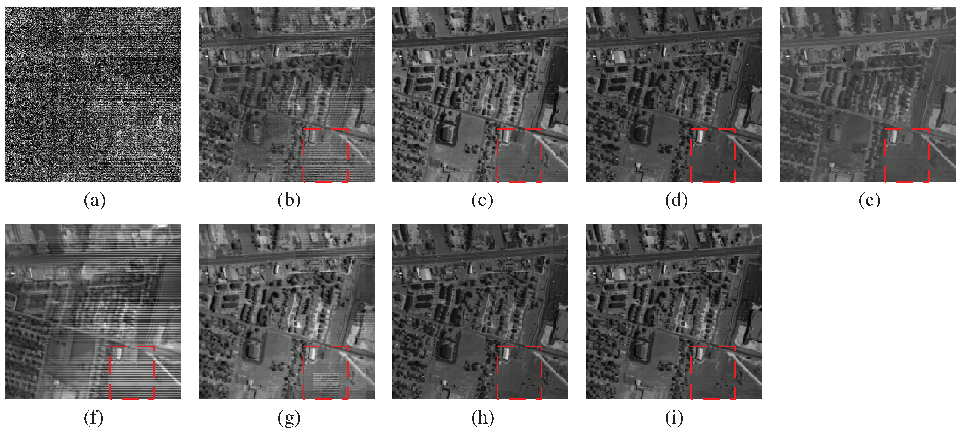
We also select two typical bands to depict the denoising performance of different methods. Figure 10 shows the band 139 before and after denoising, while Figure 11 provides a visual comparison of the band 208. It is not hard to see that LRMR, GLF, and NM-meet cannot effectively remove the stripes, and also introduce artifacts into the final results. LLRGTV can remove random noise, but it still shows stripes remaining as presented in Figure 10g and Figure 11g. This is because the stripes and deadlines in this scene exist in the same location in some adjacent bands and the low-rank based method treats the structured sparse noise as a clean image component. LRTV and FastHyDe perform comparatively better in destriping. However, LRTV would over-smooth the details. LLRMTV can remove this mixed noise and the corresponding edges are relatively clear as shown in Figure 10h and Figure 11h. Benefitting from the ‘Moreau-enhanced’ Total Variation and sparse representation regularizations, the proposed SMTVSF method can eliminate complicated noise and finely recover the details hiding under the polluted HSI.

Figure 12 shows a more intuitive verification with respect to the horizontal mean profiles of the band 139 before and after applying all of the compared techniques. The evident fluctuations in Figure 12a indicate that severely stripes are located in the image. From the restored curves, it can be observed that LRMR, LRTV, GLF, and NM-meet fail to keep a right curve tendency. By contrast, FastHyDe generates noticeable distortion. LLRMTV can obtain a relatively smoother curve than SMTVSF, which agrees with the visual results drawn in Figure 10. Our comprehensive experiments show that SMTVSF can achieve some competitive performance compared with other popular methods (e.g., LLRGTV), which indicates the effectiveness of SMTVSF for HSI restoration.

(3) Running Time:

Table 2. Running Time (in seconds) of all competitors on two real HSI datasets

HSI Data	LRMR	LRTV	FastHyDe	GLF	NM-Meet	LLRGTV	LLRMTV	SMTVSF
Indian Pines	74	28	6	273	25	220	76	20
HYDICE Urban	149	51	10	475	56	463	108	24

compares the processing time of all methods on two real-world HSIs. From the table, we can conclude that FastHyDe is the fastest method and our method is slightly slower than it. However, we provide better restored results than FastHyDe. This is mainly because our algorithm requires the use of a non-separable non-convex TV denoising penalty to converge to the final solution.

4.3. Parameter Sensitivity

Several critical parameters in the restoration model (13) need to be carefully identified, including regularization parameters ${\lambda }_1$ and ${\lambda }_2$, subspace dimension k, and non-convex control parameter $\alpha$. In the following, we first present the optimal values of these parameter settings and then display the convergence curve of our method. Please note that all the results are based on simulated Washington DC Mall case 4.

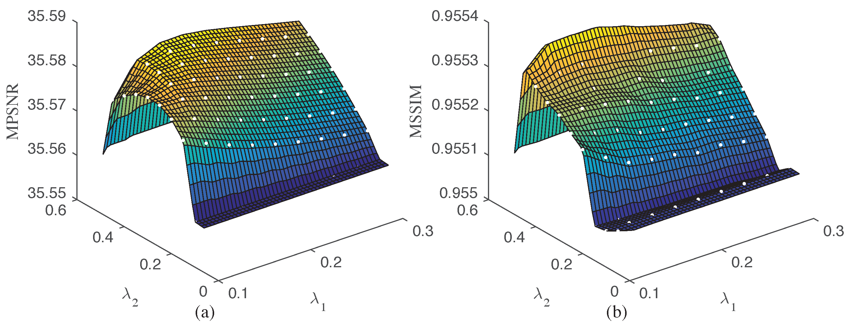
(1) Parameter ${\lambda }_1$ and ${\lambda }_2$: We tune ${\lambda }_1$ from 0.05 to 0.5 with an interval of 0.05 and ${\lambda }_2$ from 0.1 to 0.3 with an interval of 0.025, respectively. Figure 13 shows the curves of the MPSNR and MSSIM values with changing ${\lambda }_1$ and ${\lambda }_2$. Clearly, the proposed method performs appealing results when ${\lambda }_2$ = 0.45 and ${\lambda }_1$ lied in the range of [0.125, 0.275]. Therefore, we empirically set ${\lambda }_1$ = 0.2 and ${\lambda }_2$ = 0.45 in all experiments.

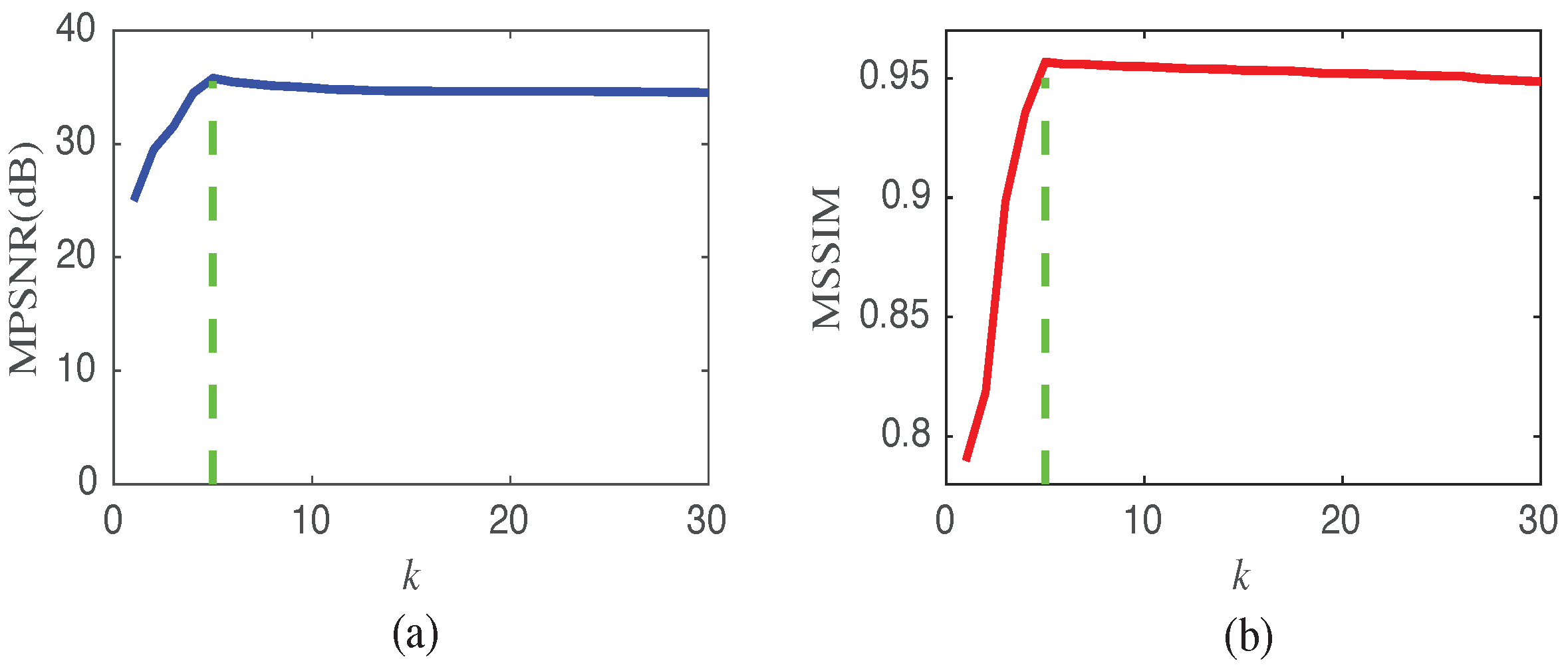
(2) Subspace Dimension k: Subspace dimension k has an inherent relationship with the size of the projection matrix. A detailed construction of the subspace A is listed in Appendix B. Figure 14 presents the influence of parameters k from 1 to 30 on the denoising performance in terms of MPSNR and MSSIM values. As can be observed, the two objective metrics achieve the optimal performance when k is set to 5. However, this is different from the evaluation result k = 4 of the HySime algorithm [48], mainly because it only considers Gaussian noise. In our experiments, the subspace dimension needs to be assigned manually according to the data itself.

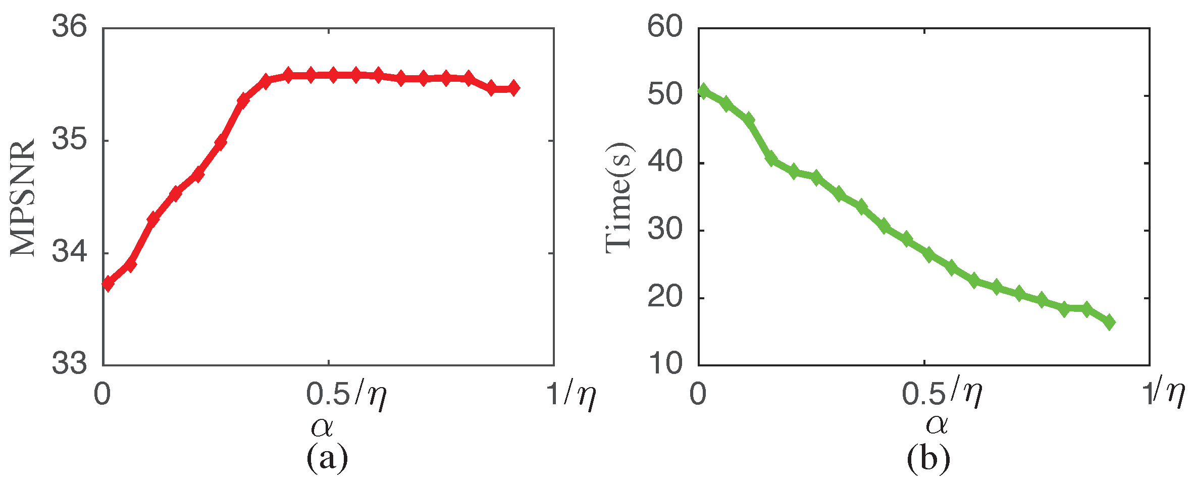
(3) Parameter α: $\alpha$ is the non-convex control parameter, which directly influences the solution of (15). Empirically fixing $\eta$ as $0.125\times \sqrt{MN}$, we vary $\alpha$ within the scope of (0, 1/$\eta$) and show the performance in Figure 15. Intuitively, when $\alpha$ falls within the range of [0.4, 0.95]/$\eta$, the MPSNR values of the proposed method are relatively stable. When $\alpha$ increases, the time consumption decreases sharply as model (11) will be strongly convex and have a unique minimizer (see Figure 15b). Taking both denoising performance and computational complexity into consideration, $\alpha$ is set to 0.7/$\eta$ in all our experiments.

(4) Convergence Analysis: In Figure 16, we display the changes of the objective function and MPSNR values with the iteration number. Here, we can easily observe that, with the increment of iteration number, these values increase rapidly. After the number is greater than 20, the performance is relatively stable, indicating that our method can be successfully converged.

5. Conclusions

In this paper, we propose a subspace-based method, namely SMTVSF, for HSI denoising. Our SMTVSF model integrates the spectral low-rank property and spatial sparsity into a general fomulation. Specifically, these two terms are explored by subspace representation and representation coefficients denoising, respectively. Our technological process starts by decomposing an HSI into two submatrices with lower dimensions, thereby reducing the computational burden. Subsequently, for each subspace representation image, a Moreau-enhanced Total Variation denoising model is utilized to promote the spatial piecewise smoothness and consistency of the HSI. In addition, ${\ell }_{2,1}$-norm regularization is further embedded to distinguish the stripe component. Extensive experiments verify that, compared with other competitors, our method can both achieve a better accuracy performance and obtain an acceptable running time. Inspired the spatial-spectral TV regularization idea, in our future work, we plan to develop a 3D Moreau-enhanced TV denoising model used in HSI denoising for deeper feature learning both spatially and spectrally.

References

- Goetz, A.F.H. Three decades of hyperspectral remote sensing of the earth: A personal view. Remote Sens. Environ. 2009, 113, S5–S16. [Google Scholar] [CrossRef]
- Willett, R.M.; Duarte, M.F.; Davenport, M.A.; Baraniuk, R.G. Sparsity and structure in hyperspectral imaging: Sensing, reconstruction, and target detection. IEEE Signal Process. Mag. 2014, 31, 116–126. [Google Scholar] [CrossRef] [Green Version]
- Peng, Y.; Meng, D.; Xu, Z.; Gao, C.; Yang, Y.; Zhang, B. Decomposable nonlocal tensor dictionary learning for multispectral image denoising. In Proceedings of the IEEE Conference Computer Vision Pattern Recognit, Columbus, OH, USA, 23–28 June 2014; pp. 2949–2956. [Google Scholar]
- Wu, Z.; Shi, L.; Li, J.; Wang, Q.; Sun, L.; Wei, Z.; Plaza, J.; Plaza, A. GPU parallel implementation of spatially adaptive hyperspectral image classification. IEEE J. Sel. Top. Appl. Earth Obs. Remote Sens. 2018, 11, 1131–1143. [Google Scholar] [CrossRef]
- Feng, R.; Wang, L.; Zhong, Y. Joint Local Block Grouping with Noise-Adjusted Principal Component Analysis for Hyperspectral Remote-Sensing Imagery Sparse Unmixing. Remote Sens. 2019, 11, 1223. [Google Scholar] [CrossRef] [Green Version]
- Sun, L.; Wu, Z.; Xiao, L.; Liu, J.; Wei, Z.; Dang, F. A novel ℓ1/2 sparse regression method for hyperspectral unmixing. Int. J. Remote Sens. 2013, 34, 6983–7001. [Google Scholar] [CrossRef]
- Xu, Y.; Wu, Z.; Li, J.; Plaza, A.; Wei, Z. Anomaly detection in hyperspectral images based on low-rank and sparse representation. IEEE Trans. Geosci. Remote Sens. 2016, 54, 1990–2000. [Google Scholar] [CrossRef]
- Zhang, L.; Zhang, Y.; Yan, H.; Gao, Y.; Wei, W. Salient object detection in hyperspectral imagery using multi-scale spectral-spatial gradient. Neurocomputing 2018, 291, 215–225. [Google Scholar] [CrossRef]
- Elad, M.; Aharon, M. Image denoising via sparse and redundant representations over learned dictionaries. IEEE Trans. Image Process. 2006, 15, 3736–3745. [Google Scholar] [CrossRef]
- Dabov, K.; Foi, A.; Katkovnik, V.; Egiazarian, K. Image denoising by sparse 3D transform-domain collaborative filtering. IEEE Trans. Image Process. 2007, 16, 2080–2095. [Google Scholar] [CrossRef]
- Dong, W.; Zhang, L.; Shi, G.; Li, X. Nonlocally centralized sparse representation for image restoration. IEEE Trans. Image Process. 2013, 22, 1620–1630. [Google Scholar] [CrossRef] [Green Version]
- Yuan, Q.; Zhang, L.; Shen, H. Hyperspectral image denoising employing a spectral-spatial adaptive total variation model. IEEE Trans. Geosci. Remote Sens. 2012, 50, 3660–3677. [Google Scholar] [CrossRef]
- Zhang, H. Hyperspectral image denoising with cubic total variation model. SPRS Ann. Photogramm. Remote Sens. Spat. Inf. Sci. 2012, 7, 95–98. [Google Scholar] [CrossRef] [Green Version]
- Qian, Y.; Ye, M. Hyperspectral imagery restoration using nonlocal spectral-spatial structured sparse representation with noise estimation. IEEE J. Sel. Top. Appl. Earth Obs. Remote Sens. 2013, 6, 499–515. [Google Scholar] [CrossRef]
- Letexier, D.; Bourennane, S. Multidimensional wiener filtering using fourth order statistics of hyperspectral images. In Proceedings of the 2008 IEEE International Conference on Acoustics, Speech and Signal Processing, Las Vegas, NV, USA, 31 March–4 April 2008; pp. 917–920. [Google Scholar]
- Maggioni, M.; Katkovnik, V.; Egiazarian, K.; Foi, A. Nonlocal transform-domain filter for volumetric data denoising and reconstruction. IEEE Trans. Image Process. 2013, 22, 119–133. [Google Scholar] [CrossRef]
- Candès, E.J.; Li, X.; Ma, Y.; Wright, J. Robust principal component analysis? J. ACM 2011, 58, 1–37. [Google Scholar] [CrossRef]
- Zhang, H.; He, W.; Zhang, L.; Shen, H.; Yuan, Q. Hyperspectral image restoration using low-rank matrix recovery. IEEE Trans. Geosci. Remote Sens. 2014, 52, 4729–4743. [Google Scholar] [CrossRef]
- He, W.; Zhang, H.; Zhang, L.; Shen, H. Hyperspectral Image Denoising via Noise-Adjusted Iterative Low-Rank Matrix Approximation. IEEE J. Sel. Top. Appl. Earth Obs. Remote Sens. 2015, 8, 3050–3061. [Google Scholar] [CrossRef]
- Xie, Y.; Qu, Y.; Tao, D.; Wu, W.; Yuan, Q.; Zhang, W. Hyperspectral image restoration via iteratively regularized weighted schatten p-norm minimization. IEEE Trans. Geosci. Remote Sens. 2016, 54, 4642–4659. [Google Scholar] [CrossRef]
- Chen, Y.; Guo, Y.; Wang, Y.; Wang, D.; Peng, C.; He, G. Denoising of hyperspectral images using nonconvex low rank matrix approximation. IEEE Trans. Geosci. Remote Sens. 2017, 55, 5366–5380. [Google Scholar] [CrossRef]
- Sun, L.; Jeon, B.; Zheng, Y.; Wu, Z. Hyperspectral image restoration using low-rank representation on spectral difference image. IEEE Geosci. Remote Sens. Lett. 2017, 14, 1151–1155. [Google Scholar] [CrossRef]
- Song, X.; Wu, L.; Hao, H.; Xu, W. Hyperspectral Image Denoising Based on Spectral Dictionary Learning and Sparse Coding. Electronics 2019, 8, 86. [Google Scholar] [CrossRef] [Green Version]
- Fan, F.; Ma, Y.; Li, C.; Mei, X.; Huang, J.; Ma, J. Hyperspectral image denoising with superpixel segmentation and low-rank representation. Inf. Sci. 2017, 397/398, 48–68. [Google Scholar] [CrossRef]
- Zhu, R.; Dong, M.; Xue, J.H. Spectral Nonlocal Restoration of Hyperspectral Images With Low-Rank Property. IEEE J. Sel. Top. Appl. Earth Obs. Remote Sens. 2015, 8, 3062–3067. [Google Scholar]
- Guo, X.; Huang, X.; Zhang, L.; Zhang, L. Hyperspectral image noise reduction based on rank-1 tensor decomposition. Int. Soc. Photogramm. Remote Sens. J. Photogramm. Remote Sens. 2013, 83, 50–63. [Google Scholar] [CrossRef]
- Xie, Q.; Zhao, Q.; Meng, D.; Xu, Z.; Gu, S.; Zuo, W.; Zhang, L. Multispectral Images Denoising by Intrinsic Tensor Sparsity Regularization. In Proceedings of the IEEE Conference on Computer Vision and Pattern Recognition, Las Vegas, NV, USA, 27–30 June 2016; pp. 1692–1700. [Google Scholar]
- Wu, Z.; Wang, Q.; Jin, J.; Shen, Y. Structure tensor total variation-regularized weighted nuclear norm minimization for hyperspectral image mixed denoising. Signal Process. 2017, 131, 202–219. [Google Scholar] [CrossRef]
- Xue, J.; Zhao, Y.; Liao, W.; Chan, J.C.-W. Nonlocal Low-Rank Regularized Tensor Decomposition for Hyperspectral Image Denoising. IEEE Trans. Geosci. Remote Sens. 2019, 57, 5174–5189. [Google Scholar] [CrossRef]
- Kong, X.; Zhao, Y.; Xue, J.; Chan, J.C.-W. Hyperspectral Image Denoising Using Global Weighted Tensor Norm Minimum and Nonlocal Low-Rank Approximation. Remote Sens. 2019, 11, 2281. [Google Scholar] [CrossRef] [Green Version]
- He, W.; Zhang, H.; Zhang, L.; Shen, H. Total-variation-regularized low-rank matrix factorization for hyperspectral imagerestoration. IEEE Trans. Geosci. Remote Sens. 2016, 54, 178–188. [Google Scholar] [CrossRef]
- Rudin, L.I.; Osher, S.; Fatemi, E. Nonlinear total variation based noise removal algorithms. Phys. D Nonlinear Phenom. 1992, 60, 259–268. [Google Scholar] [CrossRef]
- Wu, Z.; Wang, Q.; Wu, Z.; Shen, Y. Total variation-regularized weighted nuclear norm minimization for hyperspectral image mixed denoising. J. Electron. Imag. 2016, 25, 1–21. [Google Scholar] [CrossRef]
- Gu, S.; Zhang, L.; Zuo, W.; Feng, X. Weighted Nuclear Norm Minimization with Application to Image Denoising. In Proceedings of the IEEE Conference on Computer Vision and Pattern Recognition, Columbus, OH, USA, 23–28 June 2014; pp. 2862–2869. [Google Scholar]
- Sun, L.; Zhan, T.; Wu, Z.; Jeon, B. A Novel 3D Anisotropic Total Variation Regularized Low Rank Method for Hyperspectral Image Mixed Denoising. ISPRS Int. J. Geo-Inf. 2018, 7, 412. [Google Scholar] [CrossRef] [Green Version]
- Aggarwal, H.K.; Majumdar, A. Hyperspectral Image Denoising Using Spatio-Spectral Total Variation. IEEE Geosci. Remote Sens. Lett. 2016, 13, 442–446. [Google Scholar] [CrossRef]
- He, W.; Zhang, H.; Shen, H.; Zhang, L. Hyperspectral Image Denoising Using Local Low-Rank Matrix Recovery and Global Spatial–Spectral Total Variation. IEEE J. Sel. Top. Appl. Earth Obs. Remote Sens. 2018, 11, 713–729. [Google Scholar] [CrossRef]
- Li, Q.; Zhong, R.; Wang, Y. A Method for the Destriping of an Orbita Hyperspectral Image with Adaptive Moment Matching and Unidirectional Total Variation. Remote Sens. 2019, 11, 2098. [Google Scholar] [CrossRef] [Green Version]
- Lefkimmiatis, S.; Roussos, A.; Maragos, P.; Unser, M. Structure tensor total variation. SIAM J. Imaging Sci. 2015, 8, 1090–1122. [Google Scholar] [CrossRef]
- Zhuang, L.; Bioucas-Dias, J.M. Fast Hyperspectral image Denoising based on low rank and sparse representations. In Proceedings of the 2016 IEEE International Geoscience and Remote Sensing Symposium (IGARSS), Beijing, China, 10–15 July 2016; pp. 1847–1850. [Google Scholar]
- Zhuang, L.; Bioucas-Dias, J.M. Hyperspectral image denoising based on global and non-local low-rank factorizations. In Proceedings of the 2017 IEEE International Conference on Image Processing (ICIP), Beijing, China, 17–20 September 2017; pp. 1900–1904. [Google Scholar]
- He, W.; Yao, Q.; Li, C.; Yokoya, N.; Zhao, Q. Non-local Meets Global: An Integrated Paradigm for Hyperspectral Denoising. arXiv 2018, arXiv:1812.04243. [Google Scholar]
- Yang, Y.; Zheng, J.; Chen, S.; Zhang, M. Hyperspectral image restoration via local low-rank matrix recovery and Moreau-enhanced total variation. IEEE Geosci. Remote Sens. Lett. 2019. [Google Scholar] [CrossRef]
- Qian, Y.; Shen, Y.; Ye, M.; Wang, Q. 3D nonlocal means filter withnoise estimation for hyperspectral imagery denoising. In Proceedings of the 2012 IEEE International Geoscience and Remote Sensing Symposium, Munich, Germany, 22–27 July 2012; pp. 1345–1348. [Google Scholar]
- Xue, J.; Zhao, Y.; Liao, W.; Kong, S.G. Joint Spatial and Spectral Low-Rank Regularization for Hyperspectral Image Denoising. IEEE Trans. Geosci. Remote Sens. 2018, 56, 1940–1958. [Google Scholar] [CrossRef]
- Zhuang, L.; Bioucas-Dias, J.M. Fast hyperspectral image denoising and inpainting based on low-rank and sparse representations. IEEE J. Sel. Top. Appl. Earth Obs. Remote Sens. 2018, 11, 730–742. [Google Scholar] [CrossRef]
- Rasti, B.; Scheunders, P.; Ghamisi, P.; Licciardi, G.; Chanussot, J. Noise reduction in hyperspectral imagery: Overview and application. Remote Sens. 2018, 10, 482. [Google Scholar] [CrossRef] [Green Version]
- Bioucas-Dias, J.M.; Nascimento, J.M. Hyperspectral Subspace Identification. IEEE Trans. Geosci. Remote Sens. 2008, 46, 2435–2445. [Google Scholar] [CrossRef] [Green Version]
- Bauschke, H.H.; Combettes, P.L. Convex Analysis and Monotone Operator Theory in Hilbert Spaces; Springer: New York, NY, USA, 2011; pp. 561–575. [Google Scholar]
- Selesnick, I. Total Variation Denoising Via the Moreau Envelope. IEEE Signal Process. Lett. 2017, 24, 216–220. [Google Scholar] [CrossRef]
- He, W.; Zhang, H.; Zhang, L. Total variation regularized reweighted sparse nonnegative matrix factorization for hyperspectral unmixing. IEEE Trans. Geosci. Remote Sens. 2017, 55, 3909–3921. [Google Scholar] [CrossRef]
- Lin, Z.; Chen, M.; Ma, Y. The augmented lagrange multiplier method for exact recovery of corrupted low-rank matrices. arXiv 2010, arXiv:1009.5055. [Google Scholar]
- Yang, J.; Yin, W.; Zhang, Y.; Wang, Y. A Fast Algorithm for Edge-Preserving Variational Multichannel Image Restoration. SIAM J. Imaging Sci. 2009, 2, 569–592. [Google Scholar] [CrossRef]
- A Freeware Multispectral Image Data Analysis System. Available online: https://engineering.purdue.edu/~biehl/MultiSpec/hyperspectral.html (accessed on 30 December 2019).
- Hyperspectral Remote Sensing Scenes. Available online: http://www.ehu.es/ccwintco/index.php/Hyperspectral_Remote_Sensing_Scenes (accessed on 30 December 2019).
- AVIRIS Indian Pines Dataset. Available online: http://www.ehu.eus/ccwintco/index.php (accessed on 15 May 2019).
- HYDICE Urban Dataset. Available online: https://www.researchgate.net/publication/315725239_Code_of_NonLRMA (accessed on 15 May 2019).
- Combettes, P.L.; Pesquet, J.-C. Proximal splitting methods in signal processing. In Fixed-Point Algorithms for Inverse Problems in Science and Engineering; Bauschke, H.H., Burachik, R.S., Combettes, P.L., Elser, V., Luke, D.R., Wolkowicz, H., Eds.; Springer: New York, NY, USA, 2011; Volume 49, pp. 185–212. [Google Scholar]
- Cai, J.F.; Candès, E.J.; Shen, Z. A Singular Value Thresholding Algorithm for Matrix Completion. Soc. Ind. Appl. Math. J. Opt. 2008, 20, 1956–1982. [Google Scholar] [CrossRef]
Figure 1.
Comparison of the abundance image (after denoised) and the absolute error characteristic value between denoised and the reference. Top row: TV denoised results. Bottom row: MTV denoised results.
Figure 2.
Flowchart of the proposed SMTVSF denoising model.
Figure 3.
Denoised results of Washington DC dataset under case 3. (a) original band 159, (b) Noisy, (c) LRMR, (d) LRTV, (e) FastHyDe, (f) GLF, (g) NM-meet, (h) LLRGTV, (i) LLRMTV, (j) SMTVSF.
Figure 4.
Denoised results of Washington DC dataset under case 4. (a) original band 52, (b) Noisy, (c) LRMR, (d) LRTV, (e) FastHyDe, (f) GLF, (g) NM-meet, (h) LLRGTV, (i) LLRMTV, (j) SMTVSF.
Figure 5.
Denoised results of Pavia city center dataset under case 3. (a) original band 21, (b) Noisy, (c) LRMR, (d) LRTV, (e) FastHyDe, (f) GLF, (g) NM-meet, (h) LLRGTV, (i) LLRMTV, (j) SMTVSF.
Figure 6.
Denoised results of Pavia city center dataset under case 4. (a) original band 41, (b) Noisy, (c) LRMR, (d) LRTV, (e) FastHyDe, (f) GLF, (g) NM-meet, (h) LLRGTV, (i) LLRMTV, (j) SMTVSF.
Figure 7.
PSNR and SSIM measurements of all bands in case 4. (a,b) Washington DC Mall dataset, (c,d) Pavia city center dataset.
Figure 8.
Denoised images of all the competing approaches in Indian Pines data set. (a) original band 3, (b) LRMR, (c) LRTV, (d) FastHyDe, (e) GLF, (f) NM-meet, (g) LLRGTV, (h) LLRMTV, (i) SMTVSF.
Figure 9.
Denoised images of all the competing approaches in Indian Pines data set. (a) original band 219, (b) LRMR, (c) LRTV, (d) FastHyDe, (e) GLF, (f) NM-meet, (g) LLRGTV, (h) LLRMTV, (i) SMTVSF.
Figure 10.
Denoised images of all the competing approaches in Urban data set. (a) original band 139, (b) LRMR, (c) LRTV, (d) FastHyDe, (e) GLF, (f) NM-meet, (g) LLRGTV, (h) LLRMTV, (i) SMTVSF.
Figure 11.
Denoised images of all the competing approaches in Urban data set. (a) original band 208, (b) LRMR, (c) LRTV, (d) FastHyDe, (e) GLF, (f) NM-meet, (g) LLRGTV, (h) LLRMTV, (i) SMTVSF.
Figure 12.
Original and recovered horizontal mean profiles from the Urban HSI data. (a) original band 139, (b) LRMR, (c) LRTV, (d) FastHyDe, (e) GLF, (f) NM-meet, (g) LLRGTV, (h) LLRMTV, (i) SMTVSF.
Figure 13.
Restoration results with respect to parameters and . (a) MPSNR, (b) MSSIM.
Figure 14.
Restoration results under different values of subspace dimension k. (a) MPSNR, (b) MSSIM.
Figure 15.
Sensitivity analysis of . (a) MPSNR values, (b) time values.
Figure 16.
Convergence analysis with the iteration number. (a) objective function value, (b) MPSNR.