Developing Land Surface Directional Reflectance and Albedo Products from Geostationary GOES-R and Himawari Data: Theoretical Basis, Operational Implementation, and Validation

Abstract

The new generation of geostationary satellite sensors is producing an unprecedented amount of Earth observations with high temporal, spatial and spectral resolutions, which enable us to detect and assess abrupt surface changes. In this study, we developed the land surface directional reflectance and albedo products from Geostationary Operational Environment Satellite-R (GOES-R) Advanced Baseline Imager (ABI) data using a method that was prototyped with the Moderate Resolution Imaging Spectroradiometer (MODIS) data in a previous study, and was also tested with data from the Advanced Himawari Imager (AHI) onboard Himawari-8. Surface reflectance is usually retrieved through atmospheric correction that requires the input of aerosol optical depth (AOD). We first estimated AOD and the surface bidirectional reflectance factor (BRF) model parameters simultaneously based on an atmospheric radiative transfer formulation with surface anisotropy, and then calculated the “blue-sky” surface broadband albedo and directional reflectance. This algorithm was implemented operationally by the National Oceanic and Atmospheric Administration (NOAA) to generate the GOES-R land surface albedo product suite with a daily updated clear-sky satellite observation database. The “operational” land surface albedo estimation from ABI and AHI data was validated against ground measurements at the SURFRAD sites and OzFlux sites and compared with the existing satellite products, including MODIS, Visible infrared Imaging Radiometer (VIIRS), and Global Land Surface Satellites (GLASS) albedo products, where good agreement was found with bias values of −0.001 (ABI) and 0.020 (AHI) and root-mean-square-errors (RMSEs) less than 0.065 for the hourly albedo estimation. Directional surface reflectance estimation, evaluated at more than 74 sites from the Aerosol Robotic Network (AERONET), was proven to be reliable as well, with an overall bias very close to zero and RMSEs within 0.042 (ABI) and 0.039 (AHI). Results show that the albedo and reflectance estimation can satisfy the NOAA accuracy requirements for operational climate and meteorological applications.

1. Introduction

Land surface albedo is one of the most important variables in the study of the surface radiation budget, climate change, and the hydrologic cycle [1]. Remotely sensed albedo products from geostationary satellites provide continuous and consistent measurements over a large region with a very high temporal resolution [2]. Many researchers rely on the geostationary surface albedo/reflectance to monitor events such as snow, floods, vegetation changes, and cloud and aerosol dynamics to better assist weather forecasting and land process analysis e.g., [3,4,5,6,7,8,9].

Compared to the number of studies focused on estimating surface albedo from polar orbiting satellites data e.g., [10,11,12,13,14,15], there have been fewer studies on geostationary albedo product development in the past decades e.g., [16,17,18], probably because of the reduced shortwave spectral bands of sensors such as the Geostationary Operational Environment Satellites (GOES), the Meteosat Visible and Infrared Imager (MVIRI), and the Fengyun-2 Visible and Infrared Spin Scan Radiometer (VISSR). While it is possible to estimate surface reflectance from the near-infrared signal where the atmospheric impact (e.g., aerosol scattering) is low, the absence of the near-infrared band from these sensors makes it difficult to use the classic atmospheric correction method [19].

To overcome this problem, Knapp et al. [20] proposed a temporal composite method to deal with single band GOES data by selecting the darkest observation within the temporal window to minimize the impacts of cloud and aerosol over vegetated pixels. However, this approach does not fully utilize the very high temporal resolution that is a unique feature of the geostationary satellite. In addition, this method may not work well over pixels that cover a heterogeneous area, because the sub-pixels may have different reflectivities. With the development of multi-spectral geostationary sensors, such as the Spinning Enhanced Visible and Infrared Imager (SEVIRI) onboard Meteosat Second Generation (MSG), this composite approach was extended by considering the diurnal variation in surface reflectance and applied along with SEVIRI to estimate aerosol properties [21]. The studies of both Knapp et al. [20] and Popp et al. [21] rely on temporal information corresponding to about 10 days; however, the surface anisotropy changes with snow, rain, and vegetation growth. Moreover, the composite period is quite long, and hence, the surface reflectance will be negatively biased because more observations provide more opportunities for darker observations. As a result, the aerosol optical depth (AOD) retrievals have a positive bias [20]. To react to rapid surface changes, Geiger et al. [17] employed an empirical formulation of latitude to estimate the AOD and integrate the atmospherically corrected reflectance into the daily albedo with the SEVIRI data.

Researchers have applied the so-called “dark object” atmospheric correction method over multi-spectral geostationary data [20]. The surface spectral albedo shape needs to be predefined for this method. An empirical ratio was used in some studies. Moderate Resolution Imaging Spectroradiometer (MODIS) albedo data were also used to provide the first guesses. However, this approach may not be appropriate for bright surfaces (e.g., snow and desert surfaces). In addition, for geostationary observations over densely vegetated areas, the surface anisotropy may change differently among the spectral bands with changing solar illuminations, causing diurnal variations in the spectral albedo shape.

To better account for the interaction between the atmosphere and the surface, Govaerts et al. [22] proposed a new algorithm to retrieve the surface bidirectional reflectance factor (BRF) and AOD simultaneously, following the basic formulation of the approach previously designed for deriving the albedo from MVIRI [18]. In this algorithm, the BRF from the preceding day is used as the prior information to control the separation of the surface contribution from that of the atmosphere. The atmospheric correction was shown to have an accuracy equivalent to that of the MODIS products, within 20% of the AOD values, in which the AOD is assumed to be constant throughout a day. Several studies that focused on the diurnal variation in AOD from either ground measurements or geostationary satellite retrievals have reported that (1) the AOD increases 10–40% during the day because of urban/industrial activities e.g., [23]; and (2) the diurnal AOD variation of dust aerosols could be larger than 10–15% e.g., [24,25]. To improve the temporal resolution of the AOD estimation, algorithms have been developed to simultaneously retrieve AOD and surface reflectance by assuming both the aerosol and the surface reflectance are stable in three consecutive satellite clear-sky observations [26,27,28,29]. In these studies, both AOD and surface reflectance estimations were achieved with good accuracy, while the accuracy of the geostationary satellite-based surface reflectance and albedo estimation remained unknown.

In recent years, several space agencies have launched and are planning their new generation geostationary satellites, such as the Himawari series, the GOES-R series, the Meteosat Third Generation (MTG), and the Fengyun-4 series. These satellites are all designed to carry sensors with multispectral bands within the shortwave range similar to the MODIS land bands and kilometer-level spatial resolutions, such as the Advanced Himawari Imager (AHI), Advanced Baseline Imager (ABI), and Flexible Combined Imager (FCI). The additional blue band will carry more information for the detection of aerosol. An improvement in aerosol characterization is necessary for deriving geostationary surface albedo and reflectance more accurately with abundant spectral, temporal, and angular information.

To derive the National Oceanic and Atmospheric Administration (NOAA) GOES-R surface albedo product suite, the method proposed by He et al. [29], originally developed for the surface albedo and reflectance estimation with MODIS data, was selected as the prototype algorithm and later refined and applied to observations from AHI and ABI, respectively. This refined algorithm serves as the current operational algorithm for generating the NOAA GOES-R series land surface albedo product suite, the performance of which, however, has not yet been well documented.

The objective of this paper is to introduce the theoretical basis of the GOES-R surface albedo product suite algorithm as well as the operational implementation, and to evaluate the performance of the current algorithm with GOES-16 ABI and Himawari-8 AHI data. In this paper, the theoretical basis, data description, and the operational implementation in NOAA GOES-R data processing system are introduced in Section 2. In Section 3, some preliminary results on surface albedo and directional reflectance estimations are discussed in comparison with ground measurements and other satellite products. The summary and conclusions are provided in Section 4.

2. Materials and Methods

2.1. Theoretical Basis

2.1.1. Optimal Estimation Method

He et al. [29] proposed a method relying on both albedo prior information and satellite observations to estimate surface and atmosphere properties simultaneously from MODIS data using the optimization method that has been explored in earlier studies [18,30]. As geostationary satellites provide observations every 15–30 min, around 20–50 clear sky observations may be available per day; thus, sufficient angular samplings to capture both aerosol and surface anisotropy are obtained. In this study, the surface anisotropy was assumed to be invariant throughout one day. Another assumption needs to be made concerning the aerosol type and its properties (e.g., Angström exponent), namely, that they do not change within one day, but that the AOD varies from time to time. The unknown variables (e.g., surface BRF and AOD), denoted by $X$, are determined by minimizing the following cost function:

$$\begin{array}{l}J(X)=\\ \left(A\left(X\right)-A^{Clm}\right)B^{-1}\left(A\left(X\right)-A^{Clm}\right)+\left(R^{Est}\left(X\right)-R^{Obs}\right)O^{-1}\left(R^{Est}\left(X\right)-R^{Obs}\right)+J_c\end{array}$$

(1)

$$X={\left[P_1,P_2,\dots ,P_{NB},AO{D}_1,AO{D}_2,\dots ,AO{D}_{NO}\right]}^T$$

(2)

Here, $R^{Obs}$ and $R^{Est}$ are the observed and simulated top-of-atmosphere (TOA) reflectances, respectively. $P_i$ is a set of the BRF parameters for band i. $AO{D}_j$ is the AOD corresponding to the jth observation. $A^{Clm}$ is the shortwave albedo climatology, and $A\left(X\right)$ is the broadband shortwave albedo integrated from the surface BRF. B and O are the error matrices for the climatology data and satellite observations, respectively. $J_c$ is the penalty function. When any of the BRF kernel parameters is negative (e.g., using Ross-Li models) or the calculated directional reflectance/albedo is negative, $J_c$ is set to 100 to avoid unrealistic retrievals. The basic idea of the retrieval procedure is to minimize the difference between the radiative transfer modeling and the satellite observations, while at the same time constraining the broadband shortwave albedo estimation to be within the inter-annual albedo variation based on the climatology. To mitigate the errors that propagate from the atmospheric correction to the surface BRF fitting, a radiative transfer equation that explicitly considers the interaction between the atmosphere and a non-Lambertian surface is needed to calculate the TOA reflectance $R^{Est}$ from the surface BRF and the atmospheric aerosol loadings. Various BRF models have been developed to account for the surface anisotropy [31], from which kernel models e.g., [32,33] are usually chosen for operational purposes because of their computational efficiency. The atmospheric radiative transfer developed by Qin et al. [34] and a revision of Ross-Li surface BRF kernel models with improved considerations of hot-spot effects [35] were used in this study.

2.1.2. Broadband Shortwave Albedo Calculation

Using the estimated BRF parameters, the spectral albedo can be generated through the integration of directional reflectance. Two types of albedo were used in this study to quantify the surface reflectivity for direct solar radiation and diffuse skylight radiation: directional-hemispherical reflectance, also called “black-sky” albedo (BSA) and bi-hemispherical reflectance, also called “white-sky” albedo (WSA). The expression for BSA and WSA can be given as the integration of the following equation under different geometries (e.g., solar zenith ${\theta }_s$, view zenith ${\theta }_v$, and relative azimuth $\phi$):

$$R\left({\theta }_s,{\theta }_v,\phi \right)=f_{iso}+f_{vol}{K}_{vol}\left({\theta }_s,{\theta }_v,\phi \right)+f_{geo}{K}_{geo}\left({\theta }_s,{\theta }_v,\phi \right)$$

(3)

where $f_{iso}$, $f_{vol}$, and $f_{geo}$ are the isotropic, volumetric, and geometric kernel coefficients, respectively; $K_{vol}$ and $K_{geo}$ are the corresponding Ross-Li kernels calculated from the viewing geometries.

To expedite the angular integration, a polynomial function was used to fit the DHR and BHR with solar zenith and kernel coefficients. The regression coefficients (a, b, c) were adopted from our study [29].

$$\begin{array}{l}{\alpha }_{BSA}\left({\theta }_s\right)=f_{iso}\left(a_0+a_1{\theta }_s+a_2{\theta }_s^2+a_3{\theta }_s^3\right)+f_{vol}\left(b_0+b_1{\theta }_s+b_2{\theta }_s^2+b_3{\theta }_s^3\right)\\ +f_{geo}\left(c_0+c_1{\theta }_s+c_2{\theta }_s^2+c_3{\theta }_s^3\right)\end{array}$$

(4)

$${\alpha }_{WSA}=f_{iso}{a}_{WSA}+f_{vol}{b}_{WSA}+f_{geo}{c}_{WSA}$$

(5)

In this study, the main objective is to generate the shortwave albedo, which is required for many land surface models and weather forecasting applications to quantify the overall solar shortwave net radiation. From the BRF models, the albedo from spectral bands can be easily estimated through a polynomial function. As the broadband albedo quantifies the ratio of the total reflected and incident radiation for a wide range of wavelengths, it can be expressed as a linear combination of spectral albedos weighted according to the distribution of the incident energy. Variations of atmospheric aerosol loading will scatter and/or absorb the solar radiation and reflected radiation from the surface. Aerosols tend to scatter the shorter wavelengths more, thereby changing the spectral distribution of solar radiation that reaches the surface. To simplify the estimation of broadband albedo, a general equation needs to be worked out to express the relationship between the spectral albedo and the integrated broadband shortwave albedo accounting for various aerosol loadings over different surfaces [36]. The relationship can be established using the following linear equation:

$${\alpha }_{sw}={\displaystyle \sum _{\lambda =1}^{n}Re{g}_{\lambda }{\alpha }_{\lambda }+}Re{g}_0$$

(6)

where ${\alpha }_{sw}$ is the total shortwave albedo; ${\alpha }_{\lambda }$($\lambda \in \left[1,n\right]$) is the albedo from a spectral band; and $Re{g}_i$($i\in \left[0,n\right]$) are the regression coefficients.

Samples from the USGS Digital Spectral Library [37] were used in this study to represent the spectral albedo for various surfaces (

Table 1. Number of albedo spectrum samples.

Surface Cover Type	Vegetation	Soil	Water	Snow/Ice/Frost	Rock	Manmade Structures
Number of samples	118	50	7	21	18	31

). The Second Simulation of a Satellite Signal in the Solar Spectrum (6S) software [38] is able to simulate both incoming and outgoing radiation data at the surface, with inputs of surface albedo and AOD at 550 nm. The simulations were carried out by varying the AOD from 0.01 to 0.5, with the albedo spectrum as input. Albedos from different spectral bands and the total shortwave band were calculated from the simulated radiation data and then put into the linear regression. The results are shown in Equations (7) and (8):

$${\alpha }_{ABI}=0.2692{\alpha }_1+0.1661{\alpha }_2+0.3841{\alpha }_3+0.1138{\alpha }_5+0.0669{\alpha }_6$$

(7)

$${\alpha }_{AHI}=0.4018{\alpha }_1-0.1427{\alpha }_2+0.2026{\alpha }_3+0.3784{\alpha }_4+0.1109{\alpha }_5+0.0553{\alpha }_6$$

(8)

Only one equation was generated for each sensor, without separating the snow surface from a non-snow surface, because good agreement was found using these coefficients for high albedo values. Moreover, the spatial resolution of geostationary data included here is around 1 km, and many pixels are mixtures of multiple land cover types.

2.1.3. Atmospheric Look-Up Table (LUT)

An atmospheric LUT was created before implementing the algorithm to expedite the online calculation of the atmospheric variables needed in the radiative transfer and the estimation of all-sky surface albedo. Again, 6S software was used to perform the atmospheric radiative transfer simulations. With the spectral response functions for all the ABI and AHI bands as input, 6S can generate the atmospheric variables through the settings for geometries, aerosol type, etc. (details listed in

Table 2. Design of LUT.

Entry for LUT		Variables in LUT
Parameter	Discretization
Solar zenith angle	0°–75°, at 5° intervals	Path reflectance Upward transmittance Downward transmittance Spherical albedo Diffuse skylight ratio
View zenith angle	0°–75°, at 5° intervals
Relative azimuth angle	0°–180°, at 10° intervals
AOD	0.01, 0.05, 0.1, 0.15, 0.2, 0.3, 0.4, 0.6, 0.8, and 1.0
Aerosol type	Continental

).

2.1.4. Surface Albedo Estimation

All the TOA observations from within the same day were collected. Before sending the data into the retrieval procedure, TOA reflectances were masked with the cloud data to ensure that only clear sky information was used to derive the BRF. With only five to six spectral bands from AHI and ABI, a minimum of 4 clear sky observations is required to retrieve all the unknown variables in one retrieval procedure. An AOD of 0.1 at 550 nm and the BRF kernel parameters from the preceding day were used as the first guess in the retrieval process. The albedo climatology plays a vital role in matching the prior knowledge with the simulated broadband shortwave white-sky albedo (WSA) to constrain the estimated surface BRF. Albedo climatology was calculated from multiyear MODIS shortwave albedo products as we did in He et al. [29]. Through the minimization of Equation (1), the retrieved BRF models and AOD were balanced with the albedo climatology and the satellite observations, according to their uncertainties, where the uncertainty term B in Equation (1) was calculated with multiyear satellite albedo products and the uncertainty term O in Equation (1) was determined by the magnitude of spectral reflectance multiplied by the contribution to the shortwave albedo for each band [29].

Once the surface BRF models have been obtained through the minimization of the cost function, the instantaneous bidirectional surface reflectance can be calculated from Equation (3). Theoretically, BSA characterizes the surface energy budget in an ideal way by assuming only direct solar beams are observed at the surface. Similarly, WSA assumes that all the energy reaching the surface is diffused by the atmosphere and that no direct solar beams can be observed. However, in reality, the information obtained by the instrument at the surface is a mixture of these two variables, which is called the “blue-sky” albedo. Given the surface BRF and AOD retrievals, the instantaneous blue-sky albedo ${\alpha }_{blue}$ can be calculated on the basis of BSA and WSA using a diffuse skylight ratio $f_{dif}$, and used for comparison with the ground measurements.

$${\alpha }_{blue}=f_{dif}\cdot {\alpha }_{WSA}+\left(1-f_{dif}\right)\cdot {\alpha }_{BSA}$$

(9)

2.2. Data

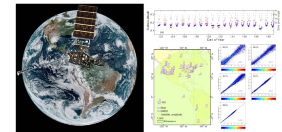
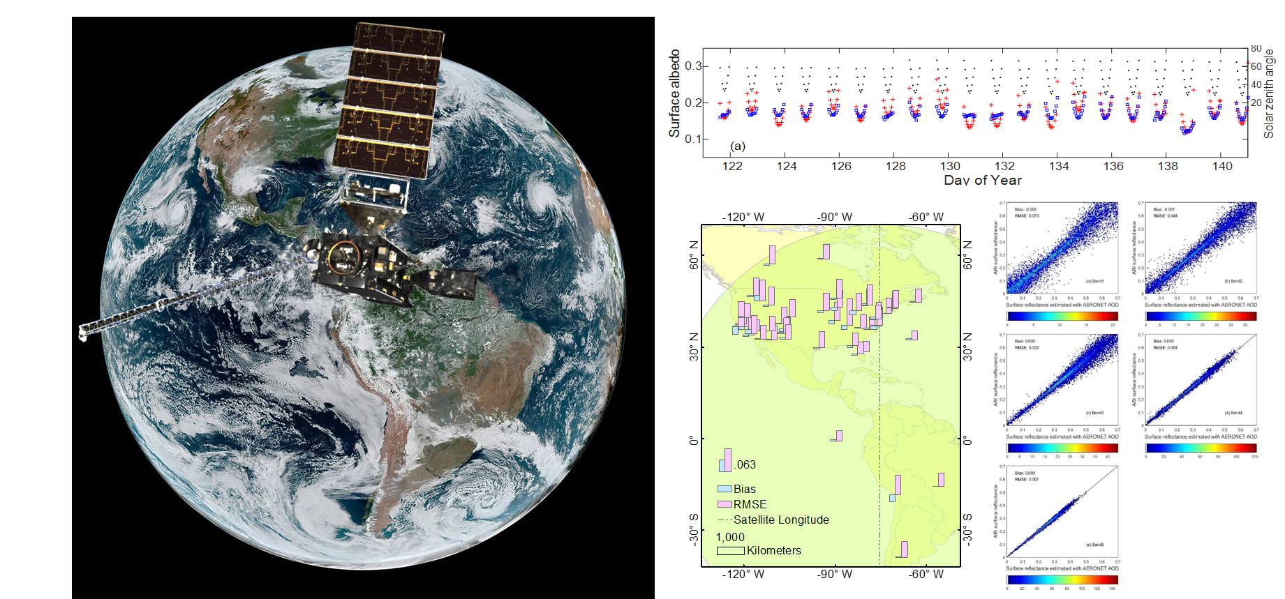
2.2.1. GOES-R ABI and Himawari AHI Data

GOES-16 is the first satellite in the GOES-R series, launched in November 2016 and operated by NOAA, entered operational service on 18 December 2017. Its operational location is 75.2°W, and it covers the majority of North, Central and South America. The ABI sensor onboard GOES-16 has six bands in the shortwave range (0.47 µm, 0.64 µm, 0.86 µm, 1.37 µm, 1.6 µm, 2.2 µm) with nadir spatial resolutions of 0.5 km, 1 km, and 2 km. All the bands, except for the 1.37 µm band designed for cirrus cloud detection, are included in the surface albedo retrieval processes in this study.

Himawari-8 is a Japanese geostationary satellite operated by the Japan Meteorological Agency, which was launched on 7 October 2014 and entered operational service on 7 July 2015. It carries the AHI sensor, with six bands in the shortwave range (0.47 µm, 0.51 µm, 0.64 µm, 0.86 µm, 1.6 µm, and 2.3 µm) at nadir spatial resolutions of 0.5 km, 1 km, and 2 km. All the bands are included in the surface albedo retrieval processes in this study.

One-kilometer resolution TOA reflectance data resampled from the original GOES-16 ABI and Himawari-8 AHI were obtained from NOAA together with the cloud mask baseline products for both ABI and AHI data [39]. Around one year’s data from ABI (October 2017–September 2018) and AHI (March 2016–February 2017) observations were processed for evaluation and validation purpose. As the cloud mask algorithm has difficulties identifying clouds in low-sun conditions [40], TOA observations from the early morning or late afternoon (solar zenith angle larger than 75°) were not used to retrieve surface albedo.

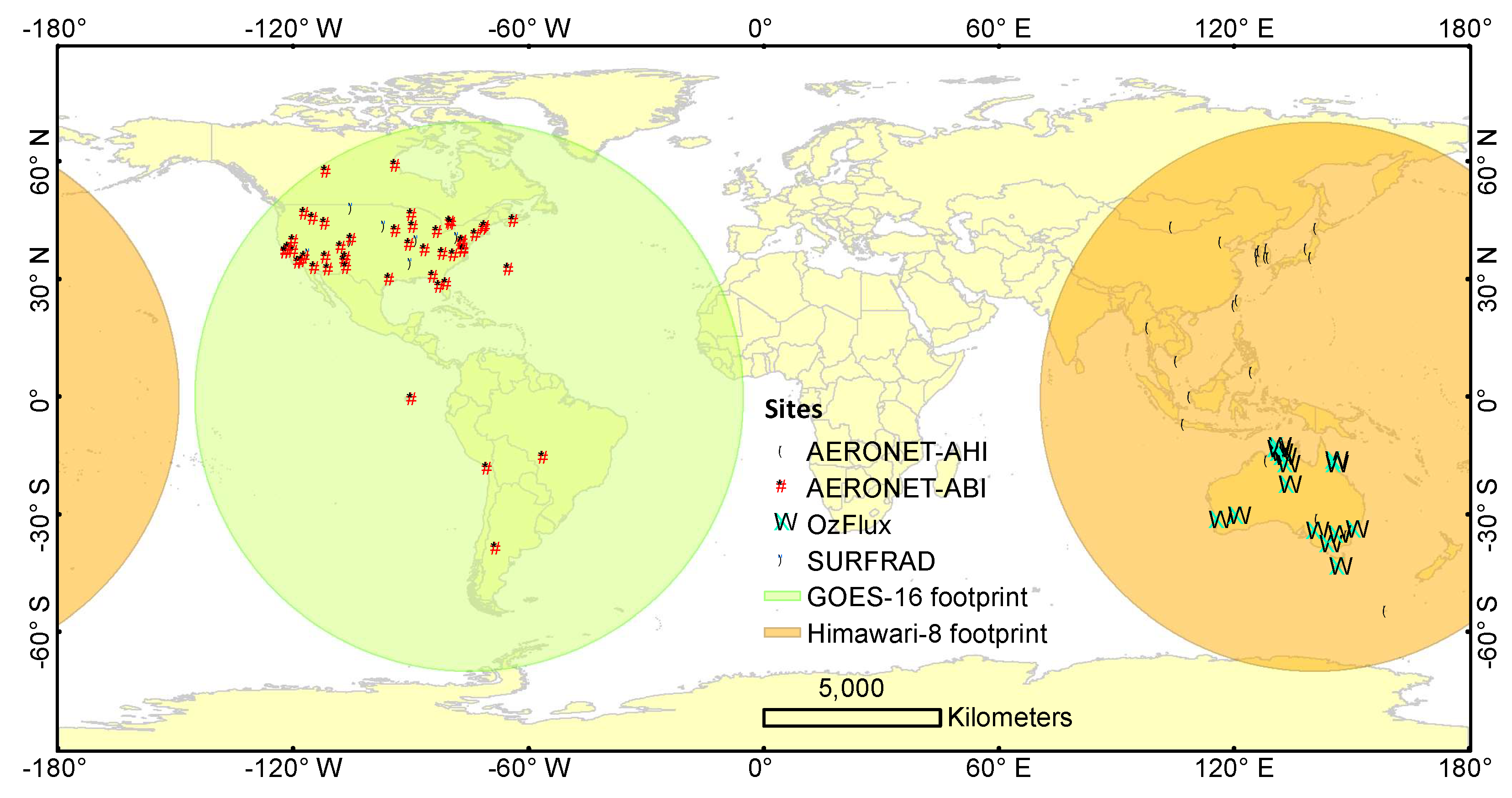
2.2.2. Ground Measurements

Ground measurements were used to validate the surface albedo and reflectance estimated from the geostationary satellites, including flux data from the Surface Radiation Budget Network (SURFRAD) sites and the OzFlux sites, as well as aerosol observations from the Aerosol Robotic Network (AERONET) sites (Figure 1).

SURFRAD is an observation network funded by NOAA. The SURFRAD mission is to support climate research with accurate, continuous, long-term measurements of the surface radiation budget over the United States. The albedo value is not directly measured at SURFRAD sites; ground measurements of downward and upward shortwave radiation from seven SURFRAD sites were used in this study to validate ABI albedo estimation. The recording cycle of SURFRAD is one minute.

The OzFlux network is a national network for the ecosystem, water, and energy balance researches located in Australia and New Zealand [41]. Ground measurements of downward and upward shortwave radiation are used for calculating surface albedo to validate the AHI-based albedo retrievals in this study. Thirteen sites are included in this research based on the data availability and quality.

Since field measurements for surface reflectance are scarcely available, we performed atmospheric correction with field observed aerosol optical depth (AOD) to obtain the reference values of surface reflectance. The AERONET [42] sites provide field observation for aerosol optical depth. We collected AOD data from 74 AERONET sites (50 within the ABI coverage and 24 within the AHI coverage) for validation. The reference values of surface reflectance were estimated from ABI and AHI clear-sky TOA observations and AERONET AOD observations through an independent atmospheric correction with the Ross–Li anisotropy kernel models from MODIS products [29,43].

2.2.3. Other Satellite Albedo Products

Three well-validated satellite albedo products were included in this study for accuracy intercomparison analysis, including MODIS, Visible Infrared Imaging Radiometer Suite (VIIRS), and Global Land Satellite System (GLASS) albedo products. The MODIS Collection 6 daily local noon surface albedo at local noon (MCD43A3) at 500 m spatial resolution obtained from https://earthdata.nasa.gov/ were resampled to 1km resolution for intercomparison [44]. The NOAA VIIRS daily surface albedo environment data record (EDR) products at 1 km spatial resolution [45] were obtained from https://www.avl.class.noaa.gov/saa/products/welcome. The GLASS version 4 albedo products [46] provide long term spatial and temporal continuous 8-day surface local noon albedo estimates at 1km spatial resolution were also included for intercomparison, which are available from http://www.glass.umd.edu/.

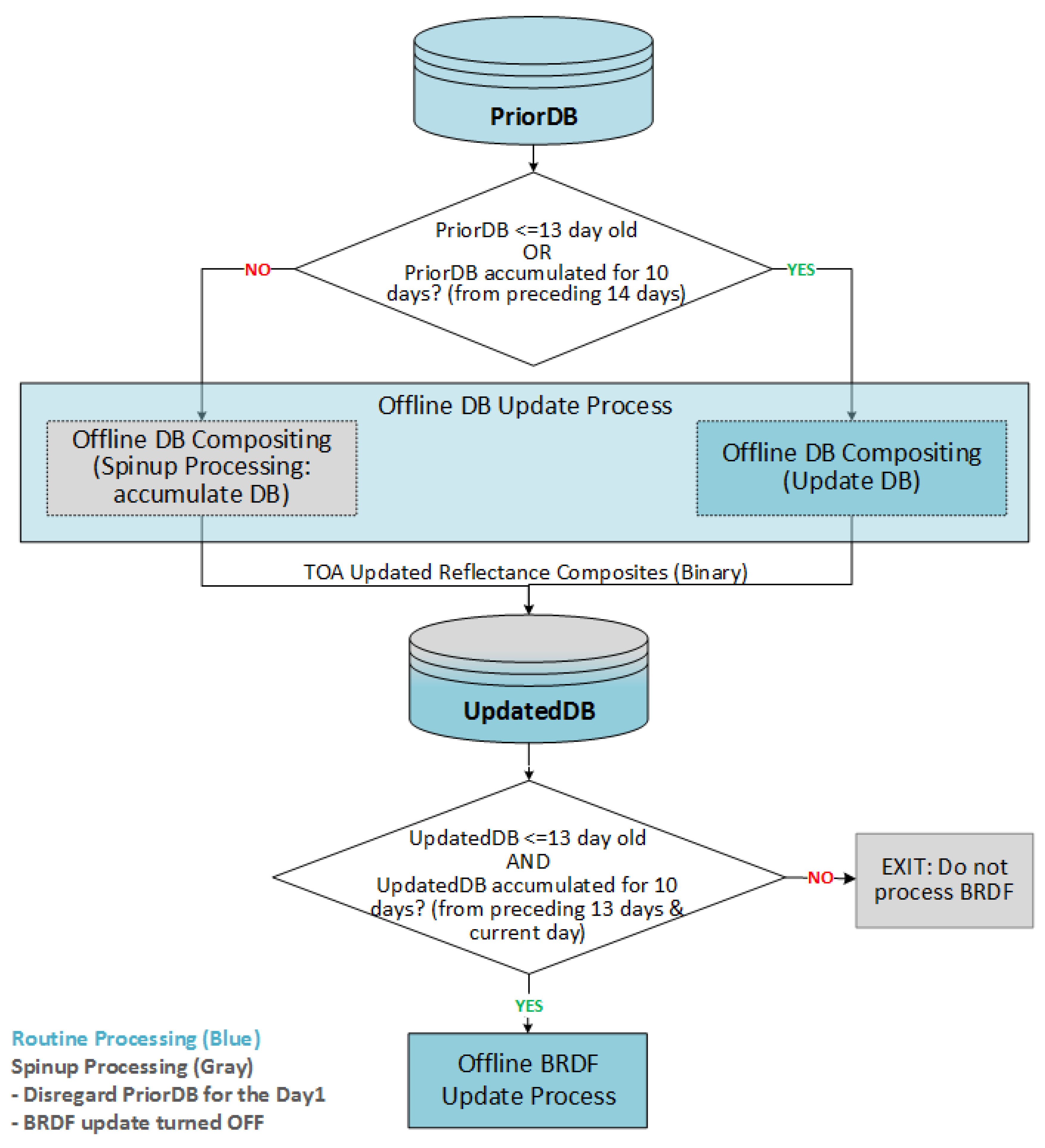
2.3. Operational Algorithm Implementation

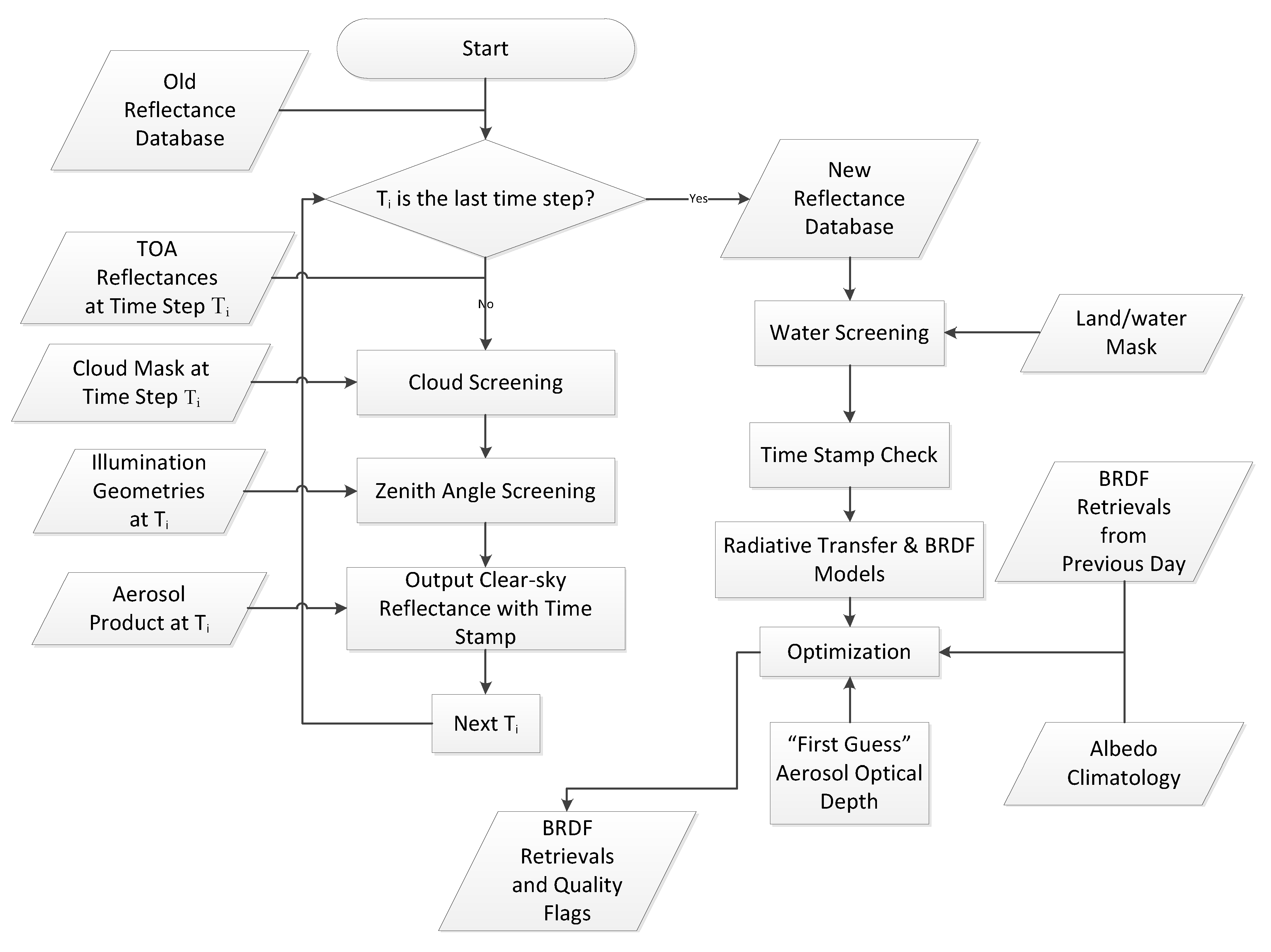
2.3.1. GOES-R Surface Albedo Product Suite Routine Processing Outline

Based on the theoretical basis, the algorithm was integrated into the NOAA system to produce the GOES-R surface albedo product suite. The retrieval of BRDF parameters needs multiple observations with different viewing geometries. Since ABI is not a multi-angular sensor, we achieve this by using a stack of time series observations over each pixel within a short period of time to create a reflectance database. Such a BRDF database consists of diurnal hourly clear-sky TOA reflectance values (24 values), which is updated daily, and the BRDF retrieval process is repeated once every day with the up-to-date BRDF database. To reduce the effect of rapid surface changes, TOA reflectance beyond 14 days is not considered in the retrieval process.

The organization of time series data and retrieval of BRDF parameters are time-consuming processes. To improve efficiency, we divide our algorithm into two parts: the offline mode and the online mode. At the end of each day, an offline mode computation is conducted to perform a full inversion of BRDF parameters using the stacked time series data at 1-h intervals. The surface albedo algorithm will take the GOES-R AOD product as the “first-guess” values. Our strategy is to estimate the land surface BRDF parameters and update AOD information simultaneously based on the initial estimates of AOD and albedo climatology. The calculated BRDF parameters are saved for the usage of the online mode the next day ideally. The processing chains of the GOES-R surface albedo offline algorithm are shown in Figure 2.

The pre-calculated BRDF parameters are used to derive full disk surface albedo products every 60 min in the online mode. In addition to albedo, surface reflectance will also be generated every 60 min in the online mode using the retrieved BRDF model parameters from the offline mode. Although ABI and AHI have refreshing rates finer of 15 min, the surface albedo and reflectance products are required to be generated every 60 min in the NOAA system. For the sake of operational latency requirement, the online mode will select observations closest to each exact hour to calculate albedo and reflectance.

2.3.2. Startup Setup and Interruption Control

Automatic control handling strategy needs to be designed in case of systematic exceptions. For instance, the offline algorithm relies on an accumulation of clear-sky TOA observations to composite the BRDF (Figure 3). The timeliness of the TOA reflectance will influence the BRDF accuracy, so it is necessary to consider how to deal with TOA data missing or system interruptions. Besides, the BRDF optimization algorithm needs reliable initial value input to improve efficiency and effectiveness. When the BRDF from the previous day is available, it can provide the initial value for the optimization. Otherwise, the algorithm will switch to an experienced initial value and broader searching range to achieve the globally optimized coefficients. The applied exception handling strategy is introduced in this section, which also guides the setup method for a startup status of the near-real time operation.

2.3.3. Data Availability-Oriented Branches

The online albedo/reflectance retrieval requires the offline produced BRDF as input. The BRDF retrieval relies on an accumulation of TOA reflectance within a composition period. Typically, one days’ observations have enough angular samplings to drive the BRDF retrievals. However, due to the cloud contamination and the geometry angle restriction, many pixels still lack enough reflectance observations after one day. Then, the latest available clear-sky TOA reflectance works as a substitute. However, the time gap cannot be longer than 14 days so that the assumption of BRDF stability remains valid. Thus, each set-up process starts with an accumulation of database for ten days to make sure the clear-sky TOA reflectance dataset is available for most pixels. Before the completion of this spin-up period, the BRDF retrieval sub-module will not be executed (Figure 3).

2.3.4. Seed Data Handling Strategy

The offline algorithm deploys an optimization process to estimate the BRDF parameters. The BRDF coefficients from the previous day act as an initial value in the optimization process accompanying a surrounding searching range in the response surface of the objective function. The previous BRDF is adopted as prior knowledge in the optimization which will help accelerate the convergence. Otherwise, if the previous BRDF coefficients are not available, the algorithm uses an experienced initial value and a wider searching range in the response surface. According to our test, both situations will reach the global optimum with available input datasets. However, the latter has a longer running time. The initial values and searching range of BRDF coefficients are listed in

Table 3. Initial values and searching ranges of BRDF kernel parameters in the retrieval process.

	Fiso		Fvol		Fgeo
	Initial	Range	Initial	Range	Initial	Range
with previous BRDF	fiso-pre	[initial − 0.2, initial + 0.2]	fvol-pre	[initial − 0.1, initial + 0.1]	fgeo-pre	[initial − 0.05, initial + 0.05]
without previous BRDF	0.2	[0,1]	0.1	[0,0.4]	0.05	[0,0.1]

.

3. Results and Discussion

The GOES-R albedo/reflectance product suite algorithm was evaluated with ABI data and also tested with AHI data. We validated the albedo product with one year of ABI and AHI data against field measurements and existing satellite albedo products including MODIS, VIIRS, and GLASS products. We also performed atmospheric correction at more than 80 AERONET sites with field observed AOD to obtain reflectance as reference values, and then compared the reflectance product against the atmospherically corrected reflectance. One year of ABI (October 2017–September 2018) and AHI (March 2016–February 2017) data were processed for the validation and product intercomparison.

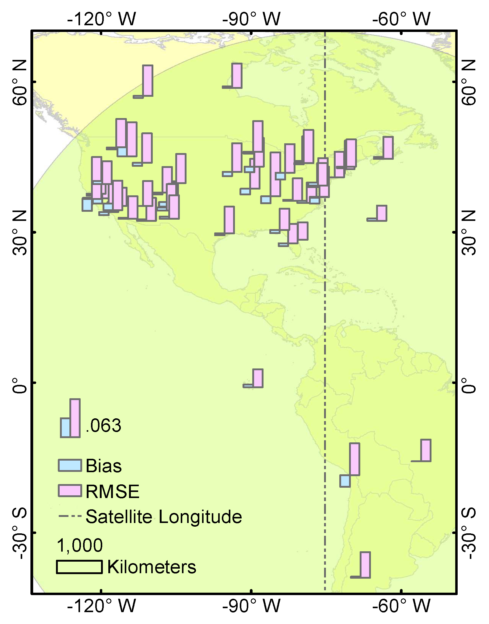
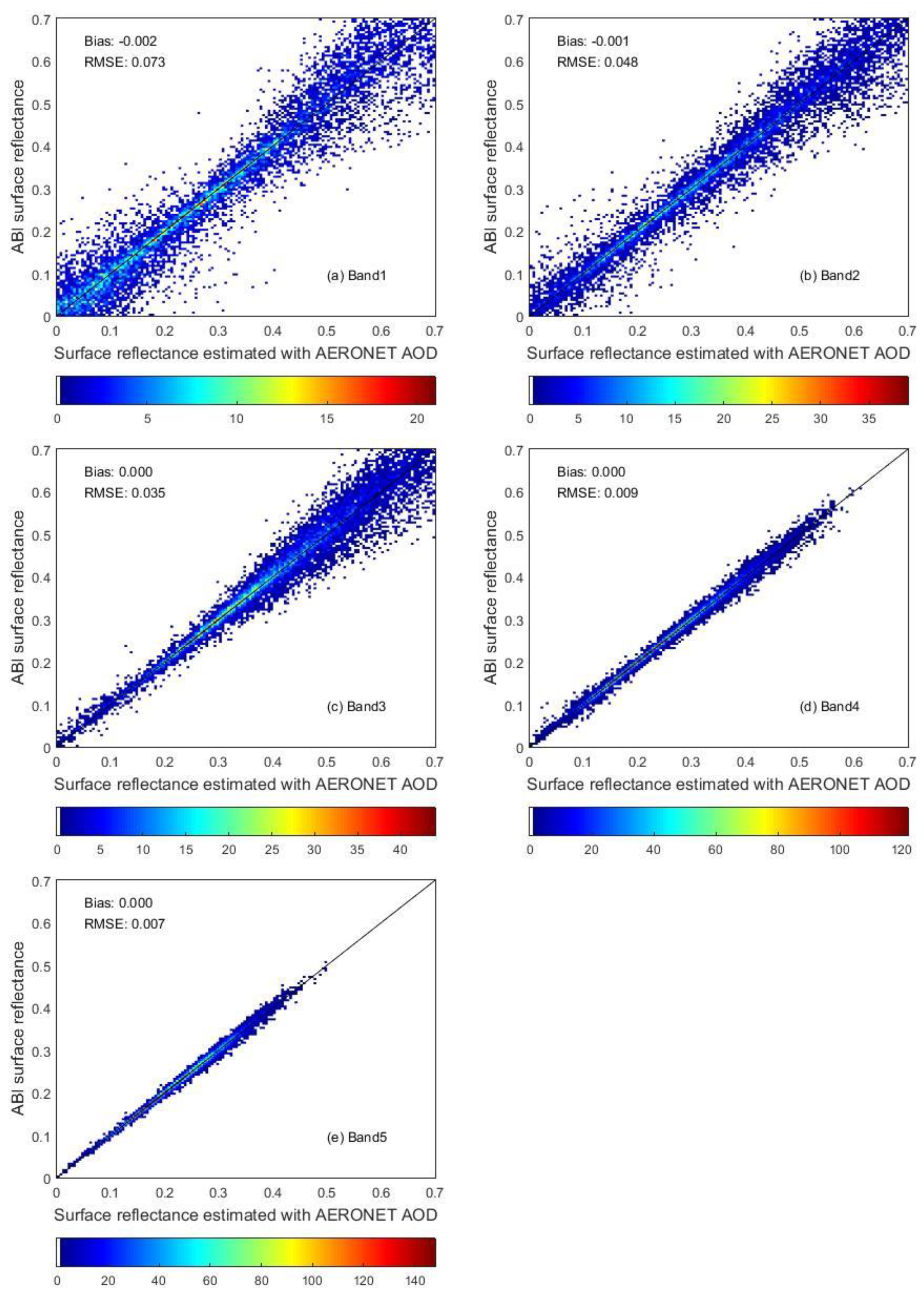
3.1. ABI-Based Albedo Validation and Intercomparison

We performed two analyses in evaluating the ABI-based albedo estimation. We first validated the hourly ABI albedo against SURFRAD site measurements and then compared the accuracy of MODIS, VIIRS, GLASS, and ABI albedo products at the daily temporal resolution.

Table 4. Hourly ABI albedo validation results at SURFRAD sites.

Site	Bias	RMSE
Fort Peck	0.005	0.049
Sioux Falls	−0.005	0.046
Penn State	−0.009	0.053
Bondville	−0.008	0.072
Boulder	0.011	0.054
Desert Rock	0.012	0.033
Goodwin Creek	−0.007	0.032
All (N = 18104)	−0.000	0.050

shows the validation statistics of hourly clear-sky surface albedo against ground measurements. Generally, the ABI surface albedo estimation had a very small bias with an RMSE of 0.050 and a relative RMSE (RMSE of the relative difference between satellite retrievals and ground measurements) of 19.8%. Five sites have absolute bias values lower than 0.010. The largest RMSE was found at the Bondville site, which is an agriculture site in Illinois, US, with spatial heterogeneity issues from the ephemeral snow events and the wet drainage system around the site [47].

An example of diurnal clear-sky albedo time series during early May 2017 from ABI data and ground measurements at SURFRAD sites is provided because of the good clear-sky data availability and is shown in Figure 4. Both the diurnal and intraday albedo variations in surface albedo were reasonably captured by the ABI retrievals, while the temporal diurnal variation in satellite estimation is slightly larger in the early morning and late afternoon. Spatial heterogeneity issues can be identified at the sites of Sioux Falls, Bondville, and Goodwin Creek, which has been reported in [47] using Landsat data. Data gaps at Boulder site (Figure 4e) were caused by continuous cloud coverage during the time period.

In the validation of local noon albedos (

Table 5. Local noon albedo validation results at SURFRAD sites.

Site	ABI		MODIS		VIIRS		GLASS
	Bias	RMSE	Bias	RMSE	Bias	RMSE	Bias	RMSE
Fort Peck	0.004	0.040	−0.031	0.059	−0.035	0.078	−0.045	0.097
Sioux Falls	−0.004	0.032	0.015	0.080	0.021	0.074	0.027	0.108
Penn State	−0.012	0.036	−0.089	0.111	−0.042	0.062	−0.066	0.085
Bondville	−0.018	0.045	−0.058	0.085	−0.060	0.090	−0.080	0.117
Boulder	0.008	0.035	−0.009	0.031	−0.012	0.040	−0.039	0.105
Desert Rock	−0.003	0.017	−0.027	0.028	0.016	0.031	−0.004	0.020
Goodwin Creek	−0.009	0.027	−0.055	0.059	−0.035	0.046	−0.049	0.054
All (N = 985)	−0.004	0.032	−0.033	0.064	−0.016	0.060	−0.032	0.085

), the ABI albedo provides an overall RMSE of 0.032, followed by VIIRS albedo (0.060), MODIS (0.064), and GLASS albedo (0.085). The results are not surprising because the geostationary satellite can have multiple clear-sky observations during a short period and thus it has an improved ability to capture the surface changes compared with albedo estimation from polar-orbiting satellites. Analysis was conducted on the four albedo products over two sites of Fort Peck and Desert Rock with less surface heterogeneity compared to the other sites [47]. Large RMSE values for MODIS, VIIRS, and GLASS albedos were mostly from undetected snow cases, because these albedo products used information from either an 8-day or a 16-day window for temporal smoothing or compositing. Such information from a long temporal period will affect the detection of some ephemeral snow cases.

Figure 5 and

Table 6. ABI reflectance validation results at AERONET sites.

Site	Bias	RMSE	Site	Bias	RMSE
Marina	−0.011	0.059	Rexburg_Idaho	−0.005	0.048
Ames	−0.007	0.047	Rimrock	0.003	0.050
Appalachian_State	0.002	0.037	SP_Bayboro	−0.004	0.032
Arica	−0.019	0.052	San_Cristobal_USFQ	0.004	0.029
Billerica	−0.006	0.047	Sandia_NM_PSEL	0.008	0.038
CEILAP-Neuquen	0.002	0.042	Santa_Monica_Colg	−0.005	0.048
CUIABA-MIRANDA	0.000	0.036	Sevilleta	0.005	0.043
Churchill	0.003	0.040	St_Louis_University	−0.009	0.049
Denver_LaCasa	0.003	0.048	TABLE_MOUNTAIN_CA	0.011	0.048
EPA-Res_Triangle_Pk	0.003	0.033	Tallahassee	−0.005	0.035
Egbert	−0.003	0.040	Taylor_Ranch_TWRS	0.015	0.056
Fort_McKay	−0.003	0.050	TWRS	0.015	0.056
Fresno_2	−0.009	0.052	Thompson_Farm	−0.003	0.044
GSFC	0.000	0.039	Toronto	−0.002	0.054
Goldstone	0.006	0.030	Tucson	0.003	0.038
Halifax	0.003	0.036	Tudor_Hill	0.004	0.025
Hampton_University	−0.011	0.050	UMBC	0.005	0.037
IMPROVE-MammothCave	−0.011	0.072	USGS_Flagstaff_ROLO	0.000	0.041
LISCO	0.000	0.042	U_of_Wisconsin_SSEC	−0.009	0.047
Lake_Erie	−0.011	0.047	Wisconsin	−0.003	0.050
MD_Science_Center	0.003	0.045	Univ_of_Houston	−0.003	0.044
Modesto	−0.003	0.048	Univ_of_Nevada-Reno	0.005	0.038
Monterey	−0.019	0.069	White_Sands_HELSTF	0.004	0.039
NASA_KSC	0.000	0.029	Yuma	0.002	0.037
NASA_LaRC	−0.002	0.041
Red_Mountain_Pass	−0.003	0.042	All sites (N = 55755)	0.000	0.042

show the reflectance validation results against AERONET AOD corrected surface reflectance values. The ABI surface reflectance agrees well with atmospherically corrected surface reflectance. The overall RMSE is 0.042 with a bias very close to zero. The site-level bias and RMSE ranges from −0.019 to 0.015 and from 0.025 to 0.072, respectively. Most of the sites have absolute bias and RMSE below 0.010 and 0.050, respectively. There does not seem to be any obvious spatial pattern of bias and RMSE in Figure 5. The directional reflectance estimation does not seem to have any significant band dependence of bias with an overall RMSE value of 0.042 (13.6% in terms of relative RMSE) (Figure 6). However, band 1 (0.47 µm) and band 2 (0.64 µm) have larger RMSE because of the higher atmospheric effects, which were not fully corrected in our estimation process. In addition, ephemeral snow events can affect the reflectance estimation as larger differences can be found for the higher values in the visible and near-infrared bands. During winter seasons, many pixels were covered by clouds and snow, making it difficult to accumulate reliable clear-sky observations in the retrieval process. In such cases, it is likely that some of the BRDF retrievals were estimated based on observations from multiple days before the “current” day, while the reference surface reflectance data were estimated with satellite observation and AERONET AOD from the “current” day, leading to large differences in surface reflectance shown in Figure 6.

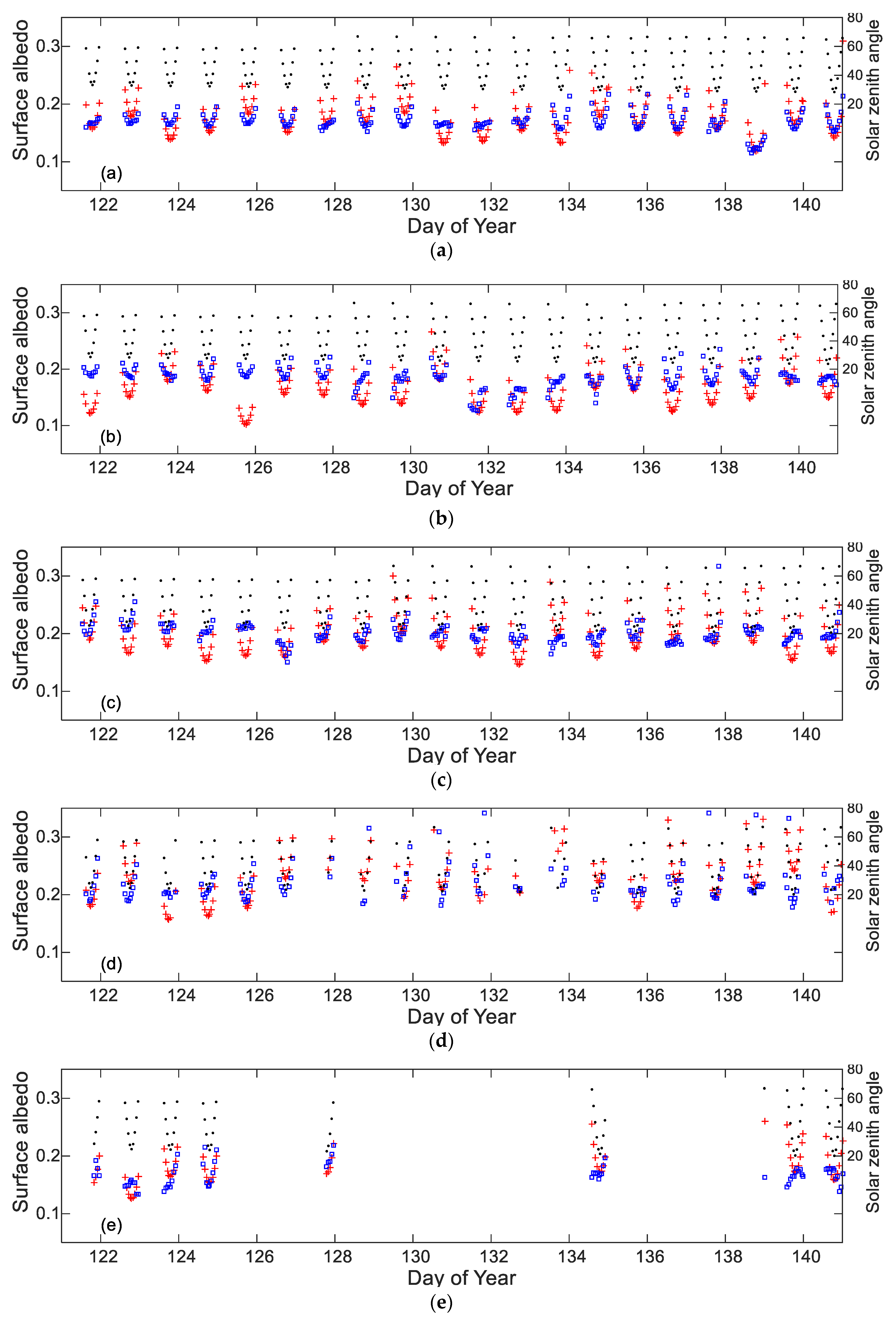
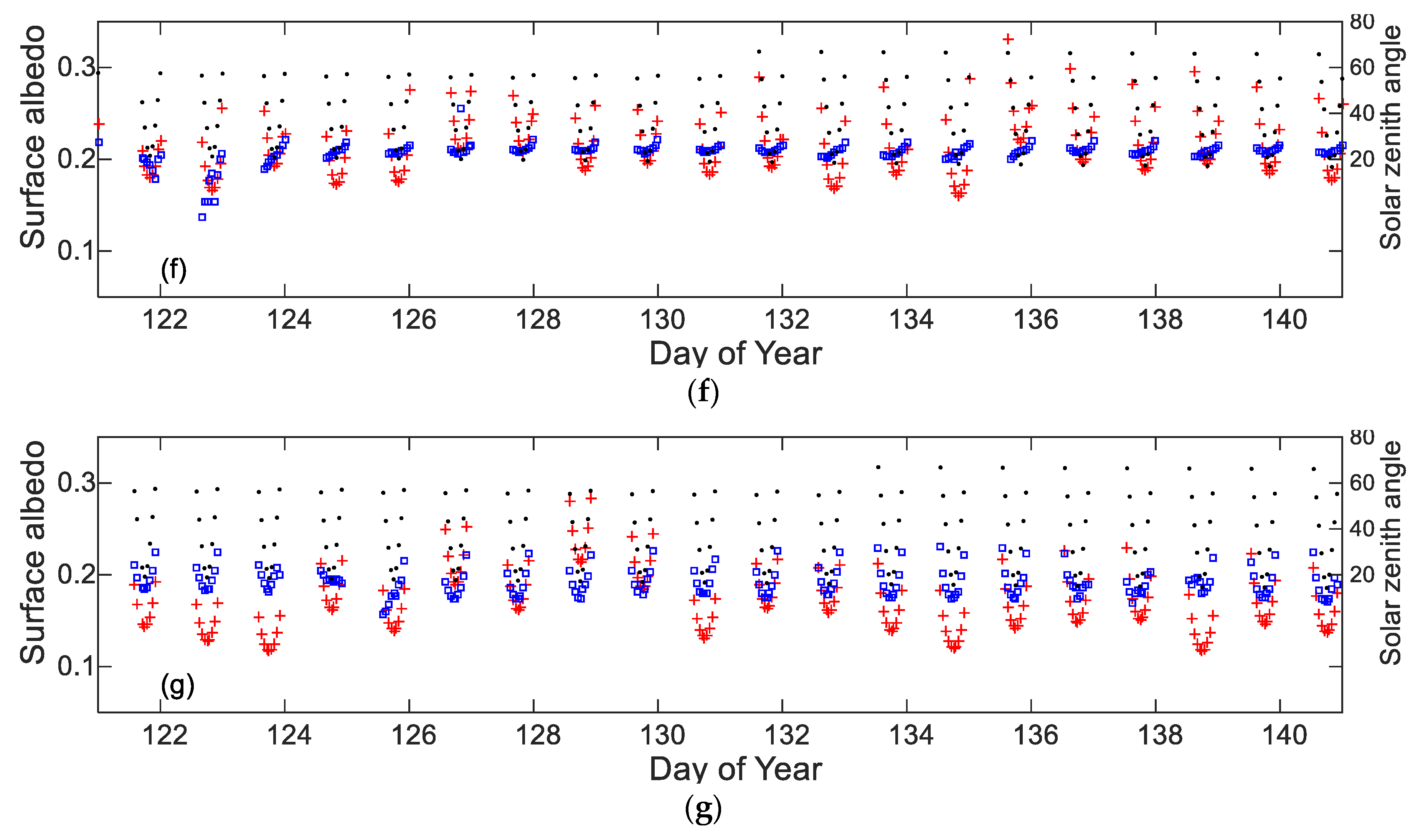
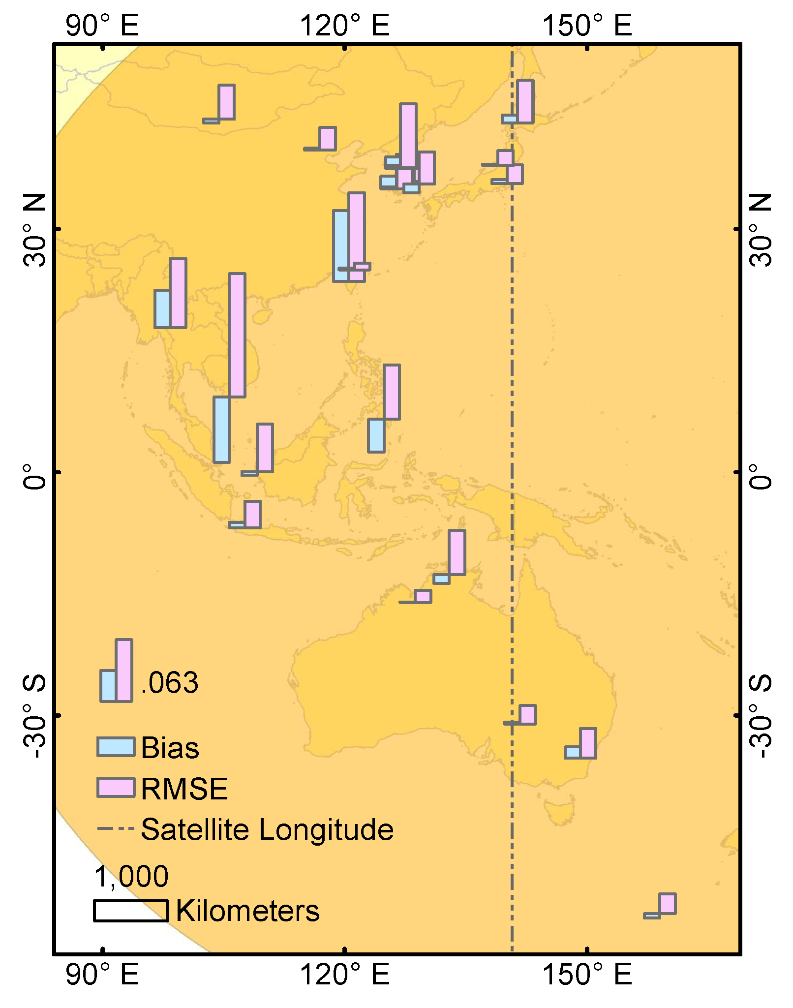
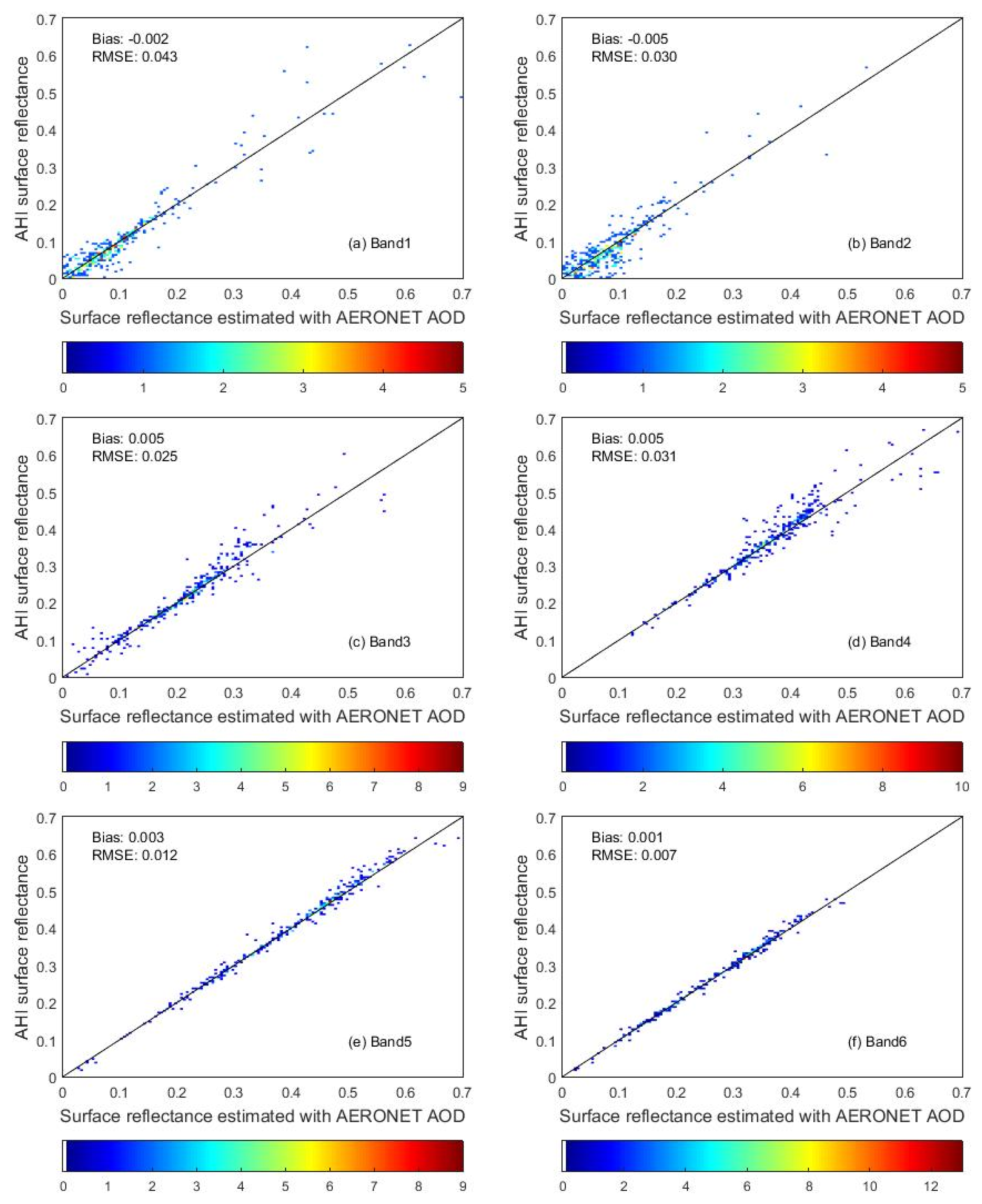
3.2. AHI-Based Albedo and Reflectance Validation and Intercomparison

Similar to the ABI results, we performed two analyses in evaluating the AHI-based albedo estimation. We first validated the hourly AHI albedo against OzFlux site measurements and then compared the accuracy of MODIS, VIIRS, GLASS, and AHI albedo products at the daily temporal resolution.

Table 7. Hourly AHI albedo validation results against OzFlux sites.

Site	Bias	RMSE
Calperum	−0.027	0.045
CowBay	−0.053	0.072
CumberlandPlain	0.081	0.090
DalyUncleared	0.044	0.060
Gingin	0.019	0.043
GWW	0.018	0.049
HowardSprings	0.035	0.052
Robson	0.051	0.066
SturtPlains	−0.040	0.073
Tumbarumba	0.052	0.063
Warra	0.085	0.093
WombatStateForest	0.013	0.048
Yanco	−0.034	0.054
All sites (N = 29546)	0.020	0.065

and

Table 8. Local noon albedo validation results at OzFlux sites.

Site	AHI		MODIS		VIIRS		GLASS
	Bias	RMSE	Bias	RMSE	Bias	RMSE	Bias	RMSE
Calperum	−0.042	0.051	−0.036	0.039	−0.021	0.060	−0.043	0.046
CowBay	−0.057	0.068	−0.087	0.089	−0.075	0.087	−0.090	0.091
CumberlandPlain	0.062	0.068	0.033	0.034	0.032	0.057	0.037	0.038
DalyUncleared	0.024	0.038	0.011	0.014	−0.010	0.028	0.010	0.014
Gingin	0.002	0.034	−0.029	0.031	−0.028	0.048	−0.016	0.019
GWW	0.002	0.040	−0.003	0.009	0.001	0.042	−0.018	0.020
HowardSprings	0.017	0.038	0.001	0.010	−0.013	0.031	−0.003	0.008
Robson	0.036	0.049	−0.007	0.009	0.004	0.028	0.010	0.011
SturtPlains	−0.042	0.052	−0.019	0.022	−0.074	0.081	−0.089	0.091
Tumbarumba	0.045	0.053	−0.014	0.018	0.002	0.026	0.020	0.021
Warra	0.072	0.078	0.010	0.017	0.054	0.133	−0.005	0.009
WombatStateForest	−0.005	0.051	0.004	0.008	0.017	0.078	0.015	0.016
Yanco	−0.037	0.053	−0.035	0.043	−0.023	0.058	−0.027	0.032
All sites (N = 1202)	0.008	0.050	−0.009	0.030	−0.011	0.056	−0.013	0.039

show the validation and intercomparison results.

AHI hourly albedo estimation was found to have a bias of 0.020 and an RMSE of 0.065, which is worse in statistics compared to the ABI site validation. At some sites, the large bias can be observed in Table 7, such as that for CowBay, CumberlandPlain, SturtPlain, and Warra, which led to large RMSEs reported here. This issue is also observed in the validation of the daily albedo estimation in Table 8. In general, our AHI-based local noon albedo has a bias of 0.008 and an RMSE of 0.050, which is comparable to VIIRS albedo products (RMSE: 0.056), and a little worse than the GLASS albedo products (RMSE: 0.041) and MODIS albedo products (RMSE: 0.30). The smaller differences among albedo products compared with the ABI-based albedo validation at SURFRAD sites are likely a result of much fewer snow events in the semi-arid area of OzFlux sites in Australia.

It should be noticed that many of the field sites have poor homogeneity and spatial representativeness and are not recommended for mesoscale surface albedo validation [44,48]. Based on the previous research, almost all of the OzFlux sites are not spatially homogeneous at the kilometer scale. Additional ground measurements at homogeneous sites are required to make solid validation results for the AHI-based albedo estimation.

Figure 7 and

Table 9. AHI reflectance validation results at AERONET sites.

Site	Bias	RMSE	Site	Bias	RMSE
ARM_Macquarie_Is	−0.013	0.022	KORUS_Kyungpook_NU	0.003	0.020
Canberra	0.011	0.030	KORUS_Mokpo_NU	0.002	0.027
Anmyon	−0.004	0.020	KORUS_UNIST_Ulsan	−0.009	0.032
Bac_Lieu	−0.066	0.125	Lake_Argyle	0.001	0.013
Bandung	0.006	0.027	ND_Marbel_Univ	−0.033	0.055
Chiayi	0.072	0.090	Niigata	0.001	0.015
Chiba_University	0.004	0.019	Omkoi	0.038	0.070
Dalanzadgad	−0.004	0.034	Pontianak	−0.004	0.048
EPA-NCU	0.002	0.007	Seoul_SNU	0.012	0.029
Fowlers_Gap	0.002	0.019	XiangHe	0.002	0.023
Gangneung_WNU	−0.004	0.005	Yonsei_University	0.002	0.065
Hokkaido_University	0.008	0.043
Jabiru	−0.009	0.045	All sites (N = 2160)	0.001	0.027

show the reflectance validation results at AERONET sites. The AHI surface reflectance agrees well with atmospherically corrected surface reflectance using AERONET AOD values. The overall RMSE is 0.027 (19.9% in terms of relative RMSE), lower than that of ABI surface reflectance. Large bias and RMSE values are found at sites located around cities in East Asia, possibly due to under/overcorrection of large aerosol loading in those areas (Figure 7). Similar to the ABI results, RMSE values are larger for the visible bands (band 1: 0.47 µm, band 2: 0.51 µm, and band 3: 0.64 µm) than for the infrared bands (Figure 8). Meanwhile, the RMSE values for the visible bands of AHI are lower than those for the ABI bands, possibly a result of the additional spectral information provided by the green band (0.51 µm) in AHI data; however, it should be noted that the sample size for the AHI validation is much smaller than that for the ABI validation.

4. Conclusions

Geostationary satellites provide a unique means to observe the Earth’s surface at very high temporal resolutions, and can thus better capture the changes in surface albedo within a short period than polar orbiting satellites. The approach proposed in this study as a prototype for the NOAA GOES-R ABI surface directional reflectance and albedo product suite algorithm, used GOES-16 ABI and Himawari-8 AHI data to evaluate its performance. With the very high temporal resolution of geostationary observations, it is much easier to obtain sufficient cloud free angular samples over the same location within a short period of time. The original algorithm proposed for MODIS data needs multiple days to accumulate enough clear sky information, while in this study, the refined algorithm used the daily-updated observations to reflect the most recent state of surface anisotropy.

Unlike polar-orbiting satellites, which usually observe the same location under similar solar zenith angles but different viewing angles within the temporal composite window (because of the same overpass time), geostationary platforms provide information with fixed viewing geometries, while the solar illumination direction changes. One of the basic assumptions in estimating surface albedo from geostationary data is that the surface anisotropy follows the reciprocity principle, so that the BRF kernel models can be used and the surface albedo estimations can be compared with to the MODIS and other polar-orbiting satellite products. Generally, this study showed reasonable results when comparing the retrieved albedo from this approach with ground measurements and other existing satellite products, including MODIS, VIIRS, and GLASS data. However, it has to be pointed that using the ground measurements of radiative fluxes is not an ideal way to assess kilometer scale surface albedo estimation from satellite data for most of the sites due to their footprint differences. More work is still needed to bridge the gap between coarse resolution data and ground measurements, possibly with the help of medium to fine resolution albedo data [49].

Compared to the original algorithm applied to MODIS data, a very important improvement obtained by using ABI and AHI data rather than MODIS data is that the ABI and AHI observations can provide information on the diurnal changes in surface albedo. This study shows that the proposed algorithm has good accuracy overall in capturing the diurnal changes in albedo that are caused mainly by the solar illumination angle and aerosol loadings. Moreover, the diurnal albedo information can be used to estimate the energy budget in the shortwave range on a daily basis, while it would be difficult to do with data from polar-orbiting satellites due to their reduced temporal resolution and lack of observations for early morning and late afternoon. Instantaneous albedo estimations have larger uncertainties with increased solar zenith angles, either due to the failure of surface BRF models or potential residual cloud contaminations.

In this study, we have shown that the albedo and reflectance estimation with GOES-R data can achieve the accuracy requirement for downstream meteorological and climate applications. For example, the World Meteorology Organization (WMO) lists the threshold accuracy requirement of surface albedo for high-resolution national weather service as 20% (https://www.wmo-sat.info/oscar-staging/requirements). There is still a need to further improve the product to achieve the 10% breakthrough accuracy proposed by WMO. More efforts are needed, including extensive validation activities with higher resolution remotely sensed data as a bridge over heterogeneous areas, as well as further algorithm improvement during periods when rapid surface changes take place.

References

1. Liang, S.; Wang, D.; He, T.; Yu, Y. Remote sensing of Earth’s energy budget: Synthesis and review. Int. J. Digit. Earth 2019, 737–780. [Google Scholar] [CrossRef]
2. Lattanzio, A.; Schulz, J.; Matthews, J.; Okuyama, A.; Theodore, B.; Bates, J.J.; Knapp, K.R.; Kosaka, Y.; Schüller, L. Land surface albedo from geostationary satellites: A multiagency collaboration within SCOPE-CM). Bull. Am. Meteorol. Soc. 2013, 94, 205–214. [Google Scholar] [CrossRef]
3. de Wildt, M.D.; Gabriela, S.; Gruen, A. Operational snow mapping using multitemporal Meteosat SEVIRI imagery. Remote Sens. Environ. 2007, 109, 29–41. [Google Scholar] [CrossRef]
4. Proud, S.R.; Fensholt, R.; Rasmussen, R.V.; Sandholt, I. Rapid response flood detection using the MSG geostationary satellite. Int. J. Appl. Earth Obs. Geoinf. 2011, 13, 536–544. [Google Scholar] [CrossRef]
5. Romanov, P.; Tarpley, D.; Gutman, G.; Carroll, T. Mapping and monitoring of the snow cover fraction over North America. J. Geophys. Res. Atmos. 2003, 108. [Google Scholar] [CrossRef]
6. Yan, X.; Li, Z.; Luo, N.; Shi, W.; Zhao, W.; Yang, X.; Jin, J. A minimum albedo aerosol retrieval method for the new-generation geostationary meteorological satellite Himawari-8. Atmos. Res. 2018, 207, 14–27. [Google Scholar] [CrossRef]
7. Trigo, I.F.; Bruin, H.; Beyrich, F.; Bosveld, F.C.; Gavilán, P.; Groh, J.; López-Urrea, R. Validation of reference evapotranspiration from Meteosat Second Generation (MSG) observations. Agric. For. Meteorol. 2018, 259, 271–285. [Google Scholar] [CrossRef]
8. Damiani, A.; Irie, H.; Horio1, T.; Takamura, T.; Khatri, P.; Takenaka, H.; Nagao, T.; Nakajima, T.Y.; Cordero, R.R. Evaluation of Himawari-8 surface downwelling solar radiation by ground-based measurement. Atmos. Meas. Tech. 2018, 11, 2501–2521. [Google Scholar] [CrossRef]
9. Zou, X.; Zhuge, X.; Weng, F. Characterization of bias of Advanced Himawari Imager infrared observations from NWP background simulations using CRTM and RTTOV. J. Atmos. Ocean. Technol. 2016, 33, 2553–2567. [Google Scholar] [CrossRef]
10. Csiszar, I.; Gutman, G. Mapping global land surface albedo from NOAA AVHRR. J. Geophys. Res. Atmos. 1999, 104, 6215–6228. [Google Scholar] [CrossRef]
11. Diner, D.J.; Martonchik, J.V.; Borel, C.; Gerstl, S.A.W.; Gordon, H.R.; Knyazikhin, Y.; Myneni, R.; Pinty, B.; Verstraete, M.M. Level 2 Surface Retrieval Algorithm Theoretical Basis Document. In NASA/JPL JPL D-11401 Rev. E; 2008. Available online: https://eospso.gsfc.nasa.gov/sites/default/files/atbd/ATB_L2Surface43.pdf (accessed on 20 September 2019).
12. Leroy, M.; Deuzé, J.L.; Bréon, F.M.; Hautecoeur, O.; Herman, M.; Buriez, J.C.; Tanré, D.; Bouffiès, S.; Chazette, P.; Roujean, J.L. Retrieval of atmospheric properties and surface bidirectional reflectances over land from POLDER/ADEOS. J. Geophys. Res. Atmos. 1997, 102, 17023–17037. [Google Scholar] [CrossRef]
13. Schaaf, C.B.; Gao, F.; Strahler, A.H.; Lucht, W.; Li, X.; Tsang, T.; Strugnell, N.C.; Zhang, X.; Jin, Y.; Muller, J.P. First operational BRDF, albedo nadir reflectance products from MODIS. Remote Sens. Environ. 2002, 83, 135–148. [Google Scholar] [CrossRef]
14. Wang, D.; Liang, S.; Zhou, Y.; He, T.; Yu, Y. A new method for retrieving daily land surface albedo from VIIRS data. IEEE Trans. Geosci. Remote Sens. 2017, 55, 1765–1775. [Google Scholar] [CrossRef]
15. He, T.; Liang, S.; Song, D.X. Analysis of global land surface albedo climatology and spatial-temporal variation during 1981-2010 from multiple satellite products. J. Geophys. Res. Atmos. 2014, 119, 10281–10298. [Google Scholar] [CrossRef]
16. Carrer, D.; Moparthy, S.; Lellouch, G.; Ceamanos, X.; Pinault, F.; Coelho, S.; Trigo, I. Land surface albedo derived on a ten daily basis from Meteosat Second Generation observations: The NRT and climate data record collections from the EUMETSAT LSA SAF. Remote Sens. 2018, 10, 1262. [Google Scholar] [CrossRef]
17. Geiger, B.; Carrer, D.; Franchisteguy, L.; Roujean, J.L.; Meurey, C. Land surface albedo derived on a daily basis from Meteosat Second Generation observations. IEEE Trans. Geosci. Remote Sens. 2008, 46, 3841–3856. [Google Scholar] [CrossRef]
18. Pinty, B.; Roveda, F.; Verstraete, M.M.; Gobron, N.; Govaerts, Y.; Martonchik, J.V.; Dine, D.J.; Kahn, R.A. Surface albedo retrieval from Meteosat—1. Theory. J. Geophys. Res. Atmos. 2000, 105, 18099–18112. [Google Scholar] [CrossRef]
19. Kaufman, Y.J.; Tanre, D.; Remer, L.A.; Vermote, E.F.; Chu, A.; Holben, B.N. Operational remote sensing of tropospheric aerosol over land from EOS moderate resolution imaging spectroradiometer. J. Geophys. Res. Atmos. 1997, 102, 17051–17067. [Google Scholar] [CrossRef]
20. Knapp, K.R.; Frouin, R.; Kondragunta, S.; Prados, A. Toward aerosol optical depth retrievals over land from GOES visible radiances: Determining surface reflectance. Int. J. Remote Sens. 2005, 26, 4097–4116. [Google Scholar] [CrossRef]
21. Popp, C.; Hauser, A.; Foppa, N.; Wunderle, S. Remote sensing of aerosol optical depth over central Europe from MSG-SEVIRI data and accuracy assessment with ground-based AERONET measurements. J. Geophys. Res. Atmos. 2007, 112. [Google Scholar] [CrossRef]
22. Govaerts, Y.; Wagner, S.; Lattanzio, A.; Watts, P. Joint retrieval of surface reflectance and aerosol optical depth from MSG/SEVIRI observations with an optimal estimation approach: 1. Theory. J. Geophys. Res. Atmos. 2010, 115. [Google Scholar] [CrossRef]
23. Smirnov, A.; Holben, B.N.; Eck, T.F.; Slutsker, I.; Chatenet, R.; Pinker, R.T. Diurnal variability of aerosol optical depth observed at AERONET (Aerosol Robotic Network) sites. Geophys. Res. Lett. 2002, 29. [Google Scholar] [CrossRef]
24. Wang, J.; Christopher, S.A.; Reid, J.S.; Maring, H.; Savoie, D.; Holben, B.N.; Livingston, J.M.; Russell, P.B.; Yang, S.K. GOES 8 retrieval of dust aerosol optical thickness over the Atlantic Ocean during PRIDE. J. Geophys. Res. Atmos. 2003, 108. [Google Scholar] [CrossRef]
25. Wang, J.; Xia, X.G.; Wang, P.C.; Christopher, S.A. Diurnal variability of dust aerosol optical thickness and Angstrom exponent over dust source regions in China. Geophys. Res. Lett. 2004, 31. [Google Scholar] [CrossRef]
26. Mei, L.; Xue, Y.; Leeuw, G.; Holzer-Popp, T.; Guang, J.; Li, Y.; Yang, L.; Xu, H.; Xu, X.; Li, C. Retrieval of aerosol optical depth over land based on a time series technique using MSG/SEVIRI data. Atmos. Chem. Phys. 2012, 12, 9167–9185. [Google Scholar] [CrossRef]
27. She, L.; Xue, Y.; Yang, X.; Leys, J.; Guang, J.; Che, Y.; Fan, C.; Xie, Y. Joint retrieval of aerosol optical depth and surface reflectance over land using geostationary satellite data. IEEE Trans. Geosci. Remote Sens. 2019, 57, 1489–1501. [Google Scholar] [CrossRef]
28. Zhang, Y.; He, T.; Liang, S.L.; Wang, D.D.; Yu, Y.Y. Estimation of all-sky instantaneous surface incident shortwave radiation from Moderate Resolution Imaging Spectroradiometer data using optimization method. Remote Sens. Environ. 2018, 209, 468–479. [Google Scholar] [CrossRef]
29. He, T.; Liang, S.L.; Wang, D.; Wu, H.; Yu, Y.; Wang, J. Estimation of surface albedo and directional reflectance from Moderate Resolution Imaging Spectroradiometer (MODIS) observations. Remote Sens. Environ. 2012, 119, 286–300. [Google Scholar] [CrossRef]
30. Liang, S.L.; Strahler, A.H. Retrieval of surface BRDF from multiangle remotely-sensed data. Remote Sens. Environ. 1994, 50, 18–30. [Google Scholar] [CrossRef]
31. Liang, S.L. Recent developments in estimating land surface biogeophysical variables from optical remote sensing. Prog. Phys. Geogr. 2007, 31, 501–516. [Google Scholar] [CrossRef]
32. Li, X.W.; Strahler, A.H. Geometric-optical bidirectional reflectance modeling of the DISCRETE crown vegetation canopy effect of crown shape and mutual shadowing. IEEE Trans. Geosci. Remote Sens. 1992, 30, 276–292. [Google Scholar] [CrossRef]
33. Roujean, J.L.; Leroy, M.; Deschamps, P.Y. A bidirectional reflectance model of the Earth’s surface for the correction of remote sensing data. J. Geophys. Res. Atmos. 1992, 97, 20455–20468. [Google Scholar] [CrossRef]
34. Qin, W.H.; Herman, J.R.; Ahmad, Z. A fast, accurate algorithm to account for non-Lambertian surface effects on TOA radiance. J. Gephys. Res. Atmos. 2001, 106, 22671–22684. [Google Scholar] [CrossRef]
35. Maignan, F.; Breon, F.M.; Lacaze, R. Bidirectional reflectance of Earth targets: Evaluation of analytical models using a large set of spaceborne measurements with emphasis on the Hot Spot. Remote Sens. Environ. 2004, 90, 210–220. [Google Scholar] [CrossRef]
36. Liang, S.L. Narrowband to broadband conversions of land surface albedo I Algorithms. Remote Sens. Environ. 2001, 76, 213–238. [Google Scholar] [CrossRef]
37. Clark, R.N.; Swayze, G.A.; Wise, R.A.; Eric Livo, K.; Hoefen, T.M.; Kokaly, R.F.; Sutley, S.J. USGS Digital Spectral Library Splib06a; U.S. Geological Survery, Digital Data Series: Reston, VA, USA, 2007.
38. Kotchenova, S.Y.; Vermote, E.F.; Matarrese, R.; Klemm, F.J. Validation of a vector version of the 6S radiative transfer code for atmospheric correction of satellite data. Part I: Path radiance. Appl. Opt. 2006, 45, 6762–6774. [Google Scholar] [CrossRef] [Green Version]
39. Heidinger, A.K.; Straka, W.C. Algorithm Theoretical Basis Document. In ABI Cloud Mask (Version 3.0); 2012. Available online: https://www.star.nesdis.noaa.gov/goesr/documents/ATBDs/Baseline/ATBD_GOES-R_Cloud_Mask_v3.0_July%202012.pdf (accessed on 20 September 2019).
40. Derrien, M.; Le Gleau, H. Improvement of cloud detection near sunrise and sunset by temporal-differencing and region-growing techniques with real-time SEVIRI. Int. J. Remote Sens. 2010, 31, 1765–1780. [Google Scholar] [CrossRef]
41. Beringer, J.; Hutley, L.B.; McHugh, I.; Arndt, S.K.; Campbell, D.; Cleugh, H.A.; Cleverly, J.; Resco de Dios, V.; Eamus, D.; Evans, B.; et al. An introduction to the Australian and New Zealand flux tower network—OzFlux. Biogeosciences 2016, 13, 5895–5916. [Google Scholar] [CrossRef] [Green Version]
42. Holben, B.N.; Eck, T.F.; Slutsker, I.; Tanré, D.; Buis, J.P.; Setzer, A.; Vermote, E.; Reagan, J.A.; Kaufman, Y.J.; Nakajima, T.; et al. AERONET—A federated instrument network and data archive for aerosol characterization. Remote Sens. Environ. 1998, 66, 1–16. [Google Scholar] [CrossRef]
43. Wang, Y.J.; Lyapustin, A.I.; Privette, J.L.; Morisette, J.T.; Holben, B. Atmospheric Correction at AERONET Locations: A New Science and Validation Data Set. IEEE Trans. Geosci. Remote Sens. 2009, 47, 2450–2466. [Google Scholar] [CrossRef]
44. Wang, Z.S.; Schaaf, C.B.; Sun, Q.S.; Shuai, Y.M.; Roman, M.O. Capturing rapid land surface dynamics with Collection V006 MODIS BRDF/NBAR/Albedo (MCD43) products). Remote Sens. Environ. 2018, 207, 50–64. [Google Scholar] [CrossRef]
45. Zhou, Y.; Wang, D.D.; Liang, S.L.; Yu, Y.Y.; He, T. Assessment of the Suomi NPP VIIRS land surface albedo data using station measurements and high-resolution albedo maps. Remote Sens. 2016, 8, 137. [Google Scholar] [CrossRef] [Green Version]
46. Liang, S.L.; Zhao, S.; Liu, S.; Yuam, W.; Cheng, X.; Xiao, Z.; Zhang, X.; Liu, Q.; Cheng, J.; Tang, H.; et al. A long-term Global LAnd Surface Satellite (GLASS) data—Set for environmental studies. Int. J. Digit. Earth 2013, 6, 5–33. [Google Scholar] [CrossRef]
47. Wang, Z.S.; Schaafa, C.B.; Strahler, A.H.; Chopping, M.J.; Román, M.O.; Shuai, Y.; Woodcock, C.E.; Hollinger, D.Y.; Fitzjarrald, D.R. Evaluation of MODIS albedo product (MCD43A) over grassland, agriculture and forest surface types during dormant and snow-covered periods. Remote Sens. Environ. 2014, 140, 60–77. [Google Scholar] [CrossRef] [Green Version]
48. Cescatti, A.; Marcolla, B.; Santhana Vannan, S.K.; Pan, J.Y.; Román, M.O.; Yang, X.; Ciais, P.; Cook, R.B.; Law, B.E.; Matteucci, G.; et al. Intercomparison of MODIS albedo retrievals and in situ measurements across the global FLUXNET network. Remote Sens. Environ. 2012, 121, 323–334. [Google Scholar] [CrossRef] [Green Version]
49. He, T.; Liang, S.; Wang, D.; Cao, Y.; Gao, F.; Yu, Y.; Feng, Y.M. Evaluating land surface albedo estimation from Landsat MSS, TM, ETM plus, and OLI data based on the unified direct estimation approach. Remote Sens. Environ. 2018, 204, 181–196. [Google Scholar] [CrossRef]
Figure 1. Location of ground stations included in the validation of this study. The spatial coverages of GOES-16 ABI and Himawari-8 AHI are also shown with the maximum satellite view zenith angle of 70°.
Remotesensing 11 02655 g001
Figure 2. The flowchart of the offline mode of GOES-R surface albedo algorithm.
Remotesensing 11 02655 g002
Figure 3. Daily calling procedure of offline procedures (DB refers to ‘Database’).
Remotesensing 11 02655 g003
Figure 4. Time series of diurnal clear-sky albedo changes at SURFRAD sites for the year 2018: (a) Fort Peck; (b) Sioux Falls; (c) Penn State; (d) Bondville; (e) Boulder; (f) Desert Rock; and (g) Goodwin Creek. Red crosses: ABI surface albedo; blue squares: ground measurements; black dots: solar zenith angle.
Remotesensing 11 02655 g004aRemotesensing 11 02655 g004b
Figure 5. ABI reflectance validation results at AERONET sites. The blue and pink bars represent the validation bias and RMSE for each of the AERONET sites. The green circle represents the satellite coverage with the maximum view zenith angle of 70°. The dash-dotted line represents the central longitude of GOES-16. The length of the vertical pink legend represents the value equivalent to 0.063.
Remotesensing 11 02655 g005
Figure 6. ABI reflectance validation results at AERONET sites for each spectral band (number of samples per band is 11151): (a) band 1; (b) band 2; (c) band 3; (d) band 4; and (e) band 5. The black diagonal lines are 1:1 lines. The color bars show the point density in 0.005-by-0.005 bins.
Remotesensing 11 02655 g006
Figure 7. AHI reflectance validation results at AERONET sites. The blue and pink bars represent the validation bias and RMSE for each of the AERONET sites. The brown circle represents the satellite coverage with the maximum view zenith angle of 70°. The dash-dotted line represents the central longitude of Himawari-8. The length of the vertical pink legend represents the value equivalent to 0.063.
Remotesensing 11 02655 g007
Figure 8. Validation of AHI-based reflectance estimation results at AERONET sites (number of samples per band is 360): (a) band 1; (b) band 2; (c) band 3; (d) band 4; (e) band 5, and (f) band 6. The black diagonal lines are 1:1 lines. The color bars show the point density in 0.005-by-0.005 bins.
Remotesensing 11 02655 g008