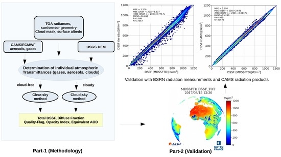
Satellite Retrieval of Downwelling Shortwave Surface Flux and Diffuse Fraction under All Sky Conditions in the Framework of the LSA SAF Program (Part 2: Evaluation)

Abstract

High frequency knowledge of the spatio-temporal distribution of the downwelling surface shortwave flux (DSSF) and its diffuse fraction (fd) at the surface is nowadays essential for understanding climate processes at the surface–atmosphere interface, plant photosynthesis and carbon cycle, and for the solar energy sector. The European Organization for the Exploitation of Meteorological Satellites (EUMETSAT) Satellite Application Facility for Land Surface Analysis operationally delivers estimation of the MDSSFTD (MSG Downwelling Surface Short-wave radiation Fluxes—Total and Diffuse fraction) product with an operational status since the year 2019. The method for retrieval was presented in a companion paper. Part 2 now focuses on the evaluation of the MDSSFTD algorithm and presents a comparison of the corresponding outputs, i.e., total DSSF and diffuse fraction (fd) components, against in situ measurements acquired at four Baseline Surface Radiation Network (BSRN) stations over a seven-month period. The validation is performed on an instantaneous basis. We show that the satellite estimates of DSSF and fd meet the target requirements defined by the user community for all-sky (clear and cloudy) conditions. For DSSF, the requirements are 20 Wm⁻² for DSSF < 200 Wm⁻², and 10% for DSSF ≥ 200 Wm⁻². The mean bias error (MBE) and relative mean bias error (rMBE) compared to the ground measurements are 3.618 Wm⁻² and 0.252%, respectively. For fd, the requirements are 0.1 for fd < 0.5, and 20% for fd ≥ 0.5. The MBE and rMBE compared to the ground measurements are −0.044% and −17.699%, respectively. The study also provides a separate analysis of the product performances for clear sky and cloudy sky conditions. The importance of representing the cloud–aerosol radiative coupling in the MDSSFTD method is discussed. Finally, it is concluded that the quality of the aerosol optical depth (AOD) forecasts currently available is accurate enough to obtain reliable diffuse solar flux estimates. This quality of AOD forecasts was still a limitation a few years ago.

1. Introduction

Downwelling surface short-wave radiation flux (DSSF) refers to the radiative energy, in the wavelength interval from 0.3 to 4.0 μm, reaching the Earth’s surface per time and area unit. An accurate knowledge of the spatio-temporal distribution of downwelling solar radiation at the surface is essential not only for understanding climate processes at the surface–atmosphere interface [1,2] but also for plant photosynthesis and the carbon cycle, e.g., [3,4,5], and for the solar energy sector [6]. Concerning the current status of DSSF modelling in atmospheric models, [7] and [8] found that the National Centers for Atmospheric Prediction (NCEP) and the National Center for Atmospheric Research (NCAR) data consistently overestimated DSSF by 17% to 27%. Comparisons with satellite data have also revealed large positive biases in NCEP–NCAR DSSF ranging from 25 to 50 Wm⁻² over the United States [9,10] and from 40 to 80 Wm⁻² over Europe [11]. However, in a recent study, [12] examined the progress made by two new reanalyses in the estimation of surface irradiance (ERA5 and COSMO-REA6) with negative biases of around −5 Wm⁻². They showed the largest deviations were found under clear sky conditions, which is most likely caused by the aerosol data used.

DSSF essentially depends on the solar zenith angle, cloud coverage, aerosols, and, to a lesser extent, on atmospheric absorption and surface albedo. Over the past few decades, the scientific community has developed computation methods to estimate both downward and net surface solar irradiance from satellite observations [13,14,15,16,17,18,19,20,21,22,23,24,25,26,27,28,29]. In addition to those estimates, two incoming solar radiation products derived from measurements of the SEVIRI sensor onboard Meteosat Second Generation (MSG) were also developed, being operated since 2005 by the European Organization for the Exploitation of Meteorological Satellites (EUMETSAT) Satellite Application Facility (SAF) on Land Surface Analysis (LSA; [30]): The MSG downwelling surface shortwave flux (MDSSF) product (referenced LSA-201) corresponds to instantaneous values and the DIDSSF product (LSA-203) corresponds to daily accumulated values. Both products consider clear and cloudy skies to provide total shortwave fluxes at the surface. However, all these estimates lack the repartition of the total flux into its direct and diffuse components (through the diffuse fraction, for example). Moreover, even though these products have proven to be of high quality, [31,32,33] showed that they still have some limitations under clear sky conditions, especially as they are determined by taking as hypothesis a temporally and spatially constant load and type of continental aerosols [34]. The importance of aerosols on the DSSF has been established in numerous studies on some highly polluted regions [35,36,37,38,39]. Thus, an initiative has been conducted by EUMETSAT to upgrade the physics in the scientific algorithms used for the satellite-derived DSSF retrievals and to provide first estimations of the diffuse fraction of the radiation.

The physics of this upgraded algorithm are described in a companion paper [40]. The new product version has been referenced as LSA-207 by EUMETSAT, corresponding to the MSG downwelling surface short-wave radiation fluxes total and diffuse fraction (MDSSFTD). Two different modules are used to calculate the set of MDSSFTD outputs, one for clear conditions and the other for cloudy conditions. The two methods are designed to ensure the spatial and temporal continuity of DSSF and diffuse fraction in the LSA-207 product. Details on the methodology as well as the major limitations are given in [40]. The input cloud mask is used to distinguish between the two methods. The summary of the two methods is as follows and is described in details in [40].

In clear sky conditions, the formulation based on the algorithm SIRAMix [41,42] is used to estimate the total flux and diffuse fraction. The atmospheric pressure, water content, ozone content and aerosols vary in time and space and are provided by atmospheric model forecasts. Both direct and diffuse flux terms are estimated by combining pre-computed aerosol transmittances and albedo (computed using radiative transfer models for varying aerosol load, solar zenith angles and water vapor content) from look-up tables and semi-empirical radiative transfer equations [42]. The total flux is the sum of both direct and diffuse flux estimates. The diffuse fraction is obtained as the ratio of the diffuse flux to the total flux estimate. In cloudy sky conditions, the total flux is estimated using simplified radiative transfer equations as described in [40]. The cloud transmittances are estimated from SEVIRI radiances at the top-of-atmosphere (TOA) level. The atmospheric transmittance term used for the estimation of the effective transmittance remains the same as in clear sky conditions. However, an extra cloud transmittance term is added as well as two multiple scattering terms. In the case of cloudy sky conditions, the diffuse fraction is estimated using an empirical formulation. The clear sky and cloudy sky methods are designed to provide smooth transitions in the frontiers between clear and cloudy pixels (see [40]). Finally, LSA-207 then includes an estimation of the total incoming solar radiation with an improved modelling of the aerosol impact on the atmospheric transmittance compared to the previous MDSSF product (LSA-201). The diffuse fraction of the radiation for all sky conditions is now also available. Moreover, estimations of auxiliary quantities are also provided: The equivalent aerosol optical depth (AOD) at 550 nm, the opacity index (OI) characterizing the opacity of the atmosphere (defined in [40]), and a quality flag information (QF).

This study evaluates the satellite-derived MDSSFTD product. The article is organized as follows: Section 2 presents the data and the metrics used for the validation; Section 3 presents the validation results; and Section 4 provides conclusions about the performance of the product regarding the user requirements.

2. Data and Metrics

2.1. Requirements

Over India, a satellite-based surface solar radiation dataset called Surface Solar Radiation Data Set-Heliosat (SARAH-E) was developed and evaluated against in situ measurements over a variety of sites. The results indicate an overestimation of the satellite DSSF, with a mean bias of 21.9 Wm⁻² [43]. A study over Finland and Sweden [44] also discussed the retrieval accuracies of two different satellite-derived DSSF datasets (the polar-orbiting satellite-based dataset, CLARA-A1, and the geostationary satellite-based dataset, SARAH). They showed comparable accuracies in comparison with ground measurements, in particular 10 Wm⁻² for the monthly means metrics and 15 Wm⁻² for daily means metrics. Over Europe, [31] completed an inter-comparison of satellite-derived incoming solar products from the different satellite application facilities of EUMETSAT and concluded that the products have comparable mean biases (+4 Wm⁻²) and root mean square differences (80–100 Wm⁻²) for instantaneous metrics. Performances of the historical LSA-SAF DSSF (LSA-201) satellite-derived incoming solar radiation product were also discussed in more detail in [45,46]. On an instantaneous basis, the bias between the satellite product and the ground data was shown to be small, with absolute values of less than 10 Wm⁻² over Europe [45], and even lower over France (3.75 Wm⁻² representing 2.5%). The standard deviation of the difference between instantaneous satellite estimates and ground measurements were of the order of 40 Wm⁻² for clear sky data and 110 Wm⁻² for cloudy sky data. Finally, the satellite estimates of DSSF are today ranging on average from 10 to 30 Wm⁻² in the absolute bias scale. However, these past works also pointed out that the absolute metrics usually used to evaluate the product performances are not equivalent if the domain (or period) of interest is located in high latitudes or low latitudes (or winter and summer periods).

The characteristics of the LSA-207 MDSSFTD product and the targeted accuracies agreed with EUMETSAT are described in

Table 1. Product requirements for MDSSFTD, in terms of area coverage, resolution, and accuracy. The targeted requirements are indicated in bold.

Product	Coverage	Resolution		Accuracy
		Temporal	Spatial	Threshold	Target	Optimal
MDSSFTD (LSA-207) DSSF	MSG disk	15 min	MSG pixel resolution	20%	DSSF < 200 W/m2: 20 W/m2 (MBE) DSSF ≥ 200 W/m2: 10% (rMBE)	5%
MDSSFTD (LSA-207) FRACTION_DIFFUSE (fd)	MSG disk	15 min	MSG pixel resolution	30%	fd < 0.5: 0.1 (MBE) fd ≥ 0.5: 20% (rMBE)	10%

. They are a compromise between what is currently achievable, given existing observations and algorithm input data, and what would suit most users and applications. In this respect, the ‘threshold’ requirement is then defined as the minimum accuracy that is acceptable for DSSF user needs. This paper assesses the performance of the product by referring to the ‘target’ requirement. However, it may be relevant to note that because the topic of the retrieval of diffuse fraction from satellites is very recent, today, no performance requirements are defined by the scientific community for this parameter. We therefore fixed the ‘target’ accuracy to 20%, although a larger uncertainty (e.g., >30%) could have also been considered. The target accuracy metrics used are the mean bias error (MBE) for low values, and the relative MBE (rMBE) for high values of DSSF or fd.

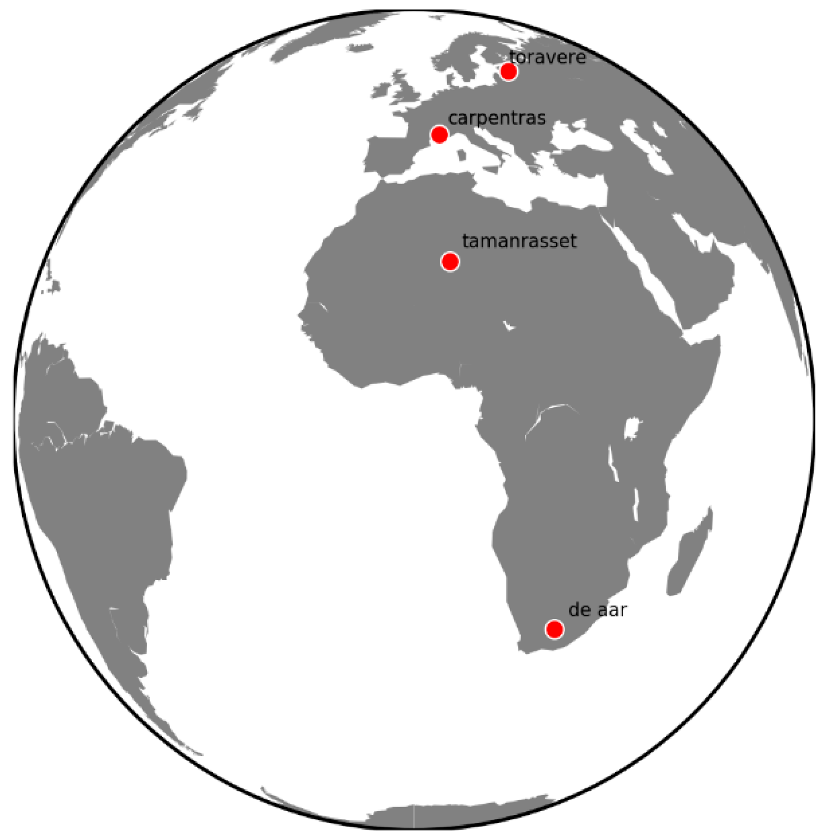
2.2. Ground Measurements and Preprocessing

Four ground stations were used for the validation analyses presented in this document. The stations considered are Carpentras, De Aar, Tamanrasset, and Toravere from the BSRN (Baseline Surface Radiation Network, http://www.bsrn.awi.de) of the World Climate Research Program. Their location is presented in Figure 1.

The in situ measurements of instantaneous total and diffuse DSSF as observed at these stations were used as a reference. The stations are located in climatically different regions of Europe and Africa. For example, the station Tamanrasset in North Africa is influenced by coarser dust particles and more clear conditions than the other Europe-based stations. Toravere is located at the highest latitude and therefore is related to frequent periods of overcast in the winter and fall. This will help evaluate the MDSSFTD method under cloudy situations and high solar zenith angles.

BSRN-derived surface flux values are retrieved at a high temporal frequency going from 1 min to a few minutes. BSRN data already account for missing or bad measurements for which missing flag values are assigned. The missing values are discarded in the comparison with satellite flux measurements. The direct flux measurements account for the varying solar zenith angle dependence. All measurements (total, diffuse, and direct surface solar flux measurements) are discarded when the solar zenith angle is greater than 80 degrees. MSG/SEVIRI satellite-derived products differ on a pixel basis from 0 to 12 min with the product time. The SEVIRI scan takes 12 min for the data acquisition over the MSG disk starting from the south pole and finishing its acquisition in the north pole. For the sake of a fair comparison, the ground measurements were averaged over 15 min, centered around the exact acquisition time of the satellite for every SEVIRI pixel. The relationship between the estimated time difference as a function of row number (or latitude) is detailed in other LSA SAF reports (product user manual MDSSF; 2.6V2 at https://landsaf.ipma.pt/en/products/longwave-shortwave-radiation/; last time consulted on 2 September 2019). Note that the diffuse fraction is not a direct measurement. This variable is obtained by dividing the diffuse component over the total component, which are measured by the ground instruments. The BSRN total fluxes and diffuse fluxes are measured respectively with pyranometers and shaded pyranometers (Kipp & Zonen/CM21 for stations Carpentras and Toravere, Kipp & Zonen/CMP21 for station De Aar, and Eppley/PSP for station Tamanrasset). The accuracy of the BSRN total fluxes measurements, provided the measure is made according to the BSRN protocol, is estimated to 0.5% or 1.5 Wm⁻², while the accuracy of the diffuse measurements is estimated to 2% or 3 Wm⁻² [47]. In practice, specific analyses on BSRN sites’ accuracy [48,49] confirmed that the uncertainty of the measures is in agreement with such levels of uncertainties, with some limitations for low sun elevation angles and low radiation fluxes. As the validity of the MDSSFTD products is limited to sun zenith angles below 80°, we consider that the in situ measurement of total fluxes and the BSRN-derived diffuse fractions can reasonably be taken as references for our validation analysis.

2.3. CAMS All-Sky Radiation Data

The Copernicus Atmosphere Monitoring Service (CAMS) all-sky radiation data were also used for comparison with the MDSSFTD product. CAMS all-sky radiation service distributes global, direct and diffuse irradiances as well as a direct at normal incidence irradiance, for all sky (clear + cloud), clear sky only, and cloudy sky only. These data are provided as timeseries with a temporal resolution of 1 min, 15 min, 1 h, 1 day, or 1 month, and are made available since February 2004 with a 2-day delay. The spatial coverage corresponds to the Meteosat Second Generation (MSG) disk. To produce the timeseries, radiation data were spatially interpolated to the point of interest from a product available at the native spatial resolution of MSG/SEVIRI. These data are publicly available from the CAMS portal (https://atmosphere.copernicus.eu/solar-radiation, last consulted on 18/10/2019).

The CAMS Radiation service relies on the Heliosat-4 method [50], which is composed of two modules: McClear v3 for clear skies [51,52] and McCloud for cloudy skies [50]. The McClear approach, version 3, used by the CAMS radiation service, has been upgraded from McClear v2 and now consists of physical modelling using the radiative transfer model libRadtran [53]. As for the MDSSFTD method, the McClear v3 also now relies on aerosol content and load, as well as gas contents forecasted by ECMWF and distributed by CAMS. Compared to the MDSSFTD method, McClear v3 uses a monthly climatology [54] of the MODIS surface albedos [55] and a similar approach to MDSSFTD for the aggregation of the optical depths of each aerosol species to derive the properties of the aerosol mixture [52]. The McCloud method estimates the cloud properties from MSG measurements using a model adapted from APOLLO (AVHRR Processing scheme Over cLouds, Land, and Ocean, [56,57]).

For our validation analysis, we used the CAMS global and diffuse radiation data, at a temporal resolution of 15 min. For the sake of consistency with the evaluation against ground measurements, the product was extracted for the whole validation period (February to October 2017) at the location of the four BSRN stations already considered for the ground measurement analysis (Carpentras, De Aar, Tamanrasset and Toravere).

2.4. Metrics

The target accuracy metrics used were the mean bias error (MBE) for low values of DSSF (<200 Wm⁻²) or fd (<0.5). The target accuracy metrics used are the relative MBE (rMBE) for high values of DSSF (≥200 Wm⁻²) or fd (≥0.5). MBE was computed as:

$$MBE=\frac{1}{N}{{\displaystyle \sum }}_{i=1}^N\left(satelliteproduc{t}_i-referenc{e}_i\right),$$

(1)

and the relative MBE, noted “rMBE”, is a dimensionless metric, expressed in percent units, and defined as:

$$rMBE=\frac{1}{N}{{\displaystyle \sum }}_{i=1}^N\frac{satelliteproduc{t}_i-referenc{e}_i}{referenc{e}_i},$$

(2)

where N is the number of points and ‘reference’ corresponds to the ground measurements in our study.

The choice of the metrics was made to ensure consistency with the two other existing LSA-SAF products MDSSF and DIDSSF (LSA-201 and 203; see Section 1), for which the same evaluation strategy was used. The ground measurements were separated into clear and cloudy samples based on the information contained in the cloud mask. For example, if the SEVIRI pixel was defined as cloudy (respectively clear) according to the information contained in the quality flag, the corresponding time slot was then defined as cloudy (respectively clear) for the ground measurements. In the case of clear sky retrievals, the clear sky pixel was excluded when the adjacent time slots (up to 1 h, that is, 30 min before and 30 min after) were defined as cloudy. This is deemed to suppress any residual cloud contamination (or cloud shadow effects) in the clear sky retrievals. The same strategy was applied reversely to identify cloudy sky pixels with adjacent time slots that were clear sky.

The requirements were the target accuracies (values in bold Table 1). These metrics will be used in the following section to evaluate the performances of the MDSSFTD product for clear sky, cloudy sky, and all sky conditions. However, the user need expressed to EUMETSAT is to have a MDSSFTD product that meets the target requirements for the all sky conditions (without distinction according to cloudiness). The performances were evaluated based on the metrics that were obtained from all the available ground measurements (i.e., for all stations and over the entire period of evaluation). The MDSSFTD product has the spatial resolution of the native SEVIRI grid (3 km at the sub-satellite point over Africa and around 5 km over Europe). The authors of Hakuba et al. [58] showed that there is no major representativeness issue between the local ground-based solar radiation measurements and the satellite estimates (which have kilometer scales).

The evaluation was performed over a period of seven months from February to October 2017. The stability of the metrics was also examined by splitting the metrics on a daily basis and analyzing the stability of the metrics from day to day.

3. Results

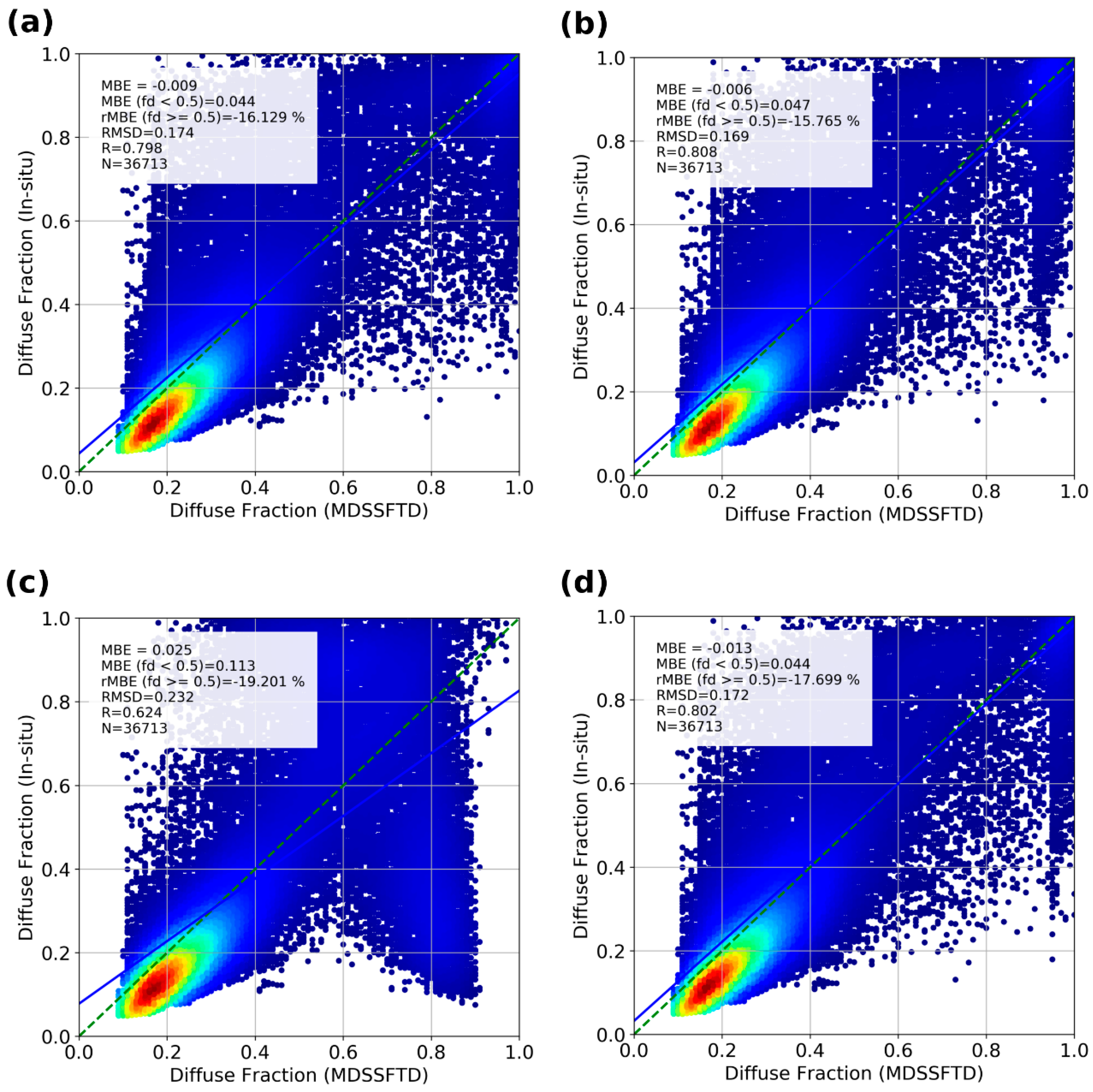
3.1. Sensitivity Study: Inter-Comparison of Models to Estimate Diffuse Flux in Cloudy Sky Conditions

A critical module in the method used for MDSSFTD is the choice of the empirical formulation used to estimate the diffuse fraction in the cloudy sky case. In this context, a specific sensitivity study was first made to compare a set of existing solutions. One shall note that this sensitivity study only reflects the impact of the parametrization choice on the diffuse fraction retrieval under cloudy conditions. Retrieval of the diffuse fraction under a clear sky remains unchanged (see [40]).

We detail here this sensitivity study that compared several empirical formulations from the literature. The different formulations were based on [59,60,61]. All three methods estimate the diffuse part of the total solar irradiance from the clearness index (‘Kt’). This allows the calculation of the diffuse fraction by simply dividing the diffuse flux by the total counterpart. Another formulation based on [62] was also considered in this sensitivity study. This fourth method, however, estimates the direct component of the solar irradiance based on ‘Kt’, which is used to infer the direct fraction of the solar irradiance to finally retrieve the diffuse fraction.

Figure 2 displays the density scatter plots for the diffuse fraction retrieved following each of the four formulations mentioned above, all compared to the in situ diffuse fraction in all sky conditions (clear and cloudy). The statistics shown in Figure 2 were obtained considering the four stations over the entire period of the study. As can be seen, the statistics from the four formulations are highly similar, with slightly lower performances for the method from [62]. Because the formulation based on [60] was validated against several stations over Europe and the USA, we decided to use this formulation for our application. Indeed, the other models were derived from flux measurements over more limited areas, which make them less representative at the continental scale made possible by MSG.

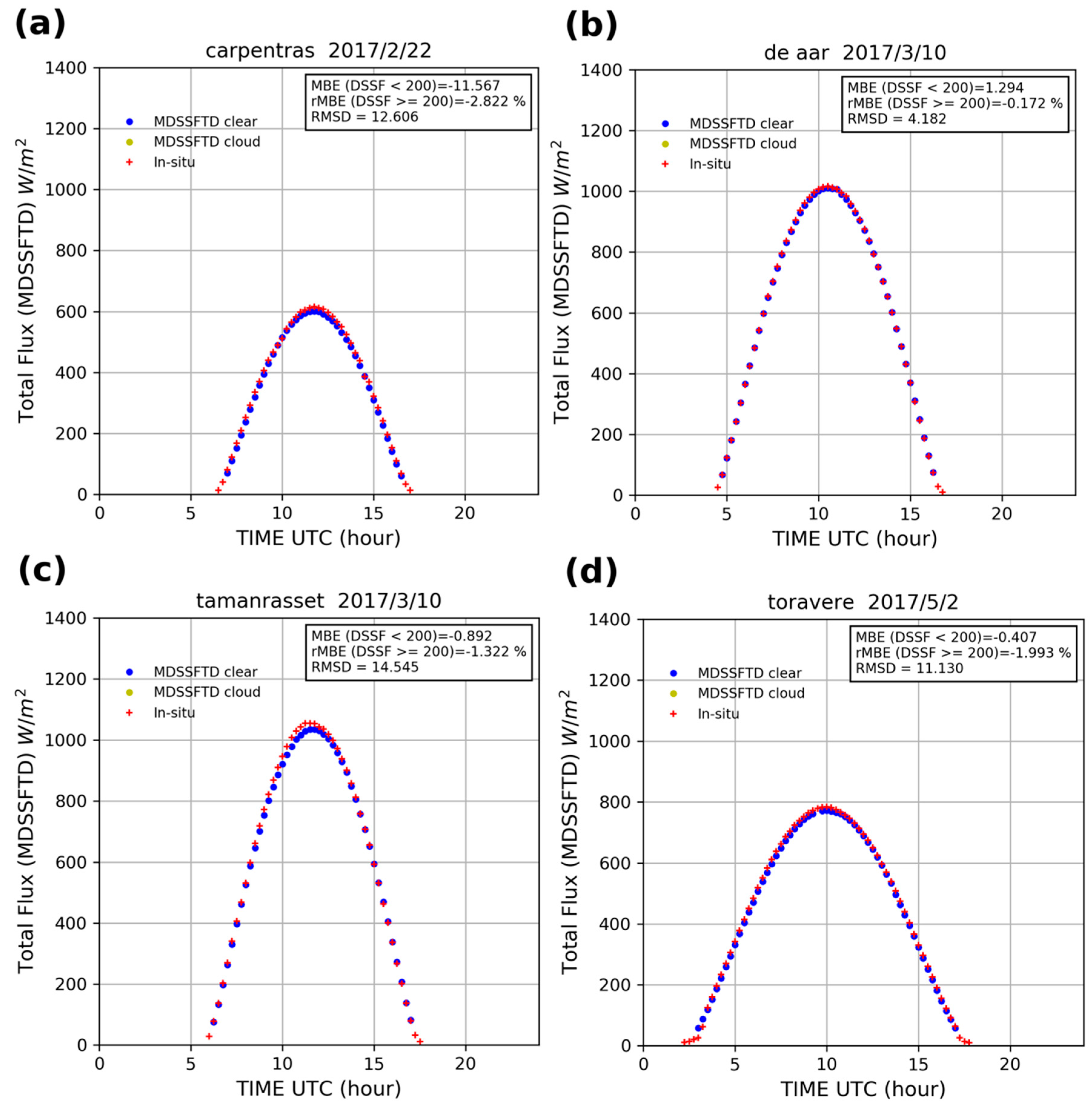
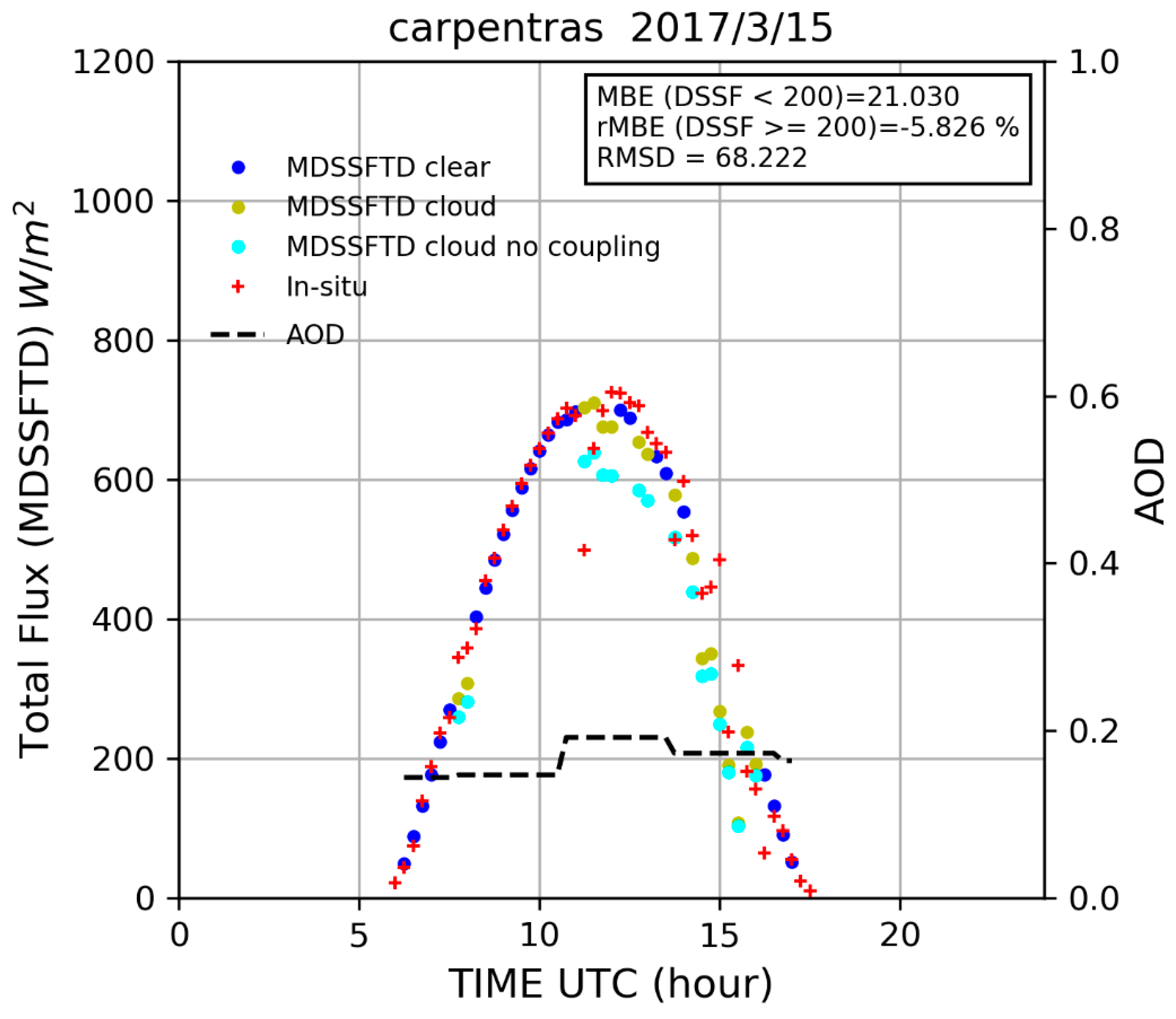
3.2. Diurnal Comparisons for Clear Sky and All Sky Days

The diurnal total and diffuse downwelling surface flux components from the MDSSFTD product were compared against the same flux components derived from the ground BSRN measurements. As already mentioned, the BSRN data (available at a high temporal frequency) were averaged over 15 min and centered around the correct MSG acquisition time slot (see Section 2.2).

Figure 3 shows a comparison between satellite-derived estimates and ground measurements of the diurnal cycle of the total flux for clear sky conditions over the day. It can be observed how the satellite-derived estimates capture the diurnal variations well compared to the ground measurements.

Figure 4 shows a comparison between satellite-derived estimates and ground measurements of the diurnal cycle of the diffuse fraction for clear sky conditions. Again, the satellite-derived estimates capture the diurnal variations well compared to the ground measurements. In particular, the increase of the diffuse fraction with extreme geometries is reproduced well. For these four days, a slight overestimation between 0.055 and 0.142 was found for fd < 0.5 in clear sky conditions. This overestimation comes from the slight overestimation of the diffuse DSSF by MDSSFTD, which was also found for clear sky situations by [41] when using SIRAMix and the McClear method [51]. These two methods used CAMS aerosol data and GADS aerosol properties, which may point to an overestimation of the highly scattering aerosol components by CAMS or a limited transformation from CAMS to GADS components.

Figure 5 and Figure 6 show the results of similar comparisons that were conducted for dates showing all sky conditions (partially clear and partially cloudy). The diurnal variations of the MDSSFTD product, including the total DSSF and diffuse fraction, are compared against ground measurements for selected days in Figure 5 and Figure 6, respectively. A rather satisfactory agreement exists between the satellite-derived estimates and the ground measurements. The increase of the diffuse fraction with the cloudiness is generally well represented (e.g., see Figure 6d).

3.3. Global Performances

This section details the overall statistics of the MDSSFTD product that were obtained by considering the evaluation over the four ground stations for the entire period of interest, with a temporal frequency of 15 min. The statistics are hence discussed successively for clear sky, cloudy sky, and all sky conditions.

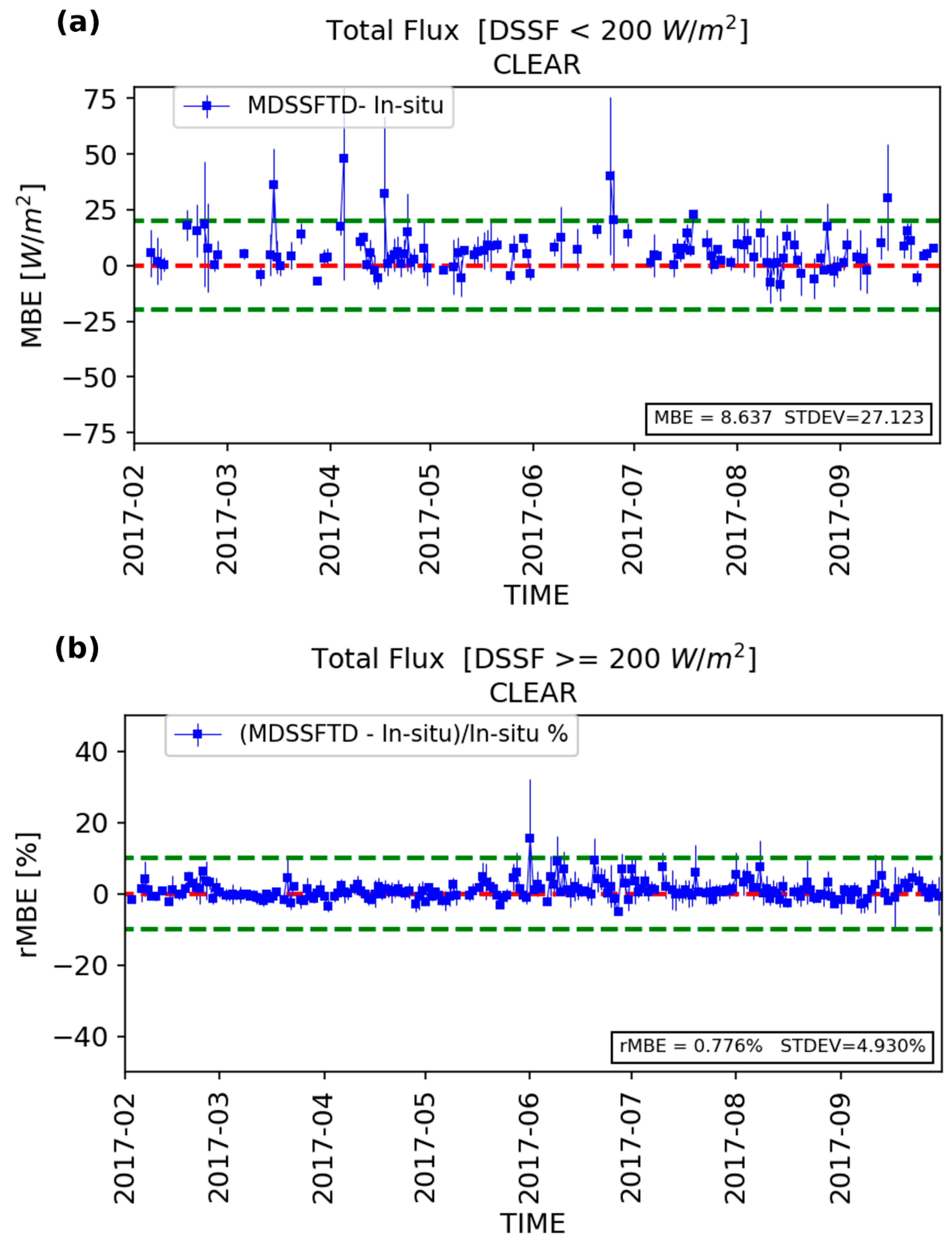
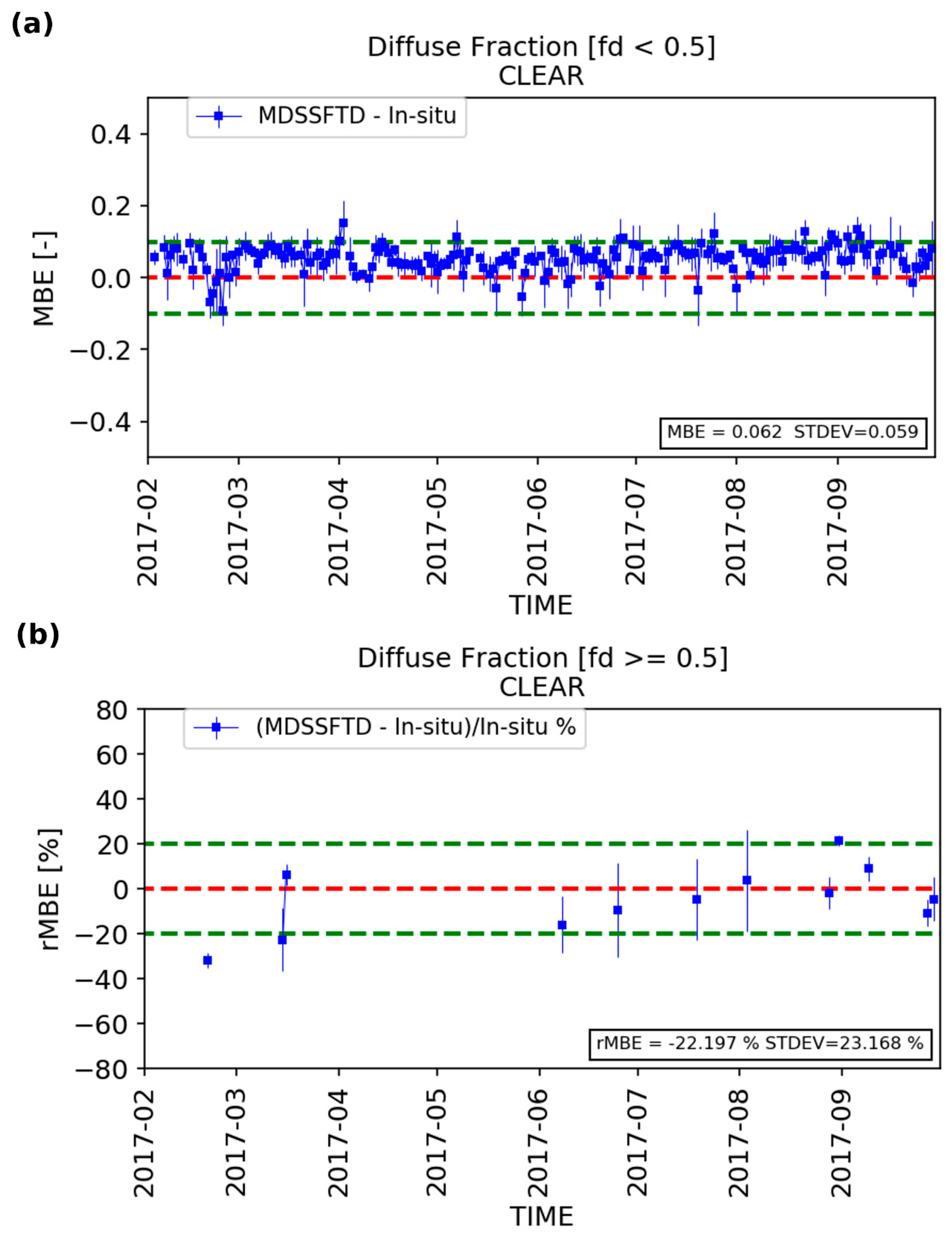
3.3.1. Clear Sky Conditions

Figure 7 displays the density scatter plot between the instantaneous measurements of MSG-derived surface downwelling solar flux measurements for total and diffuse fraction components with their in situ counterparts. Only clear sky retrievals are considered here thanks to the use of the cloud mask used as input in the MDSSFTD algorithm. Figure 7 shows that the satellite estimates of DSSF and fd meet the requirements for total DSSF, which are 20 Wm⁻² for DSSF < 200 Wm⁻² and 10% for DSSF ≥ 200 Wm⁻² (as described in Table 1). The MBE and rMBE compared to the ground measurements are 8.637 Wm⁻² and 0.776%, respectively. On the other hand, the requirements for fd are 0.1 for fd < 0.5 and 20% for fd ≥ 0.5. The MBE and rMBE compared to the ground measurements in this case are 0.062% and −22.197%, respectively. The statistical scores in terms of MBE and RMSD (root mean square deviation) for the comparison between MDSSFTD total and diffuse fraction components with their in situ counterparts for all four stations are given in

Table 2. Statistical scores obtained from the comparison between MDSSFTD-derived total flux estimates and ground in situ measurements over the selected BSRN sites for clear sky retrievals. If the value is in bold, the metric does not meet the “target” requirements. If no value appears in bold, all the metrics meet the requirements. R_VAL corresponds to the Pearson correlation coefficient. RMSD is the root mean square deviation.

	Lat (°N)	Lon (°E)	R_VAL (-)	RMSD (Wm−2)	MBE (Wm−2)	MBE (DSSF < 200) (Wm−2)	rMBE (DSSF ≥ 200) (%)
Carpentras	44.08	5.06	0.998	22.809	14.552	6.759	2.623
De Aar	−30.67	23.99	0.996	23.042	−2.946	8.927	−0.797
Tamanrasset	22.79	5.53	0.995	34.096	−0.441	12.336	0.798
Toravere	58.25	26.46	0.996	19.277	1.488	4.297	0.320

and

Table 3. Statistical scores obtained from the comparison between MDSSFTD diffuse fraction estimates and ground measurements over the selected BSRN sites for clear sky retrievals. If the value is in bold, the metric does not meet the “target” requirements. If no value appears in bold, all the metrics meet the requirements. R_VAL corresponds to the Pearson correlation coefficient. RMSD is the root mean square deviation.

	Lat (°N)	Lon (°E)	R_VAL (-)	RMSD (-)	MBE (-)	MBE (fd < 0.5) (-)	rMBE (fd ≥ 0.5) (%)
Carpentras	44.08	5.06	0.890	0.069	0.042	0.045	−10.173
De Aar	−30.67	23.99	0.624	0.115	0.065	0.073	−47.698
Tamanrasset	22.79	5.53	0.831	0.134	0.028	0.072	−21.216
Toravere	58.25	26.46	0.768	0.091	0.027	0.039	−31.354

. The scores for all stations are in agreement with the DSSF product requirements. The diffuse fraction compares well for all stations except for high values of diffuse fraction (fd ≥ 0.5). However, only 12 days over the 7-month period of the study have fd ≥ 0.5 in clear sky conditions (see Figure 13). Indeed, these values of diffuse fraction correspond to intense aerosol loading, which is relatively infrequent. Therefore, the statistics in that case (fd ≥ 0.5 and clear sky conditions) cannot be considered as significant from a statistical point of view.

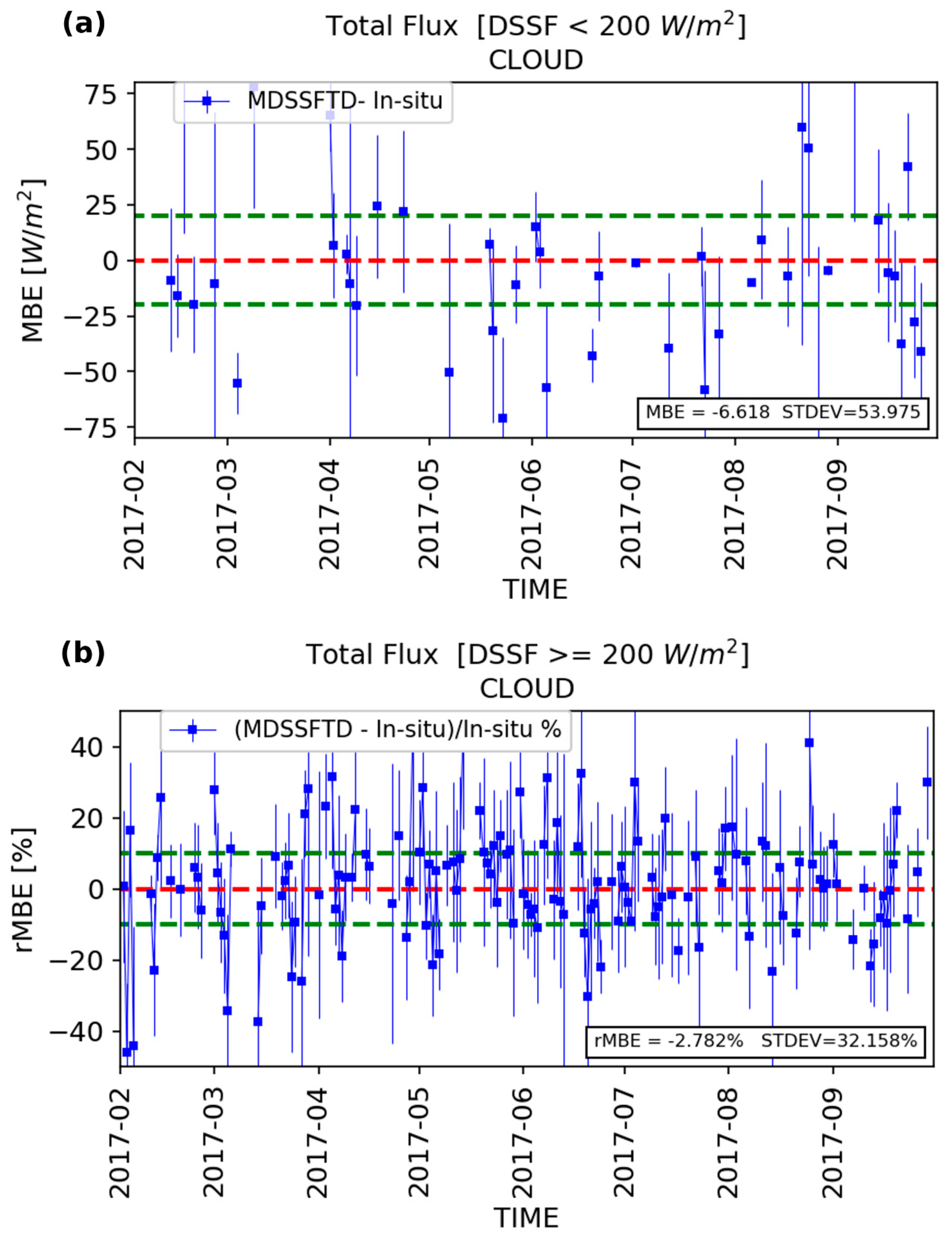
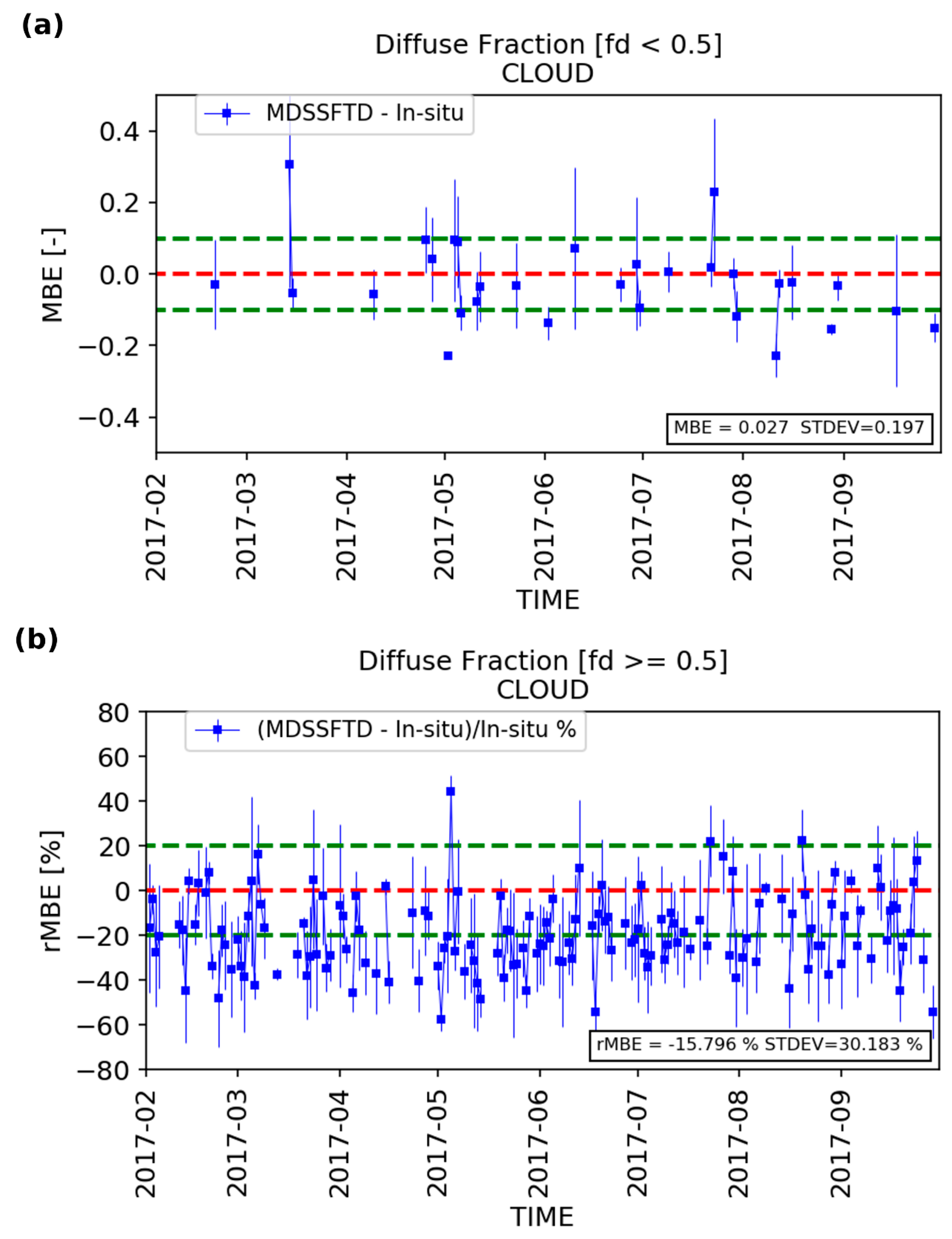
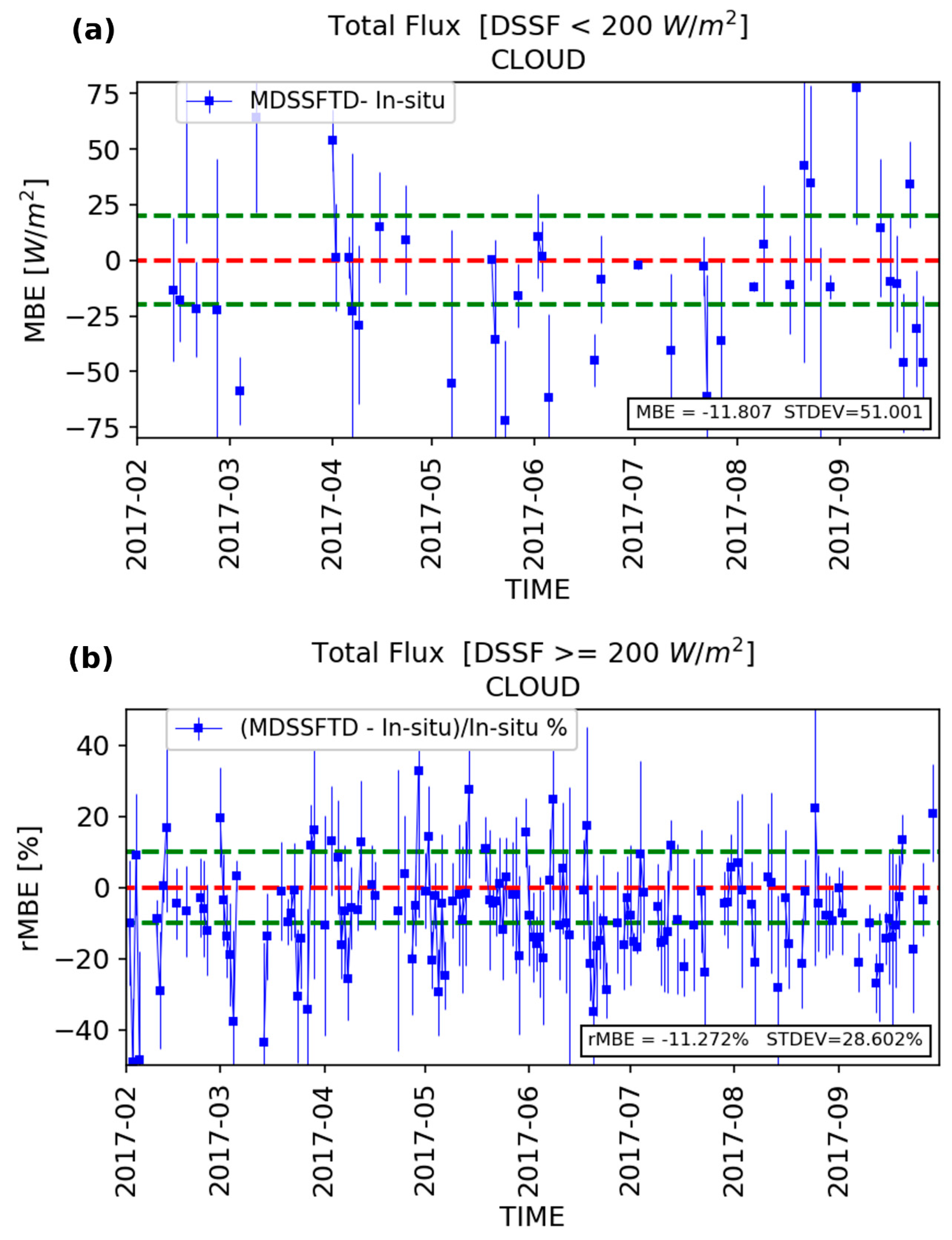
3.3.2. Cloudy Sky Conditions

Figure 8 displays the density scatter plot between instantaneous measurements of MSG-derived surface downwelling solar flux measurements for total and diffuse fraction components with their in situ counterparts. Only cloudy sky retrievals were considered for this experiment. Figure 8 shows that the satellite estimates of DSSF and fd meet the target requirements. For DSSF, the requirements are 20 Wm⁻² for DSSF < 200 Wm⁻² and 10% for DSSF ≥ 200 Wm⁻². The MBE and rMBE compared to the ground measurements are −6.618 Wm⁻² and −2.782%, respectively. For fd, the requirements are 0.1 for fd < 0.5 and 20% for fd ≥ 0.5. The MBE and rMBE compared to the ground measurements are 0.027% and −15.796%, respectively.

Table 4. Statistical scores obtained from the comparison between MDSSFTD total flux estimates and ground measurements over the selected BSRN sites for cloudy sky retrievals. If the value is in bold, the metric does not meet the “target” requirements. If no value appears in bold, all the metrics meet the requirements.

	Lat (°N)	Lon (°E)	R_VAL (-)	RMSD (Wm−2)	MBE (Wm−2)	MBE (DSSF < 200) (Wm−2)	rMBE (DSSF ≥ 200) (%)
Carpentras	44.08	5.06	0.886	124.089	−5.226	−20.663	−1.463
De Aar	−30.67	23.99	0.860	144.928	−22.573	−16.236	−5.585
Tamanrasset	22.79	5.53	0.861	174.924	54.220	−21.255	10.806
Toravere	58.25	26.46	0.880	117.562	−34.572	0.800	−8.025

and

Table 5. Statistical scores obtained from the comparison between MDSSFTD diffuse fraction estimates and ground measurements over the selected BSRN sites for cloudy sky retrievals. If the value is in bold, the metric does not meet the “target” requirements. If no value appears in bold, all the metrics meet the requirements.

	Lat (°N)	Lon (°E)	R_VAL (-)	RMSD (-)	MBE (-)	MBE (fd < 0.5) (-)	rMBE (fd ≥ 0.5) (%)
Carpentras	44.08	5.06	0.620	0.246	−0.108	−0.047	−15.082
De Aar	−30.67	23.99	0.489	0.287	−0.109	−0.007	−17.631
Tamanrasset	22.79	5.53	0.418	0.306	−0.198	−0.079	−25.767
Toravere	58.25	26.46	0.647	0.215	−0,060	0.064	−11.693

give the statistical scores in terms of MBE and RMSD for the comparison between the MDSSFTD total and diffuse fraction components with their in situ counterparts for all four stations. The vertical patterns that are observed in Figure 8b come from the method that is used for cloudy skies. Indeed, the estimation of the diffuse fraction was estimated using three equations that were selected according to the value of the clearness index. More details are given in the companion paper [40].

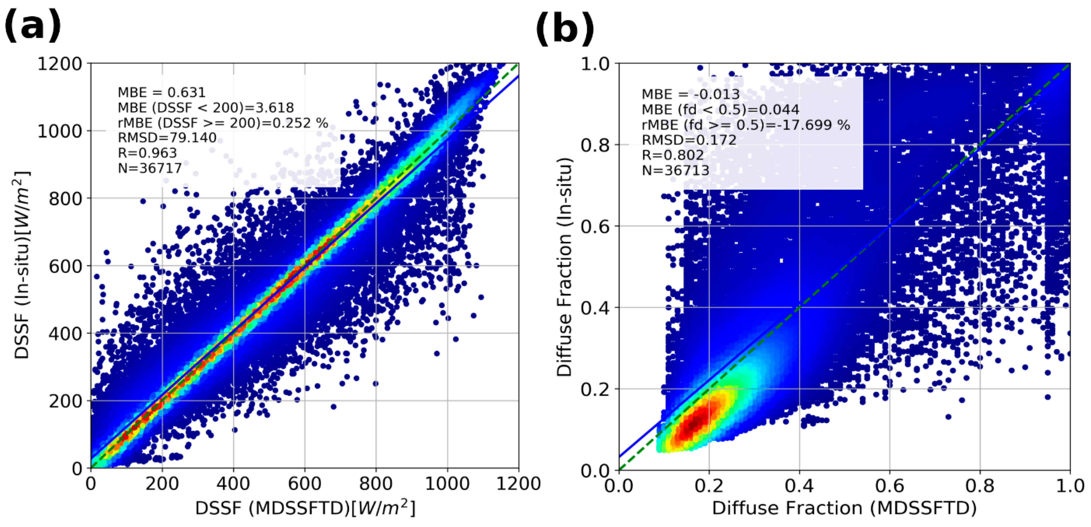
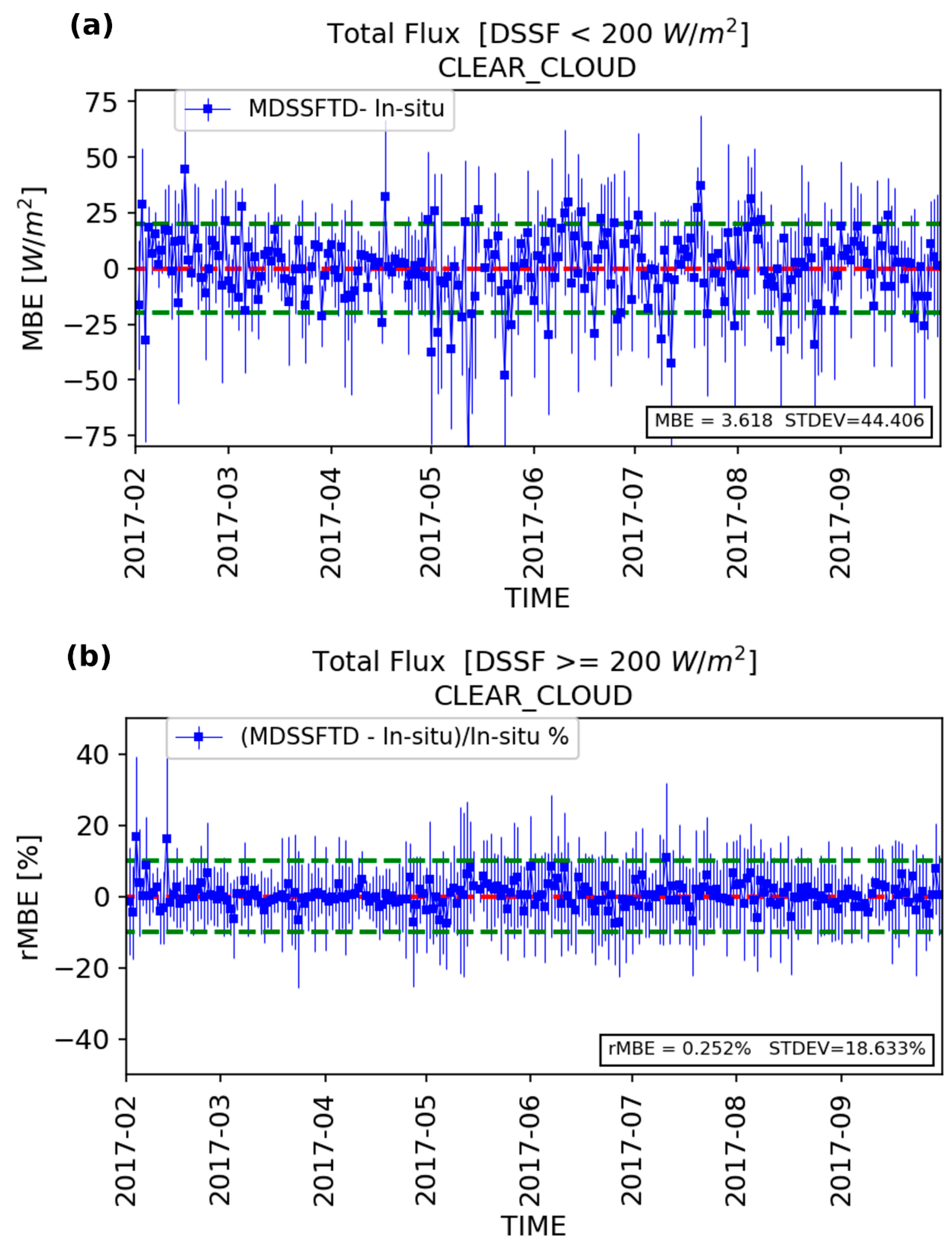
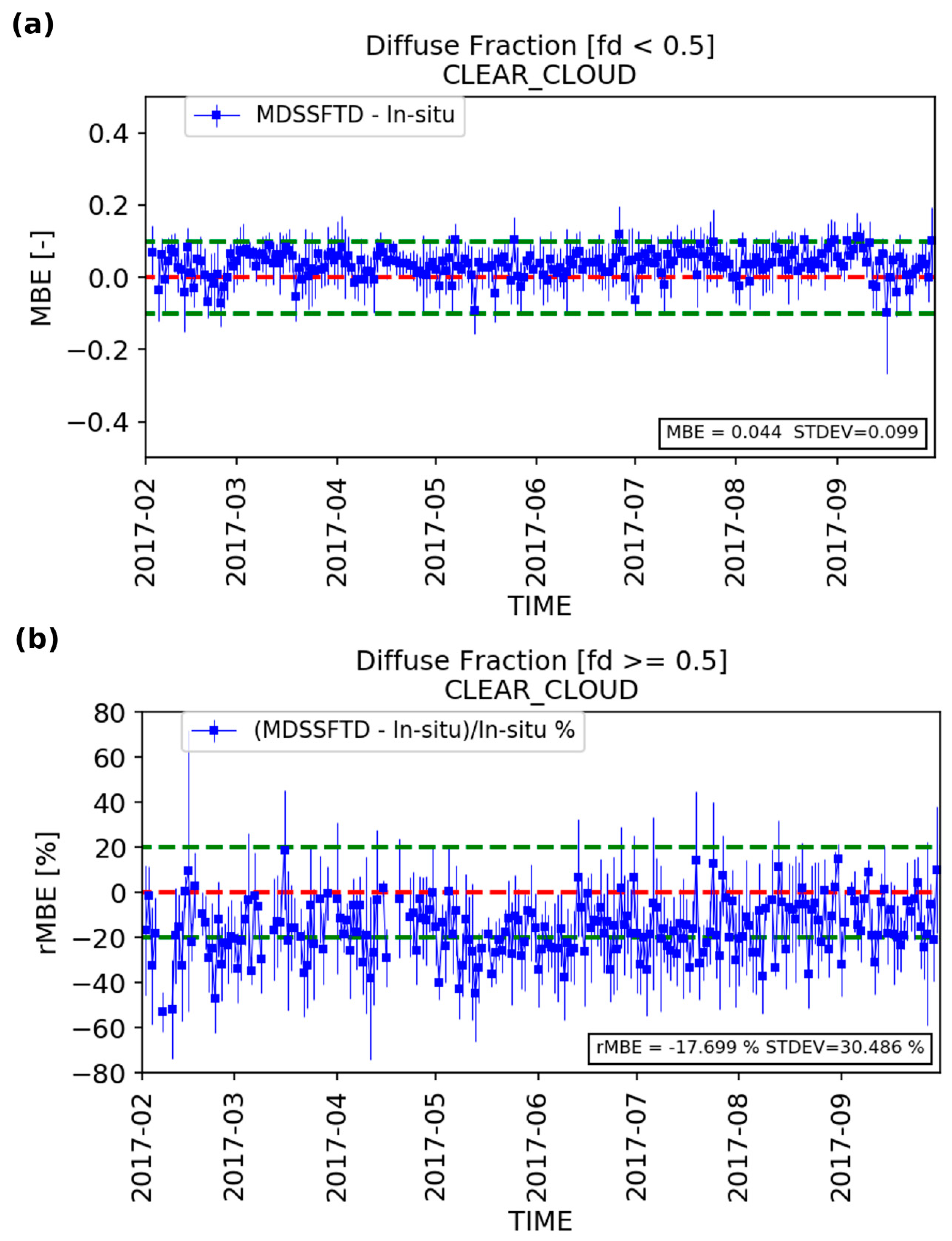
3.3.3. All Sky (Clear and Cloudy) Conditions

In a similar way, the total DSSF and diffuse fraction from the MDSSFTD product for all sky retrievals were compared against their in situ counterparts in Figure 9. Note that the metrics obtained for the all sky conditions are those that were used to evaluate the performances of the product in the framework of the LSA SAF program (see Section 2.4).

Figure 9 displays the density scatter plot between instantaneous measurements of MSG-derived surface downwelling solar flux measurements for total and diffuse fraction components with their in situ counterparts for the all sky retrievals. Figure 9 shows that the satellite estimates of DSSF and fd meet the requirements. For DSSF, the requirements are 20 Wm⁻² for DSSF < 200 Wm⁻² and 10% for DSSF ≥ 200 Wm⁻². The MBE and rMBE compared to the ground measurements are 3.618 Wm⁻² and 0.252%, respectively. For fd, the requirements are 0.1 for fd < 0.5 and 20% for fd ≥ 0.5 Wm⁻². The MBE and rMBE compared to the ground measurements are 0.044% and −17.699%, respectively. The statistical scores in terms of MBE and RMSD for the comparison between MDSSFTD total and diffuse fraction components with their in situ counterparts for all four stations are given in

Table 6. Statistical scores obtained from the comparison between MDSSFTD total flux estimates and ground measurements over the selected BSRN sites for all (clear and cloudy) sky retrievals. If the value is in bold, the metric does not meet the “target” requirements. If no value appears in bold, all the metrics meet the requirements.

	Lat (°N)	Lon (°E)	R_VAL (-)	RMSD (Wm−2)	MBE (Wm−2)	MBE (DSSF < 200) (Wm−2)	rMBE (DSSF ≥ 200) (%)
Carpentras	44.08	5.06	0.969	69.584	10.790	0.728	2.037
De Aar	−30.67	23.99	0.969	64.833	−4.015	5.891	−0.993
Tamanrasset	22.79	5.53	0.965	86.075	10.722	5.034	2.939
Toravere	58.25	26.46	0.917	94.607	−18.026	3.604	−4.125

and

Table 7. Statistical scores obtained from the comparison between MDSSFTD diffuse fraction estimates and ground measurements over the selected BSRN sites for all (clear and cloudy) sky retrievals. If the value is in bold, the metric does not meet the “target” requirements. If no value appears in bold, all the metrics meet the requirements.

	Lat (°N)	Lon (°E)	R_VAL (-)	RMSD (-)	MBE (-)	MBE (fd < 0.5) (-)	rMBE (fd ≥ 0.5) (%)
Carpentras	44.08	5.06	0.818	0.151	−0.006	0.029	−14.753
De Aar	−30.67	23.99	0.734	0.161	0.022	0.054	−21.809
Tamanrasset	22.79	5.53	0.755	0.184	−0.034	0.057	−22.949
Toravere	58.25	26.46	0.786	0.191	−0,035	0.038	−13.361

. The scores for all stations are in agreement with the MDSSFTD product requirements. The diffuse fraction compares well for most stations except in De Aar and Tamanrasset if a 20% threshold is considered for fd > 0.5.

3.4. Stability of the Metrics

Here, we present the time series of the mean statistics averaged over all stations for the MDSSFTD total flux products (DSSF and fd). The goal was to study the temporal evolution of performances with time. The 15-min statistics between the 15-min satellite-derived products and the 15-min resampled ground measurements were averaged on a daily basis. The standard deviations of the 15-min statistics were also calculated on a daily basis and are reported in the following plots. The statistics were calculated for both DSSF regimes and both outputs: For total flux, DSSF less than 200 Wm⁻² and greater than 200 Wm⁻²; and for the diffuse fraction, fd lower than 0.5 and greater than 0.5.

First, Figure 10, Figure 11 and Figure 12 show the time series of the metrics for DSSF under clear, cloudy, and all sky (clear and cloudy) conditions, respectively. Second, Figure 13, Figure 14 and Figure 15 show the time series of the metrics for diffuse fraction under clear, cloudy, and all sky (clear and cloudy) conditions, respectively. All figures show the daily averages along with the standard deviation, which is related to the variation of the values among the different stations. First, it is important to highlight that all these conditions do not have the same level of representativeness due to the varying number of samples in the different cases. The only case that frequently shows values going beyond the requirement limits (i.e., the horizontal green lines) is the cloudy sky case for high values of fd (fd ≥ 0.5; see Figure 14). In all the other conditions, and especially for all sky (clear and cloudy) conditions, the average statistics obtained from the product outputs meet the target requirement along the entire period of the analysis.

3.5. Impact of the Activation of the Cloud–Aerosol Coupling

The method for DSSF retrieval is using a simple radiative transfer model that takes into account the radiative coupling between aerosols and clouds as described in the Equation (24) of the companion paper [40] (see the fourth term of equation). Figure 16 gives an example of this cloud–aerosol coupling for a selected day in Carpentras. We clearly observe a better agreement with the in situ measurements around noon in the case of the activation of the cloud–aerosol radiative coupling (yellow dots compared to light blue dots). Even if the aerosol optical depth (AOD) is not large (i.e., 0.2), the impact of the cloud–aerosol coupling remains important. This may be due to the presence of very thin clouds in the high atmosphere.

Figure 11 has showed the performances of the DSSF estimated by the MDSSFTD algorithm, which considers the influence of the cloud–aerosol coupling under cloudy sky conditions. The MDSSFTD satellite estimates are very close to the in situ measurements (MBE = −6.618, rMBE = −2.782%). Figure 17 shows the same comparison using the same code after disabling the coupling between the cloud and aerosols (by simply removing the fourth term of Equation (24) in [40]). We can clearly observe a large degradation of the performances of the algorithm in this case (MBE = −11.807 Wm⁻², rMBE = −11.272%). The presence of aerosols makes the atmospheric transmittance decrease, and in turn the DSSF becomes lower. However, this atmospheric transmittance decrease is too large in cloudy conditions. This sensitivity test illustrates the importance of the indirect radiative impacts of clouds on aerosol radiative forcing. In our study, the activation of the coupling improves the performances by about 8%. Clouds induce an increase of the atmospheric transmittance by reflecting, back to the surface, part of the radiation scattered by aerosols. This radiative cloud–aerosol coupling is included in the LSA-207 product.

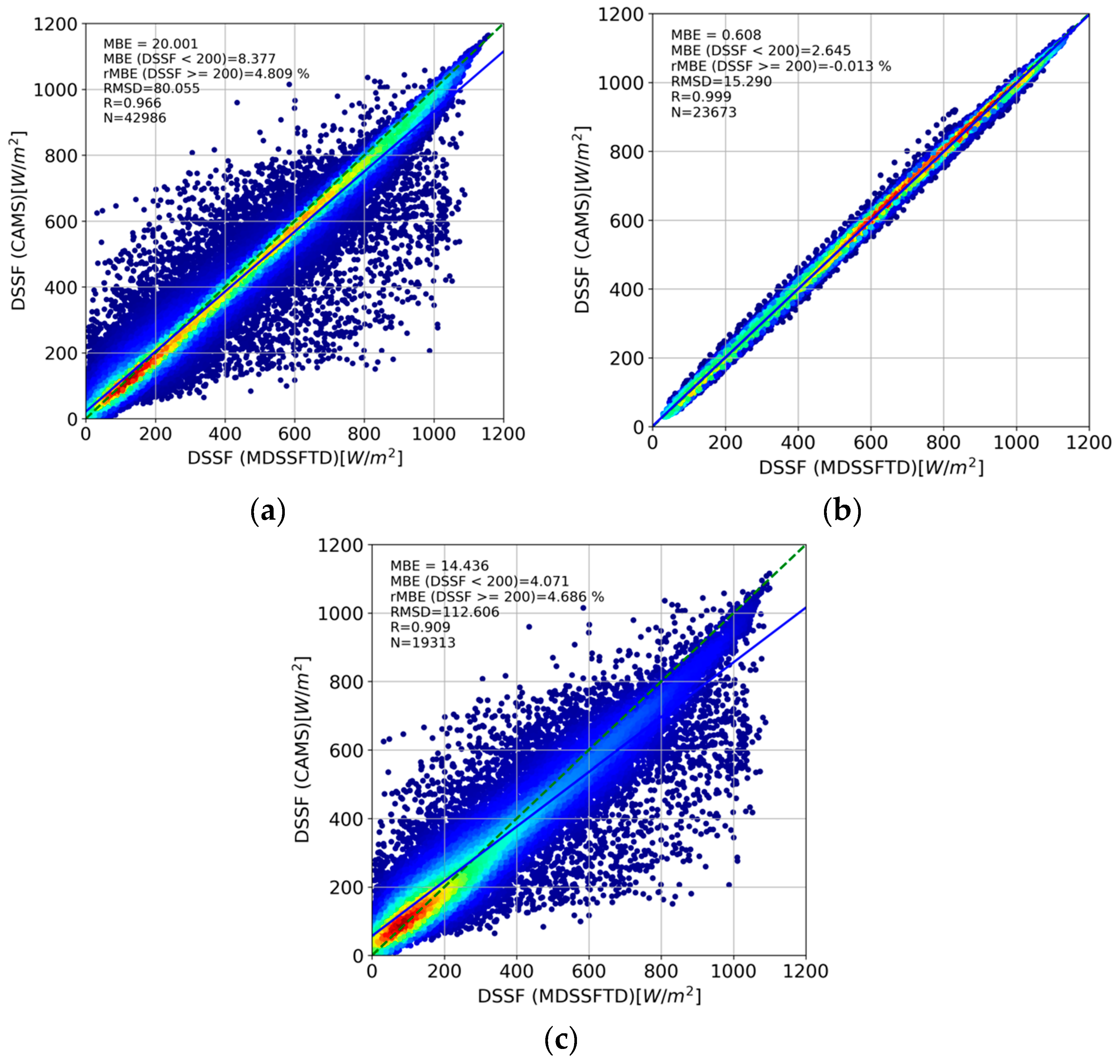
3.6. Comparison to the CAMS Radiation Product

The retrievals from MDSSFTD were compared against the counterpart estimates from the CAMS radiation product. Figure 18a shows the good agreement between the two products for all sky conditions, with a correlation of 0.966. Figure 18b,c take a further look at the comparison by exploring the clear sky and cloudy sky retrievals separately. The clear sky comparison indicates high agreement between the two products, which use the CAMS aerosol data as input. The comparison for cloudy sky conditions also shows good agreement (correlation of 0.909) despite the differences in the retrieval methods for cloudy sky conditions. The higher dispersion is justified by the increased difficulty of the retrieval for cloudy skies.

4. Conclusions

This paper presents the results of the comparison of the LSA-207 MDSSFTD product outputs, namely the total DSSF and diffuse fraction (fd) components, against in situ measurements acquired at four BSRN stations over a seven-month period. The validation was performed on instantaneous satellite retrievals with MSG/SEVIRI (i.e., acquired every 15 min).

The results showed that the satellite estimates of DSSF and fd meet the requirements for all sky (clear and cloudy) conditions. For DSSF, the requirements are 20 Wm⁻² for DSSF < 200 Wm⁻² and 10% for DSSF ≥ 200 Wm⁻². The MBE and rMBE compared to the ground measurements were found to be 3.618 Wm⁻² and 0.252%, respectively. For fd, the requirements are 0.1 for fd < 0.5 and 20% for fd ≥ 0.5. The MBE and rMBE compared to the ground measurements were −0.044% and −17.699%, respectively.

A more detailed analysis of the product performances was also performed separately for clear and cloudy sky conditions. For DSSF in clear sky conditions, the MBE and rMBE compared to the ground measurements were 8.637 Wm⁻² and 0.776%, respectively. For fd, the MBE and rMBE compared to the ground measurements were 0.062% and −22.197%, respectively. Thus, the two products’ outputs also met the target requirements if only clear sky conditions were selected and if the fd ≥ 0.5 case was not considered (which is not statistically representative). For DSSF in cloudy sky conditions, the MBE and rMBE compared to the ground measurements were −6.618 Wm⁻² and 2.782%, respectively. For fd, the MBE and rMBE compared to the ground measurements were 0.027% and −15.796%, respectively. Thus, the product met the target requirements for all conditions, with only a few exceptions. The major limitations of the retrieval approach described in the companion article [40] are not an obstacle in meeting the required quality. It is noted that the requirements for the product MDSSFTD were defined for the all sky conditions only.

In an earlier study by [42], it was shown that the use of MACC-II (now CAMS) AOD forecasts as input to the MDSSFTD clear sky method instead of re-analyses significantly decreased the quality of the DSSF products under clear sky conditions. For the last years, the quality of the CAMS AOD forecasts currently available could have improved, which means the high sensitivity of the MDSSFTD diffuse estimation to the quality of AOD forecasts is not a limitation anymore. Finally, we showed that this AOD information is of primary importance for the estimation of the atmospheric transmittance either in clear or cloudy conditions. In cloudy sky conditions, the modelling of the cloud–aerosol radiative coupling allowed a reduction of the overall bias by around 8%.

References

1. Mateos, D.; Antón, M.; Valenzuela, A.; Cazorla, A.; Olmo, F.J.; Alados-Arboledas, L. Short-wave radiative forcing at the surface for cloudy systems at a midlatitude site. Tellus B Chem. Phys. Meteorol. 2013, 65, 21069. [Google Scholar] [CrossRef]
2. Van Tricht, K.; Lhermitte, S.; Lenaerts, J.T.M.; Gorodetskaya, I.V.; L′Ecuyer, T.S.; Noël, B.; van den Broeke, M.R.; Turner, D.D.; van Lipzig, N.P.M. Clouds enhance Greenland ice sheet meltwater runoff. Nat. Commun. 2016, 7, 10266. [Google Scholar] [CrossRef] [PubMed]
3. Mercado, L.M.; Bellouin, N.; Sitch, S.; Boucher, O.; Huntingford, C.; Wild, M.; Cox, P.M. Impact of changes in diffuse radiation on the global land carbon sink. Nature 2009, 458, 1014. [Google Scholar] [CrossRef] [PubMed]
4. Carrer, D.; Roujean, J.L.; Lafont, S.; Calvet, J.C.; Boone, A.; Decharme, B.; Gastellu-Etchegorry, J.P. A canopy radiative transfer scheme with explicit FAPAR for the interactive vegetation model ISBA-A-gs: Impact on carbon fluxes. J. Geophys. Res. Biogeosci. 2013, 118, 888–903. [Google Scholar] [CrossRef]
5. O’Sullivan, M.; Rap, A.; Reddington, C.L.; Spracklen, D.V.; Gloor, M.; Buermann, W. Small global effect on terrestrial net primary production due to increased fossil fuel aerosol emissions from East Asia since the turn of the century. Geophys. Res. Lett. 2016, 43, 8060–8067. [Google Scholar] [CrossRef] [PubMed]
6. Yoshida, S.; Ueno, S.; Kataoka, N.; Takakura, H.; Minemoto, T. Estimation of global tilted irradiance and output energy using meteorological data and performance of photovoltaic modules. Sol. Energy 2013, 93, 90–99. [Google Scholar] [CrossRef]
7. Betts, A.K.; Hong, S.-Y.; Pan, H.-L. Comparison of NCEP–NCAR reanalysis with 1987 FIFE data. Mon. Weather Rev. 1996, 124, 1480–1498. [Google Scholar] [CrossRef]
8. Brotzge, J.A. A two-year comparison of the surface water and energy budgets between two OASIS sites and NCEP–NCAR reanalysis data. J. Hydrometeorol. 2004, 5, 311–326. [Google Scholar] [CrossRef]
9. Berbery, E.H.; Mitchell, K.E.; Benjamin, S.; Smirnova, T.; Ritchie, H.; Hogue, R.; Radeva, E. Assessment of land-surface energy budgets from regional and global models. J. Geophys. Res. 1999, 104, 19329–19348. [Google Scholar] [CrossRef]
10. Schroeder, T.A.; Hamber, R.; Copps, N.C.; Liang, S. Validation of solar radiation surfaces from MODIS and reanalysis data over topogra phically complex terrain. J. Appl. Meteorol. Clim. 2009, 48, 2441–2458. [Google Scholar] [CrossRef]
11. Babst, F.; Mueller, R.W.; Hollman, R. Verification ofNCEP reanalysis shortwave radiation with mesoscale remote sensing data. IEEE Trans. Geosci. Remote Sens. 2008, 5, 34–37. [Google Scholar] [CrossRef]
12. Urraca, R.; Huld, T.; Gracia-Amillo, A.; Martinez-de-Pison, F.J.; Kaspar, F.; Sanz-Garcia, A. Evaluation of global horizontal irradiance estimates from ERA5 and COSMO-REA6 reanalyses using ground and satellite-based data. Sol. Energy 2018, 164, 339–354. [Google Scholar] [CrossRef]
13. Bishop, J.K.B.; Rossow, W.B. Spatial and temporal variability of global surface solar irradiance. J. Geophys. Res. 1991, 96, 16389–16858. [Google Scholar] [CrossRef]
14. Darnell, W.; Staylor, W.; Gupta, S.; Denn, F. Estimation of surface insolation using sun-synchronous satellite data. J. Clim. 1988, 1, 820–835. [Google Scholar] [CrossRef]
15. Dedieu, G.P.; Deschamps, P.; Kerr, Y. Satellite estimation of solar irradiance at the surface of the earth and of surface albedo using a physical model applied to METEOSAT data. J. Clim. Appl. Meteorol. 1987, 26, 79–87. [Google Scholar] [CrossRef]
16. Gautier, C.; Diak, G.; Masse, S. A simple physical model to estimate incident solar radiation at the surface from GOES satellite data. J. Clim. Appl. Meteorol 1980, 19, 1005–1012. [Google Scholar] [CrossRef]
17. Cano, D.; Monget, J.M.; Albuisson, M.; Guillard, H.; Regas, N.; Wald, L. A method for the determination of the global solar radiation from meteorological satellite data. Sol. Energy 1986, 37, 31–39. [Google Scholar] [CrossRef]
18. Gautier, C.; Landsfeld, M. Surface solar radiation flux and cloud radiative forcing for the Atmospheric Radiation Measurement (ARM) Southern Great Plains (SGP): A satellite, surface observations, and radiative transfer model study. J. Atmos. Sci. 1997, 54, 1289–1307. [Google Scholar] [CrossRef]
19. Li, Z.; Leighton, H.G. Global climatologies of the solar radiation budgets at the surface and in the atmosphere from 5 years of ERBE data. J. Geophys. Res. 1993, 98, 4919–4930. [Google Scholar] [CrossRef]
20. Masuda, K.; Leighton, H.G.; Li, Z. A new parameterization for the determination of solar flux absorbed at the surface from satellite measurements. J. Clim. 1995, 8, 1615–1629. [Google Scholar] [CrossRef]
21. Hammer, A.; Heinemann, D.; Lorenz, E.; Lückehe, B. Short-term forecasting of solar radiation based on image analysis of meteosat data. In Proceedings of the EUMETSAT Meteorological Satellite Data Users Conference, Copenhagen, Denmark, 1999; pp. 331–337. [Google Scholar]
22. Möser, W.; Raschke, E. Incident solar radiation over Europe from METEOSAT data. J. Clim. Appl. Meteorol. 1984, 23, 166–170. [Google Scholar] [CrossRef]
23. Pinker, R.; Ewing, J. Modeling surface solar radiation: Model formulation and validation. J. Clim. Appl. Meteorol. 1985, 24, 389–401. [Google Scholar] [CrossRef]
24. Pinker, R.; Laszlo, I. Modeling surface solar irradiance for satellite applications on a global scale. J. Appl. Meteorol. 1992, 31, 194–211. [Google Scholar] [CrossRef]
25. Tarpley, J. Estimating incident solar radiation at the surface from geostationary satellite data. J. Clim. Appl. Meteorol. 1979, 18, 1172–1181. [Google Scholar] [CrossRef]
26. Whitlock, C.H.; Charlock, T.P.; Staylor, W.F.; Pinker, R.T.; Laszlo, I.; Ohmura, A.; Gilgen, H.; Konzelman, T.; DiPasquale, R.C.; Moats, C.D.; et al. First global WCRP shortwave surface radiation budget dataset. Bull. Am. Meteorol. Soc. 1995, 76, 905–922. [Google Scholar] [CrossRef]
27. Romano, F.; Cimini, D.; Cersosimo, A.; Di Paola, F.; Gallucci, D.; Gentile, S.; Geraldi, E.; Larosa, S.; Nilo, S.T.; Ricciardelli, E.; et al. Improvement in Surface Solar Irradiance Estimation Using HRV/MSG Data. Remote Sens. 2018, 10, 1288. [Google Scholar] [CrossRef]
28. Gallucci, D.; Romano, F.; Cersosimo, A.; Cimini, D.; Di Paola, F.; Gentile, S.; Geraldi, E.; Larosa, S.; Nilo, S.T.; Ricciardelli, E.; et al. Nowcasting Surface Solar Irradiance with AMESIS via Motion Vector Fields of MSG-SEVIRI Data. Remote Sens. 2018, 10, 845. [Google Scholar] [CrossRef]
29. Ineichen, P. High Turbidity Solis Clear Sky Model: Development and Validation. Remote Sens. 2018, 10, 435. [Google Scholar] [CrossRef]
30. Trigo, I.F.; DaCamara, C.C.P.; Viterbo, J.-L.; Roujean, F.; Olesen, C.; Barroso, F.; Camacho-de-Coca, D.; Carrer, S.C.; Freitas, J.; García-Haro, B.; et al. The Satellite Application Facility on Land Surface Analysis. Int. J. Remote Sens. 2011, 32, 2725–2744. [Google Scholar] [CrossRef]
31. Ineichen, P.; Barroso, C.S.; Geiger, B.; Hollmann, R.; Marsouin, A.; Mueller, R. Satellite Application Facilities irradiance products: Hourly time step comparison and validation over Europe. Int. J. Remote Sens. 2009, 30. [Google Scholar] [CrossRef]
32. Roerink, G.J.; Bojanowski, J.; de Wit, A.J.W.; Eerens, H.; Supit, I.; Leo, O.; Boogaard, H.L. Evaluation of MSG-derived global radiation estimates for application in a regional crop model. Agric. For. Meteorol. 2012, 160, 36–47. [Google Scholar] [CrossRef]
33. Moreno, A.; Gilabert, M.A.; Camacho, F.; Martínez, B. Validation of daily global solar irradiation images from MSG over Spain. Renew. Energy 2013, 60, 332–342. [Google Scholar] [CrossRef]
34. Bevan, S.L.; North, P.R.J.; Los, S.O.; Grey, W.M.F. A global dataset of atmospheric aerosol optical depth and surface reflectance from AATSR. Remote Sens. Environ. 2012, 116, 199–210. [Google Scholar] [CrossRef]
35. Jayaraman, A.; Lubin, D.; Ramachandran, S.; Ramanathan, V.; Woodbridge, E.; Collins, W.D.; Zalpuri, K.S. Direct observations of aerosol radiative forcing over the tropical Indian Ocean during the January-February 1996 pre-INDOEX cruise. J. Geophys. Res. Atmos. 1998, 103, 13827–13836. [Google Scholar] [CrossRef]
36. Satheesh, S.K.; Ramanathan, V. Large differences in tropical aerosol forcing at the top of the atmosphere and Earth′s surface. Nature 2000, 405, 60–63. [Google Scholar] [CrossRef] [PubMed]
37. Cherian, R.; Quaas, J.; Salzmann, M.; Wild, M. Pollution trends over Europe constrain global aerosol forcing as simulated by climate models. Geophys. Res. Lett. 2014, 41, 2176–2181. [Google Scholar] [CrossRef] [Green Version]
38. Dramé, M.S.; Ceamanos, X.; Roujean, J.L.; Boone, A.; Lafore, J.P.; Carrer, D.; Geoffroy, O. On the Importance of Aerosol Composition for Estimating Incoming Solar Radiation: Focus on the Western African Stations of Dakar and Niamey during the Dry Season. Atmosphere 2015, 6, 1608–1632. [Google Scholar] [CrossRef] [Green Version]
39. Kosmopoulos, P.G.; Kazadzis, S.; Taylor, M.; Athanasopoulou, E.; Speyer, O.; Raptis, P.I.; Marinou, E.; Proestakis, E.; Solomos, S.; Gerasopoulos, E.; et al. Dust impact on surface solar irradiance assessed with model simulations, satellite observations and ground-based measurements. Atmos. Meas. Tech. 2017, 10, 2435–2453. [Google Scholar] [CrossRef] [Green Version]
40. Carrer, D.; Ceamanos, X.; Moparthy, M.; Vincent, C.; Coehlo, S.; Trigo, I. Satellite retreival of downwelling shortwave surface flux and diffuse fraction under all sky conditions in the framework of the LSA SAF program (part 1: Methodology). Remote Sens. 2019, 11, 2532. [Google Scholar] [CrossRef] [Green Version]
41. Ceamanos, X.; Carrer, D.; Roujean, J.-L. An efficient approach to estimate the transmittance and reflectance of a mixture of aerosol components. Atmos. Res. 2014, 137, 125–135. [Google Scholar] [CrossRef]
42. Ceamanos, X.; Carrer, D.; Roujean, J.-L. Improved retrieval of direct and diffuse downwelling surface shortwave flux in cloudless atmosphere using dynamic estimates of aerosol content and type: Application to the LSA-SAF project. Atmos. Chem. Phys. 2014, 14, 8209–8232. [Google Scholar] [CrossRef] [Green Version]
43. Riihelä, A.; Kallio, V.; Devraj, S.; Sharma, A.; Lindfors, A. Validation of the Sarah-e satellite-based surface solar radiation estimates over India. Remote Sens. 2018, 10, 392. [Google Scholar] [CrossRef] [Green Version]
44. Riihelä, A.; Carlund, T.; Trentmann, J.; Müller, R.; Lindfors, A.V. Validation of CM SAF Surface Solar Radiation Datasets over Finland and Sweden. Remote Sens. 2015, 7, 6663–6682. [Google Scholar] [CrossRef] [Green Version]
45. Geiger, B.; Meurey, C.; Lajas, D.; Franchistéguy, L.; Carrer, D.; Roujean, J.L. Near real-time provision of downwelling shortwave radiation estimates derived from satellite observations. Meteorol. Appl. 2008, 15, 411–420. [Google Scholar] [CrossRef]
46. Carrer, D.; Lafont, S.; Roujean, J.-L.; Calvet, J.-C.; Meurey, C.; Le Moigne, P.; Trigo, I. Incoming solar and infrared radiation derived from METEOSAT: Impact on the modelled land waterand energy budget over France. J. Hydrometeorol. 2012, 13, 504–520. [Google Scholar] [CrossRef]
47. McArthur, L.J.B. Baseline Surface Radiation Network (BSRN)-Operation Manual Version 2.1; WMO/TD-No. 1274; WCRP/WMO, 2005; Available online: https://epic.awi.de/id/eprint/45991/1/McArthur.pdf (accessed on 8 November 2019).
48. Vuilleumier, L.; Hauser, M.; Félix, C.; Vignola, F.; Blanc, P.; Kazantzidis, A.; Calpini, B. Accuracy of ground surface broadband shortwave radiation monitoring. J. Geophys. Res. Atmos. 2014, 119, 13,838–13,860. [Google Scholar] [CrossRef] [Green Version]
49. García, R.D.; Cuevas, E.; Ramos, R.; Cachorro, V.E.; Redondas, A.; Moreno-Ruiz, J.A. Description of the Baseline Surface Radiation Network (BSRN) station at the Izaña Observatory (2009–2017): Measurements and quality control/assurance procedures. Geosci. Instrum. Methods Data Syst. 2019, 8, 77–96. [Google Scholar] [CrossRef] [Green Version]
50. Qu, Z.; Oumbe, A.; Blanc, P.; Espinar, B.; Gesell, G.; Gschwind, B.; Wald, L. Fast radiative transfer parameterisation for assessing the surface solar irradiance: The Heliosat-4 method. Meteorol. Z. 2017, 26, 33–57. [Google Scholar] [CrossRef]
51. Lefèvre, M.; Oumbe, A.; Blanc, P.; Espinar, B.; Gschwind, B.; Qu, Z.; Benedetti, A. McClear: A new model estimating downwelling solar radiation at ground level in clear-sky conditions. Atmos. Meas. Tech. 2013, 6, 2403–2418. [Google Scholar] [CrossRef] [Green Version]
52. Gschwind, B.; Wald, L.; Blanc, P.; Lefèvre, M.; Schroedter-Homscheidt, M.; Arola, A. Improving the McClear model estimating the downwelling solar radiation at ground level in cloud-free conditions–McClear-v3. Meteorol. Z. 2019, 28, 147–163. [Google Scholar] [CrossRef]
53. Mayer, B.; Kylling, A. The libRadtran software package for radiative transfer calculations-description and examples of use. Atmos. Chem. Phys. 2005, 5, 1855–1877. [Google Scholar] [CrossRef] [Green Version]
54. Blanc, P.; Gschwind, B.; Lefèvre, M.; Wald, L. Twelve monthly maps of ground albedo parameters derived from MODIS data sets. In Proceedings of the IGARSS 2014, Quebec City, QC, Canada, 3–18 July 2014; pp. 3270–3272. [Google Scholar]
55. Schaaf, C.B.; Gao, F.; Strahler, A.H.; Lucht, W.; Li, X.; Tsang, T.; Lewis, P. First operational BRDF, albedo nadir reflectance products from MODIS. Remote Sens. Environ. 2002, 83, 135–148. [Google Scholar] [CrossRef] [Green Version]
56. Kriebel, K.T.; Saunders, R.W.; Gesell, G. Optical properties of clouds derived from fully cloudy AVHRR pixels. Beiträge zur Physik der Atmosphäre 1989, 62, 165–171. [Google Scholar]
57. Kriebel, K.T.; Gesell, G.; Ka Stner, M.; Mannstein, H. The cloud analysis tool APOLLO: Improvements and validations. Int. J. Remote Sens. 2003, 24, 2389–2408. [Google Scholar] [CrossRef]
58. Hakuba, M.Z.; Folini, D.; Sanchez-Lorenzo, A.; Wild, M. Spatial representativeness of ground-based solar radiation measurements. J. Geophys. Res. 2013, 118, 8585–8597. [Google Scholar] [CrossRef] [Green Version]
59. Erbs, D.G.; Klein, S.A.; Duffie, J.A. Estimation of the diffuse radiation fraction for hourly, daily and monthly-average global radiation. Sol. Energy 1982, 28, 293–302. [Google Scholar] [CrossRef]
60. Reindl, D.T.; Beckman, W.A.; Duffie, J.A. Diffuse fraction correlations. Sol. Energy 1990, 45, 1–7. [Google Scholar] [CrossRef]
61. Orgill, J.F.; Hollands, K.G.T. Correlation equation for hourly diffuse radiation on a horizontal surface. Sol. Energy 1977, 19, 357–359. [Google Scholar] [CrossRef]
62. Louche, A.; Notton, G.; Poggi, P.; Simonnot, G. Correlations for direct normal and global horizontal irradiation on French Mediterranean site. Sol. Energy 1991, 46, 261–266. [Google Scholar] [CrossRef]
Figure 1. Location of the ground stations providing in situ measurements.
Remotesensing 11 02630 g001
Figure 2. Diffuse fraction components retrieved following four empirical formulations, (a) Erbs et al. [59], (b) Orgill and Hollands [61], (c) Louche et al. [62], and (d) Reindl et al. [60] compared to the in situ diffuse fraction component. The blue color corresponds to a low density of points and the red color corresponds to a high density of points. The blue line represents the mean fit across all evaluation data; the green line is the 1:1 line.
Remotesensing 11 02630 g002
Figure 3. Diurnal variation of the total MDSSFTD component in clear sky conditions compared against in situ measurements for (a) Carpentras, (b) De Aar, (c) Tamanrasset, and (d) Toravere for a selected day. Yellow cloudy samples do not appear in this figure as the chosen dates were fully clear.
Remotesensing 11 02630 g003
Figure 4. Diurnal variation of the diffuse fraction MDSSFTD component in clear sky conditions compared against in situ measurements for (a) Carpentras, (b) De Aar, (c) Tamanrasset, and (d) Toravere for a selected day. Yellow cloudy samples do not appear in this figure as the chosen dates were fully clear.
Remotesensing 11 02630 g004
Figure 5. Diurnal variation of the total MDSSFTD component in all sky conditions compared against in situ measurements for (a) Carpentras, (b) De Aar, (c) Tamanrasset, and (d) Toravere for a selected day (partially clear and cloudy). The yellow dots represent cloudy retrievals and the blue dots represent clear sky retrievals.
Remotesensing 11 02630 g005
Figure 6. Diurnal variation of the diffuse fraction of MDSSFTD in all sky conditions compared against in situ measurements for (a) Carpentras, (b) De Aar, (c) Tamanrasset, and (d) Toravere for a selected day (partially clear and cloudy). The yellow dots represent cloudy retrievals and the blue dots represent clear sky retrievals.
Remotesensing 11 02630 g006
Figure 7. Comparison of instantaneous MSG-derived MDSSFTD measurements for (a) total DSSF, (b) diffuse fraction components with their in situ counterparts for clear sky retrievals. The retrievals were collected every 15 min. The blue line represents the mean fit across all evaluation data; the green dashed line to the 1:1 line. The blue circles correspond to a low density of points and the red circles correspond to a high density of points.
Remotesensing 11 02630 g007
Figure 8. Comparison of instantaneous MSG-derived MDSSFTD measurements for (a) total and (b) diffuse fraction components with their in situ counterparts for cloudy sky retrievals. The retrievals were collected every 15 min. The blue line represents the mean fit across all evaluation data; the green dashed line is the 1:1 line. The blue circles correspond to a low density of points and red circles correspond to a high density of points.
Remotesensing 11 02630 g008
Figure 9. Comparison of instantaneous MSG-derived MDSSFTD measurements for (a) total and (b) diffuse fraction components with their in situ counterparts for all sky (clear and cloudy) retrievals. The retrievals were collected every 15 min. The blue line represents the mean fit all evaluation data; the green dashed line to the 1:1 line. The blue circles correspond to a low density of points and the red circles correspond to a high density of points.
Remotesensing 11 02630 g009
Figure 10. Time series of the statistics of differences averaged on a daily basis between 15-min in situ measurements and 15-min MDSSFTD total flux (blue dots). The daily standard deviations of the absolute and relative statistics are indicated with vertical blue lines. The data points were filtered to keep those (a) total flux values less than 200 Wm−2 (absolute statistics) and (b) total flux values greater than 200 Wm−2 (relative statistics). The comparison was made only for the clear sky conditions. The green dotted horizontal lines characterize the “target” accuracy requirements; the red dotted line is the reference line (no error).
Remotesensing 11 02630 g010
Figure 11. Same as Figure 10 but for cloudy sky conditions.
Remotesensing 11 02630 g011
Figure 12. Same as Figure 10 but for all sky (clear and cloudy) conditions.
Remotesensing 11 02630 g012
Figure 13. Time series of the relative mean bias for the comparison of the diffuse fraction on the 15-min time step basis. The statistics of differences were averaged on a daily basis. The standard deviations of the relative statistics are indicated with vertical blue lines. The data points were filtered to keep those (a) diffuse fraction values less than 0.5 (absolute statistics) and (b) diffuse fraction values greater than or equal to 0.5 (relative statistics). The comparison was made only for clear sky conditions. The green dotted horizontal lines characterize the “target’ requirements; the red dotted line is the reference line (no error).
Remotesensing 11 02630 g013
Figure 14. Same as Figure 13 but for cloudy sky conditions.
Remotesensing 11 02630 g014
Figure 15. Same as Figure 13 but for all sky (clear and cloudy) conditions.
Remotesensing 11 02630 g015
Figure 16. Same diurnal variation as in Figure 5 for Carpentras. Light-blue dots show the estimations of total MDSSFTD with ‘no coupling’ (i.e., no activation of the cloud–aerosol coupling) in cloudy conditions. Yellow dots show the same LSA-207 DSSF retrievals in cloudy conditions as those in Figure 5. The black dashed line represents the AOD (CAMS). The statistics in the top right corner are those of the MDSSFTD product (with activation of the cloud–aerosol coupling).
Remotesensing 11 02630 g016
Figure 17. Same as Figure 11 for cloudy sky conditions but with inactivation of the coupling between the cloud and aerosol.
Remotesensing 11 02630 g017
Figure 18. Density scatter plots for the comparison between the MDSSFTD and CAMS radiation product for (a) all sky, (b) clear sky, and (c) cloudy sky conditions. The blue line represents the mean fit all evaluation data; the green dashed line is the 1:1 line.
Remotesensing 11 02630 g018