Going Deeper with Densely Connected Convolutional Neural Networks for Multispectral Pansharpening

1
School of Computer Science, National Engineering Laboratory for Integrated Aero-Space-Ground-Ocean Big Data Application Technology, Shaanxi Provincial Key Laboratory of Speech & Image Information Processing, Northwestern Polytechnical University, Xi’an 710129, China
2
Shaanxi Key Laboratory of Intelligent Processing for Big Energy Data, School of Physics and Electronic Information, Yan’an University, Yan’an 716000, China
3
Department of Electronics and Informatics, Vrije Universiteit Brussel, 1050 Brussels, Belgium
*
Author to whom correspondence should be addressed.
Remote Sens. 2019, 11(22), 2608; https://doi.org/10.3390/rs11222608
Submission received: 13 October 2019
/
Revised: 30 October 2019
/
Accepted: 4 November 2019
/
Published: 7 November 2019
(This article belongs to the Section Remote Sensing Image Processing)
Abstract
:In recent years, convolutional neural networks (CNNs) have shown promising performance in the field of multispectral (MS) and panchromatic (PAN) image fusion (MS pansharpening). However, the small-scale data and the gradient vanishing problem have been preventing the existing CNN-based fusion approaches from leveraging deeper networks that potentially have better representation ability to characterize the complex nonlinear mapping relationship between the input (source) and the targeting (fused) images. In this paper, we introduce a very deep network with dense blocks and residual learning to tackle these problems. The proposed network takes advantage of dense connections in dense blocks that have connections for arbitrarily two convolution layers to facilitate gradient flow and implicit deep supervision during training. In addition, reusing feature maps can reduce the number of parameters, which is helpful for reducing overfitting that resulted from small-scale data. Residual learning is explored to reduce the difficulty for the model to generate the MS image with high spatial resolution. The proposed network is evaluated via experiments on three datasets, achieving competitive or superior performance, e.g. the spectral angle mapper (SAM) is decreased over 10% on GaoFen-2, when compared with other state-of-the-art methods.
1. Introduction
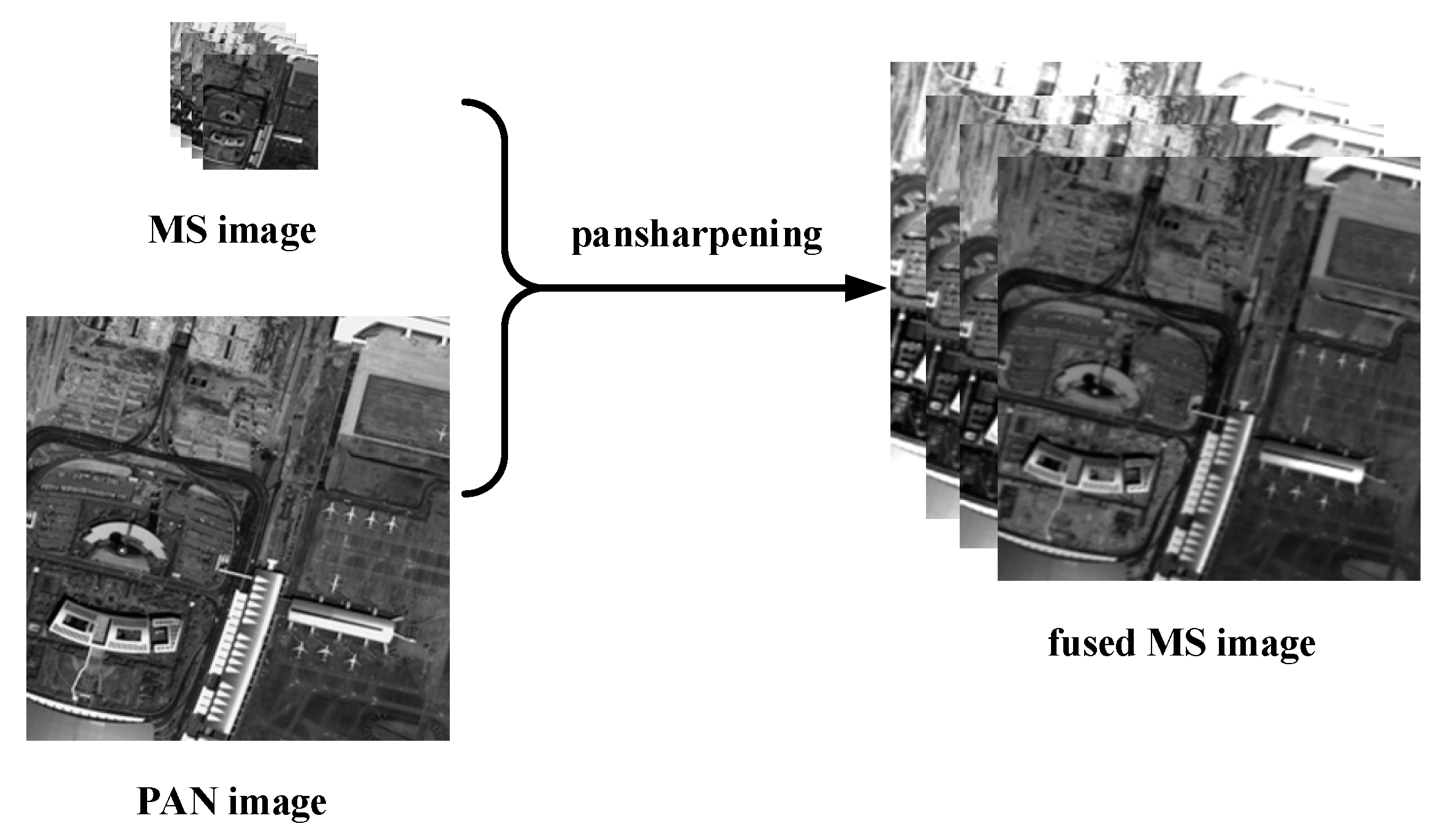
Remote sensing images are widely used in many fields, e.g., agriculture, forestry, geology, meteorology, environmental protection, etc. [1]. Especially in recent years, commercial products (such as Google Earth and Bing Maps) using remote sensing images is increasing, which has boosted the demand for remote sensing images. These images have two important properties—spectral resolution and spatial resolution. Spectral resolution refers to the number of spectral bands or the minimum spectral bandwidth, while spatial resolution is about the dimension or size of the smallest unit that can be distinguished. Ideally, remote sensing applications require images with high spatial and spectral resolution. However, due to the compromise between data storage and signal-to-noise ratio, such ideal images are difficult to be obtained by a single sensor. Therefore, many satellites (such as IKONOS, GaoFen-2, and WorldView-2) carry two optical sensors to simultaneously capture two types of images that have different but complementary properties of the same geographical area. One of the sensors captures panchromatic (PAN) single-band images with high spatial resolution, while the other collects multispectral (MS) images at lower spatial resolution. While PAN images have higher spatial resolution than MS images, the former has less spectral information. In practical applications, the spectral information and the sharpness of targets in remote sensing images are crucial for interpretation and analysis. Therefore, MS images with a high spatial resolution are often required on many and various occasions. MS pansharpening [2,3] is to use detail information in PAN images to enhance the spatial resolution of MS images (Figure 1). MS pansharpening has been an important pre-processing step in various remote sensing tasks e.g. change detection [4], target recognition [5], image classification [6], etc.
In the past few decades, various methods have been proposed for MS pansharpening. Traditional pansharpening methods [7] include component substitution (CS) [8,9,10], multi-resolution analysis (MRA) [11,12], model-based optimization [13], and other methods [14,15,16]. Most of these methods can effectively fuse PAN and MS images in some respect, e.g., they can improve the spatial resolution of MS images and maintain their original spectral information to a certain extent. However, they have some limitations. For CS and MRA, there is a contradiction between retaining the spectral information in MS images and improving the spatial resolution of it, especially when the spectral range of MS images and that of PAN images are not the same [17]. Model-based optimization methods rely heavily on prior knowledge and hyper-parameters. Inappropriate selection of prior knowledge and hyper-parameters will reduce their performance.
More recently, our community has witnessed the significant success of deep learning technology in related research fields, e.g., classification, super-resolution, segmentation [18]. Researchers have applied this technology, especially, convolutional neural networks (CNNs), to pansharpening. Masi et al. [17] proposed the first CNN based pansharpening method (PNN), the structure of which is similar to super-resolution convolutional neural network (SRCNN) [19]. Their network has only three convolutional layers, which are not enough to map the complex mapping relationship in the field of pansharpening. Yuan et al. [20] designed a multi-scale and multi-depth CNN (MSDCNN), which has two branches with different number of learnable layers. However, even the deep branch has only five learnable layers. Inspired by PNN, Liu et al. [21] demonstrated the high flexibility of CNN design, and proposed a two-stream fusion network (TFNet), which divides the whole network into feature extraction, feature fusion, and reconstruction. They also built the ResTFNet with residual blocks and achieved state-of-arts results. Nevertheless, the structure of their network still needs to be further improved.
From the above, it should be pointed out that CNNs for MS pansharpening become deeper and deeper. In the computer vision community, the same trend can be found. In 2012, Alex et al. [22] trained a CNN (AlexNet) that contains only eight layers. Two years later, Simonyan et al. [23] introduced VGG-Net and thoroughly evaluated the network of increasing depth using an architecture with very small (3 × 3) convolution filters, which shows that a significant improvement on the prior-art configurations can be achieved by pushing the depth to 16–19 layers. In the same year, Szegedy et al. [24] proposed GoogLeNet, a 22-layer deep CNN, the quality of which is assessed in the context of classification and detection. It is reasonable because CNNs with a deeper architecture can map more complex nonlinearity relationship. However, a large number of layers results in gradient vanishing and exploding during training, requires large-scale data, and consumes much of computation. Many works focus on how to solve or abate these problems. In 2016, He et al. [25] first introduced the concept of residual learning and proposed residual neural networks (ResNets). The ResNets can gain accuracy from considerably increased depth (152 layers). Huang et al. [26] extend the concept of residual learning to extreme and construct densely connected convolutional networks (DenseNets) with dense connections. The proposed dense connections connect all layers in the same dense block. This kind of connections facilitates gradient flow, encourages feature reuse, and enhances implicit deep supervision whereas DenseNets require less computation and outperform most of state-of-the-art networks.
In order to reduce the effect of gradient vanishing or exploding problems and to reduce computation, we extend the concept of dense connection to pansharpening. In addition, residual learning is explored to reduce the difficulty of constructing the MS image with high spatial resolution. The contributions of this work are listed below:
1. We introduce a deeper CNN with dense blocks than other existing deep networks for pansharpening. The proposed network takes advantage of dense connections that have connections for arbitrarily two convolution layers in dense blocks to facilitate gradient flow and implicit deep supervision during training. With a deeper structure (44 learnable layers), the proposed network can learn the complex nonlinearity mapping relationship between the source and the target in the field of pansharpening.
2. Residual learning is explored to further boost the performance of the proposed network. With residual learning, the original spectral information can be fully injected into the fused image without any processing. In this way, the network just needs to learn how to construct residual instead of the high spatial resolution MS image, so that the difficulty for reconstruction can be reduced.
3. Both quantitative evaluation with established indexes and qualitative evaluation through visual inspection are adopted to compare the proposed network with various methods. Experimental results demonstrate that the proposed method can achieve state-of-the-art results.
This paper is organized as follows. Related works are discussed in Section 2. Section 3 is devoted to the description of the proposed very deep CNN. The description of experimental results, followed by some analysis of the obtained results, is introduced in Section 4. Finally, the paper is concluded in Section 5.
2. Related Work
2.1. Traditional Pansharpening Methods
Traditional methods have promoted the development of MS pansharpening. We briefly describe these methods below.
In CS methods, MS images are upsampled to the same spatial resolution as PAN images and then transformed into another feature space. They assume that spectral information and spatial information are separable. Therefore, the upsampled MS image can be projected into different components. The PAN images then totally or partially replace the spatial component of the MS images to enhance spatial resolution. If the correlation between the components is low and the correlation between the PAN image and the replaced component is high, the CS method can produce the high spatial resolution MS images with little distortion. Before the replacement, the PAN image and the replaced component need to be matched by their histograms, which is a crucial preprocessing step. The last step of CS methods is to project the fused images back into the original space by an inverse transformation.
MRA methods assume that the missed spatial detail information of MS images can be supplemented by the high-frequency spatial component in PAN images. The basic idea of MRA is to inject the high-frequency information of PAN images into MS images while maintaining all information of MS images. The most common MRA method is the High-Pass Filter (HPF) algorithm [27], which directly extracts high-frequency information of PAN images with a high-pass filter and then injects the high-frequency information into MS images.
Model-based optimization methods use sparse representation and compressed sensing to find an overcomplete dictionary of MS and PAN images [28]. The overcomplete dictionary can be obtained by solving the sparse coefficients through optimization techniques, and it is then used to reconstruct high resolution images [29]. In [30], an MS pansharpening method based on compressed sensing theory and sparse representation is proposed, where the sparseness in the expected high-resolution MS images is used to reconstruction the high spatial resolution MS images. The model proposed in [31] learns a dictionary from a mixed data set of PAN and upsampled MS images. This method does not require a large number of training images. Based on the scale invariance, Xiao et al. [32] assume that the low-resolution image and the corresponding high-resolution image have the same sparse coefficient under a pair of coupled dictionaries. So after solving the sparse coefficients of a low resolution image under the low resolution dictionary, the corresponding high resolution image can be reconstructed by multiplying the obtained sparse coefficients with the atoms of the coupled high resolution dictionary.
Other types of methods, hybrid methods, are mixtures of different methods [33]. As discussed in previous sections, CS and MRA methods have their obvious advantages and disadvantages. CS methods have better performance in improving the spatial quality of fused images, but they are prone to spectral distortion. The MRA methods can better preserve the spectral information of original MS images but often cause spatial distortion. These issues naturally lead to the idea of combining CS and MRA to form hybrid methods that take advantages of both so that spectral and spatial distortion problems can be addressed.
2.2. CNN Based Pansharpening Methods
Masi et al. [17] proposed the first CNN based pansharpening method (PNN). They discussed the intrinsic relationship between super-resolution and MS pansharpening. The proposed PNN is similar to the SRCNN [19], but they have something different, e.g., SRCNN has just one input, while PNN stacks the PAN and up-sampled MS images to form a five-band input. In addition, PNN introduces prior knowledge of specific remote sensing image data to the network to guide the training process. PNN achieved better results than traditional methods.
Recently, some MS pansharpening networks have adopted the idea of residual learning to further improve their performance. Due to the sample structure of PNN which has only a simple three learnable layers, some works also tried to use residual learning to boost the performance of PNN. To speed up the training of PNN and improve the performance, Scarpa et al. [34] added residual learning to PNN and obtained a significant performance gain over state-of-the-art methods.
Wei et al. [35] introduced the concept of residual learning and formed a deep CNN (11 learnable layers) to make full use of the high non-linearity of deep learning models. The proposed network directly connects the input image to the second last layer of the network by a skip connection. This practice can better preserve the information of original MS and PAN images, and reduces potential spectral and spatial distortions.
Later, to improve the spatial quality of the fused image, Yang et al. [36] designed an MS pansharpening model called PanNet. The main body of the network is 10 stacked residual blocks and it takes the highpass components of MS and PAN images as input. It transmits spectral information of MS images through residual learning. PanNet explicitly divides the two basic objectives of MS pansharpening, thus reducing the complexity of the problem. Moreover, using high-pass components of MS and PAN images instead of original images as input is advantageous for the network to generalize between image datasets from different satellites
Yuan et al. [20] proposed the MSDCNN consisting of a shallow branch and a deep branch. The shallow branch directly adopts PNN to extract simple features, while the deep branch uses two stacked blocks to extract image features of different scales. Even the deep branch has only five learnable layers in depth. In order to ensure that information can be more efficiently transmitted from front layers to back layers, skip connections are also added to Inception blocks. Eventually, the outputs of the shallow and deep branch are added together to generate high spatial resolution MS images.
More recently, Liu et al. [21] proposed the TFNet, which exhibits high flexibility of CNN design. Inspired by PNN, the whole network structure of TFNet can be divided into three sub-networks whose functions are feature extraction, feature fusion, and image reconstruction, respectively. The feature extraction sub-network consists of two branches to respectively extract spatial and spectral features from the input MS and PAN images. The obtained feature maps are then concatenated and put to the feature fusion sub-network. The features fused by concatenation, and three convolution layers are used to get a more compact feature. Afterward, the feature is transmitted to the image reconstruction sub-network which has eleven convolution layers and outputs the final fused image. Nevertheless, there is something needed to be improved, e.g., each convolutional layers are followed by a Batch Normalization (BN) layer which is abundant to achieve better results in many relevant tasks [37], there will be a large number of parameters and much of computation to increase the depth of their networks with the limit of data sets and computation resources.
3. The Proposed Network
The proposed network contains three modules. The first module extracts spatial and spectral features from PAN and MS images. The second module fuses the extracted features with dense blocks and the last module reconstructs high spatial resolution MS images with residual learning. In this section, we formulate the fusion problem and introduce the architecture of our model. Feature extraction, feature fusion, and reconstruction modules are then introduced.
3.1. Problem Formulation
The MS pansharpening problem can be divided into three sub-problems: how to extract features of PAN and MS images, how to fuse the features, and how to reconstruct high spatial resolution MS images. These sub-problems are solved by three modules: feature extraction, feature fusion, and reconstruction. For convenience, we use E(·) to denote the feature extraction module, where EM(·) and EP(·) can extract spectral and spatial features from MS and PAN images respectively. F(·) and R(·) denote the feature fusion and image reconstruction modules. The pansharpening model is formulated as follows:
where represents the PAN image and the corresponding MS image is denoted by , and are extracted features and they are then fused by F(·). The reconstruction module takes not only the fused feature but also the extracted features, which can facilitate the gradient flow. In order to reduce the difficulty of high spatial resolution MS image reconstruction, is put into the reconstruction module to realize residual learning.
3.2. Architecture
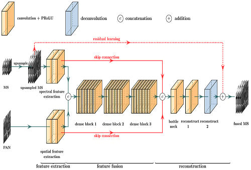
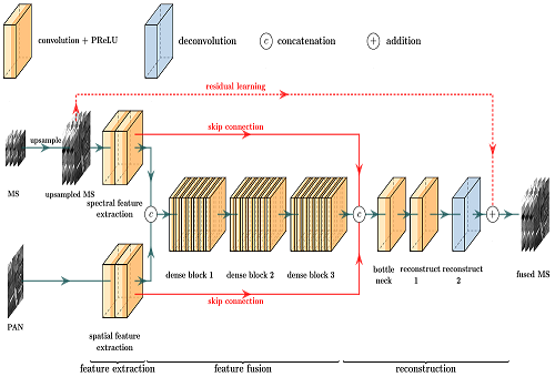
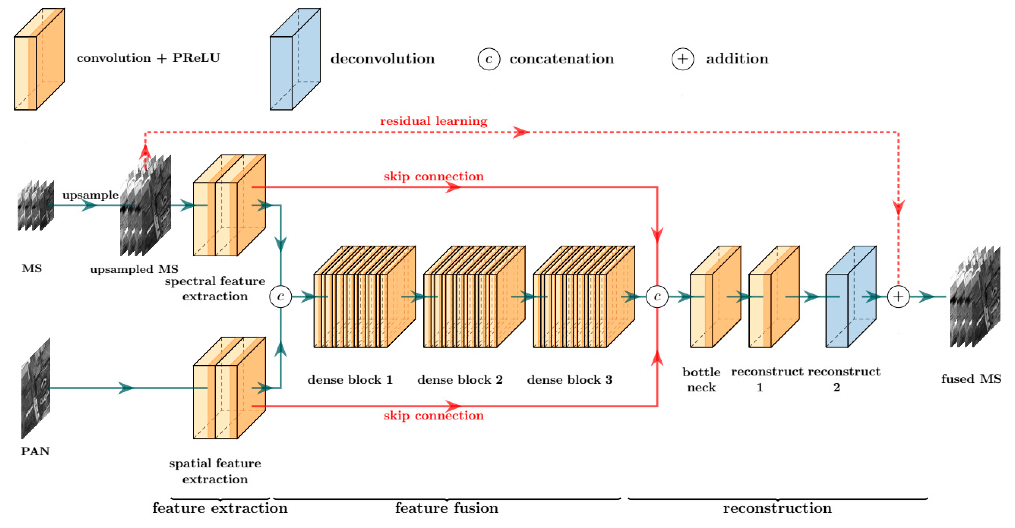
Inspired by the high-performance of deep CNNs in classification and other related tasks, a very deep fully convolutional network is designed for MS pansharpening. Figure 2 shows the detail of the proposed network. Legends are at the top of the figure: one convolutional layer, one de-convolutional layer, and two fusion operations. Each orange cuboid represents a convolutional layer, where the dark part denotes activation function PReLU and the light part is convolution operation. The blue cuboid is a de-convolutional layer that does not have the dark part, which means that the activation function does not exist in the de-convolutional layer. ![Remotesensing 11 02608 i001]() and
and ![Remotesensing 11 02608 i002]() are concatenation and addition fusion operations respectively.
are concatenation and addition fusion operations respectively.
 and
and  are concatenation and addition fusion operations respectively.
The proposed network is demonstrated below legends and it can be trained in an end-to-end manner. It can be seen that the network takes a PAN image and an upsampled MS image as inputs and has three modules, e.g., feature extraction, feature fusion, and reconstruction. Spatial and spectral features are extracted separately. The extracted features are stacked together and fused by three consecutive dense blocks in the feature fusion module. The fused feature is concatenated with the extracted features by skip connections and then pass through the bottleneck layer in the reconstruction module. The high spatial resolution MS image is reconstructed from these features at the end of the network. As three modules can be merged as one network, the proposed network is trained in an end-to-end manner.
The proposed network takes advantage of deep CNNs that they can simulate the nonlinear mapping relationship between input and target. The proposed network follows the architecture of VGG-net, where convolutional layers with small kernels are stacked e.g., spatial size of convolutional kernels is not larger than 3 × 3. Small kernels also help reduce the number of parameters and decrease training time. The depth of the proposed network reaches 44 convolutional layers which is much deeper than many state-of-the-art networks. In general, a deep network is superior to a shallow one because the deep network has a better nonlinearity, which can help the model to fit the complex mapping relationship between inputs and reference MS images and to learn more abstract and representative features.
3.3. Feature Extraction
Two sub-networks are used to extract spatial and spectral features separately. These sub-networks have the same architecture, but their parameters (e.g., weights and biases) are different. One of the sub-networks takes MS images as input, while PAN images are fed to the other. Two feature extraction sub-networks are composed of two consecutive convolutional layers whose convolutional kernels are all 3 × 3, and the extracted features are then put into the subsequent network. Many CNNs use maximum pooling or average pooling to obtain the scale invariance and rotation invariance of features. However, the texture and minutiae information is especially important in the topic of MS pansharpening. In order to avoid loss information during image processing, no down-sampling operation is used in the entire network. The formulations of the two sub-networks are:
where, ∗ is convolution operation, denotes kernel weight, b represents bias, and the activation function (parametric rectified linear unit) is denoted as PreLU(·).
3.4. Feature Fusion
The feature fusion module takes and as input and fused them together to produce a compact and concise feature. The fused feature F needs to combine the advantages of and . Although is considered as a carrier of spatial information, spectral information exists in it too. Similarly, it is verified that contains spectral information, but it cannot be denied that it also contains its spatial information (low frequency). Three dense blocks are used to fuse these features, which is demonstrated in Figure 2. Inspired by [37], the BN layers used in [38] are removed in the equipped dense blocks. and are concatenated and then fused by three dense blocks, which is formulated as:
where D(·) indicates a dense block, “ⓒ” represents the concatenation operation. Here, the concatenation operation explicitly combines the two feature maps and clearly reflects the concept of image fusion that integrating information from different image features. Another advantage of the concatenation operation is the relatively high efficiency. Subsequently, the concatenated feature is put into the dense blocks, and the dense blocks will output a fused feature that is more compact than the concatenated feature. The resulting fused feature can be regarded as a feature containing all spatial and spectral information of and .
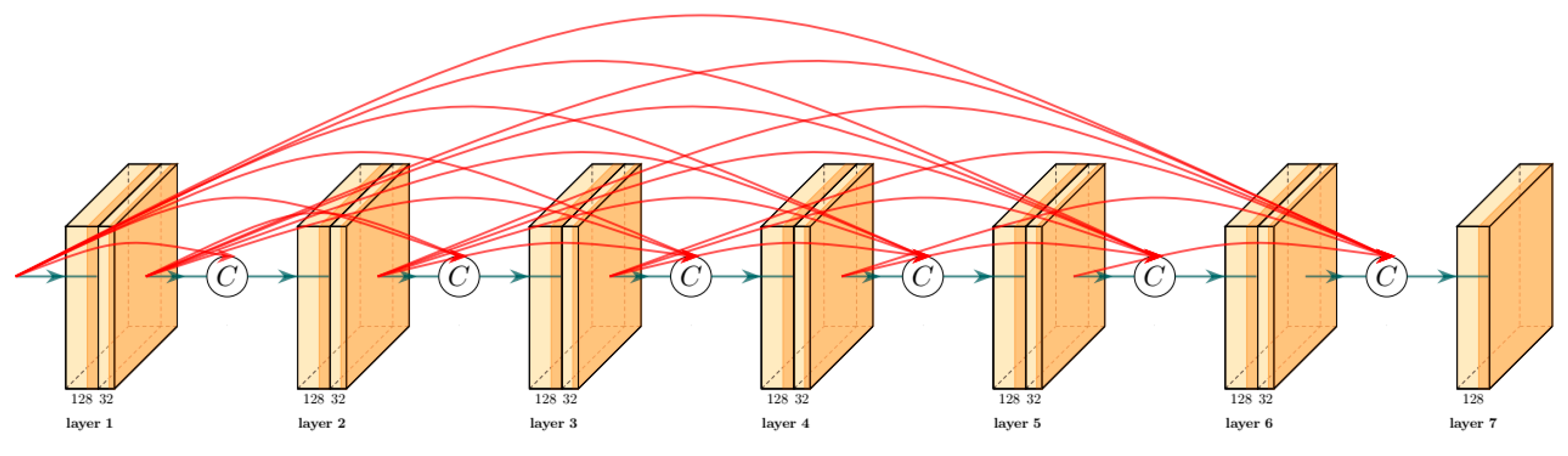
Dense blocks are easy to implement but effective. In traditional CNNs, if the network is stacked by L layers, there will be L + 1 connections between layers in the network. When it comes to dense blocks, there are L(L + 1)/2 connections. Figure 3 shows these connections, where arbitrary two layers are directly connected. In other words, the input of each layer of a dense block is the union of feature maps generated by previous layers, and the output feature map will be shared to all subsequent layers by connection. This structure can be defined as:
where [x0, x1, ⋯, xL−1] indicates that the feature maps from 0 to L − 1 layer are concatenated according to the feature dimension. The process [] is a concatenation operation rather than an addition operation like residual blocks. DL represents the transform function of the L-th layer, which includes two consecutive convolutional layers. The former convolutional layer is a bottleneck layer with a 1 × 1 kernel while the later has a 3 × 3 convolution kernel. The channel numbers of their output feature maps are 128 and 32. The bottleneck layer is indispensable because with more layers in dense blocks more feature maps need to be concatenated which results in a large number of channels of feature maps that consume much of GPU memory and computation. Therefore, the number of channels should be set to small, to reduce the redundancy and computational complexity of dense blocks. To further reduce the computational burden, the 1 × 1 convolutional bottleneck layer in front of each 3 × 3 convolutional layer is used to reduce the number of channels. It not only greatly reduces the amount of calculation, but also integrates each feature map without losing information. In order to realize the concatenation of the feature map, all feature maps have the same spatial size in a dense block, so the step sizes are set to one and no down-sampling operation is used.
xL = DL([x0, x1, ⋯, xL−1]),
3.5. Reconstruction
The final stage of the proposed network is to reconstruct the desired high spatial resolution MS image from the fused feature. Although it is at the rear of the network, the last is not the least. There are three different convolutional layers: a 1 × 1 convolutional layer, a 3 × 3 convolutional layer, and a de-convolutional layer. Residual learning and skip connections are adopted in this module. It can be formulated as follows:
where the ΦR denotes the stacked layers of reconstruction module, F is the output feature of the fusion module, and are the extracted features, and ⓒ is the concatenation operation. It can be seen from Equation (5) and Figure 2 that the fused and extracted features are concatenated and then reconstruct the residual between the MS and fused images.
There are three layers in the module. The first one is a bottleneck layer with a 1 × 1 kernel. The second is a convolutional layer with 3 × 3 kernel. It should be noted that the last one is a de-convolution layer that is also the last layer of the entire network. So its activation function PReLU is removed. De-convolution is a special kind of convolution. Its function in forward and backward propagations is just opposite to that of an ordinary convolution [39]. That is to say, the forward propagation process of an ordinary convolution layer is the backward propagation process of a de-convolution layer, and the backward propagation process of a convolution layer is the forward propagation of a deconvolution layer. Therefore, if convolution layers correspond to the image encoding process, then deconvolution layers correspond to the image decoding process.
Residual learning is also equipped in this module to reduce the difficulty of MS image reconstruction. In Figure 2, the red dash line indicates residual learning. This line connects the input and the fused MS images. The practical implementation is very simple but effective. It only needs to add the input MS image with the output of the last layer. The reconstruction module only needs to reconstruct the residual instead of the high spatial resolution MS image.
In the proposed network, gradient flow is also facilitated by skip connections between modules. The feature extraction module is too far away from the reconstruction module. It is reasonable for us to build information highways between the modules. By skip connections, the diversity of input features of the reconstruction module is increased, and the difficulty of network training can be alleviated. The constructed information highway can alleviate exploding gradient and vanishing gradient problems, thus accelerating the convergence of the proposed network.
4. Experiments and Analysis
We performed experiments on three datasets to evaluate the performance of the proposed network. Results of our network and other methods are compared and discussed in Section 4.4 and Section 4.5, respectively.
4.1. Datasets
In order to compare our network with other MS pansharpening methods thoroughly, we constructed three independent datasets based on remote sensing images collected by three satellites, e.g., IKONOS, GaoFen-2, and WorldView-2. Parameters of their sensors are listed in Table 1, Table 2 and Table 3, respectively. The spatial resolution of these remote sensing images is very high, e.g., the captured PAN images have a spatial resolution of even less than 1 meter, and the spatial resolution to the corresponding MS images is 4 meters. MS images of IKONOS and GaoFen-2 have four bands while that of WorldView-2 have eight bands. Scenes of IKONOS, GaoFen-2, and WorldView-2 are the mountainous area of western Sichuan China in 2008, Guangzhou China in 2016, and Washington USA in 2016, respectively.
IKONOS, GaoFen-2, and WorldView-2 datasets are made based on the scenes mentioned above, and there is no intersection between these datasets. PAN and MS images of these three satellites are cropped without overlapping, and the obtained sample image patches have a spatial size of 256 × 256. These patches are further divided into a train set, a validation set, and a test set. With the limit of memory in GPU, the size of images of the train set are 128 × 128 which is smaller than the test set. The train set and the validation set are used for network training, while the test set is used to evaluate network performance. The image distribution of the train set, verification set, and test set is shown in Table 4.
4.2. Evaluation Indexes
Both quantitative evaluation with established indexes and qualitative evaluation through visual inspection are adopted to assess the quality of MS pansharpening methods. To the quantitative evaluation, we need to make simulation datasets to evaluate PAN and MS image fusion methods. It is not possible to directly evaluate the methods on the datasets mentioned in the previous section because there do not exist high spatial resolution MS images captured by sensors. Due to the compromise between data storage and sensor signal-to-noise ratio, the satellites do not carry sensors that capture the ideal MS image, the spatial resolution of which is with the same as the PAN image. In the academic field, the protocol established by Wald et al. [40] is commonly used to verify what characteristics the fused image should have. The protocol can be summarized as a synthetic criterion and a consistency criterion. The synthetic criterion stipulates that the fused image should be as identical as possible to the ideal high-resolution MS image. If such ideal images do not exist, it is usually practiced to use simulation data for evaluation.
The simulation data is acquired by down-sampling the original PAN and MS images. In this study, original images are downsampled by bicubic interpolation algorithm. The ratio between the spatial resolutions of original PAN and MS images can be used as the down-sampling factor. The downsampled images work as inputs. Therefore, the original MS images can be used as reference images to quantitatively evaluate the fused images. One important premise of this approach is that the performance of the image fusion algorithm is not affected by the change in the resolution of the input image. Measuring the scalar calculation of single-band data and jointly considering the vector calculation of all bands are used to quantitatively measure the space, spectral and global quality of fused images. Under these conditions, the numerical evaluation indicators for fused images are mainly the following.
As spectral vectors can be used to easily measure changes in spectral information, the spectral angle mapper (SAM) [41] is such an indicator that can effectively measure the spectral distortion of a fused image compared to a reference image. It is defined as an angle between spectral vectors of pixels at the same position in fused and reference images. For an ideal fused image, the closer the SAM value is to 0, the less the spectral distortion is. The spatial correlation coefficient (sCC) [42] is a widely used indicator for measuring the spatial quality of fused images. The sCC value indicates the spatial detail similarity between the fused image and the reference image. Its value ranges from −1 to +1 and the ideal value is +1. The larger the value is, the more the fused image contains the spatial information of the PAN image. The erreur relative globale adimensionnelle desynth‘ese (ERGAS) [43] is an indicator used to evaluate the global quality of fused images. The ERGAS index reflects the spatial and spectral distortion of the fused image relative to the reference images. The ideal value is 0. The smaller the value is, the better the global quality of the fused image is. The universal image quality index (UIQI) [44] is another indicator for evaluating the overall quality of the fused image. The UIQI value is obtained by averaging the UIQI values of the respective bands, and the value range is between −1 and 1. The ideal value is 1. A larger value indicates that the fused image has a better overall quality. The quality-index Q4 [45] is an extension of the UIQI index on the four-band data, and is a numerical indicator that can comprehensively evaluate the spatial and spectral quality of the fused image. For the MS image of the eight-band fusion, the corresponding Q8 index can be calculated [46]. The values of Q4 and Q8 range from 0 to 1, and the closer to 1 means that the fused image has better spatial and spectral quality.
4.3. Training
The proposed network is implemented in PyTorch an open-source deep learning framework and trained on a single Nvidia GeForce GTX 1080 Ti GPU. We adopt L2 regularization to reduce overfitting and L1 loss to constrain the output of the network. The Adam optimization algorithm is used to update the parameters to reduce the following loss function:
where S is the number of training images, indicates the reference MS image, denotes the pansharpened MS image, w represents learnable parameters, and λ is a balance parameter.
For each dataset, the network is trained in batches, each batch of images consisting of 10 images randomly selected from training images. To a large extent, the efficiency and accuracy of training the network depend on the hyper-parameters e.g., learning rate, momentum, batch size, etc. The most important one is the learning rate. A large learning rate will lead to instability of network parameter updates, while the network convergences slowly with a small learning rate. After preliminary experiments, the initial learning rate was set to 0.001, and the learning rate decreased a half per 15,000 iterations. During training, λ is set to 0.001, and the network parameters are continually adjusted to produce a fused image that is as close as possible to the reference image and the loss function will reach convergence finally. It takes about 10 hours for training the network. After training, the results of the proposed model on the train set, validation set, and test set are listed in Table 5. It can be seen that the results on the test set have little difference with that on the train set, which indicates that there is not apparent overfitting during training.
4.4. Comparison with Other Methods
We have compared our model with 10 representative algorithms, which belong to different categories. Band-dependent spatial-detail (BDSD) [10] and GS adaptive (GSA) [8] are CS methods. Indusion [11] and ATWT_M3 [12] are members of MRA. PNN [17], PNN+ [34], DRPNN [35], PanNet [36], TFNet [21], and MSDCNN [20] are CNN based methods. The number of learnable layers of these CNNs based methods is listed in Table 6, where ReLU, PReLU, and BN layers are not counted. PNN, PNN+, and MSDCNN are rather shallow models whose number of learnable layers are three, three, and five, respectively. DRPNN is one of the deepest CNNs in PNN series which has 11 learnable layers. TFNet is a two-stream fusion network which has 18 learnable layers. PanNet consists of one stem layer and 10 residual blocks to form a 21 layers network. The proposed network is much deeper than other models, which contains 44 learnable layers.
We used 50 pairs of test images to quantitatively evaluate all methods. The quantitative evaluation results of all methods mentioned above are shown in Table 7, Table 8 and Table 9. The best and the second best results are shown in red and blue, respectively. It can be seen that the results of the MS pansharpening methods based on CNNs are better than traditional methods on all datasets. From the tables, we can see that the CNN methods are evidently superior to other traditional methods in terms of all the quality evaluation indices (spatial, spectral, and global), which indicates advantages of CNN as a non-linear end-to-end model compared with traditional linear methods comprised of discrete steps.
Among these methods, our model achieves competitive or superior results. On the IKONOS dataset, the proposed network achieved the best results on all five indexes and significantly outperformed other state-of-the-art methods. The experiment on the GaoFen2 dataset shows that the proposed network obtained the best results on three indexes and the second best results on two indexes. The results of WorldView2 dataset are similar to IKONOS. To summarize, the proposed network got the best results on 13 out of 15 indexes.
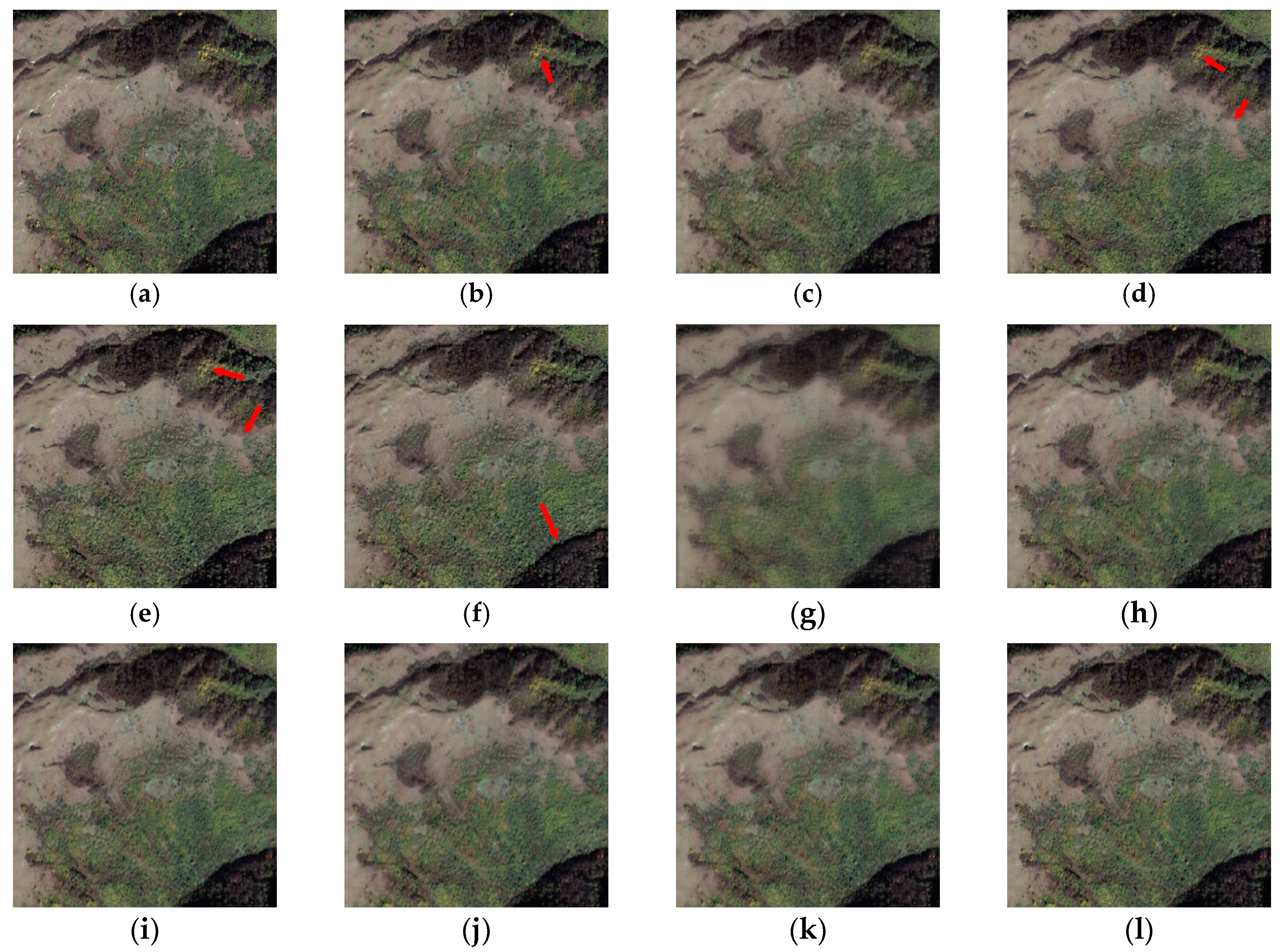
In addition to the quantitative evaluation of the fusion image quality of the algorithm using the evaluation indexes above, the fused image generated by all algorithms is further visualized to check the spectral distortion or spatial distortion that may be generated by various algorithms. Since the size of the real data image is large, it is difficult to distinguish the subtle differences between different fused images by the naked eye. This paper begins with the IKONOS dataset. Figure 4 shows the fused images generated by various algorithms for the fusion of a set of images in the INONOS test set.
As shown in Figure 4, the selected image is a mountain scene where all MS images are synthesized into true color images by their red, green, and blue bands. Figure 4a shows the high spatial resolution MS image that is the ground truth, and Figure 4b–l show fused images generated by different methods. In Figure 4, it can be seen that all of the methods besides ATWT-M3 can reconstruct a visually satisfactory MS image. The fused image of ATWT-M3 is blurred. The main reason caused the blurring effect of spatial distortion is that the method cannot extract appropriate spatial information from the PAN image and inject it into an MS image. In contrast, by careful observation, the fused image generated by the Indusion method even has more spatial detail than the reference image, which is over-sharpening and is also considered as spatial distortion. The GSA and BDSD methods have different degrees of color difference compared to the reference image, which is more obvious in the flat area of the scene. In contrast, the proposed network, PNN, TFNet, PNN+, DRPNN, PanNet, and MSDCNN can generate fused images with less spatial and spectral distortion than other methods. These fused images are closest to the reference image. It is difficult to distinguish which is better through qualitative evaluation. However, the quantitative evaluations have already demonstrated that the proposed network can perform better.
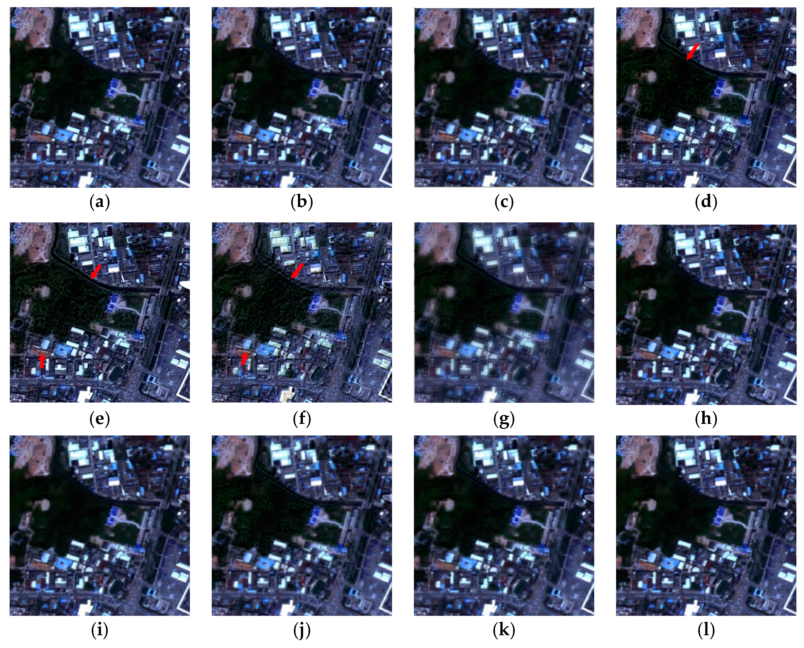
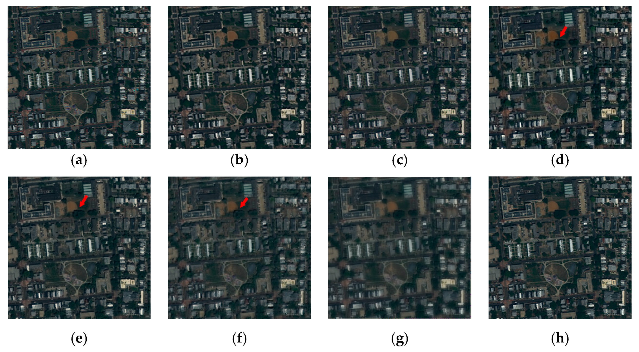
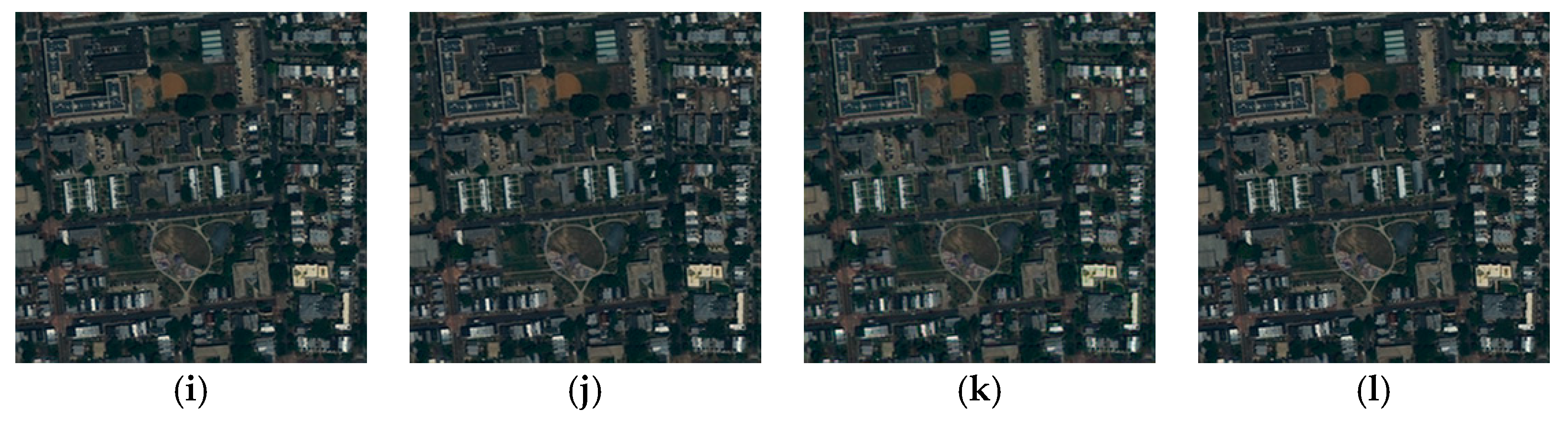
Besides, a set of urban scenes in the GaoFen-2 test set is selected for visual analysis of the fused images generated by algorithms mentioned above. As shown in Figure 5 similar phenomena can be found on the IKONOS test images. Firstly, the fused image of ATWT-M3 is still blurring. The other methods other than CNNs have obvious spatial distortion, which is especially obvious in the darker areas at the center of the scene. The fused images of those methods have a spatial texture that does not exist in the reference image. In addition, the color of some areas in the BDSD’s and GSA’s fused images have a significant difference with the reference image, which is spectral distortion. To summarize, our network and PNN produce fused images with no apparent spectral and spatial distortion relative to the reference image, and the numerical evaluation index indicates that our network has the optimal fusion performance. The visual contrast of the fused image on the WorldView-2 dataset is similar, as shown in Figure 6.
4.5. Discussion
In this section, we further discussed the effect of dense blocks and residual learning in the proposed network. To evaluate the effect of dense blocks, the models with commonly-used residual blocks are tested. For comparison equality, each model has 18 3 × 3 convolutional layers in the fusion module. Therefore, each model has three dense blocks or nine residual blocks. In 3 × 3 convolutional layers of dense blocks, the number of channels is 32, whereas the counterpart of residual blocks is 128. The effect of residual learning is also investigated by removing it from the proposed CNN. We have two conditions (e.g., choice of blocks and whether to use residual learning or not), and each condition has two options. Therefore, we carried out four experiments on each dataset. The batch size is set as 10. The weight decay of the Adam algorithm is 0.001. The initial learning rate was set to 0.001, and it was multiplied by 0.5 per 5000 iterations during training. 12 sets of quantitative evaluation results are shown in Table 10, Table 11 and Table 12. In the tables, the best and the second best results of each index are written in red and blue, respectively.
It is obvious that dense blocks significantly improve the performance of the proposed network. The average Q8, UIQI, SAM, ERGAS, and SCC of dense blocks based networks are 0.6922, 0.8718, 3.8207, 3.3, and 0.9431, whereas the counterparts with residual blocks are 0.6028, 0.8116, 6.1988, 5.3931, and 0.9. From these indexes, it is clear that dense blocks have a significant for improving the performance. Dense connections bring the following advantages. Deep CNNs may be plagued with the vanishing gradient problem, because the large number of layers hinder the transmission of input information and gradient information in the forward and backpropagation of the network. In dense blocks, each layer is directly connected to the input and output of the network, so the transfer of feature information and gradient information in the network will become more effective. Dense blocks enable deep convolutional layers to reuse feature maps generated by shallow convolutional layers to realize full utilization of all feature maps in the block, effectively avoiding vanishing gradient problem. These advantages can help facilitate the training process. In addition, although a large number of feature maps need to be processed in the dense block, the application of the bottleneck layers and the transformation layer greatly reduces the number of computational complexity parameters of the network. In fact, each layer of dense blocks can make use of not only the features generated by the previous layer but also the features generated by all previous layers. The significance of applying dense blocks to MS pansharpening is that feature maps of different depth, abstract degree, and expression ability can be utilized and integrated into a high-efficiency feature map.
It should also be noticed that residual learning has a significant effect on dense block based methods. Six experiments are associated with dense blocks, where three models equipped with residual learning. These models achieve the best results in ten of fifteen indexes. Especially, the UIQI increases by approximately 10% in Table 10. The effect of residual learning is reasonable because input MS images are very similar to reference images. It is quite difficult for the network to reconstruct the desired output directly, but the reconstruction module becomes efficient when it comes to learning the residual between the input and output. The two basic objectives reflected in the fusion of MS images are spectral information preservation and spatial information enhancement. Residual learning directly brings the spectral information of the original MS image of the fused image, while the network is used to generate the missing spatial information in the original MS image. Compared to the general CNN that directly construct the high spatial resolution MS image, the CNN with residual learning has a clear physical interpretation, so learning the residual of input and target is a natural choice for MS pansharpening. In Table 11, the residual blocks based model without residual learning obtains the best result in the UIQI index, which also demonstrates the effect of residual learning. That is because residual learning exists in residual blocks in that model.
Although the proposed network outperforms some state-of-the-art methods, it cannot deny that there are some cases of failure, e.g., the edge of yellow points on the corner of Figure 4b is blurred. The problem is caused by the loss of high frequency information. To struggle against the blurred edges, the high-pass filter can be introduced to describe structural similarity while minimizing spectral distortion. However, the fused MS images may suffer from some degradation due to indecent structural constraints.
5. Conclusions
In this paper, we proposed a very deep CNN with dense blocks and residual learning for MS pansharpening. The proposed network makes use of dense blocks to reuse feature maps, reduce parameters, and facilitate gradient flow during training. These advantages help our network learn the complex nonlinearity mapping relationship effectively, even though the depth of the proposed network reaches 44 learnable layers. We also explored residual learning to boost the performance. It can provide complementary detail information, which can reduce the difficulty of MS image reconstruction. Experiments have been implemented on three datasets and the proposed network achieves competitive or superior performance. We discussed the effect of dense blocks and residual learning. The experiment results show that the model with the designed dense blocks outperforms that with residual blocks, which demonstrates the effectiveness of dense connections. The improvement brought by residual learning illustrates that it can reduce the difficulty of MS image reconstruction and further improve the performance of the proposed network.
In terms of future research, we plan to test the proposed method in other fusion scenarios, e.g., hyperspectral pansharpening and hyperspectral and MS image fusion. In addition, how to extract and fuse spatial and spectral features more effectively remains active research.
Author Contributions
All the authors made significant contributions to this work. D.W. and Y.L. devised the approach and analyzed the data; J.C.-W.C. helped design the experiments and provided advice for the preparation and revision of the work; D.W. and L.M. performed the experiments; and Z.B. helped with the experiments.
Funding
This work was supported by the National Natural Science Foundation of China (61871460, 61761042), the Natural Science Basic Research Plan in Shaanxi Province of China (2018JM6066), the Fundamental Research Funds for the Central Universities (3102019ghxm016), and the Key Research and Development Program of Yanan (2017KG-01,2017WZZ-04-01).
Acknowledgments
The authors would like to thank Qingping Zheng from Northwestern Polytechnical University for providing advices in terms of coding.
Conflicts of Interest
The authors declare no competing financial interests. The founding sponsors had no role in the design of the study; in the collection, analyses, or interpretation of data; in the writing of the manuscript; and in the decision to publish the results.
References
- Karoui, M.S.; Benhalouche, F.Z.; Deville, Y.; Djerriri, K.; Briottet, X.; Houet, T.; Le Bris, A.; Weber, C. Partial Linear NMF-Based Unmixing Methods for Detection and Area Estimation of Photovoltaic Panels in Urban Hyperspectral Remote Sensing Data. Remote Sens. 2019, 11, 2164. [Google Scholar] [CrossRef]
- Garzelli, A.; Aiazzi, B.; Alparone, L.; Lolli, S.; Vivone, G. Multispectral Pansharpening with Radiative Transfer-Based Detail-Injection Modeling for Preserving Changes in Vegetation Cover. Remote. Sens. 2018, 10, 1308. [Google Scholar] [CrossRef]
- Wang, P.; Wang, L.; Wu, Y.; Leung, H. Utilizing Pansharpening Technique to Produce Sub-Pixel Resolution Thematic Map from Coarse Remote Sensing Image. Remote. Sens. 2018, 10, 884. [Google Scholar] [CrossRef]
- Souza, C., Jr.; Firestone, L.; Silva, L.M.; Roberts, D. Mapping forest degradation in the Eastern Amazon from SPOT 4 through spectral mixture models. Remote Sens. Environ. 2003, 87, 494–506. [Google Scholar] [CrossRef]
- Mohammadzadeh, A.; Tavakoli, A.; Zoej, M.J.V. Road extraction based on fuzzy logic and mathematical morphology from pan—Sharpened ikonos images. Photogramm. Record 2010, 21, 44–60. [Google Scholar] [CrossRef]
- Fang, B.; Li, Y.; Zhang, H.; Chan, J.C. Hyperspectral Images Classification Based on Dense Convolutional Networks with Spectral-Wise Attention Mechanism. Remote Sens. 2019, 11, 159. [Google Scholar] [CrossRef]
- Amro, I.; Mateos, J.; Vega, M.; Molina, R.; Katsaggelos, A.K. A survey of classical methods and new trends in pansharpening of multispectral images. Eurasip J. Adv. Signal Process. 2011, 2011, 79. [Google Scholar] [CrossRef] [Green Version]
- Aiazzi, B.; Baronti, S.; Selva, M. Improving Component Substitution Pansharpening through Multivariate Regression of MS +Pan Data. IEEE Trans. Geosci. Remote Sens. 2007, 45, 3230–3239. [Google Scholar] [CrossRef]
- Xie, B.; Zhang, H.; Huang, B. Revealing implicit assumptions of the component substitution pansharpening methods. Remote Sens. 2017, 9, 443. [Google Scholar] [CrossRef]
- Garzelli, A.; Nencini, F.; Capobianco, L. Optimal MMSE Pan Sharpening of Very High Resolution Multispectral Images. IEEE Trans. Geosci. Remote Sens. 2007, 46, 228–236. [Google Scholar] [CrossRef]
- Khan, M.M.; Chanussot, J.; Condat, L.; Montanvert, A. Indusion: Fusion of Multispectral and Panchromatic Images Using Induction Scaling Technique. IEEE Geosci. Remote Sens. Lett. 2008, 5, 98–102. [Google Scholar] [CrossRef]
- Ranchin, T.; Aiazzi, B.; Alparone, L.; Baronti, S.; Wald, L. Image fusion—The ARSIS concept and some successful implementation schemes. Isprs J. Photogram. Remote Sens. 2003, 58, 4–18. [Google Scholar] [CrossRef]
- Palsson, F.; Ulfarsson, M.O.; Sveinsson, J.R. Model-Based Reduced-Rank Pansharpening. IEEE Geosci. Remote. Sens. Lett. 2019. [Google Scholar] [CrossRef]
- Choi, J.; Kim, G.; Park, N.; Park, H.; Choi, S. A hybrid pansharpening algorithm of VHR satellite images that employs injection gains based on NDVI to reduce computational costs. Remote Sens. 2017, 9, 976. [Google Scholar] [CrossRef]
- Choi, J.; Park, H.; Seo, D. Pansharpening Using Guided Filtering to Improve the Spatial Clarity of VHR Satellite Imagery. Remote Sens. 2019, 11, 633. [Google Scholar] [CrossRef]
- Lillo-Saavedra, M.; Gonzalo-Martín, C.; García-Pedrero, A.; Lagos, O. Scale-aware pansharpening algorithm for agricultural fragmented landscapes. Remote Sens. 2016, 8, 870. [Google Scholar] [CrossRef]
- Masi, G.; Cozzolino, D.; Verdoliva, L.; Scarpa, G. Pansharpening by convolutional neural networks. Remote Sens. 2016, 8, 594. [Google Scholar] [CrossRef]
- Jiang, Z.; Yuan, Y.; Wang, Q. Contour-aware network for semantic segmentation via adaptive depth. Neurocomputing 2018, 284, 27–35. [Google Scholar] [CrossRef]
- Dong, C.; Loy, C.C.; He, K.; Tang, X. Image super-resolution using deep convolutional networks. IEEE Trans. Pattern Anal. Mach. Intell. 2015, 38, 295–307. [Google Scholar] [CrossRef]
- Yuan, Q.; Wei, Y.; Meng, X.; Shen, H.; Zhang, L. A multiscale and multidepth convolutional neural network for remote sensing imagery pan-sharpening. IEEE J. Sel. Top. Appl. Earth Obs. Remote. Sens. 2018, 11, 978–989. [Google Scholar] [CrossRef]
- Liu, X.; Liu, Q.; Wang, Y. Remote sensing image fusion based on two-stream fusion network. Inf. Fusion 2020, 55, 1–15. [Google Scholar] [CrossRef]
- Krizhevsky, A.; Sutskever, I.; Hinton, G.E. ImageNet Classification with Deep Convolutional Neural Networks. In Proceedings of the International Conference on Neural Information Processing Systems, Lake Tahoe, NV, USA, 3–6 December 2012. [Google Scholar]
- Simonyan, K.; Zisserman, A. Very deep convolutional networks for large-scale image recognition. arXiv 2014, preprint. arXiv:1409.1556. [Google Scholar]
- Szegedy, C.; Liu, W.; Jia, Y.; Sermanet, P.; Reed, S.; Anguelov, D.; Erhan, D.; Vanhoucke, V.; Rabinovich, A. Going deeper with convolutions. In Proceedings of the IEEE Conference on Computer Vision and Pattern Recognition, Boston, MA, USA, 8–10 June 2015. [Google Scholar]
- He, K.; Zhang, X.; Ren, S.; Sun, J. Deep residual learning for image recognition. In Proceedings of Proceedings of the IEEE Conference on Computer Vision and Pattern Recognition, Las Vegas, NV, USA, 27–30 June 2016. [Google Scholar]
- Huang, G.; Liu, Z.; Van Der Maaten, L.; Weinberger, K.Q. Densely connected convolutional networks. In Proceedings of the IEEE Conference on Computer Vision and Pattern Recognition, Honolulu, HI, USA, 21–26 July 2017. [Google Scholar]
- Gangkofner, U.G.; Pradhan, P.S.; Holcomb, D.W. Optimizing the high-pass filter addition technique for image fusion. Photogramm. Eng. Remote Sens. 2007, 73, 1107–1118. [Google Scholar] [CrossRef]
- Rubinstein, R.; Bruckstein, A.M.; Elad, M. Dictionaries for sparse representation modeling. Proceed. IEEE 2010, 98, 1045–1057. [Google Scholar] [CrossRef]
- Kreutz-Delgado, K.; Murray, J.F.; Rao, B.D.; Engan, K.; Lee, T.W.; Sejnowski, T.J. Dictionary learning algorithms for sparse representation. Neural Comput. 2003, 15, 349–396. [Google Scholar] [CrossRef]
- Li, S.; Yang, B. A New Pan-Sharpening Method Using a Compressed Sensing Technique. IEEE Trans. Geosci. Remote Sens. 2011, 49, 738–746. [Google Scholar] [CrossRef]
- Cheng, J.; Zhang, H.; Shen, H.; Zhang, L. A Practical Compressed Sensing-Based Pan-Sharpening Method. IEEE Geosci. Remote Sens. Lett. 2012, 9, 629–633. [Google Scholar] [CrossRef]
- Xiao, X.Z.; Bamler, R. A Sparse Image Fusion Algorithm with Application to Pan-Sharpening. IEEE Trans. Geosci. Remote Sens. 2013, 51, 2827–2836. [Google Scholar]
- Zhong, S.; Ye, Z.; Chen, Y.; Di, W. Combining Component Substitution and Multiresolution Analysis: A Novel Generalized BDSD Pansharpening Algorithm. IEEE J. Sel. Top. Appl. Earth Obs. Remote. Sens. 2017, 10, 2867–2875. [Google Scholar] [CrossRef]
- Scarpa, G.; Vitale, S.; Cozzolino, D. Target-adaptive CNN-based pansharpening. IEEE Trans. Geosci. Remote Sens. 2018, 56, 5443–5457. [Google Scholar] [CrossRef]
- Wei, Y.; Yuan, Q.; Shen, H.; Zhang, L. Boosting the accuracy of multispectral image pansharpening by learning a deep residual network. IEEE Geosci. Remote Sens. Lett. 2017, 14, 1795–1799. [Google Scholar] [CrossRef]
- Yang, J.; Fu, X.; Hu, Y.; Huang, Y.; Ding, X.; Paisley, J. PanNet: A deep network architecture for pan-sharpening. In Proceedings of the IEEE International Conference on Computer Vision, Venice, Italy, 22–29 October 2017. [Google Scholar]
- Lim, B.; Son, S.; Kim, H.; Nah, S.; Lee, K.M. Enhanced Deep Residual Networks for Single Image Super-Resolution. In Proceedings of the Computer Vision & Pattern Recognition Workshops, Honolulu, HI, USA, 21–26 July 2017. [Google Scholar]
- Ioffe, S.; Szegedy, C. Batch normalization: Accelerating deep network training by reducing internal covariate shift. arXiv 2015, preprint. arXiv:1502.03167. [Google Scholar]
- Zeiler, M.D.; Taylor, G.W.; Fergus, R. Adaptive deconvolutional networks for mid and high level feature learning. In Proceedings of the IEEE International Conference on Computer Vision, Barcelona, Spain, 6–13 November 2018. [Google Scholar]
- Wald, L.; Ranchin, T.; Marc, M. Fusion of satellite images of different spatial resolutions: Assessing the quality of resulting images. Photogramm. Eng. Remote Sens. 1997, 63, 691–699. [Google Scholar]
- Dennison, P.E.; Halligan, K.Q.; Roberts, D.A. A comparison of error metrics and constraints for multiple endmember spectral mixture analysis and spectral angle mapper. Remote Sens. Environ. 2004, 93, 359–367. [Google Scholar] [CrossRef]
- Zhou, J.; Civco, D.L.; Silander, J.A. A wavelet transform method to merge Landsat TM and SPOT panchromatic data. Int. J. Remote Sens. 1998, 19, 743–757. [Google Scholar] [CrossRef]
- Ayhan, E. Spectral and Spatial Quality Analysis in Pan Sharpening Process. J. Indian Soc. Remote Sens. 2012, 40, 379–388. [Google Scholar] [CrossRef]
- Wang, Z.; Bovik, A.C. A universal image quality index. IEEE Signal Process. Lett. 2002, 9, 81–84. [Google Scholar] [CrossRef]
- Zeng, Y.; Huang, W.; Liu, M.; Zhang, H.; Zou, B. Fusion of satellite images in urban area: Assessing the quality of resulting images. In Proceedings of the 2010 18th International Conference on Geoinformatics, Beijing, China, 18–20 June 2010. [Google Scholar]
- Garzelli, A.; Nencini, F. Hypercomplex Quality Assessment of Multi/Hyperspectral Images. IEEE Geosci. Remote Sens. Lett. 2009, 6, 662–665. [Google Scholar] [CrossRef]
Figure 1.
A schematic diagram of multispectral pansharpening.

Figure 2.
The detailed architecture of the proposed network.

Figure 3.
The structure of dense blocks used in the feature fusion module. Original cuboids represent convolutional layers. The 128 and 32 below cuboids represent the number of channels.
Figure 3.
The structure of dense blocks used in the feature fusion module. Original cuboids represent convolutional layers. The 128 and 32 below cuboids represent the number of channels.

Figure 4.
Fused images of different methods on IKONOS dataset. (a) ground truth; (b) our model; (c) PNN; (d) BDSD; (e) GSA; (f) Indusion; (g) ATWT-M3; (h) TFNet; (i) PNN+; (j) DRPNN; (k) PanNet; and (l) MSDCNN.
Figure 4.
Fused images of different methods on IKONOS dataset. (a) ground truth; (b) our model; (c) PNN; (d) BDSD; (e) GSA; (f) Indusion; (g) ATWT-M3; (h) TFNet; (i) PNN+; (j) DRPNN; (k) PanNet; and (l) MSDCNN.

Figure 5.
Fused images of different methods on GaoFen-2 dataset. (a) ground truth; (b) our model; (c) PNN; (d) BDSD; (e) GSA; (f) Indusion; (g) ATWT-M3; (h) TFNet; (i) PNN+; (j) DRPNN; (k) PanNet; and (l) MSDCNN.
Figure 5.
Fused images of different methods on GaoFen-2 dataset. (a) ground truth; (b) our model; (c) PNN; (d) BDSD; (e) GSA; (f) Indusion; (g) ATWT-M3; (h) TFNet; (i) PNN+; (j) DRPNN; (k) PanNet; and (l) MSDCNN.

Figure 6.
Fused images of different methods on WorldView-2 dataset. (a) ground truth; (b) our model; (c) PNN; (d) BDSD; (e) GSA; (f) Indusion; (g) ATWT-M3; (h) TFNet; (i) PNN+; (j) DRPNN; (k) PanNet; and (l) MSDCNN.
Figure 6.
Fused images of different methods on WorldView-2 dataset. (a) ground truth; (b) our model; (c) PNN; (d) BDSD; (e) GSA; (f) Indusion; (g) ATWT-M3; (h) TFNet; (i) PNN+; (j) DRPNN; (k) PanNet; and (l) MSDCNN.


Table 1.
Spatial resolution and wavelength range of each band of IKONOS satellite imagery.
| Band | Spatial Resolution (m) | Wavelength Range (nm) | Remark |
|---|---|---|---|
| 1 | 4 | 450–530 | blue |
| 2 | 4 | 520–610 | green |
| 3 | 4 | 640–720 | red |
| 4 | 4 | 760–860 | near-infrared |
| PAN | 1 | 450–900 |
Table 2.
Spatial resolution and wavelength range of each band of GaoFen-2 satellite imagery.
| Band | Spatial Resolution (m) | Wavelength Range (nm) | Remark |
|---|---|---|---|
| 1 | 4 | 450–520 | blue |
| 2 | 4 | 520–590 | green |
| 3 | 4 | 630–690 | red |
| 4 | 4 | 770–890 | near-infrared |
| PAN | 1 | 450–900 |
Table 3.
Spatial resolution and wavelength range of each band of WorldView-2 satellite imagery.
| Band | Spatial Resolution (m) | Wavelength Range (nm) | Remark |
|---|---|---|---|
| 1 | 2 | 400–450 | Coastal |
| 2 | 2 | 450–510 | Blue |
| 3 | 2 | 510–580 | green |
| 4 | 2 | 585–625 | yellow |
| 5 | 2 | 630–690 | red |
| 6 | 2 | 705–745 | Red edge |
| 7 | 2 | 770–895 | Near-IR1 |
| 8 | 2 | 860–1040 | Near-IR2 |
| PAN | 0.5 | 450–800 |
Table 4.
The distribution of images for training, validation, and testing.
| Dataset | Train Set | Validation Set | Test Set |
|---|---|---|---|
| IKONOS | 400 | 100 | 50 |
| GaoFen-2 | 400 | 100 | 50 |
| WorldView-2 | 400 | 100 | 50 |
Table 5.
The results of the proposed network on the train set, validation set, and test set.
| Dataset | Q4 | UIQI | SAM | ERGAS | SCC | |
|---|---|---|---|---|---|---|
| IKONOS | train set | 0.6906 | 0.9081 | 3.5662 | 2.8386 | 0.9265 |
| validation set | 0.7067 | 0.9377 | 4.0377 | 3.1634 | 0.9528 | |
| test set | 0.6897 | 0.9124 | 3.8708 | 3.0361 | 0.9278 | |
| GaoFen-2 | train set | 0.7873 | 0.9576 | 2.6356 | 3.8959 | 0.9282 |
| validation set | 0.7941 | 0.9710 | 2.7285 | 4.0443 | 0.9329 | |
| test set | 0.7878 | 0.9579 | 2.6491 | 3.7303 | 0.9293 | |
| WorldView-2 | train set | 0.6987 | 0.9296 | 5.2454 | 3.3422 | 0.9496 |
| validation set | 0.7170 | 0.8996 | 5.1448 | 3.4071 | 0.9501 | |
| test set | 0.6659 | 0.9174 | 5.0045 | 3.1758 | 0.9514 | |
Table 6.
The number of learnable layers of different convolutional neural networks (CNNs) for pansharpening.
Table 6.
The number of learnable layers of different convolutional neural networks (CNNs) for pansharpening.
| Method | PNN [17] | PNN+ [34] | MSDCNN [20] | DRPNN [35] | TFNet [21] | PanNet [36] | The proposed network |
| The number of learnable layers | 3 | 3 | 5 | 11 | 18 | 21 | 44 |
Table 7.
Quantitative evaluation results of different methods on the IKONOS dataset. The best and the second best results are in red and blue, respectively.
Table 7.
Quantitative evaluation results of different methods on the IKONOS dataset. The best and the second best results are in red and blue, respectively.
| Methods | Q4 | UIQI | SAM | ERGAS | SCC |
|---|---|---|---|---|---|
| BDSD [10] | 0.5279 | 0.8316 | 5.0190 | 4.6855 | 0.7592 |
| GSA [8] | 0.5384 | 0.8256 | 5.0036 | 4.7029 | 0.7545 |
| Indusion [11] | 0.4927 | 0.7942 | 5.2510 | 5.0797 | 0.7499 |
| ATWT-M3 [12] | 0.3553 | 0.7866 | 4.9390 | 4.7348 | 0.7542 |
| PNN [17] | 0.5474 | 0.8458 | 4.9105 | 4.2016 | 0.8010 |
| PNN+ [34] | 0.5518 | 0.8599 | 4.2989 | 3.9579 | 0.8173 |
| DRPNN [35] | 0.5320 | 0.8465 | 4.5075 | 4.1639 | 0.8055 |
| PanNet [36] | 0.5293 | 0.8393 | 4.7777 | 4.2836 | 0.8014 |
| TFNet [21] | 0.6592 | 0.8964 | 4.1303 | 3.3761 | 0.9186 |
| MSDCNN [20] | 0.5683 | 0.8686 | 4.1819 | 3.7883 | 0.8328 |
| Our model | 0.6897 | 0.9124 | 3.8708 | 3.0361 | 0.9278 |
Table 8.
Quantitative evaluation results of different methods on the GaoFen-2 dataset. The best and the second best results are in red and blue, respectively.
Table 8.
Quantitative evaluation results of different methods on the GaoFen-2 dataset. The best and the second best results are in red and blue, respectively.
| Methods | Q4 | UIQI | SAM | ERGAS | SCC |
|---|---|---|---|---|---|
| BDSD [10] | 0.6358 | 0.7941 | 6.4198 | 7.4680 | 0.7746 |
| GSA [8] | 0.6374 | 0.7838 | 6.7213 | 7.7009 | 0.7589 |
| Indusion [11] | 0.6086 | 0.7134 | 7.0485 | 9.2282 | 0.7090 |
| ATWT-M3 [12] | 0.5625 | 0.8313 | 5.3411 | 6.4143 | 0.7955 |
| PNN [17] | 0.7390 | 0.9094 | 4.3010 | 4.3037 | 0.8776 |
| PNN+ [34] | 0.7843 | 0.9488 | 3.0594 | 3.5287 | 0.9092 |
| DRPNN [35] | 0.7275 | 0.8719 | 4.6670 | 4.8960 | 0.8515 |
| PanNet [36] | 0.7504 | 0.9008 | 4.1774 | 4.4150 | 0.8752 |
| TFNet [21] | 0.6907 | 0.9164 | 3.7689 | 3.9698 | 0.9139 |
| MSCDNN [20] | 0.8031 | 0.9507 | 3.0032 | 3.2756 | 0.9213 |
| Our model | 0.7878 | 0.9579 | 2.6491 | 3.7303 | 0.9293 |
Table 9.
Quantitative evaluation results of different methods on the WorldView-2 dataset. The best and the second best results are in red and blue, respectively.
Table 9.
Quantitative evaluation results of different methods on the WorldView-2 dataset. The best and the second best results are in red and blue, respectively.
| Methods | Q8 | UIQI | SAM | ERGAS | SCC |
|---|---|---|---|---|---|
| BDSD [10] | 0.5274 | 0.8113 | 9.3758 | 5.5981 | 0.8124 |
| GSA [8] | 0.5360 | 0.8504 | 7.6713 | 4.6466 | 0.8317 |
| Indusion [11] | 0.4933 | 0.8322 | 7.4204 | 4.9532 | 0.8292 |
| ATWT-M3 [12] | 0.2772 | 0.7745 | 7.8102 | 5.5833 | 0.8040 |
| PNN [17] | 0.5520 | 0.8717 | 7.0039 | 4.1212 | 0.8709 |
| PNN+ [34] | 0.6209 | 0.9027 | 5.6871 | 3.4700 | 0.9116 |
| DRPNN [35] | 0.6399 | 0.9025 | 5.6503 | 3.3753 | 0.9226 |
| PanNet [36] | 0.5604 | 0.8740 | 6.9058 | 4.1172 | 0.8742 |
| TFNet [21] | 0.6587 | 0.9107 | 5.3367 | 3.3563 | 0.9180 |
| MSDCNN [20] | 0.6628 | 0.9124 | 5.3072 | 3.1768 | 0.9303 |
| Our model | 0.6659 | 0.9174 | 5.0045 | 3.1758 | 0.9514 |
Table 10.
Quantitative evaluation results of different architectures on the IKONOS dataset. The best and the second best results are in red and blue, respectively.
Table 10.
Quantitative evaluation results of different architectures on the IKONOS dataset. The best and the second best results are in red and blue, respectively.
| Residual Learning | Block | Q4 | UIQI | SAM | ERGAS | SCC |
|---|---|---|---|---|---|---|
| without | residual | 0.5320 | 0.7485 | 5.2104 | 5.2364 | 0.8148 |
| with | residual | 0.5644 | 0.8363 | 4.5532 | 4.8801 | 0.9206 |
| without | dense | 0.6527 | 0.8388 | 3.7446 | 3.3091 | 0.8985 |
| with | dense | 0.6571 | 0.9193 | 3.1302 | 3.1413 | 0.9581 |
Table 11.
Quantitative evaluation results of different architectures on the GaoFen-2 dataset. The best and the second best results are in red and blue, respectively.
Table 11.
Quantitative evaluation results of different architectures on the GaoFen-2 dataset. The best and the second best results are in red and blue, respectively.
| Residual Learning | Block | Q4 | UIQI | SAM | ERGAS | SCC |
|---|---|---|---|---|---|---|
| without | residual | 0.7011 | 0.9192 | 4.6839 | 5.8052 | 0.9161 |
| with | residual | 0.6913 | 0.8273 | 4.7060 | 5.9202 | 0.9343 |
| without | dense | 0.7817 | 0.8913 | 2.3748 | 3.2493 | 0.9541 |
| with | dense | 0.7818 | 0.9093 | 2.4477 | 3.3952 | 0.9661 |
Table 12.
Quantitative evaluation results of different architectures on the WorldView-2 dataset. The best and the second best results are in red and blue, respectively.
Table 12.
Quantitative evaluation results of different architectures on the WorldView-2 dataset. The best and the second best results are in red and blue, respectively.
| Residual Learning | Block | Q8 | UIQI | SAM | ERGAS | SCC |
|---|---|---|---|---|---|---|
| without | residual | 0.5931 | 0.7560 | 7.9767 | 4.6968 | 0.8972 |
| with | residual | 0.5347 | 0.7823 | 10.0624 | 5.8198 | 0.9171 |
| without | dense | 0.6665 | 0.8276 | 5.3514 | 3.2424 | 0.9527 |
| with | dense | 0.5972 | 0.9167 | 5.1134 | 3.2669 | 0.9728 |
© 2019 by the authors. Licensee MDPI, Basel, Switzerland. This article is an open access article distributed under the terms and conditions of the Creative Commons Attribution (CC BY) license (http://creativecommons.org/licenses/by/4.0/).
Share and Cite
MDPI and ACS Style
Wang, D.; Li, Y.; Ma, L.; Bai, Z.; Chan, J.C.-W. Going Deeper with Densely Connected Convolutional Neural Networks for Multispectral Pansharpening. Remote Sens. 2019, 11, 2608. https://doi.org/10.3390/rs11222608
AMA Style
Wang D, Li Y, Ma L, Bai Z, Chan JC-W. Going Deeper with Densely Connected Convolutional Neural Networks for Multispectral Pansharpening. Remote Sensing. 2019; 11(22):2608. https://doi.org/10.3390/rs11222608
Chicago/Turabian StyleWang, Dong, Ying Li, Li Ma, Zongwen Bai, and Jonathan Cheung-Wai Chan. 2019. "Going Deeper with Densely Connected Convolutional Neural Networks for Multispectral Pansharpening" Remote Sensing 11, no. 22: 2608. https://doi.org/10.3390/rs11222608
Note that from the first issue of 2016, this journal uses article numbers instead of page numbers. See further details here.