The Case for a Single Channel Composite Arctic Sea Surface Temperature Algorithm

Department of Physics and Space Science, Royal Military College of Canada, Kingston, ON K7K 7B4, Canada
Remote Sens. 2019, 11(20), 2393; https://doi.org/10.3390/rs11202393
Submission received: 13 September 2019
/
Revised: 13 October 2019
/
Accepted: 14 October 2019
/
Published: 16 October 2019
(This article belongs to the Special Issue Polar Sea Ice: Detection, Monitoring and Modeling)
Abstract
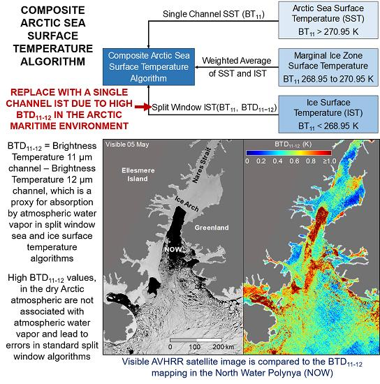
:Surface temperatures derived from satellite thermal infrared (TIR) data are critical inputs for assessing climate change in polar environments. Sea and ice surface temperature (SST, IST) are commonly determined with split window algorithms that use the brightness temperature from the 11 μm channel (BT11) as the main estimator and the difference between BT11 and the 12 μm channel (BTD11–12) to correct for atmospheric water vapor absorption. An issue with this paradigm in the Arctic maritime environment is the occurrence of high BTD11–12 that is not indicative of atmospheric absorption of BT11 energy. The Composite Arctic Sea Surface Temperature Algorithm (CASSTA) considers three regimes based on BT11 pixel value: seawater, ice, and marginal ice zones. A single channel (BT11) estimator is used for SST and a split window algorithm for IST. Marginal ice zone temperature is determined with a weighted average between the SST and IST. This study replaces the CASSTA split window IST with a single channel (BT11) estimator to reduce errors associated with BTD11–12 in the split window algorithm. The single channel IST returned improved results in the CASSTA dataset with a mean average error for ice and marginal ice zones of 0.142 K and 0.128 K, respectively.

1. Introduction
The determination of high latitude surface temperatures is an important factor in assessing climate change in polar environments [1,2,3,4,5,6]. This is particularly true in the Arctic where surface air temperatures are increasing more rapidly than the global average [7,8]. As Arctic waters become less congested with ice during the melt season, there is a rise in the complexity of the thermal mapping of these regions. For the Arctic maritime environment, it is critical to assess sea surface temperature (SST), ice surface temperature (IST), as well as the temperature of marginal ice zones that have a mixture of both ice and water. The paucity of in situ surface temperature measurements in the Arctic is compensated by satellites that collect thermal infrared (TIR) data. Polar orbiting satellites equipped with TIR sensors pass over the polar regions approximately 14 times a day and can provide accurate surface temperatures over large areas. Satellite TIR sensors include the Advanced Very High Resolution Radiometer (AVHRR) carried on the National Oceanic and Atmospheric Administration (NOAA) polar orbiters up to NOAA-19 and the European Space Agency MetOp series, the Moderate Resolution Imaging Spectroradiometer (MODIS) onboard the Aqua and Terra satellites, the Visible Infrared Imager Radiometer Suite (VIIRS) used on the Suomi National Polar-orbiting Partnership (S-NPP) and NOAA-20 satellites, and the Thermal Infrared Sensor (TIRS) on LandSat-8. The combination of datasets from AVHRR (available since 1978), MODIS (available since 1999), VIIRS (available since 2011), and TIRS (available since 2013) allow researchers to assess the effects of climate change in the Arctic. Table 1 lists characteristics of selected satellite TIR sensors.
The determination of SSTs with satellite TIR is well established between 60° N and 60° S latitude with validated accuracies better than 0.5 °C in cloud-free environments [9]. Split window SST algorithms use the brightness temperature from the 11 μm channel (BT11) as the main estimator and the brightness temperature difference between BT11 and the 12 μm channel (BT12), or BTD11–12, to approximate the amount of TIR absorption owing to water vapor in the atmosphere [10]. The split window approach is also commonly used in IST retrieval with observed root-mean-square errors of 1.2 °C or less [11,12,13]. ISTs are generally less accurate than SSTs because ice and snow surfaces are less homogeneous than seawater with respect to emissivity in the 10 μm to 13 μm regime.
In temperate regions, BTD11–12 increases with increasing atmospheric water vapor [14], but there is a progressively weaker association between BTD11–12 and absorption from atmospheric water vapor with increasing latitude [15,16,17]. For Arctic seawater, split window algorithms designed for temperate waters typically overestimate SSTs in the dry arctic atmosphere where high BTD11–12 values are the result of enhanced absorption of BT12 energy by atmospheric ice crystals [18]. Vincent et al. [18,19] demonstrated that there was no correlation between atmospheric absorption and BTD11–12 in the determination of Arctic SSTs as a result of the random orientation and size of ice crystals in the polar atmosphere. This principle also applies to the retrieval of IST in high latitude maritime regions.
The Composite Arctic Sea Surface Temperature Algorithm (CASSTA) was the first satellite algorithm to accurately determine high latitude surface temperature in three different regimes: seawater, ice, and marginal ice zones [18]. CASSTA uses a single channel estimator for Arctic sea surface temperature (ASST), an established split window IST algorithm [20] for ice, and a weighted average of the ASST and IST for marginal ice zones. This paper describes the rationale for using a single channel IST in an Arctic maritime environment and revisits the original CASSTA dataset to determine if the inclusion of a single channel IST returns a more accurate solution.
2. Materials and Methods
2.1. CASSTA
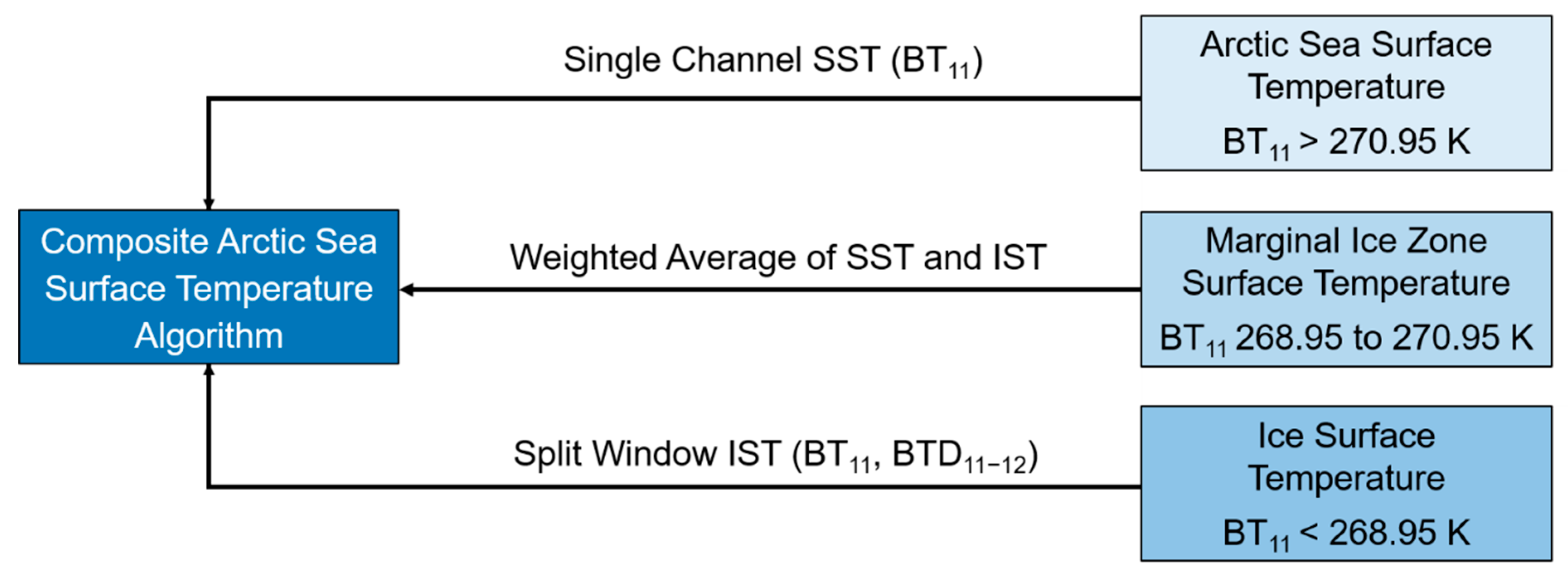
CASSTA was developed in the North Water polynya (NOW) situated between Ellesmere Island and Greenland in northern Baffin Bay at approximately 78°N 74°W. Polynyas are areas of the polar ocean that remain relatively ice-free throughout the year and are good examples of high latitude waters that contain seawater, ice, and marginal ice zones. As part of the NOW Research Network in 1998, the Royal Military College of Canada operated an AVHRR receiving station at Canadian Forces Station Alert on the northern tip of Ellesmere Island. Between 10 March and 2 August 1440 NOAA-12 images were acquired of the NOW region. During this period, the Marine-Atmosphere Emitted Radiance Interferometer (M-AERI) was deployed in the NOW onboard the Canadian Coast Guard Ship Pierre Radisson. The M-AERI is a shipborne IR radiometric interferometer mounted topside of the ship that is capable of measuring in situ SSTs with an accuracy of 0.1 K [21]. The availability of concurrent AVHRR and in situ data in an Arctic maritime environment represented a unique dataset and allowed the development of CASSTA, which considers three different regimes based on the BT11 value of a pixel: seawater, ice, and marginal ice zones (Figure 1). A full description of CASSTA is given in Vincent et al. [18].
2.1.1. Split Window Algorithms
Split window algorithms take the form,
where a, b, c, and d are coefficients normally derived from a linear regression between concurrent in situ and satellite data, and θ is the sensor zenith angle. The split window algorithm uses the physical property that energy in the 12 μm regime undergoes more absorption than the 11 μm regime as a result of atmospheric water vapor and adds a correction to the main estimator (BT11). The sensor zenith angle term accounts for extended path length through the lower atmosphere leading to additional absorption.
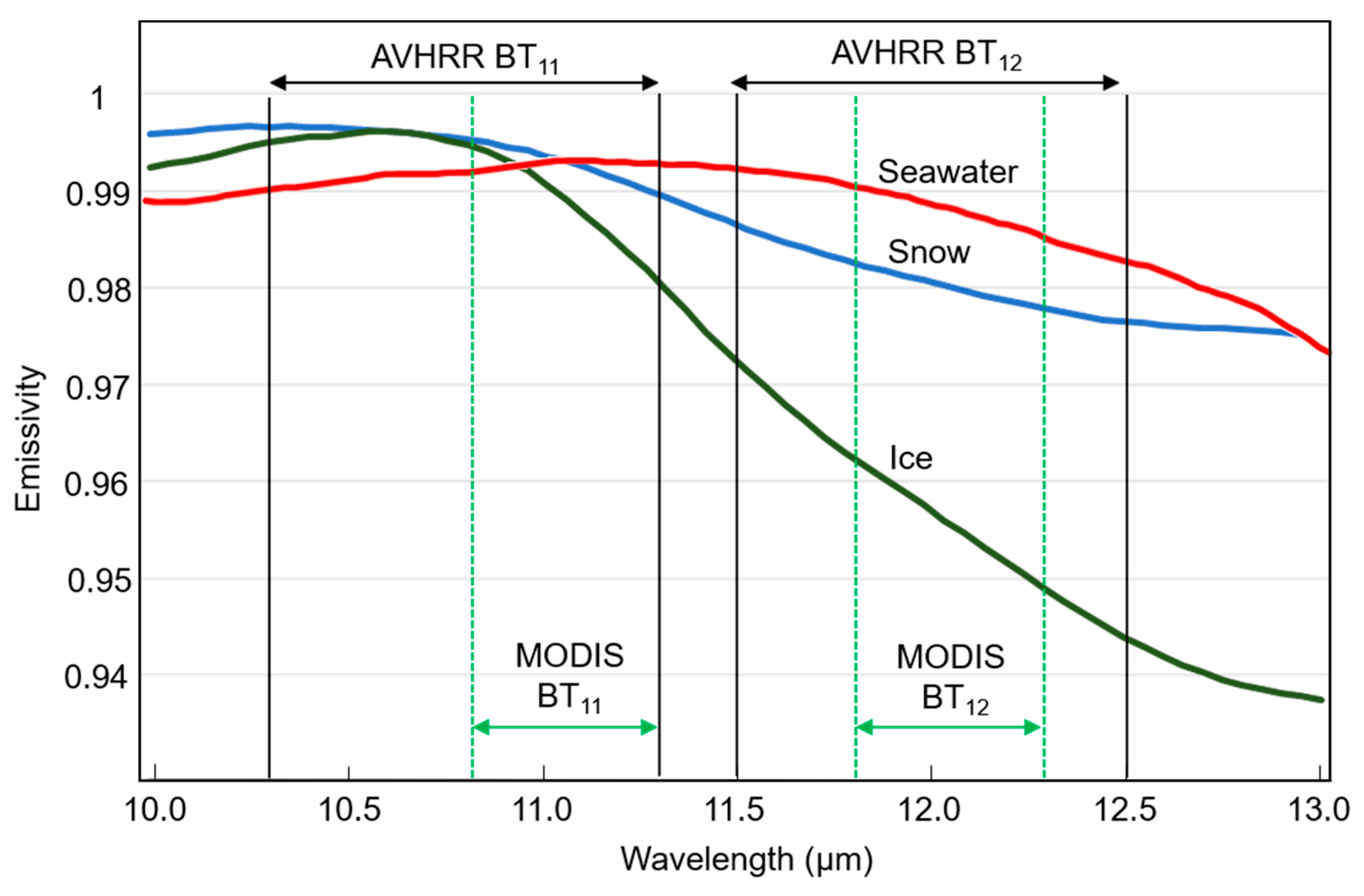
The Pathfinder program, an SST retrieval system developed jointly by the National Aeronautics and Space Administration (NASA) and NOAA, uses a split window nonlinear SST (NLSST) algorithm that includes a first-guess SST estimate to mitigate errors in the BTD11–12 correction. Different coefficients are used for dry regions (BTD11–12 < 0.7 °C) and moist regions (BTD11–12 = 0.7 to 1.0 °C) to improve the fidelity of the algorithm [14]. This system works well for equatorial and temperate waters but is less applicable in the Arctic where high BTD11–12 values are not indicative of atmospheric water vapor. The annual mean distribution of near surface specific humidity, which is considered as a proxy of the vertically integrated water vapor in the atmosphere, is about 18 g kg−1 in equatorial latitudes and decreases to 1 g kg−1 or less in the Arctic [16]. In accordance with the paradigm used for split window SST retrievals, BTD11–12 values in the Arctic should be very low as a result of the relative dryness of the atmosphere, but this is not the case (Figure 2). High BTD11–12 values are observed in Arctic maritime environments, exceeding 1 °C during the colder months and reducing below 1 °C during the summer [19]. One factor is the presence of ice and snow on the surface, both of which have lower emissivity for BT12 wavelengths than BT11 leading to high BTD11–12 values (Figure 3). Another factor is the presence of suspended ice crystals in the Arctic atmosphere that absorb more BT12 energy than water vapor, resulting in elevated values of BTD11–12 when compared to temperate waters [19]. For BTD11–12 values less than 2 K there is little effect on BT11 energy [18,19]. The amount of BT12 absorption is not only dependent on ice crystal concentration but also the shape, size and orientation of the ice crystals [22,23].
2.1.2. Arctic SST
In the development of CASSTA, Vincent et al. [18,19] found no correlation between atmospheric absorption and BTD11–12 in the determination of Arctic SSTs owing to the random orientation and size of ice crystals in the polar atmosphere. A linear regression between 192 concurrent satellite and M-AERI datapoints indicated that a single channel Arctic SST (ASST) algorithm was most applicable where,
The small amount of atmospheric absorption in the BT11 regime is accounted for with the a and b coefficients of the ASST and does not rely on BTD11–12. There is a larger absorption correction for higher ASSTs, which is a function of warmer temperatures leading to increased atmospheric water vapor in the region [11]. Seawater freezes at −1.8 °C, so the ASST is applicable when BT11 for cloud free pixels is greater than 270.95 K [18]. The ASST returned a mean absolute error of 0.186 K with a standard deviation of 0.222 K when compared to the in situ data. By comparison, an established split window NOAA-12 SST algorithm produced an average overestimate of 2.4 K [18].
2.1.3. IST
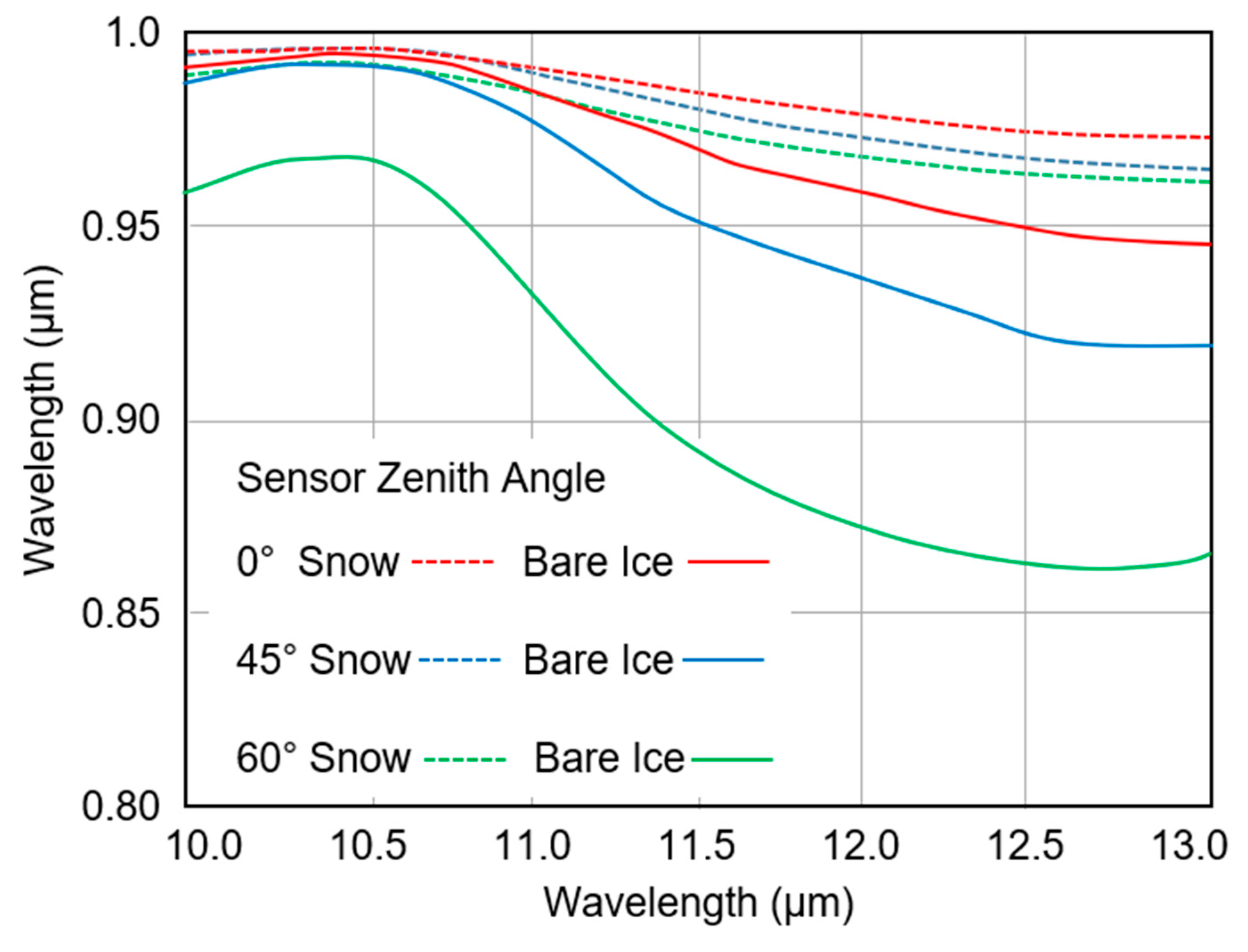
IST retrieval systems commonly use the same split window algorithm as SSTs (Equation (1)) [6]. The determination of IST using satellite thermal data is more complex and generally less accurate than SST because the surface may consist of ice, snow or a combination of the two. The presence of melt ponds during the warmer months may also introduce errors in the calculation. Snow has a higher emissivity than ice in the 10 μm to 13 μm regime, while both surfaces decrease in emissivity in this range (Figure 3). Snow emissivity is also affected by grain size with fine grained snow showing a higher emissivity than coarse grained snow [24]. Another complicating factor is the directional emissivity of snow and ice. Whereas seawater emissivity is relatively constant with respect to sensor zenith angle between 10 μm and 13 μm, snow and ice have decreased emissivity with increasing sensor zenith angle (Figure 4) [25]. The different factors affecting emissivity for IST retrievals lead to solutions that are characteristically less accurate than SST algorithms.
CASSTA uses a split window IST algorithm developed for the NOAA-12 AVHRR [20]. The IST is applicable when BT11 for cloud free pixels is less than 268.95 K [18]. There were only 10 datapoints in this regime that were clustered around 268.5 K, but there was good agreement with the IST which returned a mean absolute error of 0.144 K and a standard deviation of 0.183 K when compared to the in situ data. These results are superior to the published overall accuracy of 0.3 to 2.1 K for the algorithm [20].
2.1.4. Marginal Ice Zone Surface Temperature
The CASSTA dataset included 50 points that fell between the ASST and IST regimes and were designated as marginal ice zone pixels that contained both ice and seawater. Standard regression analysis of these points did not produce a satisfactory result, so a weighted average was used between the ASST and IST BT11 limits of 270.95 K and 268.95 K, respectively. For cloud free pixels that fall in this range, the Marginal Ice Zone Surface Temperature (MIZST) in degrees Celsius is expressed as,
Application of the MIZST resulted in a mean absolute error of 0.136 K with a standard deviation of 0.165 K when compared to the in situ data.
2.2. CASSTA Revisited
2.2.1. IST Reanalysis
The IST used in the development of CASSTA returned good results for the limited number of datapoints, but this should not be true in the general case. If temperate ocean SST algorithms are inaccurate in the Arctic because the BTD11–12 term is not indicative of TIR absorption by atmospheric water vapor, then the same must be true for ISTs that use a split window algorithm in the same maritime environment. The split window IST algorithm was used in CASSTA for two reasons.
- Although it was recognized that BTD11–12 should also affect the IST, the limited number and range of datapoints in the ice regime did not produce a meaningful linear regression. Standard regression analyses for the 50 marginal ice zone points, or a combination of ice and marginal ice zone, were also not successful [18].
- An established IST split window algorithm for NOAA-12 was available [20] and gave unexpected accuracy for the designated ice pixels. Incorporation of the IST algorithm into the MIZST produced good results.
A reanalysis of the CASSTA dataset to incorporate a single channel IST and MIZST solution would require more points in the ice regime to conduct a linear analysis.
2.2.2. New Ice Data
In situ sea ice data was available through the Qaanaaq sea ice thermal emission experiment that took place 30 March to 06 April 2011 on the east side of the NOW [4,26]. Ice temperature was captured by a ground-based SST infrared radiometer (ISAR) using a single channel operating at 9.6 μm to 11.3 μm. ISAR is a self-calibrating radiometer that accounts for sky contribution to provide accurate surface temperatures [27]. Measurements were taken on a near continuous basis at two locations: 77.43ºN 69.14ºW from 01 to 03 April and 77.44ºN 69.27ºW from 03 to 06 April. A total of 14 concurrent ISAR and MetOp-A AVHRR datapoints were collected for cloud free pixels with BT11 ranging from 247.6 K to 252.6 K. Both the Qaanaaq and CASSTA in situ ice data were collected with accurate ground-based radiometers in the NOW region during spring. NOAA-12 was deactivated in 2007, but the BT11 spectral response functions of the NOAA-12 and MetOp-A AVHRR instruments are nearly identical and have been used interchangeably in previous research [4]. The increased number of datapoints and extended temperature range allows a test of the physics behind the rationale of using a single channel estimator for IST in the Arctic maritime environment.
3. Results
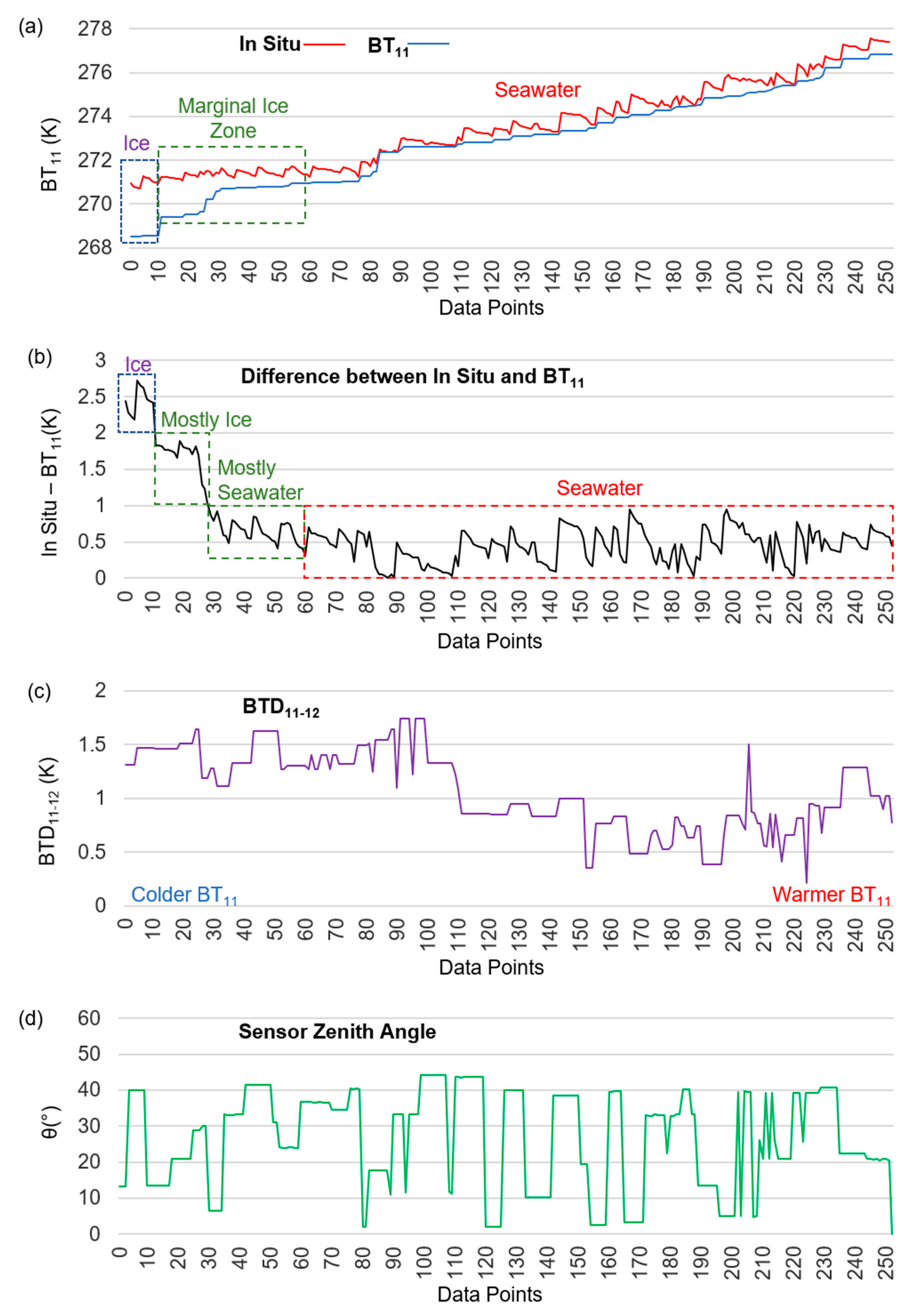
The revision of the CASSTA dataset reveals that the temperature difference between in situ data and BT11 for ice is greater than seawater (Figure 5a). For the ice regime, the in situ data is at least 2.0 K warmer than BT11 with an average of 2.4 K, while seawater averages 0.4 K warmer (Figure 5b). In situ data in the marginal ice zone is 1.1 K warmer on average than BT11. The data implies that the higher differentials between in situ and BT11 values are associated with ice surfaces, which have a lower average emissivity across the AVHRR BT11 band than seawater and snow (Figure 3). A further reduction in the emissivity of ice can be attributable to increasing zenith angle. Colder BT11 values in the CASSTA dataset are generally associated with higher BTD11–12 (Figure 5c), which is likely a function of increased suspended atmospheric ice crystals in cooler air temperatures [19]. There is no relationship between the in situ and BT11 differential with respect to either BTD11–12 or sensor zenith angle (Figure 5d). The reason for this observation is twofold: 1. There is minimal atmospheric absorption; 2. the emissivity of ice decreases marginally for sensor zenith angles less than approximately 50° in the AVHRR BT11 regime.
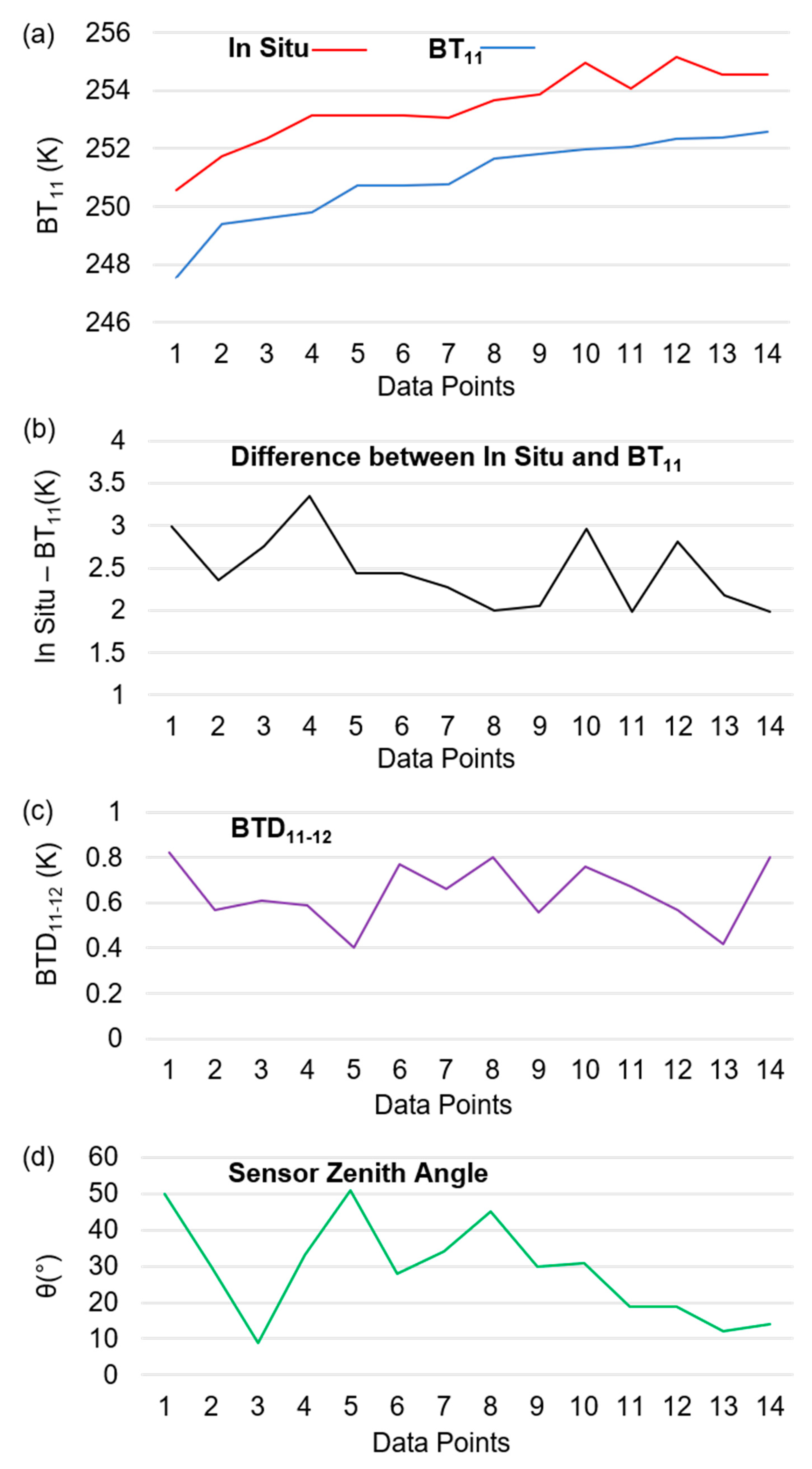
The Qaanaaq ISAR ice data has similar properties to the CASSTA M-AERI dataset (Figure 6). The difference between in situ temperature and BT11 is greater than 2.0 with an average of 2.4 K. BTD11–12 varies between 0.4 K and 0.8 K, with sensor zenith angle ranging from 9° and 51°. Although it is a small sample size, there is no relationship between the in situ and BT11 differential with respect to either BTD11–12 or sensor zenith angle (Figure 6), echoing the CASSTA dataset. These observations give confidence in the addition of these points to the CASSTA ice pixels for the purpose of a linear regression between concurrent in situ and satellite points. As a cross-sensor test, 17 concurrent MODIS BT11 points averaged 2.4 K warmer than Qaanaaq ISAR points with a greater variance than observed for the AVHRR BT11. The increased range of values for MODIS may be attributable to greater variation in ice emissivity for the MODIS BT11 channel (Figure 3).
The M-AERI and ISAR in situ ice temperatures were combined and a linear regression was carried out with the concurrent AVHRR BT11 data, resulting in a correlation coefficient of 0.999 and giving a single channel solution where,
The single channel IST resulted in a mean average error of 0.283 K with a standard deviation of 0.210 K when compared to in situ ice datapoints. By comparison, the split window IST algorithm returned a mean absolute error of 0.965 K with a standard deviation of 0.809 K for the same data. The single channel IST algorithm was then applied only to the CASSTA dataset, changing existing values for both the ice and marginal ice zone regimes. The single channel IST returned improved results in the CASSTA dataset with a mean average error for ice and marginal ice zones of 0.142 K and 0.128 K, respectively. Although the improvements are modest when compared to the original CASSTA dataset (Table 2), the split window IST algorithm used for CASSTA exceeded expected accuracy.
4. Discussion
4.1. Single Channel IST
The viability of a single channel IST algorithm for TIR sensors was examined recently by Liu et al. [6]. The study, which was part of NASA’s Operation IceBridge in northern Alaska, found that that IST retrieval with a single channel had comparable performance to the split window algorithm using VIIRS (Channel M15, 10.26–11.26 μm), with a root-mean-square error of 1.03 K and a bias of 0.22 K. The results showed the IST retrieval biases did not have an apparent dependence on atmospheric water vapor or sensor zenith angle, likely as a result of the dry Arctic climate [6]. Although the research was aimed at finding a solution for satellite imagers that only detect BT11, the atmospheric and surface physics in the Arctic maritime environment, where high BTD11–12 values potentially render split window algorithms less effective, suggest that a single channel solution may be the preferred method. A single channel IST algorithm developed for Landsat-8 (Channel 10, 10.60 μm to 11.19 μm) was shown to be robust to atmospheric water vapor content and returned a root-mean-square error of 0.325 K [28], which further supports the use of BT11 alone for Arctic IST retrieval.
The experiment presented here is meant to examine the physics of the Arctic surface temperature retrieval problem where high BTD11–12 values can lead to erroneous split window values. A further complication is the presence of pixels that contain a mixture of seawater and ice, which is addressed by the CASSTA format. The excellent results obtained in the present study, which are backed by high latitude environmental physics and recent research in the field [6,28], indicate that a single channel CASSTA is applicable for open water and marginal ice zones in the Arctic. Additional concurrent in situ and satellite datapoints, similar to those collected by M-AERI during the initial development of CASSTA, are necessary to create a robust single channel IST algorithm.
4.2. Single Channel CASSTA Considerations
As with all satellite surface temperature algorithms using TIR, cloud-free conditions are necessary for accurate thermal mappings. Clouds prevent the accurate retrieval of surface temperatures for any space based TIR system. The presence of clouds in polar environments is problematic where ice and cloud signatures may be thermally and texturally similar. A feature of the Arctic ocean is the persistence of stratus clouds during the warmer months [29], with July cloud cover potentially exceeding 90% [30]. The difficulty in detection and prominence of clouds in high latitude regions may limit the usefulness of CASSTA. Multichannel analysis using visible, near infrared, and TIR channels help to identify clouds.
Although not used in the temperature calculation, BT12 and sensor zenith angle is useful when using CASSTA. Vincent et al. determined that BTD11–12 > 2.0 °C is indicative of ice fog, which commonly occurs during the colder months in the vicinity of leads [19]. This low-lying feature occurs under apparent clear sky conditions and prevents accurate surface temperature retrieval. If a split window IST is used, the high BTD11–12 in these regions will lead to a warm temperature anomaly owing to the very high BTD11–12 term in the algorithm. Unrealistic results will also occur in cases when BTD11–12 < 0 °C. Negative values of BTD11–12 indicate the presence of mineral dust aerosols in polar regions that may be manifested in optically thin clouds or through deposition on ice and water surfaces [31]. The relatively low emissivity of dust in the BT11 regime compared to seawater or ice will lead to unrealistically cold CASSTA temperatures. Pixels with ice fog or dust should be masked in the CASSTA product. High sensor zenith angles may also produce poor results as a result of decreasing emissivity of ice in the BT11 band. Sensor zenith angles less than 45° will generally yield better results [18]. Liu et al. [6] utilized a solar zenith term in the single channel algorithm to account for enhanced absorption as a result of increased path length, but this term would likely be more useful to account for the reduced emissivity of ice with increasing scan angle. Table 3 summarizes considerations for CASSTA.
5. Conclusions
Developed by Vincent et al. [18], CASSTA identifies three regimes of the Arctic maritime environment based on BT11 values and applies a specific algorithm for seawater, ice, and marginal ice zones. For seawater, the algorithm utilizes a single channel estimator (BT11), while a split window IST algorithm is used for ice. The marginal ice zone uses a weighted average of the sea and ice surface temperature algorithms. The single channel ASST estimator is used as a result of high BTD11–12 values in the dry Arctic climate causing significant warm anomalies in split window models. The varying surface emissivity of ice between 10 μm and 13 μm in concert with the atmospheric conditions suggest that a single channel IST is more suitable for Arctic maritime regions.
The CASSTA dataset was revisited to determine the viability of a single channel (BT11) for the ice and marginal ice zone regimes. The number of ice datapoints and the temperature range was expanded, and a linear regression was carried out between in situ data and AVHRR BT11. Application of the single channel IST to the original CASSTA dataset resulted in a mean average error for ice and marginal ice zones of 0.142 K and 0.128 K, respectively, which are excellent values for these surface types and an improvement over the CASSTA split window IST. This study highlights Arctic surface temperature retrieval problems and the advantages of a single channel solution. In consideration of shrinking ice masses, particularly in the Arctic Ocean, a single channel CASSTA is applicable for monitoring climate change, contributing to climate models and, when fused with other sensors such as synthetic aperture radar, an aid in determining the composition of surface types for high latitude shipping or naval operations.
Author Contributions
The author, R.F.V., searched and retrieved all satellite data, conducted the analysis and wrote the paper. Satellite imagery in this research was analyzed by the author using Harris Geospatial ENVI software, http://www.harrisgeospatial.com.
Funding
The Article Process Charge was funded by the Canadian Defence Academy Research Program.
Conflicts of Interest
The author declares no conflict of interest.
References
- Maykut, G.A. Energy Exchange Over Young Sea Ice in the Central Arctic. J. Geophys. Res. 1978, 83, 3646–3658. [Google Scholar] [CrossRef]
- Hall, D.K.; Key, J.R.; Casey, K.A.; Riggs, G.A.; Cavalieri, D.J. Sea ice surface temperature product from MODIS. IEEE Trans. Geosci. Remote Sens. 2004, 42, 1076–1087. [Google Scholar] [CrossRef]
- Chapman, W.L.; Walsh, J.E. Simulations of arctic temperature and pressure by global coupled models. J. Clim. 2007, 20, 609–632. [Google Scholar] [CrossRef]
- Dybkjær, G.R.; Tonboe, R.; Høyer, J.L. Arctic surface temperatures from Metop AVHRR compared to in situ ocean and land data. Ocean Sci. 2012, 8, 959–970. [Google Scholar] [CrossRef] [Green Version]
- Marcq, S.; Weiss, J. Influence of sea ice lead-width distribution on turbulent heat transfer between the ocean and the atmosphere. Cryosphere 2012, 6, 143–156. [Google Scholar] [CrossRef] [Green Version]
- Liu, Y.; Dworak, R.; Key, J. Ice Surface Temperature Retrieval from a Single Satellite Imager Band. Remote Sens. 2018, 10, 1909. [Google Scholar] [CrossRef]
- Serreze, M.; Francis, J. The Arctic Amplification Debate. Clim. Chang. 2006, 76, 241–264. [Google Scholar] [CrossRef] [Green Version]
- Solomon, S.; Qin, D.; Manning, M.; Marquis, M.; Averyt, K.; Tignor, M.M.B.; Miller, H.L.; Chen, Z. (Eds.) Climate Change 2007: The Physical Science Basis; Cambridge Univ. Press: Cambridge, UK, 2008. [Google Scholar]
- Kearns, E.J.; Hanafin, J.A.; Evans, R.H.; Minnett, P.J.; Brown, O.B. An independent assessment of Pathfinder AVHRR sea surface temperature accuracy using the Marine Atmosphere Emitted Radiance Interferometer (M-AERI). Bull. Am. Meteorol. Soc. 2000, 81, 1525–1536. [Google Scholar] [CrossRef]
- McClain, E.; Pichel, W.; Walton, C. Comparative performance of AVHRR-based multichannel sea surface temperatures. J. Geophys. Res. 1985, 90, 11587–11601. [Google Scholar] [CrossRef]
- Key, J.; Maslanik, J.A.; Papakyriakou, T.; Serreze, M.C.; Schweiger, A.J. On the validation of satellite-derived sea ice surface temperature. Arctic 1994, 47, 280–287. [Google Scholar] [CrossRef]
- Scambos, T.A.; Haran, T.M.; Massom, R. Validation of avhrr and modis ice surface temperature products using in situ radiometers. Ann. Glaciol. 2006, 44, 345–351. [Google Scholar] [CrossRef]
- Shuman, C.A.; Hall, D.K.; DiGirolamo, N.E.; Mefford, T.K.; Schnaubelt, M.J. Comparison of near-surface air temperatures and modis ice-surface temperatures at summit, greenland (2008–13). J. Appl. Meteorol. Climatol. 2014, 53, 2171–2180. [Google Scholar] [CrossRef]
- Kilpatrick, K.A.; Podestá, G.P.; Evans, R. Overview of the NOAA/NASA advanced very high resolution radiometer Pathfinder algorithm for sea surface temperature and associated matchup database. J. Geophys. Res. 2001, 106, 9179–9197. [Google Scholar] [CrossRef]
- Minnett, P. A numerical study of the effects of anomalous North Atlantic atmospheric conditions on the infrared measurement of sea surface temperature from space. J. Geophys. Res. 1986, 91, 8509–8521. [Google Scholar] [CrossRef]
- Emery, W.; Yu, Y.; Wick, G.; Schluessel, P.; Reynolds, R. Correcting infrared satellite estimates of sea surface temperature for atmospheric water vapor attenuation. J. Geophys. Res. 1994, 99, 5219–5236. [Google Scholar] [CrossRef]
- Kumar, A.; Minnett, P.; Podestá, G.; Evans, R. Error Characteristics of the Atmospheric Correction Algorithms Used in Retrieval of Sea Surface Temperatures from Infrared Satellite Measurements: Global and Regional Aspects. J. Atmos. Sci. 2003, 60, 575–585. [Google Scholar] [CrossRef]
- Vincent, R.F.; Marsden, R.F.; Minnett, P.J.; Creber, K.A.M.; Buckley, J.R. Arctic waters and marginal ice zones: A composite Arctic sea surface temperature algorithm using satellite thermal data. J. Geophys. Res. 2008, 113, C04021. [Google Scholar] [CrossRef]
- Vincent, R.F.; Marsden, R.F.; Minnett, P.J.; Buckley, J.R. Arctic waters and marginal ice zones: 2. An investigation of arctic atmospheric infrared absorption for advanced very high resolution radiometer sea surface temperature estimates. J. Geophys. Res. 2008, 113, C08044. [Google Scholar] [CrossRef]
- Key, J.; Collins, J.B.; Fowler, C.; Stone, R.S. High-Latitude Surface Temperature Estimates from Thermal Satellite Data. Remote. Sens. Environ. 1997, 61, 302–309. [Google Scholar] [CrossRef]
- Minnett, P.J.; Knuteson, R.O.; Best, F.A.; Osborne, B.J.; Hanafin, J.A.; Brown, O.B. The Marine-Atmosphere Emitted Radiance Interferometer (M-AERI), a high-accuracy, sea-going infrared spectroradiometer. J. Atmos. Ocean. Technol. 2001, 18, 994–1013. [Google Scholar] [CrossRef]
- Huang, H.-L.; Yang, P.; Wei, H.; Baum, B.A.; Hu, Y.; Antonelli, P.; Ackerman, S.A. Inference of ice cloud properties from high spectral resolution infrared observations. IEEE Trans. Geosci. Remote Sens. 2004, 42, 842–853. [Google Scholar] [CrossRef] [Green Version]
- Arnott, W.P.; Dong, Y.Y.; Hallett, J. Extinction efficiency in the infrared (2–18 mm) of laboratory ice clouds: Observations of scattering minima in the Christiansen bands of ice. Appl. Opt. 1995, 34, 541–551. [Google Scholar] [CrossRef] [PubMed]
- Hori, M.; Aoki, T.; Tanikawa, T.; Motoyoshi, H.; Hachikubo, A.; Sugiura, K.; Yasunari, T.J.; Eide, H.; Storvold, R.; Nakajima, Y. In situ measured spectral directional emissivity of snow and ice in the 8–14 μm atmospheric window. Remote Sens. Environ. 2006, 100, 486–502. [Google Scholar] [CrossRef]
- Hori, M.; Aoki, T.; Tanikawa, T.; Hachikubo, A.; Sugiura, K.; Kuchiki, K.; Niwano, M. Modeling angular-dependent spectral emissivity of snow and ice in the thermal infrared atmospheric window. Appl. Opt. 2013, 52, 7243–7255. [Google Scholar] [CrossRef]
- Dybkjær, G.; Høyer, J.; Tonboe, R.; Olsen, S.; Rodwell, S.; Wimmer, W.; Søbjærg, S. QASITEEX 2011—The Qaanaaq Sea Ice Thermal Emission Experiment Field Report; Technical Report, tr11-18; Danish Meteorological Institute: Copenhagen, Denmark, 2011; Available online: http://www.dmi.dk/dmi/tr11-18.pdf (accessed on 13 September 2019).
- Donlon, C.; Robinson, I.S.; Wimmer, W.; Fisher, G.; Reynolds, M.R.; Edwards, R.T.J.; Nightingale, T.S. An infrared sea surface temperature autonomous radiometer (isar) for Deployment aboard volunteer observing ships (vos). J. Atmos. Ocean. Technol. 2008, 25, 93–113. [Google Scholar] [CrossRef]
- Li, Y.; Liu, T.; Shokr, M.; Wang, Z.; Zhang, L. An Improved Single-Channel Polar Region Ice Surface Temperature Retrieval Algorithm Using Landsat-8 Data. IEEE Trans. Geosci. Remote Sens. 2019, 1–13. [Google Scholar] [CrossRef]
- Herman, G.; Goody, R. Formation and persistence of summertime Arctic stratus clouds. J. Atmos. Sci. 1976, 33, 1537–1553. [Google Scholar] [CrossRef]
- Vowinckel, E.; Orvig, S. The climate of the north polar basin. In World Survey of Climatology; Orvig, S., Ed.; Elsevier: Amsterdam, The Netherlands, 1970; Volume 14, pp. 129–252. [Google Scholar]
- Vincent, R.F. The Effect of Arctic Dust on the Retrieval of Satellite Derived Sea and Ice Surface Temperatures. Sci. Rep. 2018, 8, 9727. [Google Scholar] [CrossRef]
Figure 1.
A schematic for the creation of a CASSTA image based on the BT11 value of each pixel in a cloud-free scene.
Figure 1.
A schematic for the creation of a CASSTA image based on the BT11 value of each pixel in a cloud-free scene.

Figure 2.
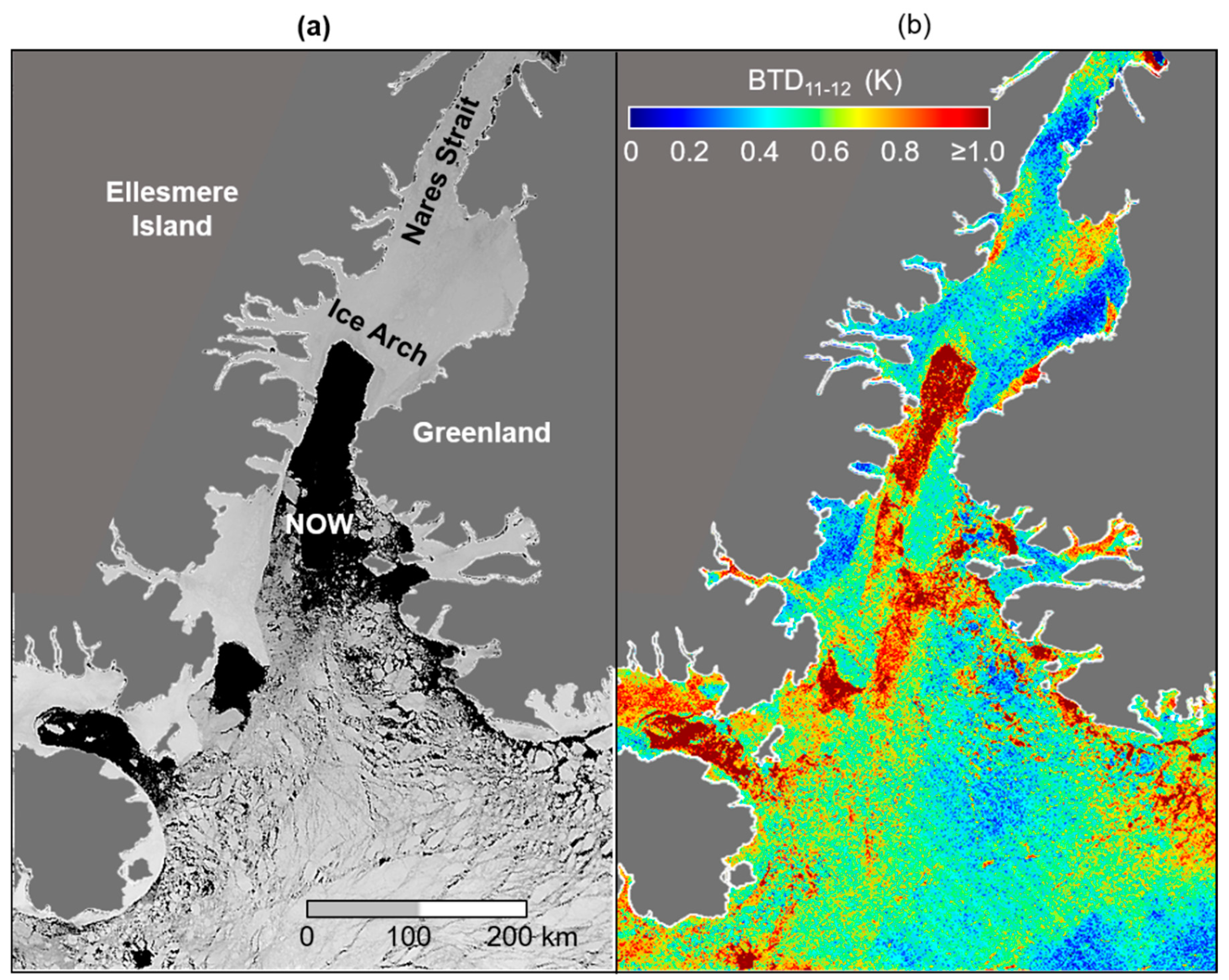
(a) MetOp-A AVHRR image (Channel 1, visible wavelengths) of the NOW for 05 May 2015 with a land mask applied. The NOW is a recurrent polynya that forms when Arctic Ocean floes moving southward through Nares Strait become congested during the colder months and create an ice arch that defines the northern border of the polynya. The ice arch generally breaks down in June or July. (b) BTD11–12 mapping of the same image. There is a large variation in BTD11–12 values, which are generally too high to be attributable to absorption by atmospheric water vapor in the dry Arctic climate.
Figure 2.
(a) MetOp-A AVHRR image (Channel 1, visible wavelengths) of the NOW for 05 May 2015 with a land mask applied. The NOW is a recurrent polynya that forms when Arctic Ocean floes moving southward through Nares Strait become congested during the colder months and create an ice arch that defines the northern border of the polynya. The ice arch generally breaks down in June or July. (b) BTD11–12 mapping of the same image. There is a large variation in BTD11–12 values, which are generally too high to be attributable to absorption by atmospheric water vapor in the dry Arctic climate.

Figure 3.
Vertically pointed emissivity of seawater, snow and ice from 10 μm to 13 μm. BT11 and BT12 channels are indicated for AVHRR and MODIS sensors. (Emissivity values were obtained by averaging datasets available at the MODIS University of California, Santa Barbara Emissivity Library.)
Figure 3.
Vertically pointed emissivity of seawater, snow and ice from 10 μm to 13 μm. BT11 and BT12 channels are indicated for AVHRR and MODIS sensors. (Emissivity values were obtained by averaging datasets available at the MODIS University of California, Santa Barbara Emissivity Library.)

Figure 4.
Emissivity for medium grained snow and bare ice between 10 μm and 13 μm for sensor zenith angles of 0°, 45°, and 60°. (Adapted from Hori et al. [25].)
Figure 4.
Emissivity for medium grained snow and bare ice between 10 μm and 13 μm for sensor zenith angles of 0°, 45°, and 60°. (Adapted from Hori et al. [25].)

Figure 5.
All graphs order CASSTA datapoints by increasing BT11. (a) In situ (M-AERI) and BT11 values have greater divergence for colder temperatures. (b) The difference between in situ and BT11 values increase with greater ice content. Ice pixels have a differential > 2.0 K with an average of 2.4 K, while marginal ice zones and seawater average 1.1 K and 0.4 K, respectively. (c) BTD11–12 is generally associated with colder BT11 owing to atmospheric ice crystals but is not related to the difference between in situ and BT11 values. (d) Sensor zenith angle has no significant relationship to the observed difference between in situ and BT11 values.

Figure 6.
All graphs order the Qaanaaq AVHRR ice datapoints in increasing BT11. (a) In situ (ISAR) and BT11 values. (b) The difference between in situ and BT11 values is similar to the CASSTA datapoints with in situ data > 2.0 K than BT11 and an average of 2.4 K. (c) BTD11–12 values are high and not indicative of atmospheric absorption of water vapor and (d) sensor zenith angle has no significant relationship to difference between in situ and BT11 values, which mirrors the CASSTA dataset.


Table 1.
Characteristics of selected satellite sensors with emphasis on TIR channels utilized for SST and IST retrieval. (AVHRR and MODIS data are used in this study while VIIRS and TIRS are referenced in similar research).
Table 1.
Characteristics of selected satellite sensors with emphasis on TIR channels utilized for SST and IST retrieval. (AVHRR and MODIS data are used in this study while VIIRS and TIRS are referenced in similar research).
| Sensor | Satellite | Total Channels | TIR Channels | TIR Nadir Resolution | Sensor Topology |
|---|---|---|---|---|---|
| AVHRR | TIROS-N, NOAA-6 to NOAA-19 MetOp-A,-B,-C | 6 | Channel 4 10.3 μm–11.3 μm Channel 5 11.5 μm–12.5 μm | 1.1 km | Scanning ±55° 2900 km swath |
| MODIS | Terra Aqua | 36 | Channel 31 10.8 μm–11.3 μm Channel 32 11.8 μm–12.3 μm | 1 km | Scanning ±55° 2330 km swath |
| VIIRS | S-NPP NOAA-20 | 22 | Channel M15 10.26 μm–11.26 μm Channel M16 11.54 μm–12.49 μm | 750 m | Scanning ±56° 3040 km swath |
| TIRS | Landsat-8 | 11 | Channel 10 10.60 μm–11.20 μm Channel 11 11.50 μm–12.51 μm | 100 m | Pushbroom 185 km Swath |
Table 2.
Statistics for the split window and single channel IST when applied to the original CASSTA dataset.
Table 2.
Statistics for the split window and single channel IST when applied to the original CASSTA dataset.
| Algorithm | Ice Regime | Marginal Ice Zone Regime |
|---|---|---|
| Split Window IST | Mean Average Error: 0.144 K Standard Deviation: 0.183 K Average Bias: +0.01 K | Mean Average Error: 0.136 K Standard Deviation: 0.165 Average Bias: −0.03 K |
| Single Channel IST | Mean Average Error: 0.142 K Standard Deviation: 0.182 Average Bias: −0.02 K | Mean Average Error: 0.128 K Standard Deviation: 0.155 K Average Bias: −0.03 K |
Table 3.
Considerations for using CASSTA.
| Consideration | Comment |
|---|---|
| Cloud | Cloud free conditions required. |
| BTD11–12 > 2.0 °C | Indication of ice fog. Inaccurate surface temperature returned. |
| BTD11–12 < 0 °C | Indication of dust. Inaccurate surface temperature returned. |
| Sensor Zenith Angle | Sensor zenith angle <45° for best results. |
© 2019 by the author. Licensee MDPI, Basel, Switzerland. This article is an open access article distributed under the terms and conditions of the Creative Commons Attribution (CC BY) license (http://creativecommons.org/licenses/by/4.0/).
Share and Cite
MDPI and ACS Style
Vincent, R.F. The Case for a Single Channel Composite Arctic Sea Surface Temperature Algorithm. Remote Sens. 2019, 11, 2393. https://doi.org/10.3390/rs11202393
AMA Style
Vincent RF. The Case for a Single Channel Composite Arctic Sea Surface Temperature Algorithm. Remote Sensing. 2019; 11(20):2393. https://doi.org/10.3390/rs11202393
Chicago/Turabian StyleVincent, R.F. 2019. "The Case for a Single Channel Composite Arctic Sea Surface Temperature Algorithm" Remote Sensing 11, no. 20: 2393. https://doi.org/10.3390/rs11202393
Note that from the first issue of 2016, this journal uses article numbers instead of page numbers. See further details here.