A Validation of Fengyun4A Temperature and Humidity Profile Products by Radiosonde Observations

1
School of Atmospheric Sciences, Guangdong Province Key Laboratory for Climate Change and Natural Disaster Studies, Sun Yat-Sen University; Southern Marine Science and Engineering Guangdong Laboratory(Zhuhai), Zhuhai 519082, China
2
Institute of Tropical and Marine Meteorology, China Meteorological Administration, Guangzhou 510080, China
3
College of Environmental Science and Engineering, Donghua University, Songjiang District, Shanghai 20162, China
*
Author to whom correspondence should be addressed.
†
Current address: GuangDong Ocean University South China Sea Institute of Marine Meteorology, Zhanjiang 524088, China.
Remote Sens. 2019, 11(17), 2039; https://doi.org/10.3390/rs11172039
Submission received: 22 July 2019
/
Revised: 23 August 2019
/
Accepted: 24 August 2019
/
Published: 29 August 2019
(This article belongs to the Special Issue Satellite Derived Global Atmosphere Product Validation/Evaluation)
Abstract
:Fengyun4A is the first geostationary satellite with payload of the infrared hyperspectral sounder. The geostationary platform-based instrument can provide observational 3-dimensional fields of temperature and humidity with high scanning frequencies and spatial resolutions. The IR instrument-observed temperature (T) and relative humidity (RH) profiles are closely related to the cloud states. Radiosonde observations are used to validate the Fengyun4A T and RH profiles under different cloud-type sky conditions. The cloud-type information comes from the Himawari-8 satellite which has substantial observing overlap with Fengyun4A over Asia. Taking the radiosonde observation as the reference, Fengyun4A T profile has uncertainty of 2.1 K under clear sky, and 3.7 K under cloudy sky. When cloudy sky is divided into cloud-type skies, the categories have disparities in temperature biases, varying from positive to negative. It is found that most of cloud-type categories have uncertainties of 2.5–3.0 K. The RH profiles have an uncertainty of 18% under clear sky and 21% under cloudy sky in absolute value. On average, the RH biases show neural but positively biased at the dry side and negatively biased at the wet side in the scatter plot. The International Satellite Cloud Climatology Project (ISCCP) cloud type can help to extend the quality flag of the Fengyun4A temperature profile. The impacts from cloud types on IR sounding profiles should be considered in product development or applications.
1. Introduction
The variations of temperature, humidity, and clouds are interwoven in the Earth atmosphere system. Consequently, the observed temperature and humidity profiles have a vast range of applications in atmospheric science studies. Summarized by Yue et al. 2013 [1], the measurements of temperature, humidity, and clouds are used in monitoring climate change [2], evaluating climate models [3], and describing the changes in global circulation, energy, and water cycles [4]. The Geostationary satellite-based infrared hyperspectral sounder has higher scanning frequency than the polar orbit satellite-based sounder. The high scanning frequency can enhance the applications of the observed temperature (T) and relative humidity (RH) profiles, especially in severe weather descriptions and predictions. The T and RH profiles have evident and fast changes during the developing and decay processes of the small and mesoscale weather system [5]. The frequent and continuous observations on the 3-dimensional structure of temperature and humidity provide a chance to monitor the environments, which can generate or develop the weather systems. So far, the infrared hyperspectral sounder on the Fengyun4A (FY4A for short) satellite is the only instrument that can provide this kind of service [6].
Except for IR bands, microwave bands are also used to sound the T and RH profiles. The microwave sounding system can penetrate clouds but usually has limited channels due to the flat shape of weighting functions. For example, the Microwave Sounding Unit (MSU) has only four channels. The Advanced Microwave Sounding Unit (AMSU) has 20-channels. The conceptual hyperspectral microwave atmospheric sounding proposed by Blackwell [7] has about 100 channels, which are far less than that of IR soundings such as Infrared Atmospheric Sounding Interferometer (IASI) and Atmospheric Infrared Sounder (AIRS). IASI has 8461 channels with spatial resolution of 12 km and AIRS has 2378 channels with spatial resolution of 14 km [8]. Both IASI and AIRS have high vertical resolution: 101 layers for the range from sea surface to 1 hPa. However, the T and RH profiles measured by IR sounders are interfered with by the clouds. Previous studies on the polar satellite-based IR sounders show that the cloud states are highly related to the data quality of T and RH profiles [1,9]. Studying the IR sounding under cloudy conditions can benefit the high vertical resolution and all-weather applications.
As the first geostationary satellite with hyperspectral IR sounder, the FY4A satellite was launched on 11 December 2016. The primary payloads of FY4A are the Advanced Geosynchronous Radiation Imager (AGRI), Geostationary Interferometric Infrared Sounder (GIIRS), and the Lightning Mapping Imager (LMI). The AGRI has 14 spectral bands with spatial resolution of 0.5 km and scanning frequency of 15 min. GIIRS can provide the vertical temperature and humidity profiles at 101 levels from the surface to 1 hPa. There are two observation modes for the GIIRS: the whole China area mode and mesoscale mode. The GIIRS has hourly observation frequency with surface horizontal resolution of ten kilometers under the full China area mode.
The LMI can observe the lighting activity, which is a useful indicator of deep convection events. The common platform of these three instruments provides a chance to study the developing process of convection systems and extreme weather events. The observation of atmospheric vertical structure with features of high resolution, broad coverage, and high renew frequency provides the ability to estimate the atmospheric stability indexes such as the Convective Available Potential Energy (CAPE) for mesoscale weather systems. The atmospheric stability indexes calculated from the IASI and AIRS sounding products show 1–6 h before the convection development [10]. The accuracy of temperature profile is of vital importance in such an application. The GIIRS has similar spectral coverage to that of AIRS and IASI. Based on the radiances from 1650 channels, GIIRS can provide temperature profile, water vapour profile, and ozone profile. The spectral ranges of GIIRS are 8.85–14.29 m and 4.44–6.06 m [6]. The retrieval of temperature profile is based on the several hundred channels on the band of 8.85–14.29 m. Band 4.44–6.06 m is used to retrieve the humidity profile. The absorption and emission materials are carbon dioxide (CO) and ice particles at the band 8.85–14.29 m. IR sounder at this spectral range can be used to measure temperature and humidity profile because of the absorption by CO and water. The existence of clouds interfere with the retrieval of temperature and humidity profiles through absorbing and emitting IR radiances. The net radiative effects of clouds on IR bands vary with cloud type [11]. Clouds on the light path may attenuate IR radiance for the below-column CO emission. The emission from clouds may enhance the IR radiance, which relates to the temperature at the above column of the cloud layer. Clouds have huge variation in vertical geometry range, from the surface to tropopause. Correspondingly, clouds may have impacts to the retrieval of T and RH over a sizeable vertical range. The retrieval of T and RH profiles under cloudy sky conditions is still a great challenge. The IASI provide operational T and RH profile products under clear sky and cloudy sky but based on different algorithms [12].
Validation in the performance of IR sounding measurements under cloudy sky is an essential pre-step of the applications. The ground-based radiosonde measurements are used as the reference to do the validation. The data are from 120 L-band radar radiosonde sites in China. Through the comparative observation, those L-band radiosonde instruments have similar accuracy to Vaisala RS80 radiosonde [13]. The Vaisala RS80 radiosonde has height-dependent uncertainties: 0.4 K in the vertical range from surface to 100 hPa, 0.6 K in the range of 100 to 20 hPa and 0.8 K above 20 hPa [14]. Compared with microwave radiometer measurements, RS80 has about 5% dry bias in the humidity [15]. The RS80 measured RH has dry bias throughout the troposphere. The bias becomes evident when temperature is lower than −20 C [16]. Compared with reanalysis and observations by the GPS radio occulation, the L-band radiosonde temperature shows bias of 1–2 K and the RH shows dry biases [17].
Cloud coverage varies from different climate zones but has a global average of 75% based on the active sensor [18] and about 70% based on the passive sensor [19]. For the area focused on in this study, the average cloud fraction is about 61% over China region [20]. Cloud properties such as phase, height, and optical depth also impact the IR sounding retrieval. Optically thick clouds can totally attenuate the below signal. Some thin clouds are difficult to detect by passive sensors [21]. Clouds introduce errors to the first generation of IR soundings, such as TIROS (Television Infrared Observation Satellite Program), Operational Vertical Sounder (TOVS), and ATOVS (Advanced TOVS) [22,23]. Physically-based radiative transfer models such as DISORT [24] are used to estimate the cloud radiative property at IR band so that the hyperspectral IR soundings can gather radiances data to estimate profiles under partial cloudy sky [25,26]. Cloud status changes very fast during the development and decay processes of weather systems. The assessments of the impacts from different types of clouds on the IR sounding products will be necessary for the application in weather.
Clouds are efficient emitter/absorbers at IR bands [27]. The cloud may induce errors and uncertainties to the IR sounder measured T and RH profiles [28]. According to the study on AIRS, the impacts from clouds may be different between cloud categories [1,9]. The extensive and uniform stratus dominates the uncertainty of stability derived from AIRS [1]. The data quality is related to the cloud type and surface condition. The AIRS temperature retrieval yields more than 90% of good quality cases under clear sky and 50% to 80% under shallow convective but less than 10% for optically thick clouds [9].
Following the methods used by Yue et al. 2013 [1], ISCCP (International Satellite Cloud Climatology Project) cloud-type products are used in this manuscript to classify the cloud impacts. The ISCCP classified cloudy scenes into 9 cloud types according to cloud-top pressure and cloud optical thickness [29]. ISCCP collects radiances from 8 geostationary weather satellites (including Himawari-8) to clarify the coverage and variation of clouds [30]. The visible (VIS) and IR radiances from satellite imagers are calibrated. The calibrated radiances are converted to optical depth and cloud-top pressure. A cluster analysis is applied on the cloud optical depth and cloud-top pressure to produce the cloud-type product [31,32]. Cloud microphysical properties determine the radiative effects of clouds, which are spectrally varying. Conversion of satellite-measured radiance to the cloud properties is a fundamental but complex step in the field of remote sensing. ISCCP provides a relatively uniform cloud product over the low and middle latitudes but can also have enough time and space resolution [33]. The ISCCP cloud product has been extensively applied in characterizing the cloud effects in climate. The temperature and humidity profiles from the GIIRS are basically from the IR channels. Clouds interfere in retrieving profiles through absorption on the path and the emission from the below clouds. In other words, cloud interference is related to the radiative properties and geometry properties. Cloud classification according to the definition of ISCCP cloud-type product is expected to help to reduce the uncertainty of IR sounding profiles.
Three independent datasets are used in the study: the temperature and humidity profiles of GIIRS onboard of FY4A, the ground-based radiosonde data and Himawari-8 cloud-type product, which contains the ISCCP cloud-type variable. Radiosonde observation is used to validate the performance of GIIRS under the clear sky and ISCCP cloud-type skies.
2. Data and Method
The FY4A program has generated profile data since January 2018 but the data are only publicly available from May 2018. The dataset contains the temperature profile, humidity profile, and ozone profile from surface to 1 hPa with 101 levels. The observation has 16 km by 16 km resolution at surface and hourly scanning frequency. The swath of the sensor is about 250 km aside from the scan line and about 500 km in total. The data are available at the Chinese National Satellite Meteorological Center (NSMC, http://satellite.nsmc.org.cn/PortalSite/Data/Satellite.aspx).
The radiosonde data are used to validate the FY4A T and RH profiles. The sounding balloon was released twice a day: 8 a.m. and 8 p.m. Beijing time (UTC+8). In this study, we use sounding observation of 120 sites around China to the survey. The sounding measurement can provide T and RH profiles with resolution in several meters.
The ISCCP cloud-type information is from the Himawari-8 observation. The Himawari-8 cloud property product has a spatial resolution of 5 km and a temporal resolution of 10 min. The dataset contains ISCCP defined cloud type, cloud optical thickness, cloud effective radius, cloud-top temperature, and other cloud information but is only available during daytime. The Japan Meteorological Agency (JMA) has served the ISCCP program since 1983. The new Japanese generation of geostationary satellites can provide a stable source for the ISCCP cloud type [30]. More information about the new ISCCP dataset has been discussed by Young et al. 2018 [34].
For validation, referenced observation must be from an independent platform. The different systems have their own errors in different principles [35]. The radiosonde and GIIRS have different vertical and horizontal scales in observation. In other words, the observations from independent platforms have non-coincidence error. To solve this kind of non-coincidence problem, Pougatchev et al. [36] used a mathematical correlative method to validate the IASI profiles by the radiosonde observation in site. Divakarla et al. [37] validated the AIRS by the radiosonde data by collocating the data into a 100 km radius and ±3 h of the radiosonde observation.
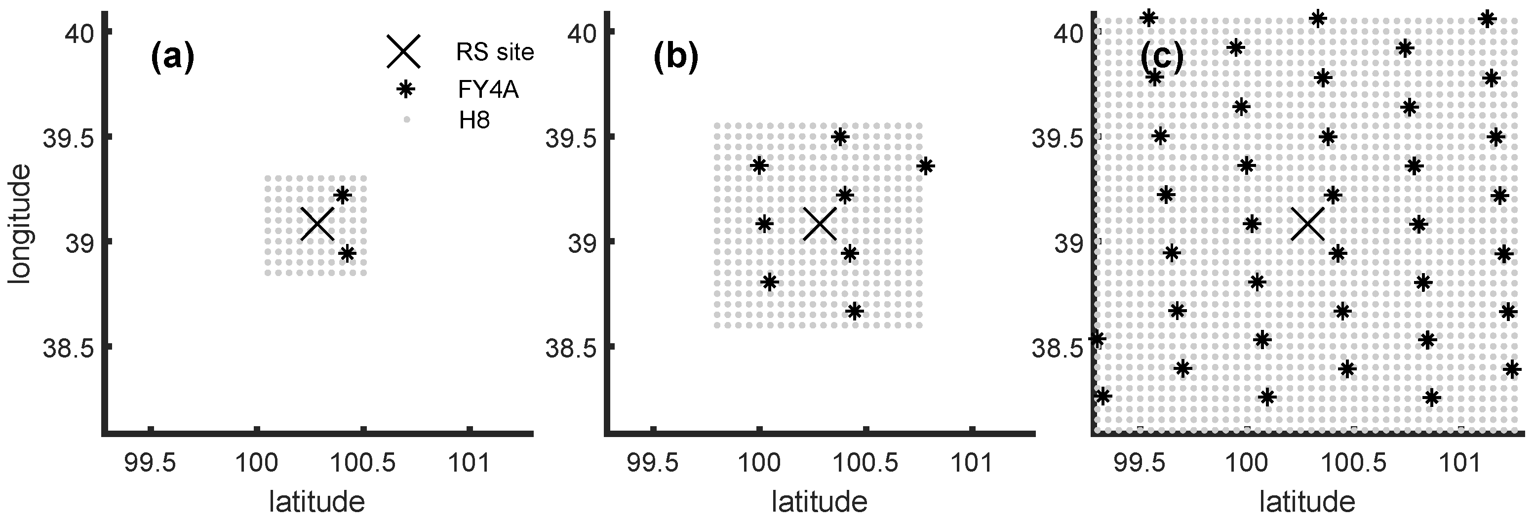
FY4A locates at the 104.7E in longitude of the geostationary Earth orbit, while the Himawari-8 locates at 140E. The observational disks of both satellites have large superposition area in China. Thus, we collocated the FY4A data, Himawari-8 data and radiosonde data together in time and space. The sounding balloon drifts following the atmospheric motion during the process of rising. On average, it is about one hour for the sounding balloon to the end of rising (balloon burst) since the release. The drifting distance depends on the horizontal wind speed. After one hour of drift, the balloon travels about 50 km in horizontal distance from the location of release. We assume that the radiosonde observation represents the atmospheric status at the average scale of one hour and 50 km. FY4A data and Himawari-8 data are collocated to the location of sites and the time of balloon releases. To match the scale of radiosonde measurement, we use the average over one hour after the release. The collocation of 3 platforms is shown in the Figure 1. Under the rules of collocation, there are 42,208 valid profiles screened out over the investigated period: from January 2018 to November 2018.
After data collocation, the physically unreasonable cases are discarded: temperature which exceeds the range of −100 C to 50 C and RH which is out of range from 0 to 100%. Supposing the radiosonde data represents the real value of the T and RH profiles, the difference between the FY4A temperature and radiosonde temperature is used to stand for the bias and the standard deviation (or RMS) to represent the uncertainty.
3. Results
3.1. Fengyun4A Data Quality Flags
The data quality of FY4A temperature and humidity profile products is suggested with a quality flag by the Fengyun science team. The data qualities are categorized into four types: (1) perfect, (2) good, (3) bad, and (4) very bad or do not use. The quality flags are relevant to each vertical point of every profile. Around the time of balloon release (8 a.m. and 8 p.m. local time) and the location of radiosonde sites, about 1.48 million FY4A profiles are collected in total. Since the existence of clouds can interfere the IR signal directly, the distributions of temperature and humidity qualities are examined over clear and cloudy sky separately.
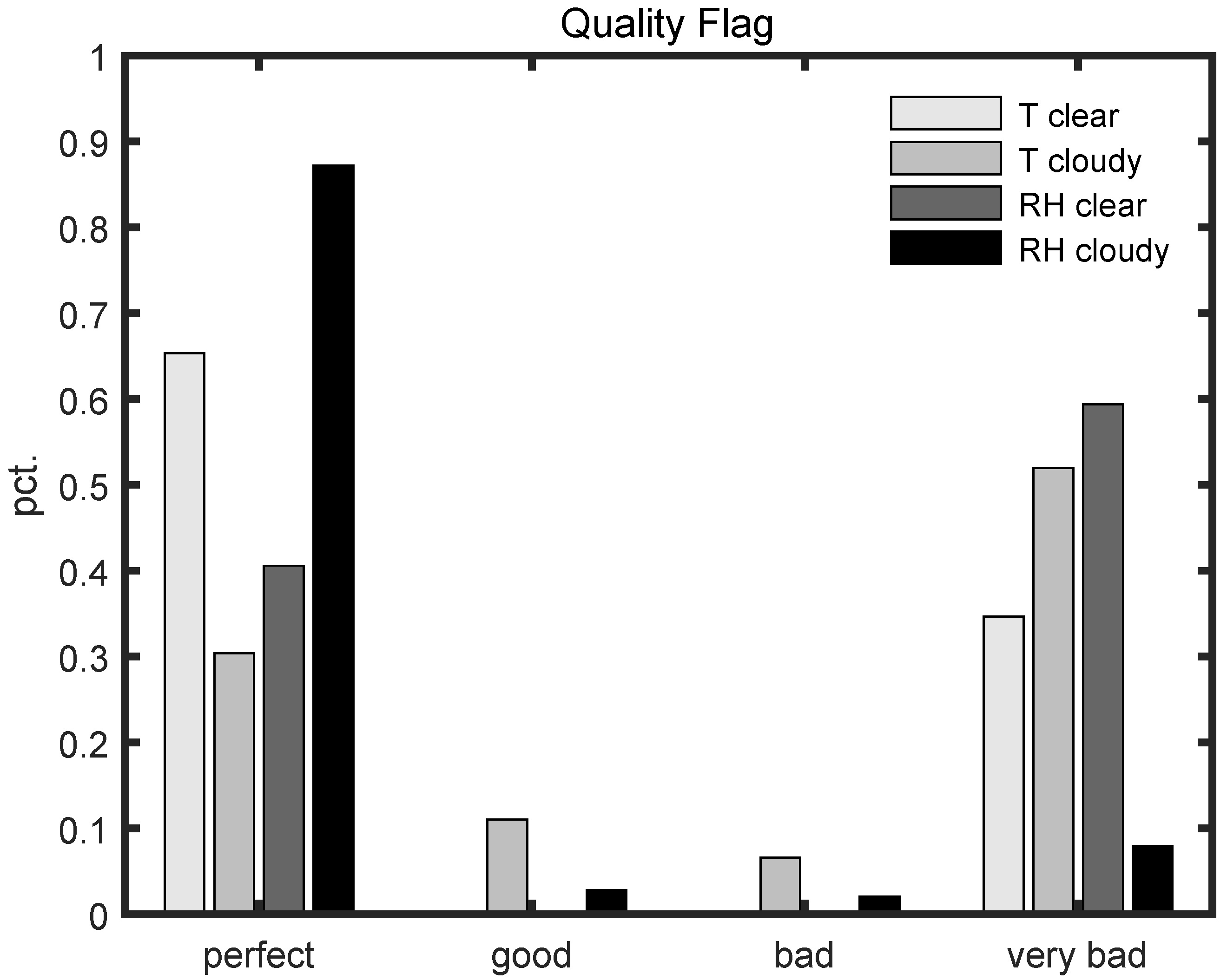
Figure 2 shows the distribution of FY4A data quality flags under the clear sky and cloudy sky. Under the clear sky, the data only has categories of “perfect” and “very bad”. 65% of temperature observations under clear sky are categorized as “perfect”. But the percentage decreases to about 33% under the cloudy sky. 35% of temperature observations under clear sky are categorized as “very bad” and the percentage increases to 50% under the cloudy sky.
The quality of humidity shows different behavior on the percentages under the clear sky and cloudy sky. 41% of RH cases are labeled perfect under clear and 89% under cloudy. Only 6% of RH cases are categorized into “very bad” under the cloudy sky, but 60% of RH cases are in the class of “very bad” under the clear sky.
The temperature has more perfect cases under clear sky than that under the cloudy sky. The humidity has fewer perfect cases under clear sky than that under the cloudy sky. The distribution of temperature quality is as expected, but the humidity is not since there is a higher perfect percentage at cloudy than under clear.
3.2. Validation of Temperature
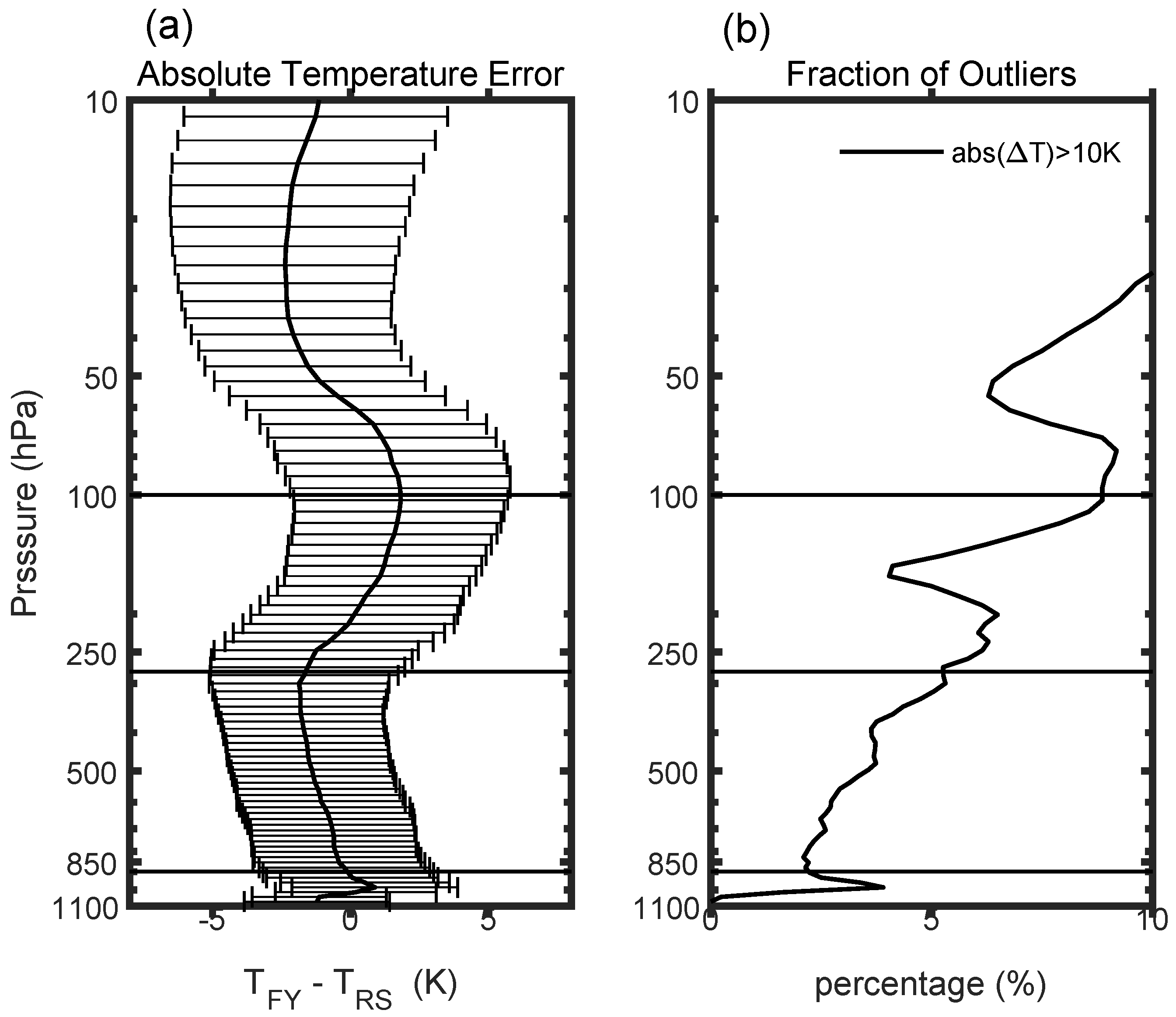
Determined by the weighting functions, the IR sounder profiles the temperature from the absorbing differences on the channels. The uncertainty of the temperature may be altitude-dependent because of hardware sensitivity and some other factors. The designed uncertainty (RMS) of the FY4A temperature is about 0.8 K between the 300–700 hPa and about 1.6 K above the 250 hPa [38]. According to the vertical distribution of biases and the meaning in the meteorological conventions, the vertical layers are partitioned into 4 parts (see Figure 3). PBL (Planet Boundary Layer): from the surface to the 900 hPa, this layer has the contamination from the surface emission and represents for the planetary boundary layer, the mean bias has irregularly variation with height, and the signal may have contamination from the surface. TL (Troposphere Layer): the layer from 900 hPa to 300 hPa, this layer represents the Troposphere Layer(TL). TPL (TropoPause Layer): the layer from 300 hPa to 100 hPa, this layer represents the Tropopause Layer (TPL). Through the definition of turn points of the temperature deviation, most of the profiles have tropopause in this vertical range. SL (Stratosphere Layer): the layer from 100 hPa to 10 hPa, this layer represents the Stratosphere Layer (SL). These definitions are different from the traditional conventions in meteorology. These partitioned layers are used to represent the PBL, TL, TPL, and SL. The upper limit is set at 10 hPa because very few radiosonde balloons can exceed 10 hPa.
The percentages of the outliers are shown in the Figure 3. The cases with the FY4A temperature and radiosonde temperature difference larger than 10 K are defined as outliers. The fractions of outliers increase with height. At the PBL and TL layers, the outlier percentages are smaller than 5% with local minimum at the TPL. The outlier percentage exceeds 10% in the SL.
The FY4A team provides the QC flags to the temperature and humidity profiles. All profiles have QC (quality control) label at all the 101 vertical bins. We validated the FY4A products for the good and bad cases separately. For the “good” cases, the main purpose is to validate the FY4A by providing the statistical properties of the new observation. For the “bad” cases, the primary purpose is to show the impacts of the clouds on the data quality.
3.2.1. Validation of Temperature with QC Flag of “Good”
According to the collected data ensemble, the temperature has 65% of perfect cases under the clear sky and 33% of perfect cases under the cloudy sky (Figure 2). The cases with QC flags of perfect or good are used in this part of study.
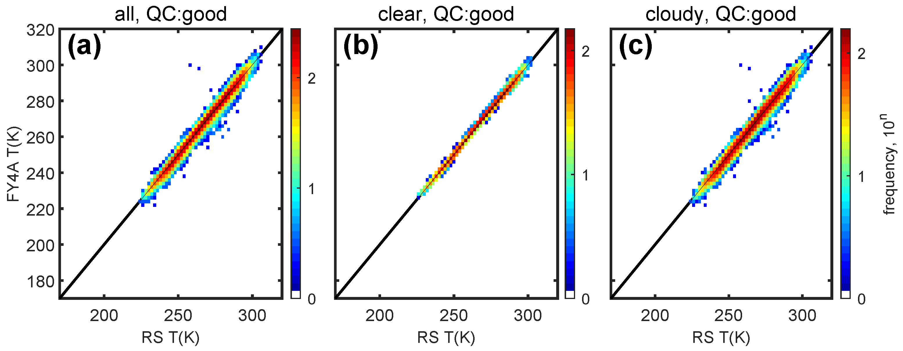
First, the 2D-histogram plots of the all-sky, clear sky and cloudy sky are shown in the Figure 4. The plots include the vertical range from 10 hPa to the surface. Most of the cases are in the range of 200 K to 320 K. FY4A temperature has an average bias of −0.3 K and uncertainty (RMS) of 3.0 K for the all-sky condition. The biases under clear sky and cloudy sky are −0.2 K and −0.4 K respectively. The uncertainties under the clear sky and cloudy sky are 2.1 K and 3.7 K, respectively. The biases between the clear-sky sub-ensemble and cloudy sky sub-ensemble are close to each other. The clouds have evident impacts on uncertainty: the uncertainty of the cloudy sky sub-ensemble is almost twice that of the clear-sky sub-ensemble. The uncertainty of temperature lower than 230 K is bigger than the uncertainty of temperature higher than 230 K. This phenomenon is consistent with the designed goal: the uncertainty is bigger at the stratosphere than at the troposphere [38].
The temperature uncertainty is dependent on clouds and height. The ISCCP cloud-type classification is used to verify the impacts from different cloud types on the temperature uncertainty. During the data collocation, the Himawari-8 data are collocated to the radiosonde data at the site locations and the times of balloon release. In the collocation time and space intervals (one hour after releasing and 0.5 separately), Himawari-8 may scan the target area many times. The sky conditions may vary with time and space intervals according to the ISCCP cloud type. We use the most frequent cloud type to label the sky condition for each profile. In order to reduce the interlaced cloud type, the standard deviation of the cloud type has a restriction on the up limit of 1.2.
The 2D histogram plots of the sub-ensembles with 10 ISCCP cloud types are shown in the Figure 5. The vertical range from 10 hPa to the surface is included in the plots. The statistical properties of the sub-ensembles which are with different ISCCP cloud types and at the different layers are shown in Table 1. Over the sub-ensembles with different cloud types and layers in height, the biases and uncertainties show averages of −0.3 K and 0.8 K respectively. The average bias is equivalent to the value of the bias of the whole ensemble, which includes both clear and cloudy cases and vertical range from 10 hPa to the surface (Figure 4a). The biases of sub-ensembles vary from each other. Under some cloud types, the uncertainties are equivalent to or even smaller than the clear-sky uncertainties. However, others have evident larger uncertainty than that under the clear sky. Most of the sub-ensembles with ISCCP cloud-type labels are smaller than the uncertainty of cloudy sky in total (3.7 K) which is shown in the Figure 4c.
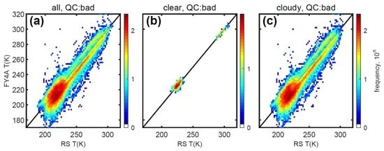
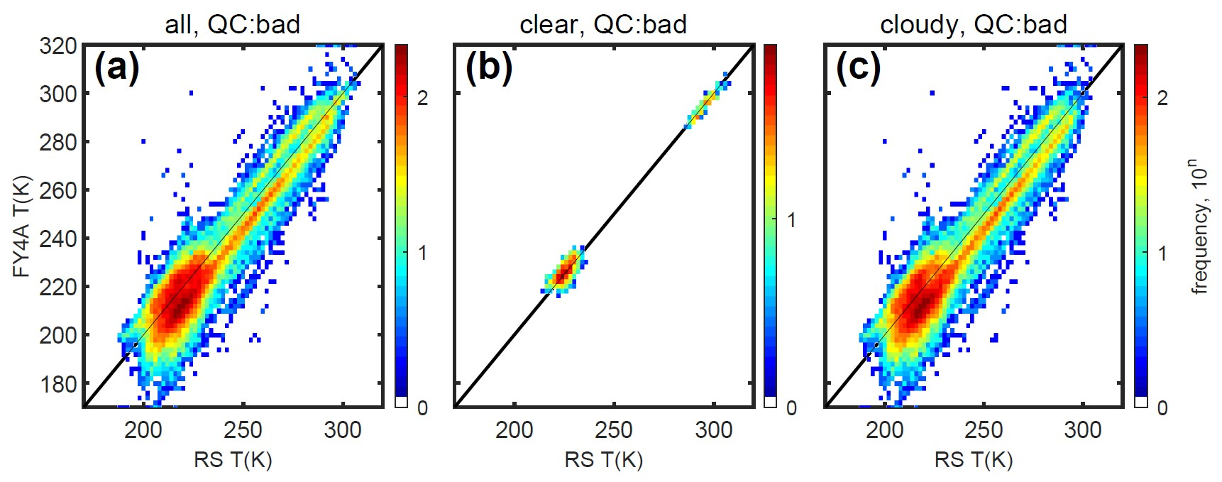
3.2.2. Validation of the Temperature with QC Flag of “Bad”
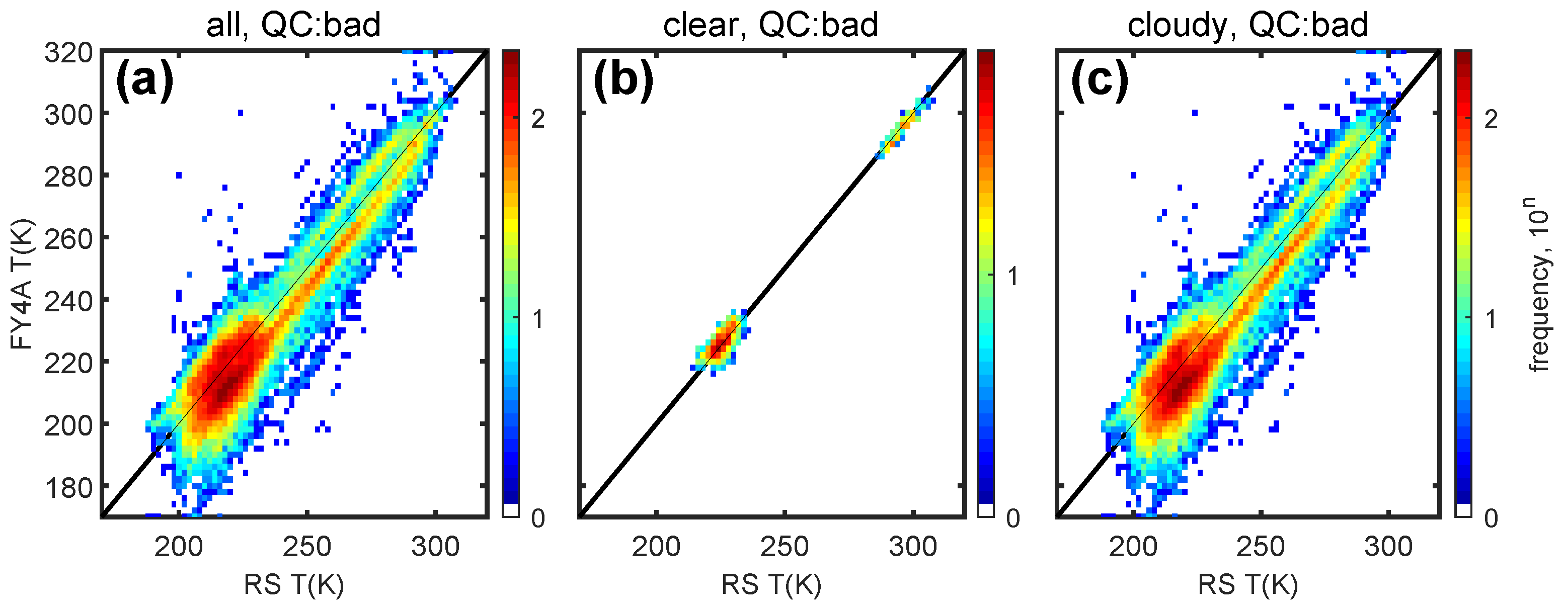
This section focused on FY4A temperature cases with “bad” or “very bad” quality flags. 33% of temperature cases are categorized into “very bad” under the clear sky, and about 50% are “very bad” flagged under the cloudy sky. The 2D-histogram plots of FY4A temperature which are with “bad”-quality flags and the radiosonde measurements on temperature are shown in Figure 6. The ensemble of total cases which includes both clear sky and the cloudy sky has the bias of −3.5 K and uncertainty of 10.0 K. The sub-ensembles of clear sky and cloudy sky have biases −0.9 K and −3.8 K, respectively. The uncertainties under clear and cloudy are 4.0 K and 10.4 K, respectively. The uncertainty under cloudy is 2.6 times the uncertainty under clear.
Under clear sky, the ”bad” flagged cases only exist at temperature colder than 230 K or warmer than 260 K. For the typical temperature profile, 230 K locates at the height of the tropopause. The 270 K and higher locate at the layer of near-surface or PBL. Although the data are with the quality label of “bad”, the sub-ensemble at the clear sky has the uncertainty of 4.4 K at the layer above the tropopause and 2.1 K at the layer close to the surface. This uncertainty is at the same level of the “good” quality ensembles.
Uncertainties of the “bad” flagged sub-ensembles show huge differences between the clear sky and cloudy sky. The average uncertainty of the cloudy sub-ensemble is 10.4 K. From the scattering plots, the FY4A temperature has two distinct behaviors when the temperature is higher or lower than 240 K. At the cold side, which means the temperature is lower than 240 K and the vertical equivalence location are tropopause and above, the scattering elements are continuously centered around the identity line. At the warm side, the scattering elements are distributed around two identity-line paralleled lines. Most of the cases are around the line and below the identity line, and the second line is above the one-by-one line. This phenomenon means one group case is underestimated and the other group case is overestimated.
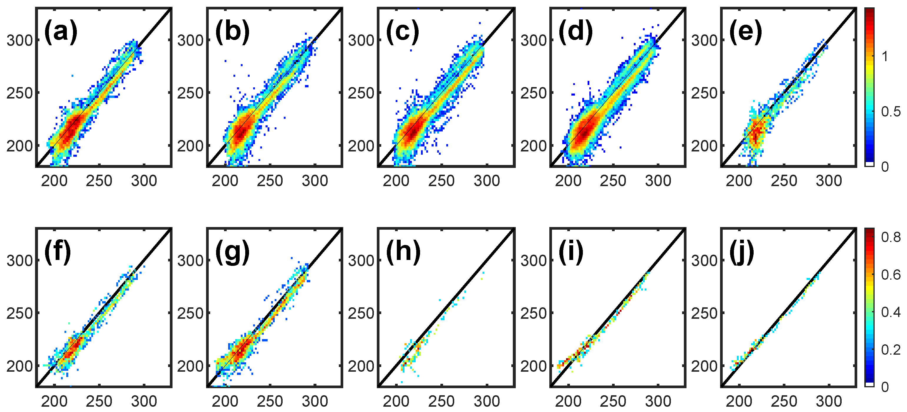
To verify the impacts from the different types of clouds, the histogram plots on radiosonde and FY4A T profiles with ISCCP cloud-type categories are shown in Figure 7. All the sub-figure covers the vertical range from 10 hPa to the surface. The statistical properties of the sub-ensembles, and further divisions on height layers, are shown in Table 2. The case numbers, mean biases and uncertainties (RMS) are given in the table for the sub-ensemble with different layers and ISCCP cloud type. The height layers are labeled with ST, TPL, TL, and PBL. Both biases and uncertainties show apparent disparities between the sub-ensembles.
For the whole cloudy ensemble, the bias is −3.8 K and the uncertainty is 10.4 K. In general, the biases are negative among the categories with cloud-type and height. The biases also show diversity between the sub-ensembles. The stratus cloud sub-ensembles have positive bias, and the other types of clouds have negative biases which varies from −2 K to −5 K. The uncertainties among the sub-ensembles also show evident diversity. The uncertainties have an average of 10.4 K under the cloudy sky and with minima of 3.4 K under the stratus cloud and maximum of 12.2 K under the nimbostratus cloud.
The phenomenon of the scatter plot of FY4A and radiosonde temperature centering around two lines under the cloudy sky Figure 6c is evident under some types of cloud but not on the others. The most evident is under the cloud type of deep convection. The deep convection usually has considerable optical depth and geometry depth enough to remove the signal from the inner part of the cloud system. The cirrus and cirrostratus clouds also show weak positive centering line which is above the identity line. Some scattering elements are above the one-by-one line but without the centering line under the cloud type of altocumulus, altostratus, and nimbostratus. Scatter elements are above the identity line and the positively biased centerline did not show up under cloud of cumulus, stratocumulus, and status. The uncertainties under the cumulus, stratocumulus, and stratus are relatively small: 9.5 K, 5.4 K, and 3.4 K. However, the case numbers of some sub-ensembles are on the order of hundred or even less. More cases are necessary to increase significance.
3.3. Validation of Humidity
Water content and its variation at stratosphere layer and above are negligibly small, relative to that at the troposphere. For the RH part, we focus on the layer from the surface to 280 hPa (about 10 km). The FY4A team also provides quality flags to the humidity product. About 40% of humidity cases are with the flag of “perfect” under the clear sky, but over 90% cases are with the flag of “perfect” under the cloudy sky (Figure 2). For the “bad” or “very bad” flagged cases, we did not find a good coincidence between the FY4A humidity and radiosonde humidity. In this part of the study, only the “perfect” or “good” flagged RH cases were considered. According to the results shown below, the RH uncertainty is larger than the designed target.
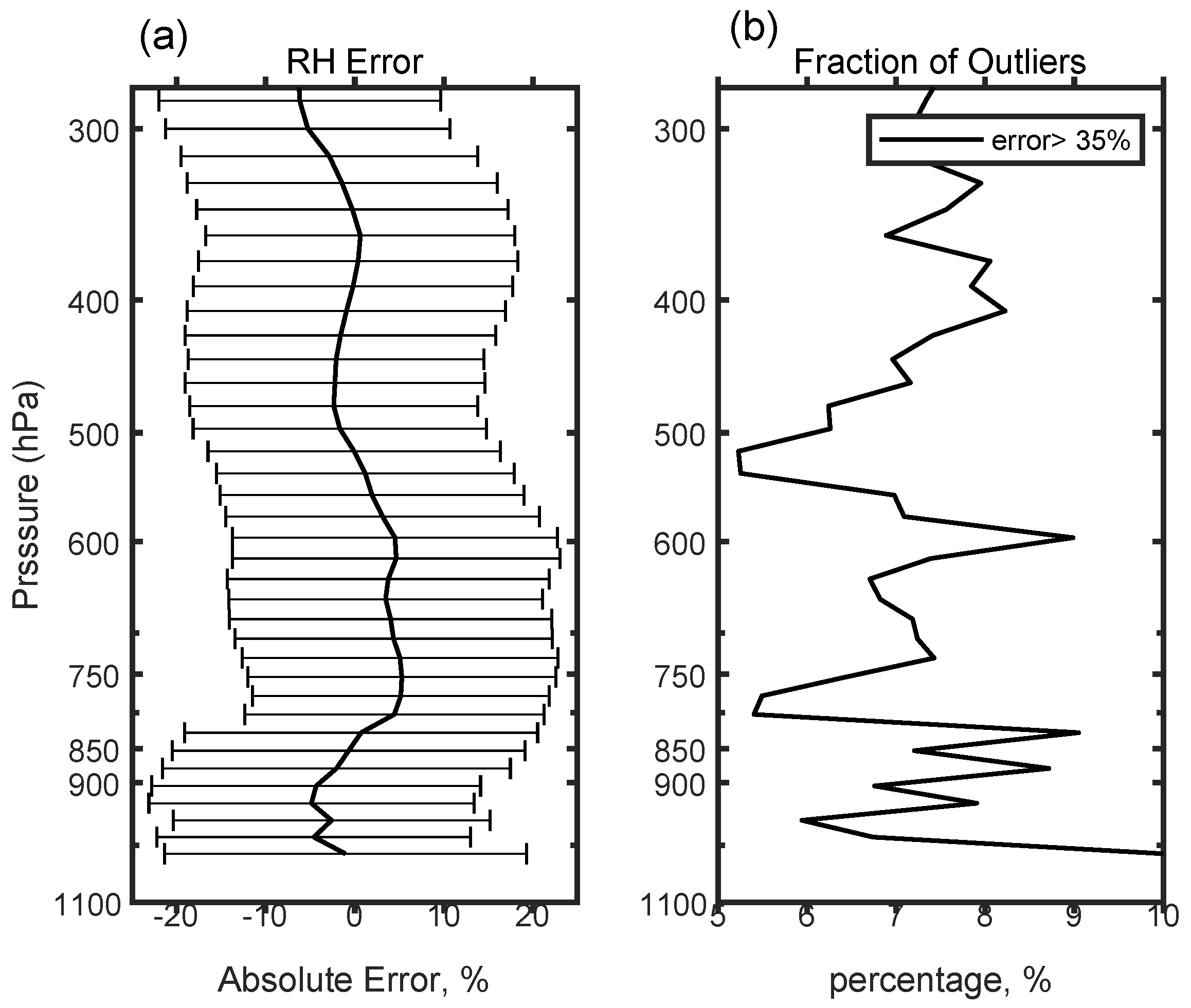
From Figure 8a, the averaged RH bias is neutral at about 0.1% but shows variation with height. The biases fluctuate from -5% to 5% below 500 hPa. The RH biases tend to be negative from 500 hPa to 280 hPa, which means FY4A humidity is overestimated. The averaged uncertainty is 21% and varies in the range from 18% to 25% with height. The Figure 8b shows the percentage of outlier. The outlier is defined by the bias larger than 35% which is about two times of the RH std under clear-sky condition. Averaged over the layer from the surface to 280 hPa, about 7% of cases are outliers. The outlier percentage fluctuates within the range from 5% to 10% below 500 hPa and remains a constant above 500 hPa.
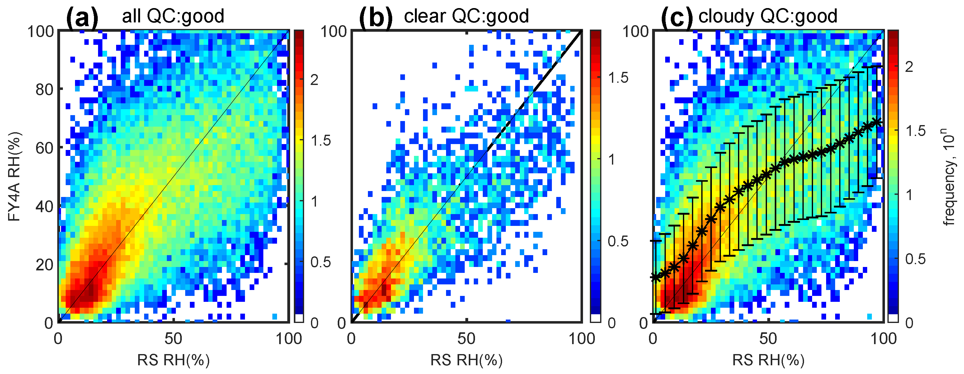
Figure 9 shows the 2D-histogram plots of the radiosonde RH and FY4A RH. For the sub-ensemble of all-sky, the bias is 0.5% and uncertainty is 20% in the absolute unit (we use absolute value for the RH except for special declaration). Most of the cases are in the RH range from 0 to 50%. In the range from 50% to 100%, FY4A humidity has negative biases which means the FY4A humidity is underestimated.
Under clear sky, shown in Figure 9b, both radiosonde and FY4A show few occurrences of saturation. The sub-ensemble has bias of −0.9% and uncertainty of 18%. The designed goal is 5–10% in the layer of the troposphere [38]. The observed RH uncertainty is slightly higher than the designation under clear sky.
The existence of clouds has evident impacts on the retrieval of the humidity profile. The validation on cloudy cases is shown in the Figure 9c. The cloudy sub-ensemble has the bias of −1% and uncertainty of 21%. The FY4A humidity has different biases at the dry side and wet side of the scatter plot. The FY4A humidity is overestimated when the RH is less than about 40% and underestimated when RH is greater than 65%. The biases and the uncertainties are represented by the error bar plot in the figure.
As a similar consideration, the impacts from cloud type on the humidity are separated according to the Himawari-8 cloud type products. Figure 10 shows the 2-dimensional histogram distribution of FY4A humidity and radiosonde humidity. The sub-ensembles with different ISCCP cloud-type conditions are shown in the sub-figures. The corresponding statistical properties are shown in Table 3. The biases of RH do not show an evident difference between the sub-ensembles. Only sub-ensemble with altocumulus has a bias of 4%. The other cloud-type sub-ensembles have biases of 1% to 2%, which means the FY4A humidity is slightly overestimated under the condition of the cloudy sky. The sub-ensembles of cumulus, stratocumulus, and stratus have limited sample numbers: in the order of hundreds. The uncertainties of the sub-ensembles are from 19% to 21%. These values are similar to that of the cloudy ensemble. The uncertainties of the cloud-type sub-ensembles do not show evident differences from each other. The sub-ensembles of cirrus, cirrostratus and deep convection have similar biases trend shows in the Figure 9c.
4. Discussion and Conclusions
The ground-based radiosonde observations are used to validate the data quality of atmospheric profile product of the newly launched geostationary meteorological satellite FY4A. The payload of GIIRS works at the IR spectral range of 8.85–14.29 m and 4.44–6.06 m. Clouds show significant impact on the IR spectral sounding products when the cloudy and clear cases are compared. In order to assess the impacts by the clouds, the Himawari-8 ISCCP cloud type was collocated with the FY4A and radiosonde observations. The statistical properties of FY4A profiles show disparity among the ISCCP defined cloud-type categories. In principle, the ISCCP cloud product originates with the spectrally distributed radiances over the visible and infrared channels.
According to the spectral differences in radiances, after the processes of radiation calibration, radiative transfer model comparison and statistical analysis, the clouds are divided into nine types. In reverse, the ISCCP cloud classification classifies the cloud-resulted spectral differences in IR radiance. As an efficient IR emitter, the clouds contribute to the radiances as its emission and/or attenuation. Because the clouds contain large particles, scattering effects should be considered which are usually ignored in the sounding algorithm [39,40]. The contribution from clouds to the sounding radiances is substantially evident. Different ISCCP type of clouds has its own spectral character in IR bands. Thus, the sub-category on the cloudy sky into cloud type sky is necessary for the IR sounding system.
Three points are raised in the comparison among the 10 types of sky conditions (nine types of clouds plus clear sky). The temperature shows most significant biases when the sky is low clouds overcast such as the cumulus and stratocumulus. Cumulus and stratocumulus can impact the biases at troposphere and stratosphere. The sub-ensemble of deep convection has smaller temperature biases (about 0.5 K) than expected. The sub-ensemble of cirrus or cirrostratus has small biases (about 0.5 K) but huge uncertainties(3 K).
The cumulus and stratocumulus usually cover a large area which may exceed the collocation scale. The optically thick clouds play as the pseudo-surface. The improper estimation in cloud heights and so on may change the shape of weighting functions and result in systematic errors. The deep convection system may be smaller than 50 km. There is some possibility that the collocation zone is half occupied by deep convection system. Meanwhile, a deep convection system has large enough optical depth that it removes the IR signal from lower layers. The statistical values for the sub-ensemble of deep convection may come from other types of sky conditions. The cirrus clouds have huge variations in orientation, particle size and shape, height, and so on. Sometimes, passive sensors have difficulty in detecting the thin ice clouds. The uncertainties in the cirrus clouds propagate to the uncertainties of temperature through the alternation of weighting functions.
Observations from three independent platforms are collocated into the same time and location. The basic idea is that the balloon sounding takes about 1 h to finish the rising processes, and the balloon drifts less than 50 km in horizontal distance within the time of rising. The FY4A and in-site radiosonde are collocated with the time interval of 1 h after the releasing of the balloon and with space distance of 0.5 in latitude and longitude. This time and space interval is selected to coincidence with the balloon rising process. Himawari-8 data is collocated into the ensemble with the same rules. Himawari-8 and FY4A can scan the radiosonde site several times during the collocation time interval. The clouds keep changing during the collocation time. We did not consider the changing cloud mask but use the most frequent cloud mask index instead.
The ratios of “good” case numbers and “bad” case numbers have evident differences between the clear sky and cloudy sky conditions. The existence of clouds can impact the data quality at the current data processing system. For the temperature profile, the sub-ensemble of “good” flagged FY4A cases and sub-ensemble of “bad” flagged FY4A cases are analyzed separately.
For the temperature ensemble with “good”-quality flags, the ensemble has the bias of −0.3 K and uncertainty of 3.0 K under the all-sky condition. The sub-ensembles of clear sky and cloudy sky have close biases. The uncertainties show evident difference between the clear sky and cloudy sky. The clear sky has the uncertainty of 2 K which is close to the designed target, but the cloudy sky has the uncertainty of 3.7 K, almost double that of the clear sky. When the cloudy sky is divided into sub-ensembles according to the ISCCP cloud type, both biases and uncertainties show disparities between the sub-ensembles. The biases vary from negative to positive. Most of the changing magnitudes are within 1 K. Uncertainties reduced from 3.7 K to about 2.5 K through the division of cloudy sky into cloud type sky. Some sub-ensembles such as cirrostratus and stratocumulus have uncertainties larger than that of the cloudy sky. The classification of cloud type can help to source the error and enhance the applications of IR spectral sounding.
For the temperature ensemble with “bad”-quality flags, the ensemble shows uncertainty about 10 K for all-sky. The comparison of temperature between the FY4A and radiosonde shows different patterns at the cold side and warm side on the scatter plot. This phenomenon may indicate that the sources of error may differ at the high layers and low layers. The clear-sky sub-ensemble shows discontinuity from the cold side and the warm side. The uncertainty of the clear sky is similar to that of the “good”-flagged sub-ensembles. The scatter patterns of temperature show disparities among the cloud-type categories. Some sub-ensembles show doubled centering lines in the scatter plots. Some show one centering line but biased from the identity line. The biases under stratocumulus and stratus are nonlinear. The validation on “bad” flagged cloudy cases reveals errors from some types of clouds in the current algorithm.
For the humidity profile, only the “good”-flagged cases are analyzed in the current manuscript. The “bad”-flagged cases did not show good coincidence with the radiosonde observation. The RH biases are within 1% in the absolute unit. The clear-sky ensemble has the uncertainty of 18%. The uncertainty is 21% under the cloudy sky. The FY4A humidity is positive biases (underestimated) at the dry side and negatively biased(overestimated) at wet side of the scattering plot. “Dry side” means RH smaller than 35% and “wet side” means RH greater than 80%. FY4A humidity product tends to be wetter at the dry environment and tend to be drier in the wet environment. If the cloudy sky divided into cloud-type skies, the uncertainties of the sub-ensembles show similar magnitude: about 20%. Some sub-ensembles show a similar bias trend as the cloudy ensemble. Some sub-ensembles have limited case number.
Overall, the temperature has the uncertainty of 2 K at sub-ensemble of “good”-flagged clear-sky condition. The division of cloudy ensemble into cloud-type sub-ensemble reduces the uncertainty to 2–3 K for the “good”-flagged cases. The division of cloudy to cloud type for the “bad”-flagged cases helps to source the uncertainty in the current retrieval algorithm. The humidity has small biases on average. The ensemble of the clear sky has uncertainty about 18%. This manuscript provides the correction parameters of the FY4A profiles to applications such as stability estimation and the parameters to the data assimilation into the numerical model. The analysis suggests that the impacts from different types of clouds should be considered in the profile retrieval or in the applications.
Author Contributions
Conceptualization and investigation: M.H.; data analysis: M.H. and Y.W.; project administration: D.W.; interpretation: Y.C. and W.D. All authors contributed to the discussion and interpretation of the manuscript. All authors reviewed the manuscript.
Funding
This research was funded by guangdong province science foundation grant number 18zxxt01 and by the Natural Science Foundation of China and Macau Science and Technology Development Joint Fund, 41861164027 and by the National Natural Science Foundation of China (grant number 41775097 and 91437221).
Acknowledgments
The authors thanks to Professor Luo Zhengzhao in City University of New York, USA for his comments on the impacts of clouds on the IR sounding measurements. This study uses the Himawari data downloaded from P-tree system (https://www.eorc.jaxa.jp/ptree/index.htm) which is hold by the Japan Meteorological Agency(JMA) Meteorological Satellite Center.
Conflicts of Interest
The authors declare no conflict of interest.
References
- Yue, Q.; Fetzer, E.J.; Kahn, B.H.; Wong, S.; Manipon, G.; Guillaume, A.; Wilson, B. Cloud-State-Dependent Sampling in AIRS Observations Based on CloudSat Cloud Classification. J. Clim. 2013, 26, 8357–8377. [Google Scholar] [CrossRef]
- Klein Tank, A.M.G.; Wijngaard, J.B.; Können, G.P.; Böhm, R.; Demarée, G.; Gocheva, A.; Mileta, M.; Pashiardis, S.; Hejkrlik, L.; Kern-Hansen, C.; et al. Daily dataset of 20th-century surface air temperature and precipitation series for the European Climate Assessment. Int. J. Clim. 2002, 22, 1441–1453. [Google Scholar] [CrossRef]
- Reichler, T.; Kim, J. How Well Do Coupled Models Simulate Today’s Climate? Bull. Am. Meteorol. Soc. 2008, 89, 303–312. [Google Scholar] [CrossRef]
- Yang, K.; Wu, H.; Qin, J.; Lin, C.; Tang, W.; Chen, Y. Recent climate changes over the Tibetan Plateau and their impacts on energy and water cycle: A review. Glob. Planet. Chang. 2014, 112, 79–91. [Google Scholar] [CrossRef]
- Wallace, J.; Hobbs, P. Atmospheric Science: An Introductory Survey, 2nd ed.; Addison-Wesley: Boston, MA, USA, 2006; Chapter 8. [Google Scholar]
- Zhang, P.; Lu, Q.; Hu, X.; Gu, S.; Yang, L.; Min, M.; Chen, L.; Xu, N.; Sun, L.; Bai, W.; et al. Latest Progress of the Chinese Meteorological Satellite Program and Core Data Processing Technologies. Adv. Atmos. Sci. 2019, 36, 1027–1045. [Google Scholar] [CrossRef]
- Blackwell, W.J.; Bickmeier, L.J.; Leslie, R.V.; Pieper, M.L.; Samra, J.E.; Surussavadee, C.; Upham, C.A. Hyperspectral Microwave Atmospheric Sounding. IEEE Trans. Geosci. Remote Sens. 2011, 49, 128–142. [Google Scholar] [CrossRef]
- Uspensky, A.B.; Rublev, A.N. The current state and prospects of satellite hyperspectral atmospheric sounding. Izvestiya Atmos. Ocean. Phys. 2014, 50, 892–903. [Google Scholar] [CrossRef]
- Wong, S.; Fetzer, E.J.; Schreier, M.; Manipon, G.; Fishbein, E.F.; Kahn, B.H.; Yue, Q.; Irion, F.W. Cloud-induced uncertainties in AIRS and ECMWF temperature and specific humidity. J. Geophys. Res. Atmos. 2015, 120, 1880–1901. [Google Scholar] [CrossRef]
- Li, J.; Liu, C.Y.; Zhang, P.; Schmit, T.J. Applications of Full Spatial Resolution Space-Based Advanced Infrared Soundings in the Preconvection Environment. Weather Forecast. 2012, 27, 515–524. [Google Scholar] [CrossRef]
- Chen, T.; Rossow, W.B.; Zhang, Y. Radiative Effects of Cloud-Type Variations. J. Clim. 2000, 13, 264–286. [Google Scholar] [CrossRef]
- Clerbaux, C.; Boynard, A.; Clarisse, L.; George, M.; Hadji-Lazaro, J.; Herbin, H.; Hurtmans, D.; Pommier, M.; Razavi, A.; Turquety, S.; et al. Monitoring of atmospheric composition using the thermal infrared IASI/MetOp sounder. Atmos. Chem. Phys. 2009, 9, 6041–6054. [Google Scholar] [CrossRef] [Green Version]
- Li, S.; Shuhui, Z. Research on Humidity Measurement Error of Radiosonde and Its Influence on Cloud Recognition. Adv. Earth Sci. 2018, 33, 85–92. [Google Scholar]
- Steinbrecht, W.; Claude, H.; Schönenborn, F.; Leiterer, U.; Dier, H.; Lanzinger, E. Pressure and Temperature Differences between Vaisala RS80 and RS92 Radiosonde Systems. J. Atmos. Ocean. Technol. 2008, 25, 909–927. [Google Scholar] [CrossRef]
- Turner, D.D.; Lesht, B.M.; Clough, S.A.; Liljegren, J.C.; Revercomb, H.E.; Tobin, D.C. Dry Bias and Variability in Vaisala RS80-H Radiosondes: The ARM Experience. J. Atmos. Ocean. Technol. 2003, 20, 117–132. [Google Scholar] [CrossRef] [Green Version]
- Wang, J.; Cole, H.L.; Carlson, D.J.; Miller, E.R.; Beierle, K.; Paukkunen, A.; Laine, T.K. Corrections of Humidity Measurement Errors from the Vaisala RS80 Radiosonde—Application to TOGA COARE Data. J. Atmos. Ocean. Technol. 2002, 19, 981–1002. [Google Scholar] [CrossRef]
- Jun, Y.; Qingxiang, L.; Jie, L.; Rong, M.; Qilin, L. Cross Comparison of Three Kinds of Upper Air Temperature and Humidity Data over China. Meteorol. Mon. 2016, 42, 743–755. [Google Scholar]
- Wu, D.; Hu, Y.; McCormick, M.P.; Yan, F. Global cloud-layer distribution statistics from 1 year CALIPSO lidar observations. Int. J. Remote Sens. 2011, 32, 1269–1288. [Google Scholar] [CrossRef]
- Wylie, D.; Jackson, D.L.; Menzel, W.P.; Bates, J.J. Trends in Global Cloud Cover in Two Decades of HIRS Observations. J. Clim. 2005, 18, 3021–3031. [Google Scholar] [CrossRef]
- Wang, X.; Min, M.; Wang, F.; Guo, J.; Li, B.; Tang, S. Intercomparisons of Cloud Mask Products Among Fengyun-4A, Himawari-8, and MODIS. IEEE Trans. Geosci. Remote Sens. 2019, 1–13. [Google Scholar] [CrossRef]
- He, M.; Hu, Y.; Huang, J.P.; Stamnes, K. Aerosol optical depth under ‘clear’ sky conditions derived from sea surface reflection of lidar signals. Opt. Express 2016, 24, A1618–A1634. [Google Scholar] [CrossRef]
- Menzel, W.P.; Schmit, T.J.; Zhang, P.; Li, J. Satellite-Based Atmospheric Infrared Sounder Development and Applications. Bull. Am. Meteorol. Soc. 2018, 99, 583–603. [Google Scholar] [CrossRef]
- Li, J.; Wolf, W.W.; Menzel, W.P.; Zhang, W.; Huang, H.L.; Achtor, T.H. Global Soundings of the Atmosphere from ATOVS Measurements: The Algorithm and Validation. J. Appl. Meteorol. 2000, 39, 1248–1268. [Google Scholar] [CrossRef]
- Stamnes, K.; Tsay, S.C.; Wiscombe, W.; Jayaweera, K. Numerically stable algorithm for discrete-ordinate-method radiative transfer in multiple scattering and emitting layered media. Appl. Opt. 1988, 27, 2502–2509. [Google Scholar] [CrossRef] [PubMed]
- Zhou, D.K.; Smith, W.L.; Larar, A.M.; Liu, X.; Taylor, J.P.; Schlüssel, P.; Strow, L.L.; Mango, S.A. All weather IASI single field-of-view retrievals: case study—Validation with JAIVEx data. Atmos. Chem. Phys. 2009, 9, 2241–2255. [Google Scholar] [CrossRef]
- Weisz, E.; Li, J.; Li, J.; Zhou, D.K.; Huang, H.L.; Goldberg, M.D.; Yang, P. Cloudy sounding and cloud-top height retrieval from AIRS alone single field-of-view radiance measurements. Geophys. Res. Lett. 2007, 34. [Google Scholar] [CrossRef] [Green Version]
- Fauchez, T.; Cornet, C.; Szczap, F.; Dubuisson, P.; Rosambert, T. Impact of cirrus clouds heterogeneities on top-of-atmosphere thermal infrared radiation. Atmos. Chem. Phys. 2014, 14, 5599–5615. [Google Scholar] [CrossRef] [Green Version]
- Lv, M.; Zhao, C.; Wang, Q.; Li, Z. Feasibility study of water vapor and temperature retrieval using a combined vibrational rotational Raman and Mie scattering multi-wavelength lidar. Proc. SPIE Remote Sens. Atmos. Clouds Precip. 2014, 9259. [Google Scholar] [CrossRef]
- Rossow, W.B.; Schiffer, R.A. Advances in Understanding Clouds from ISCCP. Bull. Am. Meteorol. Soc. 1999, 80, 2261–2288. [Google Scholar] [CrossRef]
- Bessho, K.; Date, K.; Hayashi, M.; Ikeda, A.; Imai, T.; Inoue, H.; Kumagai, Y.; Miyakawa, T.; Murata, H.; Ohno, T.; et al. An Introduction to Himawari-8/9—Japan’s New-Generation Geostationary Meteorological Satellites. J. Meteorol. Soc. Jpn. Ser. II 2016, 94, 151–183. [Google Scholar] [CrossRef]
- Schiffer, R.A.; Rossow, W.B. The International Satellite Cloud Climatology Project (ISCCP): The First Project of the World Climate Research Programme. Bull. Am. Meteorol. Soc. 1983, 64, 779–784. [Google Scholar] [CrossRef] [Green Version]
- Rossow, W.; Mosher, F.; Kinsella, E.; Arking, A.; Desbois, M.; Harrison, E.; Minnis, P.; Ruprecht, E.; Sèze, G.; Smith, E. ISCCP cloud analysis algorithm intercomparison. Adv. Space Res. 1985, 5, 185. [Google Scholar] [CrossRef]
- Rossow, W.B.; Garder, L.C. Cloud Detection Using Satellite Measurements of Infrared and Visible Radiances for ISCCP. J. Clim. 1993, 6, 2341–2369. [Google Scholar] [CrossRef]
- Young, A.H.; Knapp, K.R.; Inamdar, A.; Hankins, W.; Rossow, W.B. The International Satellite Cloud Climatology Project H-Series climate data record product. Earth Syst. Sci. Data 2018, 10, 583–593. [Google Scholar] [CrossRef] [Green Version]
- Pougatchev, N. Validation of atmospheric sounders by correlative measurements. Appl. Opt. 2008, 47, 4739–4748. [Google Scholar] [CrossRef] [PubMed]
- Pougatchev, N.; August, T.; Calbet, X.; Hultberg, T.; Oduleye, O.; Schlüssel, P.; Stiller, B.; Germain, K.S.; Bingham, G. IASI temperature and water vapor retrievals – error assessment and validation. Atmos. Chem. Phys. 2009, 9, 6453–6458. [Google Scholar] [CrossRef]
- Divakarla, M.G.; Barnet, C.D.; Goldberg, M.D.; McMillin, L.M.; Maddy, E.; Wolf, W.; Zhou, L.; Liu, X. Validation of Atmospheric Infrared Sounder temperature and water vapor retrievals with matched radiosonde measurements and forecasts. J. Geophys. Res. Atmos. 2006, 111. [Google Scholar] [CrossRef] [Green Version]
- Yang, J.; Zhang, Z.; Wei, C.; Lu, F.; Guo, Q. Introducing the New Generation of Chinese Geostationary Weather Satellites, Fengyun-4. Bull. Am. Meteorol. Soc. 2017, 98, 1637–1658. [Google Scholar] [CrossRef]
- Li, J.; Huang, H.L. Retrieval of atmospheric profiles from satellite sounder measurements by use of the discrepancy principle. Appl. Opt. 1999, 38, 916–923. [Google Scholar] [CrossRef] [PubMed]
- Liu, C.; Liu, G.; Lin, T.; Liu, C.; Ren, H.; Young, C. Using Surface Stations to Improve Sounding Retrievals from Hyperspectral Infrared Instruments. IEEE Trans. Geosci. Remote Sens. 2014, 52, 6957–6963. [Google Scholar] [CrossRef]
Figure 1.
Illustration of the data collocation. The cross points are radiosonde sites, black stars are FY4A observation pixels, and grey dots represent Himawari-8 pixels. (a) FY4A and Himawari-8 pixels with distances from the radiosonde site smaller than 0.25 in latitude and longitude; (b): FY4A and Himawari-8 pixels with distances from the radiosonde site smaller than 0.50 in latitude and longitude; (c): FY4A and Himawari-8 pixels with distances from the radiosonde site smaller than 1.00 in latitude and longitude. All three sub-figures contain the pixels within one hour after balloon release. The scheme represented in panel (b) is used in the current study.

Figure 2.
The percentages of the data quality flags. Based on 1.48 million profiles, the percentages of the data qualities are calculated for the temperature and humidity at the cloudy sky and clear sky separately. The light grey bars (or “T clear”) stand for the distribution of temperature quality under clear sky; the deep grey bars (or “T cloudy”) stand for the distribution of temperature quality under cloudy sky; the light dark bars (or “RH clear”) stand for the distribution of relative humidity data quality under clear sky; the deep dark bars (or “RH cloudy”) stand for the distribution of relative humidity quality under cloudy sky. The cloud masks are from the FY4A cloud product. The qualities flags are from the FY4A data products. Percentages are calculated through the ratio of the number in sub-category to the total case number.

Figure 3.
(a): The vertical distribution of the average biases and uncertainties. According to the trend of the bias and the conventional layers in the atmosphere, the profiles are divided into four parts. 1: from the surface to 900 hPa, represents the situation in the planetary boundary layer (PBL). 2: from 900 hPa to 300 hPa. Mostly are the troposphere layer, 3: 300 hPa to 100 hPa, the tropopause layer, most of the tropopause are in this layer; 4: 100 hPa to 10 hPa, which represent the stratosphere layer. (b): the fractions of outliers of the temperature, the definition of the outlier is that the difference between the FY4A measurements and radiosonde measurements is higher than 10 K.

Figure 4.
The 2D-histogram plot of FY4A temperature (y-axis) and radiosonde temperature (x-axis). This figure shows the cases with QC flags of perfect or good. The color means the frequency of the observation, 10, n is the value in the color bar. All the observations are shown in this figure except the unreasonable cases in physics. (a): both clear sky and cloudy sky cases are included, with bias of −0.3 K, RMS of 3.0 K and Pearson correlation coefficient(PCC for short after) of 0.9936; (b): cases under clear sky only, with bias of −0.2 K, RMS of 2.1 K and PCC of 0.9983; (c): cases under cloudy sky only, with bias of −0.4 K, RMS of 3.7 K and PCC of 0.9914. All the correlation coefficients are at 95% confidence level. The black line is the identity line.

Figure 5.
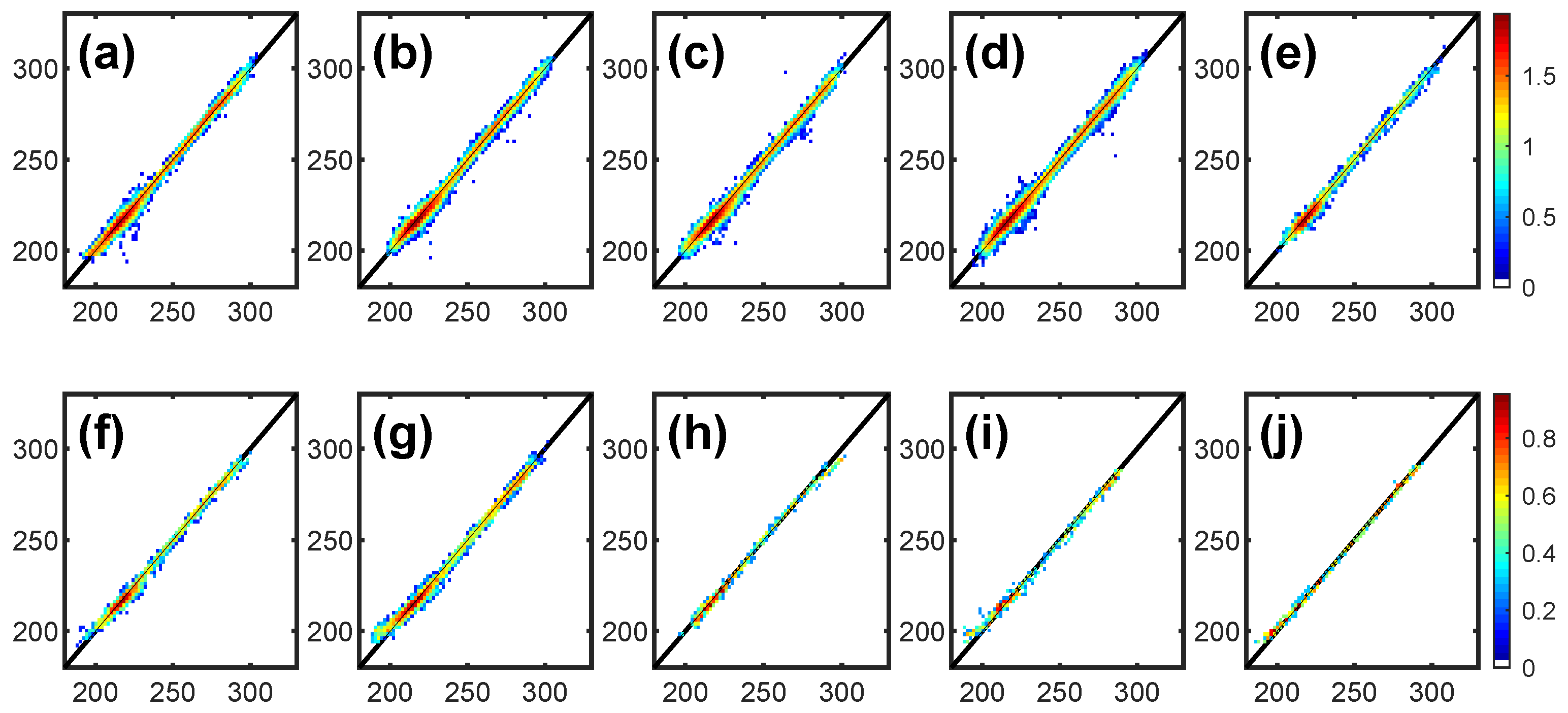
The 2D-histogram plot of the FY4A temperature and radiosonde temperature under the 9 ISCCP cloud types and clear-sky condition. x-axis is the radiosonde temperature, y-axis is FY4A temperature. Units are in K. The cases with QC flags of perfect or good in the vertical range of 10 hPa to surface are selected. The 10 sky conditions are in the 10 sub-figures: (a): clear, with PCC of 0.9959, (b): cirrus, with PCC of 0.9945, (c): cirrostratus, with PCC of 0.9942, (d): deep convection, with PCC of 0.9953, (e): altocumulus, with PCC of 0.9949, (f): altostratus, with PCC of 0.9957, (g): nimbostratus, with PCC of 0.9946, (h): cumulus, with PCC of 0.9967, (i): stratocumulus, with PCC of 0.9943, (j): stratus, with PCC of 0.9912. All the correlation coefficients are at 95% confidence level. The colors represent the frequency 10 where n is the value in color bar. The black line is the identity line.
Figure 5.
The 2D-histogram plot of the FY4A temperature and radiosonde temperature under the 9 ISCCP cloud types and clear-sky condition. x-axis is the radiosonde temperature, y-axis is FY4A temperature. Units are in K. The cases with QC flags of perfect or good in the vertical range of 10 hPa to surface are selected. The 10 sky conditions are in the 10 sub-figures: (a): clear, with PCC of 0.9959, (b): cirrus, with PCC of 0.9945, (c): cirrostratus, with PCC of 0.9942, (d): deep convection, with PCC of 0.9953, (e): altocumulus, with PCC of 0.9949, (f): altostratus, with PCC of 0.9957, (g): nimbostratus, with PCC of 0.9946, (h): cumulus, with PCC of 0.9967, (i): stratocumulus, with PCC of 0.9943, (j): stratus, with PCC of 0.9912. All the correlation coefficients are at 95% confidence level. The colors represent the frequency 10 where n is the value in color bar. The black line is the identity line.

Figure 6.
This figure shows the cases with QC flags of “bad” or “very bad”. The color means the frequency of the observation, 10, n is the value in the color bar. All the observations are shown in this figure except in the unreasonable cases in physics. (a): both clear sky and cloudy sky cases are included, with bias of −3.5 K, RMS of 10.0 K, and PCC of 0.9174; (b): cases under clear sky only, with bias of −0.9 K, RMS of 4.0 K, and PCC of 0.9954; (c): cases under cloudy sky only, with bias of −3.8 K, RMS of 10.4 K, and PCC of 0.9121. All of the correlation coefficients are at 95% confidence level. The black line is the identity line.

Figure 7.
The 2D-histogram plot of the FY4A temperature and radiosonde temperature under the 9 ISCCP cloud types and clear-sky condition. x-axis is the radiosonde temperature, y-axis is FY4A temperature. Units are in K. The cases with QC flags of “bad” or “very bad” in the vertical range of 10 hPa to surface are selected. 10 sky conditions are in the 10 sub-figures: (a): clear, with PCC of 0.9939, (b): cirrus, with PCC of 0.9000, (c): cirrostratus, with PCC of 0.9169, (d): deep convection, with PCC of 0.9174, (e): altocumulus, with PCC of 0.9102, (f): altostratus, with PCC of 0.9463, (g): nimbostratus, with PCC of 0.9072, (h): cumulus, with PCC of 0.9314, (i): stratocumulus, with PCC of 0.9804, (j): stratus, with PCC of 0.9925. All the correlation coefficients are at 95% confidence level. The colors represent the frequency 10 where n is the value in colorbar. The black line is the identity line.

Figure 8.
(a): The vertical distribution of the average RH biases and uncertainties (RMS). The vertical averaged biases, and uncertainties from the surface to 280 hPa (10 km) are shown in panel (a). The biases and uncertainty are based on the absolute error which is the difference from the referenced radiosonde observations. The units are %. The vertical distribution of outlier fractions is shown on the panel (b). The definition of the outlier is that the difference between the FY4A measurements and radiosonde measurements is greater than 35% (or ).

Figure 9.
The 2D-histogram plot of FY4A humidity (y-axis) and radiosonde relative humidity (x-axis) under all-sky (sub-figure (a)), clear sky (sub-figure (b)) and cloudy sky (sub-figure (c)). “all-sky” means the ensemble includes both clear sky and cloudy sky. The plots only contain the cases with quality flags of perfect or good. The color means the frequency of the observation, 10, n is the value in the color bars. All the observations are shown in this figure except the unreasonable cases in physics. (a): all cases are selected, with bias of 0.5%, uncertainty (RMS) of 20% and PCC of 0.6638; (b): cases under clear sky only, with bias of −0.9%, uncertainty (RMS) of 18% and PCC of 0.7113; (c): cases under cloudy sky only, with bias of 0.8%, uncertainty (RMS) of 21% and PCC of 0.6552. The back star points are the average RH of FY4A. Standard error bar is also added to the means of FY4A. The cases in the vertical range from 280 hPa to the surface are selected in the plots. The straight lines are the one-by-one line. Star-line is the average line, and the standard error bars are also added to the start line. All the correlation coefficients are at 95% confidence level. The units are in the absolute value of %. The black line is the identity line.

Figure 10.
The 2D-histogram plot of FY4A relative humidity (y-axis) and radiosonde relative humidity (x-axis). The FY4A RH cases which are labeled with perfect or good in the vertical range from 280 hPa to surface are selected for plots. 10 sky conditions are in the 10 sub-figures: (a): clear, with PCC of 0.7165, (b): cirrus, with PCC of 0.6592, (c): cirrostratus, with PCC of 0.6859, (d): deep convection, with PCC of 0.6593, (e): altocumulus, with PCC of 0.5966, (f): altostratus, with PCC of 0.6605, (g): nimbostratus, with PCC of 0.7231, (h): cumulus, with PCC of 0.3752, (i): stratocumulus, with PCC of 0.7210, (j): stratus, with PCC of 0.8009. All the correlation coefficients are at 95% confidence level. Colors represent the frequency 10 where n is the value in colorbar. The black line is the identity line.


Table 1.
The statistical parameters of the FY4A temperature with QC flags of “perfect” or “good”. The number of cases N, biases () and uncertainties (RMS, ) of the ensembles and sub-ensembles of the FY4A temperature for the different layers and 9 ISCCP cloud types and clear-sky condition. The units of bias and uncertainties are K. total: from the 10 hPa to surface; SL: Stratosphere Layer; TPL: TropoPause Layer; TL: Troposphere Layer; PBL: Planetary Boundary Layer. Ci: Cirrus, CS: cirrostratus, Ac:altocumulus, DC: deep convection, As: altostratus, Ns: nimbostratus, Cu: cumulus, SC: stratocumulus, St:stratus.
| Clear | Ci | Cs | DC | Ac | As | Ns | Cu | Sc | St | |
|---|---|---|---|---|---|---|---|---|---|---|
| N | 15,467 | 15,768 | 19,863 | 32,189 | 3504 | 3048 | 4113 | 727 | 795 | 501 |
| total, | −0.12 | −0.41 | −0.49 | −0.26 | −0.48 | −0.54 | −0.22 | −0.91 | −0.12 | 0.44 |
| 2.59 | 2.89 | 3.05 | 2.72 | 2.70 | 2.58 | 3.12 | 2.40 | 3.65 | 2.58 | |
| N | 4376 | 4593 | 5563 | 9262 | 1022 | 847 | 1208 | 182 | 229 | 138 |
| SL, | −0.43 | −0.60 | −0.90 | −0.47 | −0.89 | −1.05 | 0.23 | −1.86 | 2.02 | 2.40 |
| 3.41 | 3.19 | 3.35 | 3.06 | 2.85 | 3.12 | 4.19 | 2.14 | 4.24 | 3.25 | |
| N | 4187 | 4286 | 5310 | 8724 | 957 | 819 | 1071 | 216 | 197 | 126 |
| TPL, | −0.12 | −0.80 | −0.52 | −0.49 | −0.62 | −0.11 | 0.11 | −0.01 | 0.54 | 0.25 |
| 2.36 | 2.91 | 2.81 | 2.46 | 2.65 | 2.22 | 2.64 | 1.79 | 3.26 | 1.50 | |
| N | 6590 | 6637 | 8477 | 13,507 | 1468 | 1301 | 1681 | 321 | 333 | 217 |
| TL, | 0.05 | −0.06 | −0.26 | −0.02 | −0.14 | −0.49 | −0.78 | −0.94 | −1.90 | −0.69 |
| 1.99 | 2.59 | 2.81 | 2.59 | 2.55 | 2.35 | 2.36 | 2.65 | 2.48 | 1.81 | |
| N | 314 | 252 | 513 | 696 | 57 | 81 | 153 | 8 | 36 | 20 |
| PBL, | 0.36 | 0.75 | 0.33 | 0.64 | 0.46 | −0.27 | 0.05 | −2.41 | −0.97 | 0.33 |
| 2.92 | 2.86 | 4.80 | 2.66 | 3.14 | 2.53 | 2.57 | 2.91 | 2.04 | 1.86 |
Table 2.
The statistical parameters of the FY4A temperature with QC flags of “bad” or “very bad”. The number of cases N, mean bias () and uncertainty (RMS, ) of the ensembles and sub-ensembles of the FY4A temperature for the different layers and 9 ISCCP cloud types and clear-sky condition. The units of bias and uncertainties are K. Total: from the 10 hPa to surface; SL: Stratosphere Layer; TPL: TropoPause Layer; TL: Troposphere Layer; PBL: Planetary Boundary Layer. Ci: Cirrus, CS: cirrostratus, Ac:altocumulus, DC: deep convection, As: altostratus, Ns: nimbostratus, Cu: cumulus, SC: stratocumulus, St:stratus.
| Clear | Ci | Cs | DC | Ac | As | Ns | Cu | Sc | St | |
|---|---|---|---|---|---|---|---|---|---|---|
| N | 10,221 | 11,725 | 14,829 | 22,404 | 2824 | 2061 | 3388 | 497 | 653 | 358 |
| total, | −3.36 | −4.34 | −4.33 | −4.31 | −6.33 | −3.65 | −2.95 | −6.09 | −2.25 | 0.18 |
| 8.99 | 10.95 | 10.49 | 10.02 | 10.39 | 8.22 | 12.09 | 9.78 | 6.21 | 4.31 | |
| N | 3881 | 4414 | 5121 | 8490 | 1005 | 755 | 1125 | 162 | 216 | 118 |
| SL, | −3.19 | −4.09 | −4.22 | −3.71 | −6.09 | −4.26 | −2.52 | −8.98 | 0.79 | 3.63 |
| 9.06 | 10.78 | 9.04 | 8.70 | 10.90 | 8.43 | 10.11 | 8.84 | 7.09 | 3.46 | |
| N | 2933 | 3748 | 4296 | 6969 | 929 | 549 | 905 | 157 | 163 | 82 |
| TPL, | −3.72 | −5.70 | −4.13 | −5.15 | −8.38 | −2.61 | −1.06 | −4.46 | −0.93 | 0.35 |
| 9.38 | 12.13 | 11.91 | 11.61 | 10.55 | 9.75 | 14.58 | 8.95 | 5.32 | 3.88 | |
| N | 3000 | 3423 | 4904 | 6404 | 860 | 685 | 1218 | 177 | 240 | 126 |
| TL, | −3.55 | −3.35 | −4.92 | −4.56 | −4.58 | −3.99 | −4.94 | −4.92 | −5.89 | −3.15 |
| 8.93 | 9.69 | 10.80 | 9.88 | 9.29 | 6.79 | 12.03 | 10.73 | 3.77 | 2.97 | |
| N | 407 | 140 | 508 | 541 | 30 | 72 | 140 | 1 | 34 | 32 |
| PBL, | −0.96 | 0.01 | −1.61 | 0.02 | −1.63 | −1.92 | −1.23 | −2.08 | −2.28 | 0.09 |
| 4.19 | 6.36 | 7.16 | 6.85 | 5.20 | 2.71 | 4.43 | 0 | 5.13 | 1.69 |
Table 3.
The number of cases N, mean bias () and uncertainty (RMS, ) of the ensembles and sub-ensembles of the FY4A humidity for the layer from 280 hPa to the surface and 9 ISCCP cloud types. The FY4A humidity is with a quality flag of “perfect” and “good” only. The units of bias and uncertainties are the absolute value of %. Ci: Cirrus, CS: cirrostratus, Ac:altocumulus, DC: deep convection, As: altostratus, Ns: nimbostratus, Cu: cumulus, SC: stratocumulus, St:stratus.
| Clear | Ci | Cs | DC | Ac | As | Ns | Cu | Sc | St | |
|---|---|---|---|---|---|---|---|---|---|---|
| N | 6204 | 6079 | 8091 | 12479 | 1307 | 1235 | 1672 | 268 | 333 | 209 |
| −0.9 | 1.4 | 0.1 | 0.5 | 4.3 | 1.3 | 0.9 | 2.5 | 0.7 | 1.5 | |
| 18.3 | 20.6 | 19.4 | 21.3 | 21.1 | 20.6 | 21.3 | 27.9 | 22.3 | 16.0 |
© 2019 by the authors. Licensee MDPI, Basel, Switzerland. This article is an open access article distributed under the terms and conditions of the Creative Commons Attribution (CC BY) license (http://creativecommons.org/licenses/by/4.0/).
Share and Cite
MDPI and ACS Style
He, M.; Wang, D.; Ding, W.; Wan, Y.; Chen, Y.; Zhang, Y. A Validation of Fengyun4A Temperature and Humidity Profile Products by Radiosonde Observations. Remote Sens. 2019, 11, 2039. https://doi.org/10.3390/rs11172039
AMA Style
He M, Wang D, Ding W, Wan Y, Chen Y, Zhang Y. A Validation of Fengyun4A Temperature and Humidity Profile Products by Radiosonde Observations. Remote Sensing. 2019; 11(17):2039. https://doi.org/10.3390/rs11172039
Chicago/Turabian StyleHe, Min, Donghai Wang, Weiyu Ding, Yijing Wan, Yonghang Chen, and Yu Zhang. 2019. "A Validation of Fengyun4A Temperature and Humidity Profile Products by Radiosonde Observations" Remote Sensing 11, no. 17: 2039. https://doi.org/10.3390/rs11172039
Note that from the first issue of 2016, this journal uses article numbers instead of page numbers. See further details here.