Semi-Supervised PolSAR Image Classification Based on Self-Training and Superpixels
by
Yangyang Li
1,*, 
Ruoting Xing
1,
Licheng Jiao
1,
Yanqiao Chen
1,
Yingte Chai
1,
Naresh Marturi
2 and
Ronghua Shang
1 1
Key Laboratory of Intelligent Perception and Image Understanding of Ministry of Education, International Research Center for Intelligent Perception and Computation, Joint International Research Laboratory of Intelligent Perception and Computation, Xidian University, Xi’an 710071, Shaanxi Province, China
2
Extreme Robotics Laboratory, University of Birmingham, Edgbaston B15 2TT, UK
*
Author to whom correspondence should be addressed.
Remote Sens. 2019, 11(16), 1933; https://doi.org/10.3390/rs11161933
Submission received: 24 June 2019
/
Revised: 28 July 2019
/
Accepted: 12 August 2019
/
Published: 19 August 2019
(This article belongs to the Section Remote Sensing Image Processing)
Abstract
:Polarimetric synthetic aperture radar (PolSAR) image classification is a recent technology with great practical value in the field of remote sensing. However, due to the time-consuming and labor-intensive data collection, there are few labeled datasets available. Furthermore, most available state-of-the-art classification methods heavily suffer from the speckle noise. To solve these problems, in this paper, a novel semi-supervised algorithm based on self-training and superpixels is proposed. First, the Pauli-RGB image is over-segmented into superpixels to obtain a large number of homogeneous areas. Then, features that can mitigate the effects of the speckle noise are obtained using spatial weighting in the same superpixel. Next, the training set is expanded iteratively utilizing a semi-supervised unlabeled sample selection strategy that elaborately makes use of spatial relations provided by superpixels. In addition, a stacked sparse auto-encoder is self-trained using the expanded training set to obtain classification results. Experiments on two typical PolSAR datasets verified its capability of suppressing the speckle noise and showed excellent classification performance with limited labeled data.
1. Introduction
Synthetic aperture radar (SAR) is a prominent technology for acquiring terrain information, which can provide high-resolution images in all weather conditions, independent of day and night. Polarimetric SAR (PolSAR), in addition to the characteristics mentioned above, is able to use the backscattering of polarization waves from objects to form images. In recent years, research on PolSAR has attracted wide interest in the field of remote sensing, and applications of PolSAR images have gradually increased, such as crop classification [1], ship detection [2], and change detection [3]. PolSAR image classification assigns a specific ground category to each pixel. Broadly, classification methods of PolSAR images can be divided into the categories listed below.
Many frequently used classification methods are based on target decomposition, such as Pauli decomposition [4], entropy/alpha (H/α) decomposition [5], Freeman decomposition [6] and Yamaguchi decomposition [7]. Target decompositions provide sound theories, so they have been widely studied [8,9]. Furthermore, the statistical distribution of PolSAR data is used for classifying PolSAR images. It is known that both the covariance matrix and the coherence matrix of each pixel in homogeneous areas have a complex Wishart distribution. Li Zhong Sen et al. [10] proposed a method based on the Wishart distance for PolSAR image classification. Since then, the Wishart distance and its variants have become the choice for measuring similarities among pixels in many studies [11,12].
The above two methods are generally performed as an unsupervised classification. However, results of these methods are usually rough because they cannot distinguish different kinds of regions with similar characteristics well, or the same kind of region with certain different characteristics, so more guide information is needed to perform better classification. Supervised learning has recently become mainstream in PolSAR classification. It requires training samples with complete labels, thus further improving the classification accuracy.
Traditional supervised machine learning, which does not include deep learning, is frequently involved in PolSAR classification. One popular machine learning model is the support vector machine (SVM) [13], which has been proved to be effective in the field of artificial intelligence and pattern recognition. In addition, ensemble learning such as random forest [14] is also utilized. In 2006, Hinton et al. [15] proposed an epoch-making work on deep belief networks (DBN). In 2012, Krizhevsky et al. [16] applied a convolutional neural network (CNN) for ImageNet classification and achieved eminent results. Since then, deep learning has been accepted as a popular technique, the main advantage of which is automatic and hierarchical feature extraction. As one of the deep learning models, sparse auto-encoders (SAEs) have been successfully applied to PolSAR classification [17,18,19,20]. However, these methods process each pixel in isolation and utilize a small number of training samples, severely suffering from speckle noise and over-fitting. Although supervised methods can effectively improve the classification accuracy, the demand for robust feature representation and a large number of labeled samples remains to be solved.
Semi-supervised learning has been increasingly introduced into the field of remote sensing [21,22,23] in order to alleviate the problems mentioned above. Semi-supervised classification utilizes unlabeled samples to expand training sets, which greatly contributes towards overcoming over-fitting and achieving a better classification accuracy. In general, semi-supervised classification can be divided into five categories, including generation models [24], self-training models [25], co-training models [26], tranductive SVMs [27], and graph-based models [28]. Among all the semi-supervised models, the self-training model, the co-training model and the graph-based model are the most frequently used in PolSAR classification. A semi-supervised PolSAR classification method based on improved co-training has been proposed in the literature [26]. Two sufficient and conditionally independent views were constructed for the co-training process based on features of PolSAR images, and a novel sample selection strategy for selecting reliable unlabeled samples is used to update this process. The algorithm achieves acceptable classification accuracy with limited labeled samples. Recently, the good performance of graph-based semi-supervised models has been proved in PolSAR classification. In [28], the authors constructed a spatial-anchor graph to implement sparse representation of the feature space, and propagated category labels on the edge of the graph based on similarities of nodes of labeled samples and unlabeled samples to implement semi-supervised classification.
For graph-based semi-supervised classification, the construction of the graph is fairly complex, and label propagations rely on the inversion of a large matrix, which limits their application for remote sensing applications [29]. As for co-training models, it is difficult to obtain sufficient and conditionally independent views. Semi-supervised learning based on self-training is promising. The idea is simple and efficient. Usually, a classifier, for example, a machine learning model or a deep learning model, is initialized first. Then unlabeled samples are selected to add to the training set according to similarities with neighboring labeled training samples. The classifier updates itself with the expanded training set to improve the classification accuracy. The key for self-training is to formulate an unlabeled sample selection strategy that can contribute to the training process.
In [25], the authors proposed a superpixel restrained deep neural network with multiple decisions (SRDNN-MD). The proposed semi-supervised unlabeled sample selection strategy named multiple decisions (MD) include nonlocal decisions and local decisions. The nonlocal decision sets each label the training sample as the center of the nonlocal region. Then, similarities are determined jointly by the cosine distance, and the output prediction probability of the deep neural network is measured to select the most similar unlabeled sample. As for the local decision, each unlabeled sample is set as the center of a local region. Similarities between labeled training samples located in the local region and the unlabeled sample are measured by the spatial distance and the output prediction probability of the deep neural network. Finally, unlabeled samples are labeled as the same class as training samples according to similarities measured by nonlocal and local decisions. In addition, SRDNN-MD designs a superpixel-restrained term for the deep neural network to enhance the homogeneous characters of the same superpixel and reduce the impacts of the speckle noise. Another study [29] proposed a bagging ensemble-based self-training method. In this method, when both the reliability and diversity of the selected samples are taken into account, the initial classifier should find samples that do not necessarily have the highest prediction probability. Two search strategies to select candidate unlabeled samples are considered and evaluated. One is to limit the search neighborhood around all labeled samples. The other is to set the search neighborhood around labeled samples of a particular category. Then, search areas of these two strategies iteratively grow until the entire image is covered.
This paper proposes a novel semi-supervised PolSAR classification method based on self-training and superpixels. One important motivation of this work is the similarity and continuity inside each superpixel. First, the RGB PolSAR image that is formed by Pauli decomposition is over-segmented into superpixels by the simple linear iterative clustering (SLIC) algorithm [30]. Then, we extract features of each pixel from its coherence matrix. To mitigate the effects of speckle noise, features of each pixel are re-represented using spatial weighting with its neighboring pixels in the same superpixel. Next, we propose a semi-supervised unlabeled sample selection method for expanding training sets. Label propagations for unlabeled samples can be guided well by our strategy. Finally, a self-training stacked sparse auto-encoder (SSAE) network iteratively updates itself with the expanded training set and generates the global classification map of the PolSAR image. In contrast to SRDNN-MD, which only selects the most reliable samples according to similarity metrics computed by local and nonlocal decisions, the proposed sample selection procedure ensures both the reliability and diversity of the selected unlabeled samples and makes the most of the similarity and continuity inside each superpixel to save required computations. The proposed procedure is also more concise than the procedure in [29] because we do not need to grow the search region for unlabeled sample selections iteratively. Each superpixel is utilized only once to select samples. Moreover, we choose a single strong classifier rather than multiple weak classifiers to perform the PolSAR classification. Several groups of experiments were implemented on two representative PolSAR datasets and we obtained impressive results on the proposed self-training-based semi-supervised PolSAR classification.
The remainder of this paper is organized as follows. Section 2 introduces components and the whole framework of the algorithm. Section 3 compares the proposed algorithm with some existing PolSAR classification algorithms on two datasets to verify its effectiveness. Section 4 discusses the parameter choices and experimental results in Section 3. Section 5 summarizes the full text and proposes further work to be studied in the future.
2. Methodology
2.1. Superpixel Segmentation
As an important branch in the field of segmentation, superpixels were first proposed by Ren et al. in 2003 [31]. They were originally designed as preprocessing for optical images. Superpixels over-segment the image into homogeneous pixel blocks with adjacent positions and similar features. In recent years, it has become a promising technology in PolSAR image classification [32,33]. It is known that pixels within the same superpixel may share the same category to some extent, which may simplify the subsequent steps of the classification tasks.
The SLIC [30] algorithm is utilized to generate superpixels in this paper. Compared with other algorithms [34,35,36], SLIC generates regular superpixels with high boundary adherence and it implements them much more rapidly, using simple and efficient modified k-means clustering. Centers and their neighboring pixels in each superpixel are alternately updated according to a distance measure. Suppose [, , , , ] and [, , , , ] are vectors of two pixels. L, A and B are the luminance component and two color components of the LAB color space, respectively. X and Y are spatial coordinates. Then the distance measure between two pixels is calculated as:
where
where and are the LAB color distance and the spatial distance of the two pixels, respectively. m is the constant parameter that weighs the importance of and . r is the pixel interval for producing roughly equally-sized superpixels. , where is the number of image pixels and n is the number of superpixels. The steps of the SLIC algorithm are summarized below.
| Algorithm 1: SLIC |
| Input: The RGB PolSAR image, the number of superpixels n, threshold e. |
| 1: Evenly initialize n cluster centers by sampling pixels with interval r. Then cluster centers are moved to seed locations where the lowest gradient meets in a 3×3 neighborhood. do: |
| 2: Search pixels in a 2r×2r region around each cluster center and calculate the distance measure from each searched pixel to the cluster center using (1), (2) and (3). |
| 3: Assign searched pixels to superpixels that involve the nearest cluster center. |
| 4: Calculate the average vector of each superpixel as the new cluster center. 5: Compute the residual error between the new cluster center and the previous cluster center using L2 norm. while the residual error > e |
| 6: Check the number of pixels in each superpixel. If it is less than n/4, merge this superpixel with its adjacent one. Output: The over-segmented PolSAR image with around n superpixels. |
2.2. Feature Representation of PolSAR Images
According to the polarizations of transmitted and received waves, the PolSAR system works in four polarization modes: HH, VV, HV, VH. The polarization scattering matrix is used to represent the scattering characteristics of each pixel, which contain all the information about the target.
Each scattering parameter in the matrix is a complex number. The scattering matrix is decomposed into a complex weighted sum of Pauli matrices, which is called Pauli decomposition. In the case of reciprocal backscattering , the scattering matrix can be expressed as:
where
In this paper, the RGB image is formed by Pauli decomposition, whose three channels are , and . The complex polarization vector is . If the PolSAR data are multi-look processed for speckle reduction, the coherence matrix, which can also represent a pixel, is obtained as follows:
where indicates the th sample of vector , the symbol * indicates the complex conjugate, and is the number of looks.
In addition, polarimetric characteristics can be extracted through target decomposition theories that reveal the invariance of polarization characteristics of the target under different wave polarization bases [8]. The Yamaguchi decomposition [7] theorem decomposes T into four scattering powers, named as the volume scattering (), the double-bounce scattering (), the surface scattering () and the helix scattering (), respectively. In this paper, each pixel is represented by a 10-dimension feature vector that is made up of components of T and the Yamaguchi decomposition:
In order to mitigate the effects of speckle noise on the classification map, the spatial weighting method is utilized in our approach. For a specific pixel p whose feature vector is , we randomly choose pixels that are in the same superpixel as pixel p. If we suppose that features of these neighboring pixels are , then the spatial weighting feature can be obtained as follows:
It is worth noting that the size of each superpixel may vary within certain ranges, so it is important to find a reasonable number of neighboring pixels , which will be further discussed in the experiment section.
2.3. Semi-Supervised Unlabeled Sample Selection Based on Superpixels
As mentioned in Section 1, in practical applications, to obtain a large number of labeled samples is time-consuming and labor-intensive. In PolSAR classification, because high resolution PolSAR images are usually obtained from a few national key laboratories with specific PolSAR sensor systems, and many experts are required to collect and label the original image, labeled data is even less, which limits the classification accuracy and generalization ability of models. Semi-supervised learning provides a compromise for this problem. It detaches the whole learning process from an interaction with the outside world and automatically uses unlabeled samples to improve the learning performance.
To take advantage of unlabeled samples, one motivation for our work is the "cluster assumption", that is, samples of the same cluster have a high probability of belonging to the same category. In this paper, superpixel segmentation is implemented to over-segment the image into many homogeneous clusters, so we utilize spatial relations obtained from superpixels along with prediction probabilities obtained from the classifier to propagate labels from labeled samples to unlabeled samples.
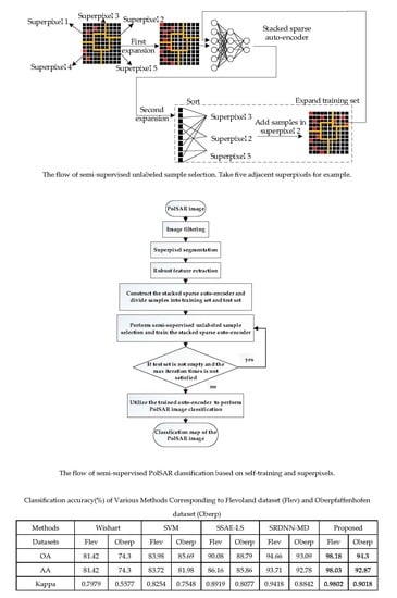
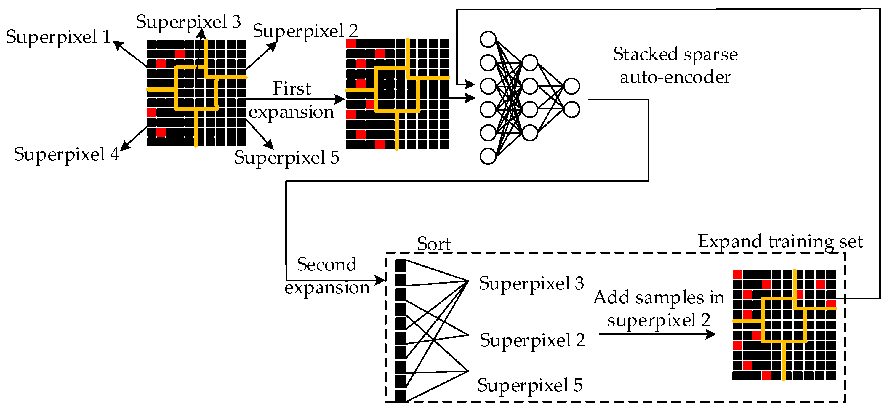
The method is illustrated in Figure 1. In detail, the accurately-labeled sample set of the PolSAR image should be obtained first. Then we randomly select a certain number of pixels from each class to form the initial training set , which is expressed as , where involves labeled training samples belonging to the th class, , N is the number of categories of the PolSAR image. Remaining pixels in the PolSAR image are added to the candidate unlabeled sample set and the test set identically. is utilized to expand the training set, and is utilized to evaluate the classification performance.
Next, two expansions on the training set are performed in sequence. The first expansion is implemented as follows for each class:
- For each sample in belonging to class , assuming that the sample is located in the superpixel , randomly select unlabeled pixels in and take as the label of these pixels. Then add samples in and selected pixels in to a new training set, named , where t indicates iteration times.
- All pixels in are removed from , which indicates that superpixel has been traversed.
Input the training set into the classifier and train it for the first time. Then the classifier makes predictions on . Assuming that , where indicates the set of samples with prediction , where , the output probability of the classifier that corresponds to the predicted class is considered as the prediction confidence of each candidate unlabeled sample in . Next, we perform the second expansion on with the following steps for each class:
- For all samples in predicted as class , sort their prediction confidence from high to low. Select unlabeled samples with the highest confidence and combine them into a set, named .
- For each sample of , record the superpixel in which it falls. Count the number of samples that fall in different superpixels. The superpixel with the minimum number of samples is selected, which is recorded as .
- Randomly select samples in , and take as the label of these samples. Add them to the training set and remove all pixels in from , which indicates that superpixel has been traversed.
Afterwards, we perform the second expansion on the training set iteratively and train the classifier iteratively. The process may finish by following two conditions. One is that the unlabeled sample set becomes empty so that the training set fails to expand. The other is to set the maximum iteration time as .
The proposed semi-supervised unlabeled sample selection method ensures both the reliability and diversity of the selected unlabeled samples. On the one hand, each superpixel is only traversed once to select unlabeled samples. The remaining candidate samples in the same superpixel are removed from . We choose the most representative samples, which can enhance the reliability and diversity of unlabeled sample selection and accelerate the training process.
On the other hand, the procedure of two expansions on the training set also balances the reliability and diversity of the selected unlabeled samples. In the first expansion, we use the "clustering assumption" to directly propagate labels to samples in the same superpixel. In the second expansion, we first obtain candidate samples from whose prediction confidences range from 1 to . Their confidences are high enough to guarantee the reliability. Then, we choose the superpixel that contains the minimum number of samples, which means samples within this superpixel are of great diversity. Therefore, these samples have potential to improve the classification performance.
In summary, the semi-supervised unlabeled sample selection method based on superpixels provides a novel and effective strategy for expanding training sets with unlabeled samples of great reliability and diversity, which fully utilizes the results of superpixel segmentation and the potential of semi-supervised learning.
2.4. Self-Training SSAEs
In is paper, we choose SSAE as the self-training classifier. Many characters of SSAE are adapted to PolSAR classification. It automatically generates low dimensional hidden-layer feature representations for each input pixel, which is suitable for pixel classification of PolSAR images. SSAEs are generally shallow networks with a small number of parameters, so that it protects the training from over-fitting. The training of SSAE includes unsupervised layer-by-layer greedy training and supervised fine-tuning.
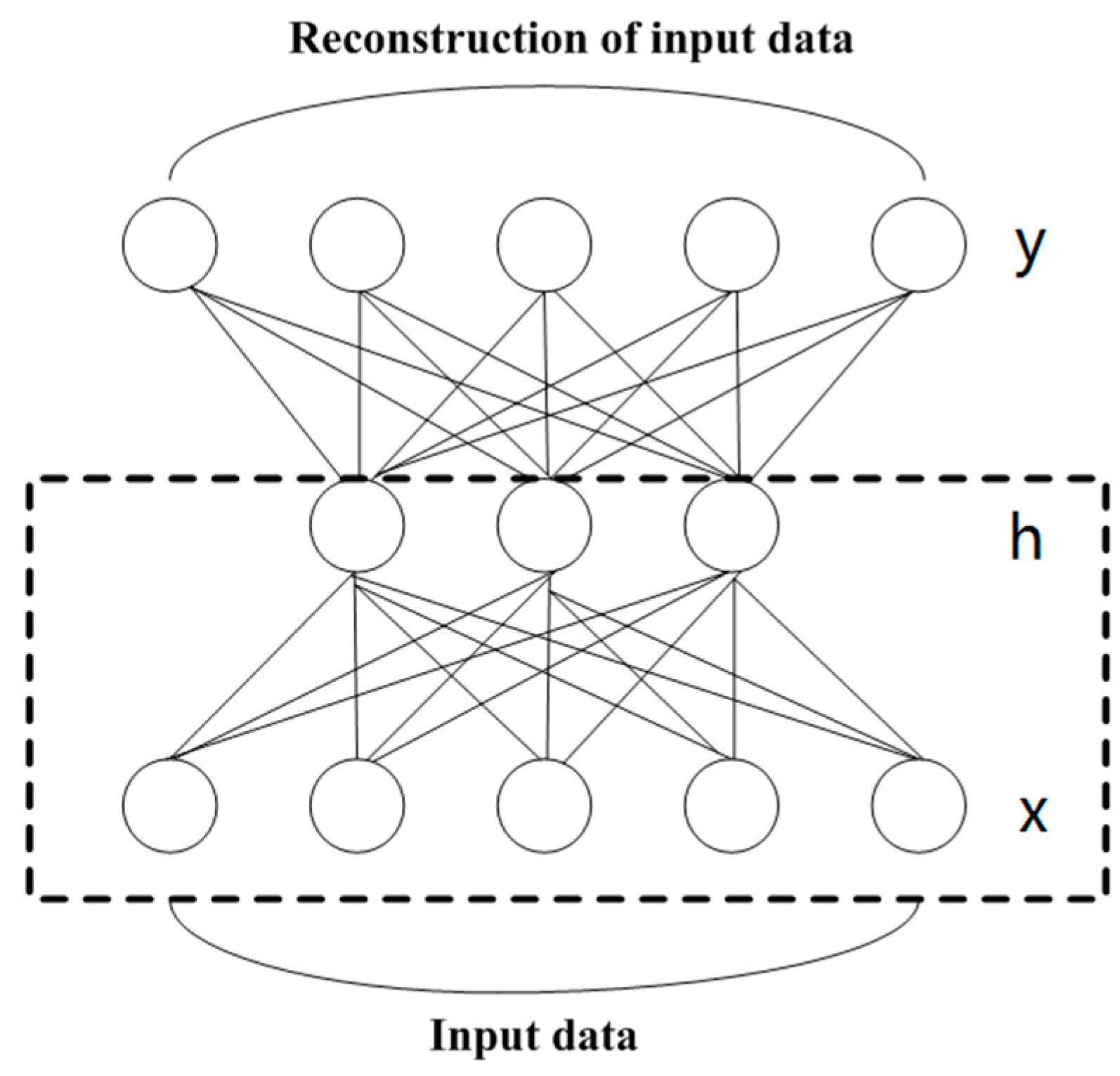
Figure 2 shows the structure of an SAE composed of an input layer, a hidden layer and a reconstruction layer. The number of neurons in the input layer and the reconstruction layer are the same. The data at the second layer is the hidden feature vector learned by the SAE. If there is a sample x, the hidden expression h can be obtained as follows:
Later, the h is decoded according to the formula given by (11) and the reconstruction y is obtained:
where W and b are the weight matrix and bias vector, respectively. f() and g() are activation functions. The corresponding error function minimizing the difference between x and y is given by:
In order to get a compressed representation of , we must perform a sparse restriction on the hidden layer. According to (13), the mean squared-error function of the SAE can be obtained as:
where M is the number of samples, is the sparse parameter, is the average activation of the jth hidden neuron and h is the number of the hidden neurons. The KL divergence can be expressed as follows:
when the above error function (13) is at its minimum, the data of the hidden layer becomes an excellent feature of input sample x.
When performing layer-by-layer greedy training for SSAE with several hidden layers, the feature vector of the first hidden layer is learned at first, then it is input into the next hidden layer. The process is repeated several times until all layers are trained. Next, a soft-max classifier is applied to produce the prediction probability distributions. The soft-max classifier is expressed as follows:
where is a trainable parameter, and q is the number of classes. When performing fine-tuning, the parameters of SSAEs are adjusted by the back propagation (BP) algorithm. Then, the trained network can be used for prediction and classification. The loss function is the cross entropy given by:
where, 1{} is the indicator function.
2.5. Procedure of the Proposed Algorithm
As described above, the proposed semi-supervised PolSAR classification algorithm firstly constructs a real feature vector that suppresses the speckle noise of each pixel based on the superpixel segmentation result. Then, an SSAE is trained with a few training samples. A series of superpixel-inspired methods are utilized to iteratively select reliable unlabeled samples according to their prediction confidences, using our two expansions on the training set. The classifier has already fitted those samples with high confidence well, so we take both the reliability and diversity of the samples into account. Next, the SSAE is iteratively self-trained using the expanded training set.
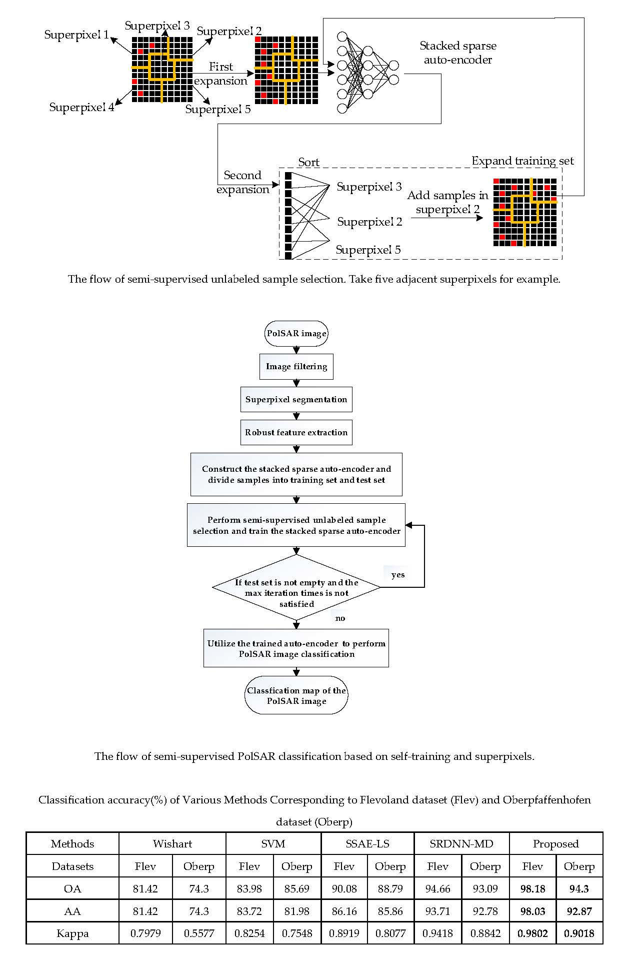
In summary, the description of the whole algorithm is given below.
| Algorithm 2: Semi-supervised PolSAR classification based on self-training and superpixels |
| Input: The RGB PolSAR image. 1: The PolSAR image to be classified is filtered using the Lee refined filtering algorithm. |
| 2: Segment the Pauli RGB pseudo color image using the SLIC superpixel algorithm. |
| 3: Construct feature representation for each pixel in the PolSAR image. Calculate new feature representation that can suppress the speckle noise for each pixel p using spatial weighting. |
| 4: Prepare the initial training set , the candidate unlabeled sample set and the test set . Construct the self-training SSAE for classification. Set iteration times t = 0. while is not empty and : |
| 5: Perform semi-supervised unlabeled sample selection and obtain the expanded training set . |
| 6: Use to train the SSAE. end while |
| 7: Use to evaluate the classification performance of the method and utilize the trained auto-encoder to perform PolSAR image classification. Output: The classification map of the PolSAR image. |
3. Experimental Results
In this section, we will verify the effectiveness of the proposed algorithm on two PolSAR datasets. In Section 3.1, we introduce the data set and parameter settings used in the experiment. Section 3.2 and Section 3.3 show the classification results of the algorithm compared with other popular PolSAR classification algorithms on two datasets, respectively.
3.1. Datasets and Parameter Settings
In this experiment, we used several typical datasets to test the performance of different algorithms. The first one was the L-band Flevoland data obtained by the NASA AIRSAR sensor in the United States. The size of the image is 750*1024 pixels. It mainly consists of 15 kinds of land cover categories, including water, barley, peas, stembeans, beet, forest, bare soil, grasses, rapeseed, lucerne, wheat 1, wheat 2, building, potato, and wheat 3. Figure 3a shows the Pauli-RGB image of the data and Figure 3b shows the ground-truth. Figure 3i shows the color code. The second one was the L-band Oberpfaffenhofen data, which is acquired by the ESAR sensor of DLR in Germany. The size is 1300×1200 pixels. There are three categories in the image, including a built-up area, woodland and open area. Figure 7a,b respectively show the Pauli-RGB image and the ground-truth. Figure 7i shows the color code. In the proposed algorithm, all images are filtered by the Lee refined filter with the window size of 7. The SSAE constructed in this paper is composed of two hidden layers and a softmax layer. The number of neurons in each layer are 150 and 40, respectively, according to [25]. The learning rate in layer-by-layer greedy training is set to 0.02 and 0.2, respectively. While in fine-tuning, the learning rate is set to 0.1. The former and the latter iterates 30 and 200 times, respectively, with a stochastic gradient descent algorithm. The sigmoid function is adopted as the activation function. The maximum iteration times of semi-supervised unlabeled sample selection is 20 for the Flevoland data and 12 for the Oberpfaffenhofen data. As for some important parameters such as the number of superpixels n, , , , we will show their influences in detail in the discussion section.
Four kinds of compared algorithms that have various different degrees of supervision are also implemented in this paper, including the unsupervised complex Wishart classifier [10], supervised algorithms such as SVM [13], the stacked sparse auto-encoder in PolSAR classification using local spatial information (SSAE-LS) [19], and semi-supervised algorithms such as SRDNN-MD [25]. Spatial weighting feature vectors introduced in Section 2.2 were utilized in all compared algorithms. Parameters of SSAE used in compared algorithms were set to the same parameters as the proposed algorithm so as to compare them as fairly as possible, and the remaining parameters follow the original paper. We used multi-classification SVM, whose kernel is the radial basis function. The penalty coefficient C and the parameter γ were set to 32 and 0.25 for the Flevoland data and 32 and 32 for the Oberpfaffenhofen data, which were optimized by cross validation.
All the experiments in this paper were implemented in MATLAB R2016b, with Intel Core i5-6500 3.2-GHz CPU and 8-GB memory.
3.2. Experiment on Flevoland Data
Extensive experiments were implemented on the Flevoland dataset to verify the effectiveness and superiority of the proposed algorithm. We randomly chose 1% of the samples for each category and combined them into the initial training set. Table 1 compares the quantity of training samples and that of ground truth intuitively. Classification results are shown in Figure 3. Figure 3c shows the map of superpixel segmentation. Figure 3d–g show classification maps obtained by Wishart, SVM, SSAE-LS and SRDNN-MD. Figure 3h shows the classification map obtained by the proposed algorithm.
Overall, the regional consistency of the maps obtained by Wishart and SVM are very poor. Two algorithms were both severely affected by the speckle noise, as Figure 3d,e show. It is obvious that Wishart severely confuses bare soil, grasses, and water. Particularly, there are few pixels that fall into the bare soil category. SVM also performs poorly on the grasses category. In addition, SVM can hardly distinguish potatoes from forest, and there are several misclassifications corresponding to other categories on the two maps. The classification map of SSAE-LS seems a little better. However, the algorithm has not performed well on the buildings category due to the low sampling rate of the Flevoland data, and there is insufficient speckle noise removal in the local domain.
As shown by Figure 3g,h, the two semi-supervised algorithms, SRDNN-MD and the proposed algorithm, have alleviated the problems mentioned above to a great extent, and there are fewer visible misclassifications. The classification map of the proposed algorithm is a lot better than the one of SRDNN-MD as it is almost unaffected by the speckle noise. In particular, the map of SRDNN-MD has blurred edges, while the map of the proposed algorithm has clearer edges, which enhance the regional consistency of the same category. These observations fully demonstrate that we have propagated appropriate labels to unlabeled samples, and these samples can effectively improve the performance.
In order to evaluate the classification performance quantitatively, three evaluation indexes that are widely used in the field of remote sensing are adopted, namely overall accuracy (OA), average accuracy (AA) and Kappa. Table 2 shows the evaluation results of each class and the overall classification performance. The bold font indicates the optimal result of each row. It can be seen that the experimental data consists of what we have seen on the classification maps obtained above. At the sampling rate of 1%, expect for the water category, the proposed algorithm realizes optimal results in all evaluation indexes, the OA value of which is as high as 98.18%. The classification accuracy of each category is above 96%, except for the grasses category. This excellent performance is far better than the second best performance of SRDNN-MD, whose OA is 94.66%. The OA values of Wishart and SVM are no more than 90%. Although their parameters are elaborately optimized by cross validation, the classification results of each category have great differences. SSAE-LS performs poorly on buildings and grasses, the OA value of which is a little more than 90%. We can also infer that bare soil, grasses and water are hard categories to distinguish well.
To summarize, the proposed semi-supervised PolSAR image classification algorithm based on self-training and superpixels obtained a more superior performance on the Flevoland dataset compared with the other algorithms, which proves the effectiveness of the method.
3.3. Experiment on Oberpfaffenhofen Data
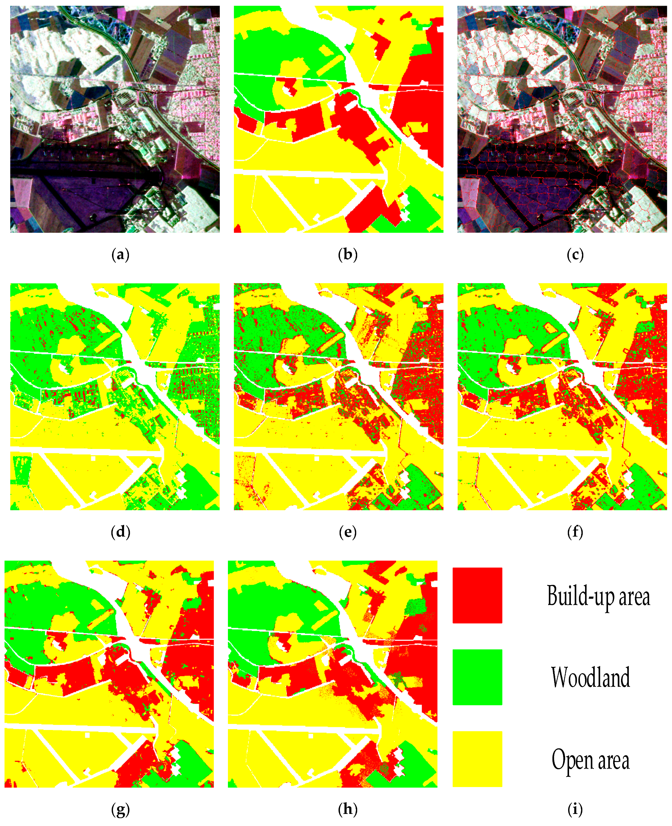
To further evaluate the classification capability of the proposed algorithm on PolSAR data, we also performed experiments on Oberpfaffenhofen data. We randomly chose 1000 samples for each category and combined them into the initial training set. Table 3 compares the quantity of training samples and that of the ground truth intuitively. Figure 4c shows homogeneous blocks obtained by superpixel segmentation. Figure 4d–g show classification maps obtained by the compared algorithms. Figure 4h is the classification map obtained by the proposed algorithm. Table 4 shows the test results in the classification performance of different categories and the overall classification performance. The bold font indicates the optimal value of each row.
It can be seen from Figure 4d and Table 4 that the classification performance of Wishart is very poor, and can hardly recognize built-up areas. SVM and SSAE-LS obviously improve the recognition accuracy of built-up areas, but pixels of built-up areas appear as dense noise in their corresponding classification maps as well. Next, we focus on results obtained by the two semi-supervised algorithms. The proposed algorithm shows a greater ability to suppress noise and the particle size of noise in the proposed algorithm is much smaller than SRDNN-MD, which maintains good intra-class consistency.
The same conclusion can be obtained by Table 4. The overall accuracy of the proposed algorithm is as high as 94.3%, which is 27%, 10%, 6.2%, and 1.3% higher than the compared algorithms, respectively. The proposed algorithm realizes the best accuracies on woodland and open areas. As shown in experiments on Flevoland, SRDNN-MD always confuses different categories on both sides of edges, so its classification performance is not as good as the proposed algorithm. Note that the proposed algorithm is not so good at recognizing built-up areas, but the result is close to the best accuracy. Overall, the proposed algorithm is superior to SRDNN-MD in most evaluation indexes, which proves that the semi-supervised PolSAR classification algorithm based on self-training and superpixels can be effectively generalized to different datasets and can obtain a competitive classification performance.
4. Discussion
4.1. Parameter Analysis
There are four significant parameters in the proposed algorithm, including the number of superpixels n, , and . We perform the following three group of experiments in this section to analyze the proper parameter choices, taking the classification of the Flevoland data as an example.
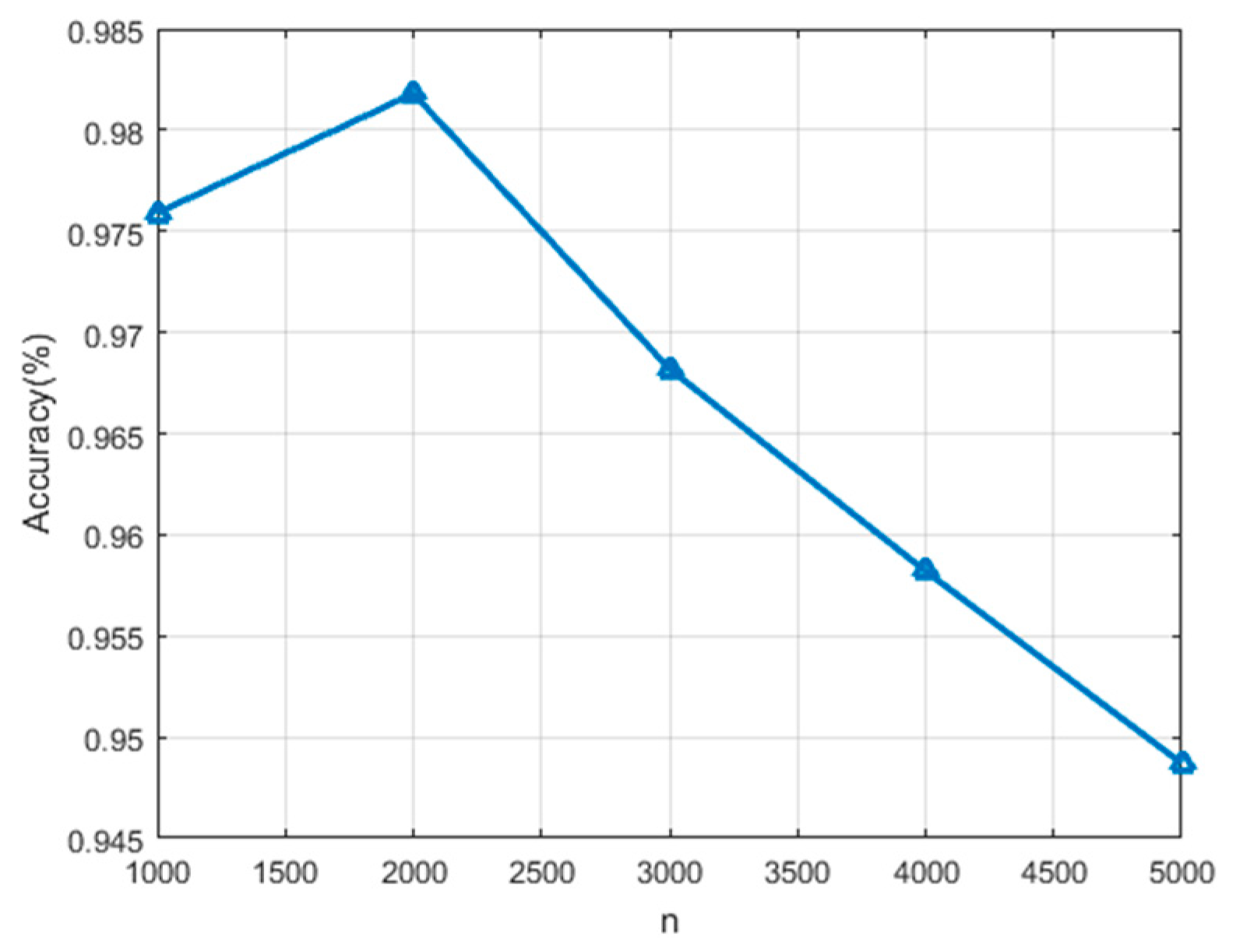
The first group of experiments discuss the effect of the number of superpixels on the classification performance. The discussed parameter n ranges from 1000 to 5000, and the interval is 1000. Other parameters are kept unchanged in this discussion. The experiment results are shown in Figure 5. The best classification accuracy is obtained when n is set to 2000. We infer that if the parameter is too large, the number of pixels contained in each superpixel will reduce, which is not conducive to eliminating the speckle noise, and is not conducive to performing the proposed semi-supervised unlabeled sample selection method because the diversity of samples may be lost. In contrast, if the parameter is set too small, the number of pixels contained in each superpixel will increase, which is likely to propagate incorrect labels to the selected unlabeled samples, thus reducing the classification accuracy.
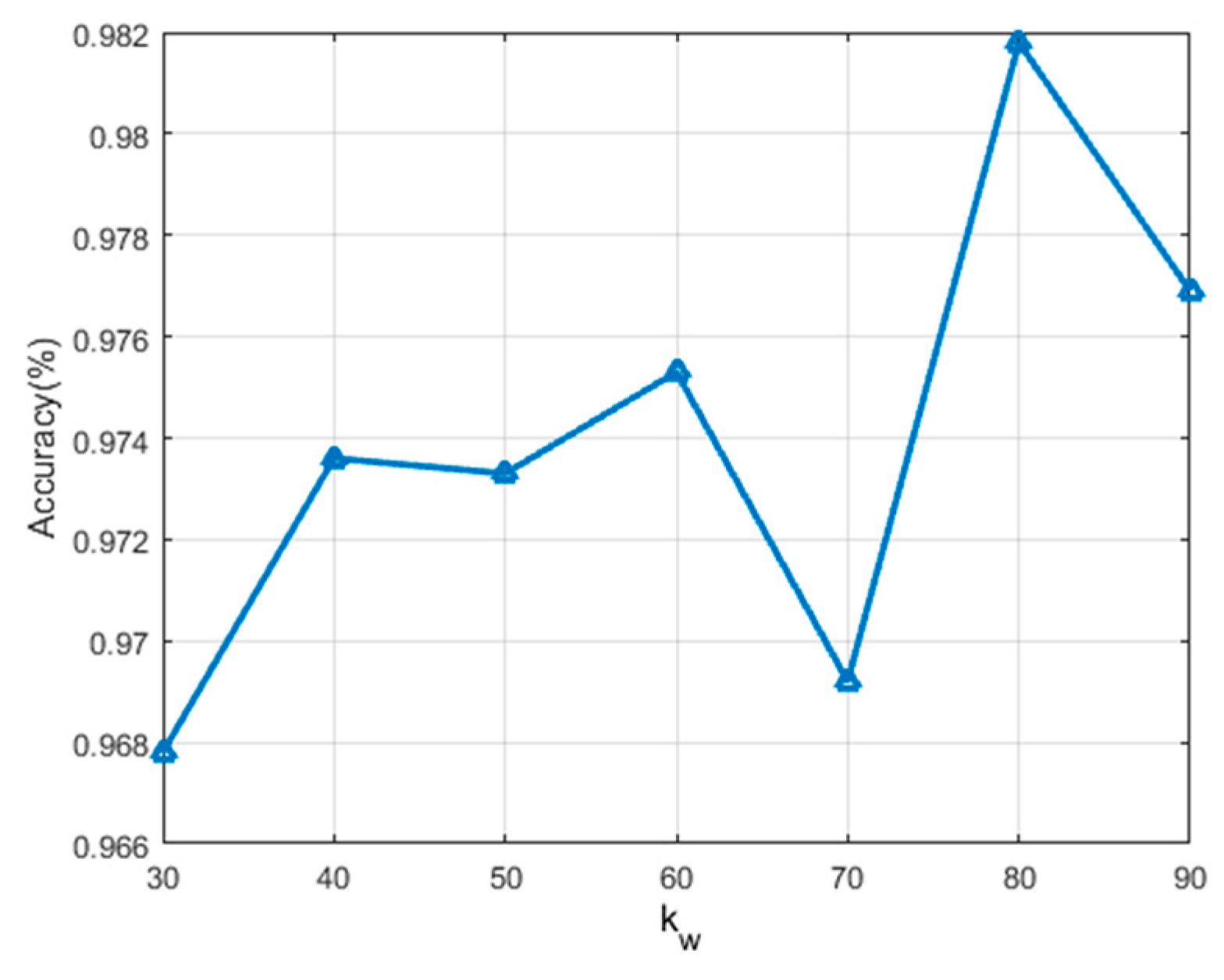
In addition, the effect of on the classification performance is discussed in the second group of experiments. is closely related to the robust feature representation that can effectively suppress the speckle noise in the neighborhood of each pixel. The experiment results are shown in Figure 6. It can be seen that the fold line has multiple peaks, and the highest accuracy is obtained when . We conclude that selecting a larger number of neighborhood pixels is more conducive to suppressing speckle noise and improving the classification performance. However, is also limited by the minimum size of superpixels, so it cannot increase infinitely.
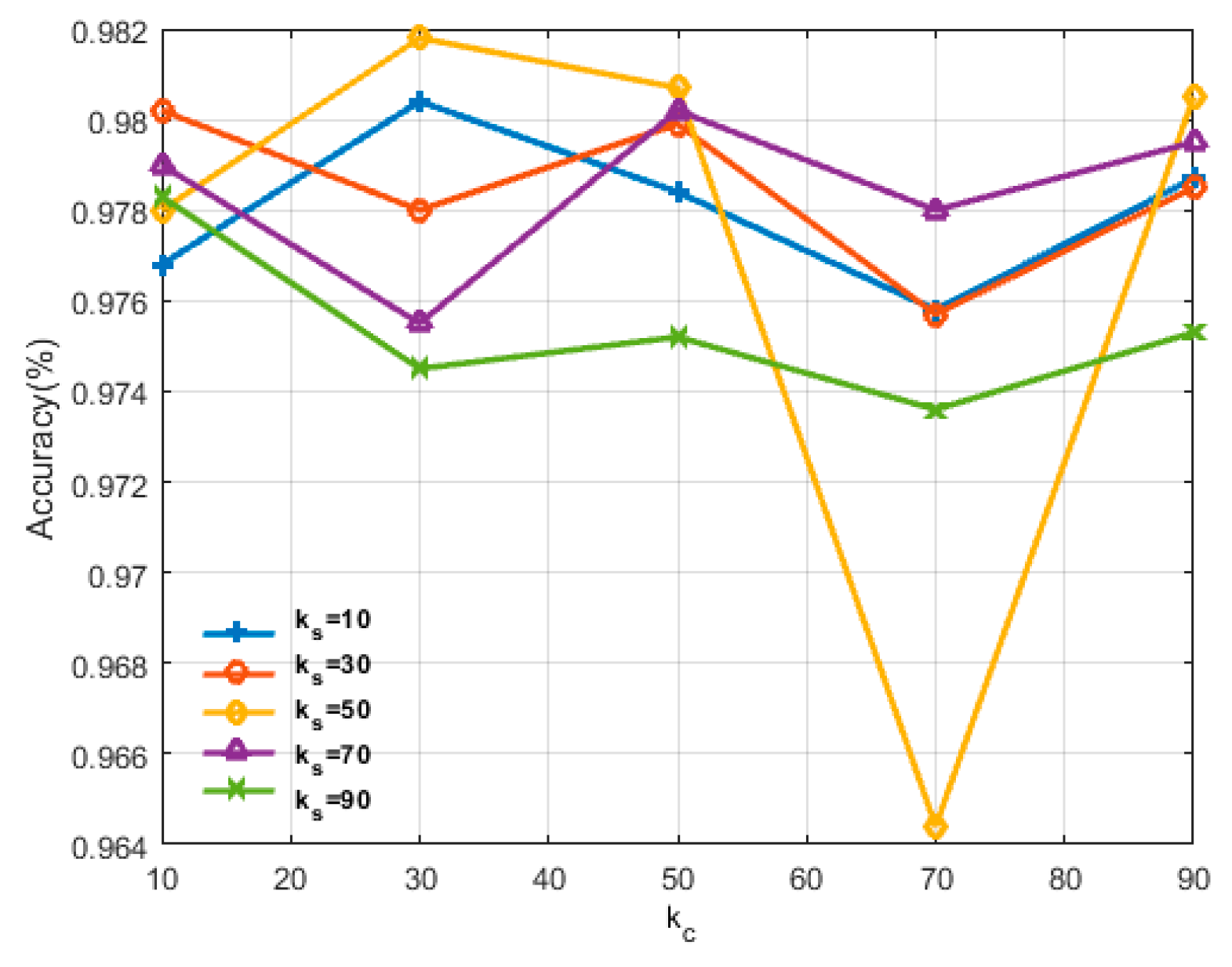
In the last group of experiments, we will discuss the effect of combinations of and used in the proposed semi-supervised unlabeled sample selection method. controls the maximum number of selected unlabeled samples per class in each iteration, and automatically controls the lower bound of the prediction confidence. We implemented the following experiments using a grid search. Each of the two parameters takes five values, which are 10, 30, 50, 70 and 90, respectively. Figure 7 shows the experiment results. The abscissa represents and the ordinate represents the classification accuracy.
Five fold lines that are marked with different shapes show effects of five different values of in combination with on the classification accuracy. Figure 7 shows that are the best choices for the proposed algorithm. It can also be inferred that two parameters mutually influence each other, as the variation in trends of all the lines is not always the same. On the one hand, the increment of and can increase the quantity and diversity of the selected samples, but on the other hand, it may import more uncertain information due to some inaccurately propagated labels. Thus, the values of and should be considered together and carefully selected.
To summarize, we over-segmented the Flevoland image into about 2000 homogeneous areas and used , by default for all experiments on the Flevoland dataset in this paper. With respect to the Oberpfaffenhofen data, we did the same parameter analysis as above. The number of superpixels n was set to 500 because there are larger homogeneous areas in the Oberpfaffenhofen image. The best choices of , and are 600, 30 and 80, respectively.
4.2. Performance Analysis
As mentioned in Section 3.2 and Section 3.3, the proposed algorithm obtains the best performance using the same sampling rate as the compared algorithms. We believe that this is due to the following reasons.
Wishart performs clustering according to the Wishart distance without any supervised information, which increases the possibility of misclassification. SVM is suitable for the classification of small samples, but it seems difficult for SVM to find the exact hyperplane when the number of categories increases. SSAE-LS is a typical supervised PolSAR classification algorithm that is greatly limited by the quantity and the quality of the training samples. It cannot recognize categories with few samples, such as buildings in the Flevoland dataset.
We also found that the two semi-supervised algorithms in this paper performed better, which may be because these algorithms can expand the training set by making full use of information from unlabeled samples. Nevertheless, there are obvious performance differences between them.
From our point of view, local and nonlocal similarity metrics used in SRDNN-MD may introduce some errors to unlabeled sample selection. Especially when regions of several categories with similar feature representations are close to each other, the edge of each category is affected by its neighboring categories. Pixels of two neighboring categories may locate in the same superpixel. The superpixel-restrained term introduced into the classifier in SRDNN-MD can enhance feature consistency within each superpixel, while it also brings confusing information of neighboring categories to the classifier. SRDNN-MD only has weak regional consistency between each category.
In contrast, the proposed algorithm selects unlabeled samples from the same superpixel that contains samples of great reliability and diversity so that the probability is greater than if they belong to the same category, which can reduce incorrect semi-supervised label propagations. This is helpful for the subsequent self-training process of the classifier. By innovatively proposing the semi-supervised unlabeled sample selection method based on superpixels, we effectively expand the training set and fully utilize the results of superpixel segmentation and the potential of semi-supervised learning. For these reasons, our method can obtain excellent classification results with a limited number of labeled training samples.
5. Conclusions
In this paper, we propose a novel semi-supervised PolSAR classification algorithm based on self-training and superpixels. We first construct a real feature vector that can effectively suppress the speckle noise-utilizing spatial weighting method based on superpixel segmentation. Then the proposed semi-supervised unlabeled sample selection method is used to propagate labels to the selected unlabeled samples and to expand the training set iteratively, making full use of the spatial information of neighborhood pixels in the same superpixel. Finally, an SSAE is self-trained to obtain classification results. It has been analyzed that the added new samples are of high reliability and high diversity, which are helpful for the following trainings. A large number of experiments and analyses on the Flevoland dataset verified the effectiveness and the superiority of the whole algorithm, and showed excellent performance with a limited number of labeled samples. Experiments on the Oberpfaffenhofent dataset confirmed that the proposed algorithm has good generalization capabilities.
One of the shortcomings is that the choice of parameters is a little complicated in the proposed algorithm. We will consider adding automatic parameter optimization to our framework in the future. Furthermore, although superpixels have great advantages in characterizing the spatial relationships of pixels, it is more efficient to utilize deep networks to simultaneously extract spatial features and deep features due to the popularity of deep learning, for example, convolution networks. Future research may use this idea to extend the basic framework to semi-supervised deep learning with a combination of characters of PolSAR, which may realize more robust feature representation.
Author Contributions
Methodology, R.X. and Y.C.; Data processing and experimental results analysis, R.X. and Y.L.; Oversight and suggestions, Y.L., L.J. and R.S.; Writing review and editing, Y.L., Y.C. and N.M.
Funding
This research was funded by the National Natural Science Foundation of China under Grant 61772399, Grant U1701267, Grant 61773304, Grant 61672405 and Grant 61772400, the Key Research and Development Plan of Innovation Chain of Industries in Shaanxi Province under Grant 2019ZDLGY09-05, the Program for Cheung Kong Scholars and Innovative Research Team in University Grant IRT_15R53, the Fund for Foreign Scholars in University Research and Teaching Programs (the 111 Project) Grant B07048, and the Technology Foundation for Selected Overseas Chinese Scholar in Shaanxi under Grant 2017021, Grant 2018021.
Acknowledgments
The author would like to show their gratitude to the editors and the anonymous reviewers for their insightful comments.
Conflicts of Interest
The authors declare no conflict of interest.
References
- Xie, Q.; Wang, J.; Liao, C.; Shang, J.; Lopez-Sanchez, J.M.; Fu, H.; Liu, X. On the Use of Neumann Decomposition for Crop Classification Using Multi-Temporal RADARSAT-2 Polarimetric SAR Data. Remote Sens. 2019, 11, 776. [Google Scholar] [CrossRef]
- Xi, Y.; Lang, H.; Tao, Y.; Huang, L.; Pei, Z. Four-Component Model-Based Decomposition for Ship Targets Using PolSAR Data. Remote Sens. 2017, 9, 621. [Google Scholar] [CrossRef]
- Omati, M.; Sahebi, M.R. Change Detection of Polarimetric SAR Images Based on the Integration of Improved Watershed and MRF Segmentation Approaches. IEEE J. Sel. Top. Appl. Earth Obs. Remote Sens. 2018, 11, 4170–4179. [Google Scholar] [CrossRef]
- Pottier, E. Dr. J.R. Huynen’s main contributions in the development of polarimetric radar techniques and how the ’Radar Targets Phenomenological Concept’ becomes a theory. Proc. SPIE 1748 Radar Polarim. 1993, 1748. [Google Scholar] [CrossRef]
- Cloude, S.R.; Pottier, E. An entropy based classification scheme for land applications of polarimetric SAR. IEEE Trans. Geosci. Remote Sens. 1997, 35, 68–78. [Google Scholar] [CrossRef]
- Freeman, A.; Durden, S.L. A three-component scattering model for polarimetric SAR data. IEEE Trans. Geosci. Remote Sens. 1998, 36, 963–973. [Google Scholar] [CrossRef] [Green Version]
- Yamaguchi, Y.; Sato, A.; Boerner, W.; Sato, R.; Yamada, H. Four-Component Scattering Power Decomposition with Rotation of Coherency Matrix. IEEE Trans. Geosci. Remote Sens. 2011, 49, 2251–2258. [Google Scholar] [CrossRef]
- Cloude, S.R.; Pottier, E. A review of target decomposition theorems in radar polarimetry. IEEE Trans. Geosci. Remote Sens. 1996, 34, 498–518. [Google Scholar] [CrossRef]
- Yamaguchi, Y.; Moriyama, T.; Ishido, M.; Yamada, H. Four-component scattering model for polarimetric SAR image decomposition. IEEE Trans. Geosci. Remote Sens. 2005, 43, 1699–1706. [Google Scholar] [CrossRef]
- Lee, J.S.; Grunes, M.R.; Kwok, R. Classification of multi-look polarimetric SAR imagery based on complex Wishart distribution. Int. J. Remote Sens. 1994, 15, 2299–2311. [Google Scholar] [CrossRef]
- Jong-Sen, L.; Grunes, M.R.; Ainsworth, T.L.; Li-Jen, D.; Schuler, D.L.; Cloude, S.R. Unsupervised classification using polarimetric decomposition and the complex Wishart classifier. IEEE Trans. Geosci. Remote Sens. 1999, 37, 2249–2258. [Google Scholar] [CrossRef]
- Liu, F.; Jiao, L.; Hou, B.; Yang, S. POLSAR Image Classification Based on Wishart DBN and Local Spatial Information. IEEE Trans. Geosci. Remote Sens. 2016, 54, 3292–3308. [Google Scholar] [CrossRef]
- Fukuda, S.; Hirosawa, H. Support vector machine classification of land cover: Application to polarimetric SAR data. In Proceedings of the IGARSS 2001. Scanning the Present and Resolving the Future. IEEE 2001 International Geoscience and Remote Sensing Symposium (Cat. No.01CH37217), Sydney, Australia, 9–13 July 2001; Volume 181, pp. 187–189. [Google Scholar]
- Du, P.; Samat, A.; Waske, B.; Liu, S.; Li, Z. Random Forest and Rotation Forest for fully polarized SAR image classification using polarimetric and spatial features. ISPRS-J. Photogramm. Remote Sens. 2015, 105, 38–53. [Google Scholar] [CrossRef]
- Hinton, G.E.; Osindero, S.; Teh, Y.W. A Fast Learning Alogorithm for Deep Belief Nets. Neural Comput. 2006, 18, 1527–1554. [Google Scholar] [CrossRef]
- Krizhevsky, A.; Sutskever, I.; Hinton, G.E. ImageNet classification with deep convolutional neural networks. Proc. Adv. Neural Inf. Process. Syst. 2017, 60, 84–90. [Google Scholar] [CrossRef]
- Hou, B.; Kou, H.; Jiao, L. Classification of Polarimetric SAR Images Using Multilayer Autoencoders and Superpixels. IEEE J. Sel. Top. Appl. Earth Obs. Remote Sens. 2016, 9, 3072–3081. [Google Scholar] [CrossRef]
- Xie, W.; Jiao, L.; Hou, B.; Ma, W.; Zhao, J.; Zhang, S.; Liu, F. POLSAR Image Classification via Wishart-AE Model or Wishart-CAE Model. IEEE J. Sel. Top. Appl. Earth Obs. Remote Sens. 2017, 10, 3604–3615. [Google Scholar] [CrossRef]
- Zhang, L.; Ma, W.; Zhang, D. Stacked Sparse Autoencoder in PolSAR Data Classification Using Local Spatial Information. IEEE Geosci. Remote Sens. Lett. 2016, 13, 1359–1363. [Google Scholar] [CrossRef]
- Chen, W.; Gou, S.; Wang, X.; Li, X.; Jiao, L. Classification of PolSAR Images Using Multilayer Autoencoders and a Self-Paced Learning Approach. Remote Sens. 2018, 10, 110. [Google Scholar] [CrossRef]
- Hänsch, R.; Hellwich, O. Semi-supervised learning for classification of polarimetric SAR-data. In Proceedings of the 2009 IEEE International Geoscience and Remote Sensing Symposium, Cape Town, South Africa, 12–17 July 2009; pp. III-987–III-990. [Google Scholar]
- Huo, L.; Tang, P.; Zhang, Z.; Tuia, D. Semisupervised Classification of Remote Sensing Images with Hierarchical Spatial Similarity. IEEE Geosci. Remote Sens. Lett. 2015, 12, 150–154. [Google Scholar] [CrossRef]
- Fang, B.; Li, Y.; Zhang, H.; Chan, J.C.W. Semi-Supervised Deep Learning Classification for Hyperspectral Image Based on Dual-Strategy Sample Selection. Remote Sens. 2018, 10, 574. [Google Scholar] [CrossRef]
- Jin, G.; Raich, R.; Miller, D.J. A generative semi-supervised model for multi-view learning when some views are label-free. In Proceedings of the 2013 IEEE International Conference on Acoustics, Speech and Signal Processing, Vancouver, BC, Canada, 26–31 May 2013; pp. 3302–3306. [Google Scholar]
- Geng, J.; Ma, X.; Fan, J.; Wang, H. Semisupervised Classification of Polarimetric SAR Image via Superpixel Restrained Deep Neural Network. IEEE Geosci. Remote Sens. Lett. 2018, 15, 122–126. [Google Scholar] [CrossRef]
- Hua, W.; Wang, S.; Liu, H.; Liu, K.; Guo, Y.; Jiao, L. Semisupervised PolSAR Image Classification Based on Improved Cotraining. IEEE J. Sel. Top. Appl. Earth Obs. Remote Sens. 2017, 10, 4971–4986. [Google Scholar] [CrossRef]
- Yang, L.; Yang, S.; Jin, P.; Zhang, R. Semi-Supervised Hyperspectral Image Classification Using Spatio-Spectral Laplacian Support Vector Machine. IEEE Geosci. Remote Sens. Lett. 2014, 11, 651–655. [Google Scholar] [CrossRef]
- Liu, H.; Wang, Y.; Yang, S.; Wang, S.; Feng, J.; Jiao, L. Large Polarimetric SAR Data Semi-Supervised Classification with Spatial-Anchor Graph. IEEE J. Sel. Top. Appl. Earth Obs. Remote Sens. 2016, 9, 1439–1458. [Google Scholar] [CrossRef]
- Uhlmann, S.; Kiranyaz, S.; Gabbouj, M. Semi-Supervised Learning for Ill-Posed Polarimetric SAR Classification. Remote Sens. 2014, 6, 4801–4830. [Google Scholar] [CrossRef] [Green Version]
- Achanta, R.; Shaji, A.; Smith, K.; Lucchi, A.; Fua, P.; Süsstrunk, S. SLIC Superpixels Compared to State-of-the-Art Superpixel Methods. IEEE Trans. Pattern Anal. Mach. Intell. 2012, 34, 2274–2282. [Google Scholar] [CrossRef]
- Ren, M. Learning a classification model for segmentation. In Proceedings of the Ninth IEEE International Conference on Computer Vision, Nice, France, 13–16 October 2003; Volume 11, pp. 10–17. [Google Scholar]
- Xu, Q.; Chen, Q.; Yang, S.; Liu, X. Superpixel-Based Classification Using K Distribution and Spatial Context for Polarimetric SAR Images. Remote Sens. 2016, 8, 619. [Google Scholar] [CrossRef]
- Wang, W.; Xiang, D.; Ban, Y.; Zhang, J.; Wan, J. Superpixel-Based Segmentation of Polarimetric SAR Images through Two-Stage Merging. Remote Sens. 2019, 11, 402. [Google Scholar] [CrossRef]
- Jianbo, S.; Malik, J. Normalized cuts and image segmentation. In Proceedings of the IEEE Computer Society Conference on Computer Vision and Pattern Recognition, San Juan, PR, USA, 17–19 June 1997; pp. 731–737. [Google Scholar]
- Comaniciu, D.; Meer, P. Mean shift: A robust approach toward feature space analysis. IEEE Trans. Pattern Anal. Mach. Intell. 2002, 24, 603–619. [Google Scholar] [CrossRef]
- Levinshtein, A.; Stere, A.; Kutulakos, K.N.; Fleet, D.J.; Dickinson, S.J.; Siddiqi, K. TurboPixels: Fast Superpixels Using Geometric Flows. IEEE Trans. Pattern Anal. Mach. Intell. 2009, 31, 2290–2297. [Google Scholar] [CrossRef]
Figure 1.
The flow of semi-supervised unlabeled sample selection. Take five superpixels in a neighborhood for example. Red squares indicate labeled training samples and black squares indicate unlabeled candidate samples, respectively.
Figure 1.
The flow of semi-supervised unlabeled sample selection. Take five superpixels in a neighborhood for example. Red squares indicate labeled training samples and black squares indicate unlabeled candidate samples, respectively.

Figure 2.
The structure of an SAE. x, h and y are the input data, the hidden data and the reconstruction of input data, respectively.
Figure 2.
The structure of an SAE. x, h and y are the input data, the hidden data and the reconstruction of input data, respectively.

Figure 3.
Results of different methods on Flevoland. (a) Pauli RGB image. (b) Ground truth. (c) Superpixel-based segmentation results (n = 2000). (d) Wishart. (e) SVM. (f) SSAE-LS. (g) SRDNN-MD. (h) Proposed. (i) Color code.
Figure 3.
Results of different methods on Flevoland. (a) Pauli RGB image. (b) Ground truth. (c) Superpixel-based segmentation results (n = 2000). (d) Wishart. (e) SVM. (f) SSAE-LS. (g) SRDNN-MD. (h) Proposed. (i) Color code.

Figure 4.
Results of different methods on Oberpfaffenhofen. (a) Pauli RGB image. (b) Ground truth. (c) Superpixel-based segmentation results (n = 500). (d) Wishart. (e) SVM. (f) SSAE-LS. (g) SRDNN-MD. (h) Proposed. (i) Color code.
Figure 4.
Results of different methods on Oberpfaffenhofen. (a) Pauli RGB image. (b) Ground truth. (c) Superpixel-based segmentation results (n = 500). (d) Wishart. (e) SVM. (f) SSAE-LS. (g) SRDNN-MD. (h) Proposed. (i) Color code.

Figure 5.
Effect of the number of superpixels n on the classification accuracy.

Figure 6.
Effect of on the classification accuracy.

Figure 7.
Effect of and on the classification accuracy.


Table 1.
Number of training samples and ground truth samples on Flevoland data.
| Training Samples | Ground Truth | |
|---|---|---|
| Stembeans | 63 | 6338 |
| Rapeseed | 139 | 13863 |
| Bare Soil | 51 | 5109 |
| Potatoes | 162 | 16156 |
| Beet | 100 | 10033 |
| Wheat2 | 112 | 11159 |
| Peas | 96 | 9582 |
| Wheat3 | 222 | 22241 |
| Lucerne | 102 | 10181 |
| Barley | 76 | 7595 |
| Wheat | 164 | 16386 |
| Grasses | 71 | 7058 |
| Forest | 180 | 18044 |
| Water | 132 | 13232 |
| Buildings | 7 | 735 |
| Total | 1677 | 167712 |
Table 2.
Classification accuracy (%) comparisons on Flevoland data.
| Unsupervised | Supervised | Semi-supervised | |||
|---|---|---|---|---|---|
| Class | Wishart [10] | SVM [13] | SSAE-LS [19] | SRDNN-MD [25] | Proposed |
| Stembeans | 94.88 | 85.80 | 97.71 | 97.08 | 98.33 |
| Rapeseed | 72.05 | 86.16 | 80.47 | 91.81 | 97.57 |
| Bare Soil | 5.18 | 82.48 | 82.01 | 93.92 | 98.66 |
| Potatoes | 87.28 | 80.99 | 89.51 | 94.19 | 98.72 |
| Beet | 92.77 | 88.5 | 92.91 | 92.38 | 99.4 |
| Wheat2 | 81.89 | 74.38 | 92.65 | 89.65 | 98.1 |
| Peas | 96.90 | 90.3 | 96.88 | 94.52 | 98.97 |
| Wheat3 | 89.35 | 90.76 | 96.06 | 97.60 | 99 |
| Lucerne | 92.58 | 88.73 | 97.39 | 95.55 | 98.72 |
| Barley | 94.21 | 96.45 | 93.19 | 97.54 | 97.93 |
| Wheat | 85.13 | 84.88 | 91.83 | 95.52 | 98.08 |
| Grasses | 72.52 | 47.76 | 63.95 | 87.26 | 91.5 |
| Forest | 88.47 | 77.16 | 91.34 | 97.31 | 99.71 |
| Water | 47.96 | 89.97 | 86.48 | 99.53 | 96.41 |
| Buildings | 83.93 | 91.48 | 39.97 | 81.74 | 99.31 |
| OA | 81.42 | 83.98 | 90.08 | 94.66 | 98.18 |
| AA | 81.42 | 83.72 | 86.16 | 93.71 | 98.03 |
| Kappa | 0.7979 | 0.8254 | 0.8919 | 0.9418 | 0.9802 |
| Used Labels | 1% | 1% | 1% | 1% | 1% |
Table 3.
Number of training samples and ground truth samples on the Oberpfaffenhofen data.
| Training Samples | Ground Truth | |
|---|---|---|
| Built-up Area | 1000 | 320688 |
| Wood Land | 1000 | 270858 |
| Open Area | 1000 | 747314 |
| Total | 3000 | 1338860 |
Table 4.
Classification accuracy (%) comparisons on Oberpfaffenhofen.
| Unsupervised | Supervised | Semi-supervised | |||
|---|---|---|---|---|---|
| Class | Wishart [10] | SVM [13] | SSAE-LS [19] | SRDNN-MD [25] | Proposed |
| Built-up Area | 10.41 | 67.17 | 74.76 | 89.90 | 87.2 |
| Wood Land | 95.67 | 94.21 | 95.42 | 94.53 | 95.52 |
| Open Area | 93.94 | 84.55 | 87.41 | 93.92 | 97.51 |
| OA | 74.3 | 85.69 | 88.79 | 93.09 | 94.3 |
| AA | 74.3 | 81.98 | 85.86 | 92.78 | 92.87 |
| Kappa | 0.5577 | 0.7548 | 0.8077 | 0.8842 | 0.9018 |
| Used Labels | 1000 | 1000 | 1000 | 1000 | 1000 |
© 2019 by the authors. Licensee MDPI, Basel, Switzerland. This article is an open access article distributed under the terms and conditions of the Creative Commons Attribution (CC BY) license (http://creativecommons.org/licenses/by/4.0/).
Share and Cite
MDPI and ACS Style
Li, Y.; Xing, R.; Jiao, L.; Chen, Y.; Chai, Y.; Marturi, N.; Shang, R. Semi-Supervised PolSAR Image Classification Based on Self-Training and Superpixels. Remote Sens. 2019, 11, 1933. https://doi.org/10.3390/rs11161933
AMA Style
Li Y, Xing R, Jiao L, Chen Y, Chai Y, Marturi N, Shang R. Semi-Supervised PolSAR Image Classification Based on Self-Training and Superpixels. Remote Sensing. 2019; 11(16):1933. https://doi.org/10.3390/rs11161933
Chicago/Turabian StyleLi, Yangyang, Ruoting Xing, Licheng Jiao, Yanqiao Chen, Yingte Chai, Naresh Marturi, and Ronghua Shang. 2019. "Semi-Supervised PolSAR Image Classification Based on Self-Training and Superpixels" Remote Sensing 11, no. 16: 1933. https://doi.org/10.3390/rs11161933
Note that from the first issue of 2016, this journal uses article numbers instead of page numbers. See further details here.