Hydrological Response of Dry Afromontane Forest to Changes in Land Use and Land Cover in Northern Ethiopia


1
Department of Environmental Science and Ecological Engineering, Korea University, Seoul 02841, Korea
2
Mekelle Environment and Forestry Research, Ethiopian Environment and Forestry Research Institute, Addis Ababa 1000, Ethiopia
3
Institute of Climate and Society, Mekelle University, Mek’ele 231, Ethiopia
*
Author to whom correspondence should be addressed.
Remote Sens. 2019, 11(16), 1905; https://doi.org/10.3390/rs11161905
Submission received: 21 June 2019
/
Revised: 6 August 2019
/
Accepted: 12 August 2019
/
Published: 15 August 2019
(This article belongs to the Special Issue Selected Papers from the "2019 International Symposium on Remote Sensing")
Abstract
:This study analyzes the impact of land use/land cover (LULC) changes on the hydrology of the dry Afromontane forest landscape in northern Ethiopia. Landsat satellite images of thematic mapper (TM) (1986), TM (2001), and Operational Land Imager (OLI) (2018) were employed to assess LULC. All of the images were classified while using the maximum likelihood image classification technique, and the changes were assessed by post-classification comparison. Seven LULC classes were defined with an overall accuracy 83–90% and a Kappa coefficient of 0.82–0.92. The classification result for 1986 revealed dominance of shrublands (48.5%), followed by cultivated land (42%). Between 1986 and 2018, cultivated land became the dominant (39.6%) LULC type, accompanied by a decrease in shrubland to 32.2%, as well as increases in forestland (from 4.8% to 21.4%) and bare land (from 0% to 0.96%). The soil conservation systems curve number model (SCS-CN) was consequently employed to simulate forest hydrological response to climatic variations and land-cover changes during three selected years. The observed changes in direct surface runoff, the runoff coefficient, and storage capacity of the soil were partially linked to the changes in LULC that were associated with expanding bare land and built-up areas. This change in land use aggravates the runoff potential of the study area by 31.6 mm per year on average. Runoff coefficients ranged from 25.3% to 47.2% with varied storm rainfall intensities of 26.1–45.4 mm/ha. The temporal variability of climate change and potential evapotranspiration increased by 1% during 1981–2018. The observed rainfall and modelled runoff showed a strong positive correlation (R2 = 0.78; p < 0.001). Regression analysis between runoff and rainfall intensity indicates their high and significant correlation (R2 = 0.89; p < 0.0001). Changes were also common along the slope gradient and agro-ecological zones at varying proportions. The observed changes in land degradation and surface runoff are highly linked to the change in LULC. Further study is suggested on climate scenario-based modeling of hydrological processes that are related to land use changes to understand the hydrological variability of the dry Afromontane forest ecosystems.
1. Introduction
Forests provide multitudes of essential ecosystem services [1], such as soil nutrient cycling, build-up of organic matter, and water retention. Forest biodiversity losses may seriously jeopardize the functioning of forest ecosystems, and consequently the ability of forests to provide ecosystem services [2]. In the past few decades, tropical landscapes were facing critical environmental challenges [3,4] that were related to rapid land use and land cover (LULC) change, such as massive deforestation and land conversion. The Forest Resource Assessment (FRA) that was completed by Food and Agriculture organization (FAO) in 2005 and preliminary results of FRA 2015 [5] indicate that, on a global scale, the total forest area continues to decrease by 3.1%, which is about 0.6% per year from 2000 to 2005 [3,6] and 3.3% per year from 2010 to 2015 [5]. Deforestation continues at the highest rates across the tropics, and FRA estimates for 1990–2005 suggest annual rates of deforestation at 0.9% in South and Southeast Asia, 1.2% in Central America, 0.45% in South America, and 0.62% in Africa [3]. This means that, on average, each year from 1990 to 2015, an area of 4128–3999 million ha, which is above 3.1% of the tropical forest, was lost [3]. The change in land use is considered to contribute to 20% of global greenhouse gas emissions [7,8]. In particular, forest degradation in sub-Saharan Africa is the main source of land-based emissions [9,10].
According to Pielke [11], LULC changes influence climatic and weather conditions, ranging from local to global levels. Biophysical factors, such as topography, soil type, and seasonal rainfall, as well as demographic, political, economic, and social factors combined together lead to large changes in land use in East Africa, and these trends are expected to continue into the future [3,5]. Similarly to the above studies, Ethiopia is experiencing significant LULC dynamics, such as land conversion from natural vegetation to agricultural and urban areas [12,13,14,15]. The problem is more severe in the highlands, which account for 44% of the country’s landmass and they have been cultivated for centuries [16,17,18,19,20,21,22,23,24]. Land use dynamics during 1975–2016 in India reported that agricultural land increased by 18%, whereas forest land and rangeland decreased by 7% and 10%, respectively [25]. Specifically, in the northern highlands of Ethiopia, increasing land degradation due to the loss of the remnant forests, which are found in sacred and inaccessible places [26] and cultivation of the sloppy lands [19] aggravates runoff and reduces the infiltration capacity of the area. The change in land use is considered to contribute to 20% of global greenhouse gases emissions [7,8]. Land cover change is defined as the change in land cover and its associated properties over time [27,28]. LULC change constitutes one of the fundamental environmental problems in Ethiopia [29,30,31,32]. For example, a study in the Afar region of northern Ethiopia reported that the invasion of Prosopis juliflora increased at annual rates of 31,127 ha, while grassland and bush-shrub-woodland declined at 19,312 ha and 10,543 ha, respectively [31].
The findings of Palma et al. [33] also indicate that land use changes have the potential to affect landscape hydrology, thereby aggravating runoff. The hydrological response is a combined indicator of the watershed condition and significant changes in LULC, reflecting the overall health and function of a semi-arid watershed [34]. Other studies [18,19,35] showed that the simulated impact of climate change on hydrological processes significantly varies, depending on the climate model and emission scenarios, in addition to geographical variation [36,37].
The alteration of tropical landscapes, primarily the conversion of natural forests to agriculture or pasture [11], directly influence the hydrology of the landscape, and the relative impacts of different potential drivers of these extreme events on the hydrological cycle are still debated. External factors include meteorological variations, which result in periods of increased extreme events or climatic non-stationarity. The internal factors include abstractions and discharges in the river, land use change, and modification of the river flow channel.
LULC changes significantly affected regional hydrology [38,39,40,41], and consequently the delivery of ecosystem services [42,43] and climate processes. The impact of LULC on environmental processes is not universal and it depends on the local context of a particular region [44]. Gebremicael et al. [45] revealed that more than 72% of the northern Ethiopian landscape was significantly altered during 1972–2014 in the head water of the Tekeze-Atbara Basin. A study by Guzha et al. [46] in East Africa has shown that forest cover loss increased the annual discharges by 16% and surface runoff by 45%. Bewket and Sterk [47] showed that changes in land management practices are the main factors of variability in water availability in Ethiopia. In particular, Gebresamuel et al. [13] have reported that the changes in LULC decreased the water-storage capacity of soils by 1.63 mm/y at Gum Selassa and 1.09 mm/y at Maileba of northern Ethiopia, with a corresponding increase in the surface runoff by 2.7 mm/y and 2.3 mm/y, respectively. The other concern is the effect of global climate change, mainly relating to the patterns and amounts of rainfall in the upper catchment areas, which directly affect runoff patterns [48]. Significant variation in evapotranspiration occurs due to LULC accompanied with the leaf area index change [49]. Generally, land use change can lead to a significant change in groundwater recharge and base flow [50], flood frequency and interval [51], peak runoff [52], and total suspended sediment and nutrient concentration [53]. Land restoration has been successful in improving the vegetation cover, and consequently the hydrological processes of degraded landscapes [47]. For example, the restoration of steep hillsides enhances the initial retention capacity of the soil, thereby limiting the runoff curve number [13,35,54,55,56].
Physically based distributed hydrological models have become important for the understanding of fundamental physical processes that underlie the hydrological cycle and developing scenario-based solutions to adverse changes in forest hydrology at different spatial scales [57]. The development of satellite remote sensing is important for modelling capabilities to evaluate and predict the hydrological consequences of land-use change at multiple scales. For example, the conceptual and empirical foundations of the soil conservation service curve number (SCS-CN) method have been applied to a wide range of catchments across the world to assess the effects of land cover change on surface runoff [27,58,59,60,61,62,63,64]. The runoff coefficient forecasts direct surface runoff volume for a given rainfall event and estimates the volumes and peak rates of surface runoff in catchments [58]. The rainfall-runoff relations within a watershed are primarily driven by the relationship of factors, such as climate, land cover, and soil [36,37,38,39]. The SCS-CN model expresses runoff volume as a function of rainfall volume, hydrologic storage, and initial abstraction [65]. The CN value depends on the land surface features and hydrological soil conditions of the entire watershed.
The original SCS-CN method computes direct runoff by only considering the available rainfall on the current day without taking the effect of the moisture available prior to the storm into consideration. In contrast, the curve numbers are sensitive to antecedent conditions [66]. The existing SCS-CN method does not contain any expression for time, and it ignores the impact of rainfall intensity and its temporal distribution. There is no explicit provision for spatial scale effects either. The other demerits of the existing SCS-CN method are the absence of clear guidance on how to vary the antecedent moisture conditions and the fixing of initial abstraction ratio 0.2, preempting a regionalization that is based on geological and climatic settings [67].
Research on runoff patterns in response to land cover dynamics allows for the assessment of sustainability of land use systems in dry areas, as the runoff reflects the ecological state of the entire watershed. Modeling allows evaluating long-term hydrological consequences of LULC change in dry Afromontane forests and provides quantitative information for land use planning and water resources management. However, developing countries face difficulties in different aspects of hydrological modeling research, such as the availability of continuously measured data. Therefore, combining the remote sensing technique, point-based meteorology data, and hydrological modeling can help in understanding and evaluating the existing LULC conditions of the undulating and mountainous dry Afromontane forests. This information can also be employed to forecast the likely effects of any potential changes in land cover on water resource systems. Hence, such a study has practical relevance for devising strategies and policies for sustainable land and water use. No studies have been published to date combining the remote sensing technique and evapotranspiration and modeled surface hydrology information in forest areas of the dry Afromontane forest in northern Ethiopia, to the best of our knowledge.
The dry Afromontane forest landscape in northern Ethiopia is characterized by prolonged dry seasons, under conditions of low humidity, high air temperatures, and drying up of seasonal rivers and streams due to natural and human-induced factors [55,68]. Some studies on streamflow patterns with respect to land cover dynamics enabled the assessment of sustainability of land use systems, because stream flows are reflections of the ecological state of the entire watershed [47,55,69,70]. However, little is known regarding land use dynamics with respect to catchment hydrology [47,69], soil degradation [71], soil properties, and surface runoff [13] in Ethiopia. This study integrated high-resolution temporal LULC maps that were derived from satellite imagery with hydrological modeling to evaluate long-term hydrological consequences of LULC change in dry Afromontane forests and provide quantitative information for land use planning and water resource management. In particular, we aimed to adapt the conventional SCS-CN model by incorporating the variation of daily curve numbers with respect to the variability of antecedent rainfall, potential evapotranspiration (PET) with integrated LULC change images, and grid-based hydrological soil texture classification groups (HSG). The modified SCS-CN-based models provide a hydrologically sound procedure for a more accurate representation of the catchment behavior through analysis of the hydrological response of LULC changes, as indicated by their impact on the PET and runoff coefficient in the dry Afromontane forest landscape of northern Ethiopia.
2. Materials and Methods
2.1. Study Area Description
Topographically, northern Ethiopia is characterized by an undulating to steep terrain that is frequently divided by stream incisions. Thus the northern Ethiopian climate exhibits extreme climatic variations within short distances, from very dry tropical to sub-humid and subtropical to highly-moist tropical climates. The average annual rainfall varies from 200 mm in the arid lowlands to over 2200 mm in parts of the southwestern highlands. The mean annual temperatures vary from above 35 °C in the lowlands to less than 15 °C in the highland areas.
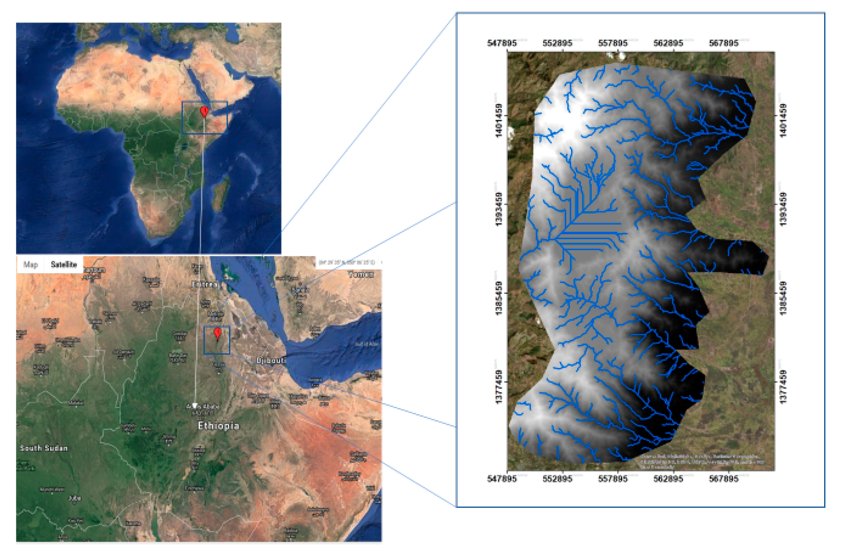
The estimated area of Ethiopian drylands is over 75 million ha, which accounts for about 66–72% of the total area of the country [72,73,74]. The study area lies between 39°10′E–40°02′34.08″ E and 12°53′29.76″N–12°′2.88″N (Figure 1). The study was carried out in two neighboring fragmented state forests of Hugumburda Grat Kahisu and the Tabotat natural forest areas of northern Ethiopia. This priority state forest has a minimum mean annual temperature range between 6.3 °C and 20.6 °C. The maximum mean annual temperature ranges from 15.1 °C to 29.7 °C. The mean annual rainfall ranges between 350 mm to more than 1000 mm (Table 1) in the lowland of Raya Azebo and the highlands of Korem districts, respectively. Mixed farming systems dominate the local agricultural activity. The dominant food crops grown are Zea mays, Sorghum bicolor, Triticum durum, Eragrostis tef, Hordeum vulgare, Pisum sativum, and Cicer arietinum. High-value tree crops, such as Mangifera indica, Persea americana, Carica papaya, and Psidium guajava, in the lowland and Malus domestica in the highlands of the Endamohoni and Offla districts are produced in large quantities. Cattle, sheep, goats, equines (donkey, horse, mule), and camel are the major livestock species reared.
The indigenous dry Afromontane forests of Northern Ethiopia are dominantly characterized by Juniperu sprocera, Olea europaea subsp. cuspidata, Maytenus arbutifolia, Maytenus senegalensis, Dodonaea angustifolia, Hagenia abyssinica, Bersama abyssinica, Acacia abyssinica, and Podocarpus falcatus in the highlands and midlands, while various Acacia species dominate the lowlands.
2.2. Methodology
2.2.1. Remote Sensing Data Collection and Processing
Satellite images for the years 1986, 2001, and 2018 were acquired to analyze the spatio-temporal patterns of the LULC of the fragmented state forests of Hugumburda Grat Kahisu and Tabotat natural forest areas. Landsat 5-Thematic mapper (TM) and Landsat-8 Operational Land Imager (OLI) images for the selected years were obtained from the US Geological Survey (USGS) Centre for Earth Resources Observation and Science (EROS), found in http://glovis.usgs.gov/. A brief description of the collected satellite images, including satellite and sensors used, resolution, acquisition date, 168/051 path/row of each images for each period is summarized in Table 2. Data acquisition was entirely conducted during the dry season to avoid phenological effects and ensure cloud-free images.
Remotely sensed data were pre-processed while using ERDAS Imagine 2015 software. Image rectification, restoration, enhancement, classification, and accuracy assessment were conducted using this software. ArcGIS 10.6 and ENVI 5.3 software were employed for managing, analyzing, combining, and mapping spatial data.
The analysis was performed on freely available satellite imagery products from Landsat 5 and Landsat 8 OLI at 30 m resolution. Spatial and temporal data from remote sensing integrated to World Geographic Coordinate System (GCS WGS 1984) was used to illustrate the Ethiopian administrative boundaries. The study aimed to determine the hydrological response of the fragmented state forests of northern Ethiopia to the dynamic LULC. Satellite images for a dry month have been considered for analysis to avoid seasonal factors, such as phenological effects. LULC information was then extracted while using the supervised maximum likelihood classification method by collecting 350 ground control points (GCP) for training signature generation and another 350 GCPs for accuracy assessment. Soil data were derived from the initial soil map, which are available online from the International Soil Reference and Information Centre (ISRIC) SoilsGrid250 [75] and modified based on the study area characteristics.
2.2.2. Data Acquisition and Processing
Stow [76] stated that accurate per-pixel registration of multi-temporal remote sensing data is essential for change detection analysis, since possible registration errors might be interpreted as LULC changes, leading to an overestimation of the actual change. In this study, image pre-processing (geometric and atmospheric corrections and topographic and temporal normalizations) was performed for all LULC maps. All of the satellite images and digitized ancillary paper maps were georeferenced to a common coordinate system while using the topographic map at 1: 50,000 scale, the Universal Transverse Mercator (UTM) map projection (Zone 37), and WGS 84 datum in ArcGIS 10.6 and Erdas Imagine 2015.
The digital elevation model (DEM) of the Hugumburda Grat Kahisu state forest was downloaded from the SRTM (http://gdem.erssdac.jspacesystems.or.jp/) with a resolution of 30 m. The downloaded tiles were merged using mosaic capabilities of Arc GIS 10.6 to form a single DEM of the study area since 30 by 30 DEM resolution of SRTM is usually stored as tiled datasets. DEM was used to simulate the stream network and delineate the watershed into a series of interconnected sub-basins. The soil map, available online from ISRIC SoilsGrid250 [75], was modified based on the study area characteristics that were provided by the National Meteorological Agency (NMA). The climatic data, such as daily precipitation, as well as minimum and maximum temperature, were collected from Korem meteorology stations located within the state forest.
Climate data were provided by the National Meteorological Agency (NMA). The temporal climatic data used for this study were daily precipitation and daily minimum and maximum temperature collected at Korem and Hashengie meteorology stations located within the state forests.
2.2.3. Land Cover Dynamics
Supervised classification was used to classify the LULC change of the areas in the northern Ethiopian mountainous ecotones. A total of seven LULC classes, namely shrubland, grassland, bare land, forest, cultivated land, water bodies, and built-up areas were specified. All seven classes were identified in all the images for the selected study years in a consistent manner. For training points, more than 250 sample plots per LULC class were randomly assigned. Simple random sampling was employed to generate reference data while using high resolution Google Earth images and expert knowledge.
Accuracy assessment was conducted on the resulting classified imagery. This process includes generating a set of points in the classified imagery and comparing them with actual points on the ground through field work using GPS point-based sampling. GPS points for each land cover class were collected at the field level to complete the accuracy assessment. The LULC classification assigned to each pixel was then compared with the same location on the reference sources to determine whether the classification result was accurate. Field visits were conducted from December 2018 to February 2019 for collecting data on the existing land use type. A transect line was laid across the gradient with a distance of 2 2 km2 between the plot and randomly among the transect lines. More than 750 sample plots were gathered while using GPS with a plot size of 30 30 m2 by assuming the pixel size of the Landsat data for the undulating mountainous areas of HGK state forest in northern Ethiopia. These ground truthing data were used to train the maximum likelihood classifier (MLC) classifier. This gradient classification method allocates all of the pixels in a dataset to clusters that are defined by the mean value of the training datasets. The actual classification was carried out after the training data had been established (half of the sample data) and the MLC algorithm that was selected for the classification. MLC uses a parametric statistical approach to prepare the probability density distribution functions for each individual class [11,77]. Hence, MLC considers not only the cluster center, but also its shape, size, and orientation [78,79]. The assumption of most MLCs is that the statistics of the clusters have a ‘normal’ (Gaussian) distribution. The data that were collected during ground truthing were stored in Excel and converted to shape files using Arc GIS 10.6 software, after which they were used for LULC classification, analysis, and accuracy assessments in ERDAS 2015 version software.
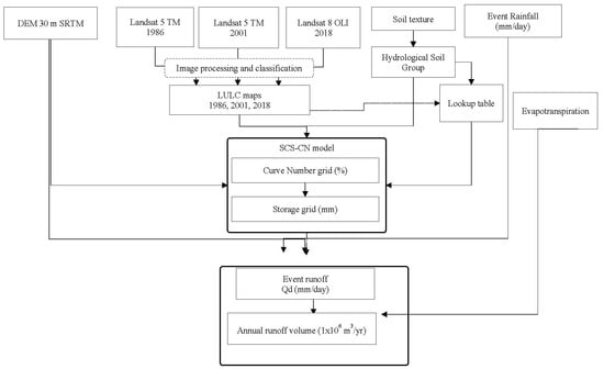
Figure 2 illustrates the overall conceptual frame work we followed to assess and estimate the annual runoff using SCS-CN curve number model.
2.3. Estimation for Runoff Response
Long-term hydro-meteorological data is required to understand the hydrological response of a catchment. However, hydrological data is often lacking in the developing world, and particularly in the study area in Hugumburda Grat Kahisu and Tabotat fragmented natural forests of northern Ethiopia. In the absence of sufficient hydrological data, empirical models, such as SCS-CN (USDA, 2004b, 2004a), are used as a substitute [13,54,80]. The SCS-CN method is based on the water balance equation and two fundamental hypotheses. The first hypothesis equates the ratio of actual amount of direct surface runoff Q to the total rainfall P (or maximum potential surface runoff) to the ratio of actual infiltration F to the amount of the potential maximum retention S. The second hypothesis relates the initial abstraction Ia to the potential maximum retention S. This study applied the same method to estimate the direct runoff response. The model quantifies the effect of changes in rainfall and land cover on the hydrological response of the dry Afromontane forest-based catchments.
Although direct runoff estimation is usually carried out at two abstraction ratios i.e., 0.05 and 0.2, studies on the highlands of northern Ethiopia [54,80,81] recommended λ = 0.05 as an optimum initial abstraction ratio that is based on least squares fitting for most experimental plots. The model’s statistical algorithm can be written as:
Where Qd is the estimated runoff (mm), P is the measured daily rainfall (mm), Ia is the initial abstraction (mm), λ is the initial abstraction ratio, and S is the maximum water retention parameter (mm) determined from the weighted CN value. S is related to the dimensionless runoff curve number (CN), which is given by the equation below.
Here, S is the maximum water retention parameter (mm) and CN is the weighted curve number that is calculated while using the equation below, based on the storm-event method [82], which is a data-derived value that varies according to the rainfall [58,81].
Here, A1, A2, A3, …, and An are the areas of hydrological groups that a given land cover falls into, and CN1, CN2, CN3, …, and CNn are the corresponding curve numbers.
2.4. Hydrologic Soil Group (HSG) Classification
The HSG of the study area was adopted from the classification that was employed in the USA developed by Cronshey [83], which is based on the infiltration rate controlled by the soil profile (Table 3). Technical Release 55 (TR-55) of urban hydrology for small watersheds presents the hydrologic soil group type according to the surface soil texture. Sand, loamy sand, and sandy loam belong to type A of HSG, silt loam and loam belong to type B of HSG, sandy clay loam belongs to type C of HSG, and clay loam, silty clay loam, sandy clay, silty clay, and clay belong to type D of HSG (Table 4).
2.5. Data Analysis
Model input data of historical daily rainfall and temperature data of 1981–2018 were used to generate climatological data sets for input into the model. The mass curve method [85,86] was employed to verify the consistency of rainfall values. As indicated by Garg [86], all input data were rendered into a grid format, and the isohyetal method was used to interpolate the areal rainfall. Table 1 summarizes the data sources and data collection methods for the input variables. Furthermore, the Mann–Kendall test and linear regression test have been applied to analyses of historical trends, while Pettitt’s test was applied to detect the change point of the runoff response dataset. Evapotranspiration-runoff, rainfall-runoff, and land cover-runoff relationships were also tested while using the linear regression method.
3. Results
3.1. Topographical Classification and Elevation Map of the Catchment
The study area has been classified into six basic slope classes: 0–15% (flatland), 15–30% (gentle), 30–45% (intermediate), 45–60% (slightly steep), 60–75% (steep), and 75–90% (very steep). Figure 3a,b shows that the catchment elevations vary between 1444 m in the eastern part to 3699 m in the northern part of the catchment. The minimum slope is between 0% and 71.88%, and the average slope change is from 17.47% to 38.62%, the highest being 71.88% (Figure 3b). Figure 3a indicates that the areas of the low elevation (1410–1452.22 m) may be flooded during heavy rainfall periods.
3.2. LULC Dynamics of the Dry Afromontane Forests of HGK State Forest
The most dominant LULC types in 1986, 2001, and 2018 were shrubland, cultivated land, forest land, grassland, water, and built-up area, respectively (Table 5). In 1986, the highest portion of the total area was covered by shrubland (48.51%), followed by cultivated land (48.54%) and 4.72% of high forest (Figs. 4). Grassland (2.25%), the water body (lake Hashengie: 2.44%), and built-up area shared 0.05% of the total area (Table 5). In the year 2001, cultivated land (36.79%), followed by shrubland (33.49%), were the dominant LULC types, in 2018, the largest portion of the land was cultivation area (39.56%), followed by shrubland (32.18%) and forest land (21.40%) (Table 5). Grasslands, bare land, and built-up area accounted for 2.75%, 0.94%, and 0.58%, respectively (Figure 4). Forest land cover increased from 4.7% to 21.4% during 1986–2018 in the study area at the expense of shrubland, owing to the community-based environmental protection effort in the region and the national state policy. This finding is supported by Berhane et al. [39], who reported that forest cover of 35.1%, followed by shrubland (30.14%), occupied the largest portion of the land between 1985 and 2015, indicating an increment of forest cover (714 ha) and grassland (75 ha) in the Hugumburda forest of northern Ethiopia [13,39,47]. However, Haregeweyn et al. [44] reported the major increments of cultivated land by 15.4% and settlements 9.9% at the expense of shrubland and grazing lands over the period of 1976–2003 in the Gilgel Tekeze catchment in the highlands of Northern Ethiopia [44,45].
The overall statistical accuracy assessment was performed on the resulting classified imagery. This process involves generating a set of points in the classified imagery and comparing them with actual points on the ground through field work with an accuracy of 83–90% and a Kappa coefficient of 0.82–0.92 of these LULC maps.
3.3. Hydrological Soil Group (HSG)
Hydrologic soil groups (HSG), along with land use, management practices, and hydrologic conditions, determine the soil cover complexes and their associated runoff curve numbers. The study area consists of ‘A’, ‘B’, ‘C’, and ‘D’ hydrologic soil groups (HSG) (Table 3 and Table 4, Figure 5). HSG ‘D’ covered the highest portion throughout the area, followed by ‘B’, ‘C’, and ‘A’ groups comprising 99.84%, 0.13%, 0.02%, and 0.01% of total area, respectively. This result indicates that most of the soils in HGKF have very low or minimum infiltration capacity when thoroughly wetted, which makes them vulnerable to runoff.
Similar to this, the study by Berhanu et al. [87] also confirmed that HSG classified HSG-A dominated the areal coverage (with 48.2%), followed by HSG-B (30%) and HSG-D (21.6%) for all Ethiopia. In line with these findings, a study from the Kharadya mill watershed, India, by Ningaraju et al. [88], found that HSG of ‘A’, followed by ‘D’ and ‘B’ type, consisted of 58.63%, 38.26%, and 3.11% of the total area in the watershed, respectively.
3.4. CN Number of the Area Based on Their DEM
Analysis of the CN number (Table 4 and Figure 6) indicates that the type of land use will determine the nature of the relationship between runoff CN and land use change. CN is a relative measure of retention of water by a given soil vegetation complex and it takes values from 0 to 100. The runoff generation relies on the CN values, which are a function of AMC, slope, soil type, and land use. The CN values of the HGK state forest, varying from 39 to 100, reflect the runoff potential. Low CN values mean that the surface has high potential to retain water, whereas high values indicate that the rainfall can only be stored to a limited extent. The curve number (CN) is a hydrologic parameter that is used to describe the stormwater runoff potential for drainage areas, and it is a function of land use, hydrological soil type, DEM, and soil moisture. The weighted values of curve number for the AMC conditions of the study area are calculated as per SCS. The CN values that are shown in Figure 6 and Table 4 were used to estimate the runoff for 38 years of the watershed. The monthly and annual runoff values are obtained from the daily runoff results. Land use and land cover has influenced surface runoff generation in a given area to a greater extent. Land-use type explains the difference in surface runoff CNs significantly better when compared with the hydrological soil group. The increased surface runoff causes different types of erosion, as rill and sheet erosion intensify, while gullies expand, leading to reduced soil depth and water retention capacity of the soil. This finding is in line with previous findings [13,35,54] of studies that were conducted in northern Ethiopia. Moreover, it verified that areas with less vegetation cover are exposed to high surface runoff and low retention capacity. In the study area, there is an obvious increase of both direct surface runoff and runoff coefficient over time from 1986 to 2018.
3.5. Annual Runoff Coefficient Potential
The temporal distribution of annual runoff depths is displayed in Figure 7 and Figure 8, where the mean annual potential discharge of 31.6 mm per year was estimated during the period from 1981 to 2018. A large variation from the minimum annual potential runoff of 17.6 mm/year in the forest to the maximum amount of 40 mm/year in some areas that are usually occupied by rainfed agricultural activities was observed. This means that the runoff derived by SCS-CN method is a function of the runoff potential, which can be expressed in terms of the runoff coefficient (ratio between the runoff (Q) and rainfall (RF)) categorized in three basic classes of severity to runoff and soil erosion, i.e., high (> 35%), moderate (20–35%), and low (< 20%). This result is consistent with the study at [89] Kali Watershed in India. Furthermore, another study by Blokhuis [90], noted that the lowest annual runoff potential was observed in the forest area, which dominates the reddish sandy clay soils and it produced the minimum potential of runoff, i.e., 13 mm/year to 32 mm/year. This was due to the fact that sandy soil has high infiltration rates and also because the dense canopy of trees increases the rainfall interception and water losses through evapotranspiration.
3.6. Impact of Rainfall and PET on Runoff Discharge
Table 6 presents the result of linear regression models. The F-test estimate of the linear regression models is significant at less than the 1% probability level, which indicates the sufficient modeling accuracy (F = 63.48; p < 0.000%). Of the hypothesized three explanatory variables, two of them were found to significantly determine the probability of precipitation.
Rainfall: The rainfall-runoff relationship in the HGK forest area was analyzed while using the SCS-CN method. The regression result shows that the coefficient of rainfall is positive and significant at less than 1% probability level for discharge. All other factors being kept constant, the increase of rainfall results in the probability of discharge increase by 83.7%. This implies that rainfall has a higher probability of influencing the discharge. This finding is similar to those of Refs. [13,35,54,55] in northern Ethiopia.
PET: The regression result shows that the coefficient of PET is negative and significant at P < 0.05 probability level for discharge. Maintaining all other factors as constant, an increase in PET causes a 24% decrease in the probability of discharge. This implies that PET has a lower probability of influencing discharge than rainfall. This finding is similar to that of Ref. [91] in the US watershed.
3.7. Relationship of Runoff with Climatic Factors
The correlation between runoff and climatic factors, such as RF, PET, Min T, and Max T, of the fragmented forest catchment attributes was performed (Appendix A; Table 7). The results show that rainfall is positively and strongly correlated (P < 0.000), while PET and Max T are negatively and significantly (P < 0.05) correlated with discharge. The correlation analysis revealed a strong relationship (R² = 78.4; P = 0.000) between the modeled point-data derived rainfall and runoff estimated by the SCS-CN method.
3.8. Annual Rainfall Dynamics in Relationship to Discharge and PET
The temporal variability of runoff due to climate variability is presented in Figure 8, Table 7, and Appendix B, showing the extent of annual rainfall dynamics in relationship to Q and PET. The average change in PET increased by a 1% during 1981–2018.
3.9. Linear Regression Analysis Between Runoff and Rainfall Intensity
The runoff varied from 25.68 mm/h to 56.4 mm/h for events of high intensity (storm intensities: 52.11–81.77 mm/h) and from 11.19 mm/h to 24.69 mm/h for events of low intensity (storm intensities: 26.07–45.38 mm/h). With high-intensity rainfall, the runoff coefficients ranged from 25.3% to 47.21% (Appendix B). Figure 9 shows the strong positive correlation between runoff (dependent variable) and rainfall intensity (independent variable). The regression equation allows for an estimate to be made regarding the runoff.
4. Discussion
Land use change has a significant impact on the hydrological and ecological processes of the study area of watershed. Our findings indicate a change in LULC between 1986 and 2018, of about 32.33% of the study area, where an increase in the forest land by 16% and bare land by 0.94% was estimated, totaling about 9000 ha, mainly at the expense of the shrubland. Similar studies in northern Ethiopia [24,39,55,70] also showed significant LULC alterations and transformations since the late 1950s.
The dynamics of LULC change depicts a crucial environmental alteration, which has pronounced impacts on human livelihoods, particularly the developing countries, such as Ethiopia. This research is the combination of an empirical land use change model and an event scale, rainfall-runoff model to quantify the impacts of potential land use change on the storm-runoff generation in the HGK state forest area of northern Ethiopia. Land-use and land-cover changes direct impacts on the hydrological cycle [7,92], by causing floods, droughts [93], and changes in river and groundwater regimes [21,22], and they can affect water quality. Therefore, in this study, covering the time period from 1986 to 2018, we employ the SCS-CN model either static (one land use map) or dynamic (land use updates) representation of LULC. The two scenarios provided annual data on LULC changes that served as an input for the dynamic model runs. In the HGK state forest watershed, dynamic LULC changes were revealed during the study period. The major change was the increase of forest cover, which was due to the reforestation and forest conservation program that was implemented in northern Ethiopia since 2000. The bare land area also showed a slight increase at the expense of the area of open shrubland. This LULC dynamics appears to have affected the stream flow of the watershed. During the period between 1981 and 2018, the total discharge of the land scape increased at a rate of 0.78 mm per annum, whereas rainfall only increased at a rate of 0.27 mm per annum. This increase in the discharge was caused by increasing the bare land area at the expense of slight increase of rainfall, increased transpiration losses due to the increased tree cover and a decreased contribution from the base flow, as revealed by the analysis of extreme low flows (Table 8). The detected increase in the surface runoff can be expected given the significant LULC changes that were revealed in the watershed. Girmay et al. [13] also showed that changes in land use/cover decreased the water storage capacity of soils by a factor of 1.63 with a corresponding increase in the surface runoff by a factor of 2.7 at Gum Selassa, northern Ethiopia. The increased evapotranspiration losses and the decline in base flow are both associated with changes in the land cover of the watershed and/or watershed degradation. The other contributing factor for the decreased stream flow, particularly during the dry season, has been the increased water abstraction to be expected from the increased human and livestock populations in the watershed. The study by Gebremiceal et al. [94] in the Geba catchment of northern Ethiopia that with an increase of agricultural land by 42% and a decrease of natural vegetation cover by 36%, the average median monthly flow during the wet season increased by 4% and the dry months decreased by 23%, after continued LULC changes.
In the Chemoga watershed in northern Ethiopia, Bewket and Sterk [47] showed that the total stream flow decreased at a rate of 1.7 mm/y during the dry season and attributed development partially to changes in LUC and/or to land degradation of the watershed [47,69]. This could explain the decrease in base flow in the Chemoga watershed during the dry season [47]. Similar to this finding, in China, a 3% increase in streamflow for the whole watershed from 1984 to 2010 was observed due to the long term impact of LULC [95]. Appendix B describes that, during the 1981–2018 period, the stream flow increased in accord with a slight increase in rainfall, however the rate of increase in the stream flow was less than that of the rainfall (Figure 9 and Figure 10; Table 8). This suggests the significance of exhaustion of the groundwater, which is to be explained by increased water use by the increased vegetative cover in the watershed that occurred between 1981 and 2018, and/or the increased water abstraction. A similar study [47,69] observed that a large volume of surface runoff occurs during storm events.
5. Conclusions
Our study provides evidence of the significant LULC change in the watershed between the years 1986, 2001, and 2018. The decrease in shrubland and grassland was accompanied by an increase in forest land, bare land, and built up areas. These changes may influence the overall ecosystem functioning. Our findings indicate that these LULC changes have a significant effect on the generation of surface runoff, namely direct surface runoff, runoff coefficient, and storage capacity of the soil in the study watershed in northern Ethiopia.
The study area was classified into three hydrologic soil groups based on the results of soil classification and land use types, being texturally dominated by 99.84% of clay loam type HSG of “D” class. This indicates that the study area has a minimum infiltration capacity when thoroughly wetted, and thus it is increasingly vulnerable to runoff. The runoff for different LULC classes revealed that the wet season flow increased for the most recent year, which is attributed to the conversion of shrublands to bare land and agriculture.
Rainfall was shown to have a positive and strong correlation (P < 0.000) with runoff, while PET and Max T were negatively (P < 0.05) correlated with discharge. Northern Ethiopia dry Afromontane ecosystems are characterized with an erratic rainfall and high potential evapotranspiration, which is very susceptible to drought. Therefore, this finding concludes the long-term LULC change influence the hydrology of the entire dry Afromontane forest landscape. There is a need to devise mechanisms for increasing its resilience to adverse hydrological changes emanating from LULC changes since the HGK state forest is characterized as a semiarid land ecotone with high evapotranspiration climatic regime, scarcity of surface water, and rainfed agriculture. In this regard, the results of the SCS-CN model provide some relevant information for land use planning, and watershed and water resource management. In particular, considering the high runoff potential revealed, soil water conservation structures (e.g., percolation ponds) for the upper catchment are recommended. Continued change in the LULC is becoming a serious threat to the Hugumburda Grat Kahisu reservoir forest area. The LULC change should be controlled, and measures need to be likewise taken for the stabilization of the negative land cover changes.
In addition to the runoff response focused in this study, the response of sediment dynamics to LULC change and its relevance to the landscape management is useful to consider in future studies. Soil water conservation structures, such as dip trench on farm land, percolation ponds, series pond, small scale check dam, subsurface ditch, and percolation tanks, are suggested policy implications in the watershed for sustainable water resource development of the Hugumburda Grat Kahisu reserved state forest of northern Ethiopia. Further investigation is also suggested on the climate scenario-based modeling of hydrological processes that are influenced by land use changes, which can improve the understanding of hydrological variability of dryland forest ecosystems.
Author Contributions
The first author, B.M.G.; was the principal investigator who designed the research and wrote the proposal, taking the study from inception through field work, data management/analysis, and drafting of the manuscript. W.-K.L.; A.K.; S.-g.L.; and E.N. contributed to the work through their persistent guidance and revisions of the manuscript. All authors read and approved the final content.
Funding
Funding was provided by the environmental GIS and RS research center, and BK21+ of Korea University, as well as the “Mekelle Environment and Forest Research Center”.
Acknowledgments
The authors gratefully acknowledge the support by the Environmental GIS and RS research center, RS/GIS Center of Korea University, Mekelle Environment and Forestry Research Center, and Ethiopian Environment and Forestry Research Institute during field data collection, analysis, and writing of this article.
Conflicts of Interest
The authors declare no conflict of interest.
Appendix A
| Model Summary | ||||||||||||||
| Model | R | R Square | Adjusted R Square | Std. Error of the Estimate | Change Statistics | |||||||||
| R Square Change | F Change | df1 | df2 | Sig. F Change | ||||||||||
| 1 | .885a | .784 | .772 | .113235 | .784 | 63.482 | 2 | 35 | .000 | |||||
| a. Predictors: (Constant), PET, Rainfall | ||||||||||||||
| b. Dependent Variable: Q | ||||||||||||||
| ANOVA Table | ||||||||||||||
| Model | Sum of Squares | df | Mean Square | F | Sig. | |||||||||
| 1 | Regression | 1.628 | 2 | 0.814 | 63.482 | .000 | ||||||||
| Residual | 0.449 | 35 | 0.013 | |||||||||||
| Total | 2.077 | 37 | ||||||||||||
| a. Dependent Variable: Q | ||||||||||||||
| b. Predictors: (Constant), PET, Rainfall | ||||||||||||||
| Model | Unstandardized Coefficients | Standardized Coefficients | t | Sig. | ||||||||||
| B | Std. Error | Beta | ||||||||||||
| 1 | (Constant) | 0.290 | 0.080 | 3.640 | 0.001 | |||||||||
| Rainfall | 0.837 | 0.078 | 0.847 | 10.754 | 0.000 | |||||||||
| PET | −0.240 | 0.095 | −0.200 | −2.533 | 0.016 | |||||||||
Appendix B
| Year | Q | Rainfall | Year | Q | Rainfall | Year | Q | Rainfall | Year | Q | Rainfall | ||||
| 1981 | Mean | 0.33 | 1.89 | 1991 | Mean | 0.66 | 1.75 | 2001 | Mean | 0.87 | 2.61 | 2011 | Mean | 0.69 | 2.19 |
| Std. Error of Mean | 0.06 | 0.21 | Std. Error of Mean | 0.17 | 0.34 | Std. Error of Mean | 0.17 | 0.39 | Std. Error of Mean | 0.15 | 0.34 | ||||
| Maximum | 11.01 | 26.07 | Maximum | 28.88 | 48.84 | Maximum | 27.02 | 48.67 | Maximum | 24.69 | 45.38 | ||||
| 1982 | Mean | 0.51 | 1.70 | 1992 | Mean | 0.77 | 2.23 | 2002 | Mean | 0.59 | 1.92 | 2012 | Mean | 0.68 | 2.17 |
| Std. Error of Mean | 0.12 | 0.28 | Std. Error of Mean | 0.18 | 0.36 | Std. Error of Mean | 0.18 | 0.35 | Std. Error of Mean | 0.15 | 0.34 | ||||
| Maximum | 21.66 | 40.12 | Maximum | 32.50 | 53.06 | Maximum | 45.62 | 70.34 | Maximum | 25.84 | 46.79 | ||||
| 1983 | Mean | 0.45 | 1.67 | 1993 | Mean | 0.62 | 2.15 | 2003 | Mean | 0.74 | 2.36 | 2013 | Mean | 0.59 | 2.02 |
| Std. Error of Mean | 0.11 | 0.27 | Std. Error of Mean | 0.13 | 0.33 | Std. Error of Mean | 0.16 | 0.37 | Std. Error of Mean | 0.13 | 0.32 | ||||
| Maximum | 19.00 | 36.79 | Maximum | 26.52 | 48.05 | Maximum | 26.00 | 47.42 | Maximum | 19.05 | 38.25 | ||||
| 1984 | Mean | 0.22 | 1.17 | 1994 | Mean | 0.84 | 2.43 | 2004 | Mean | 0.52 | 1.74 | 2014 | Mean | 0.74 | 2.31 |
| Std. Error of Mean | 0.06 | 0.18 | Std. Error of Mean | 0.18 | 0.39 | Std. Error of Mean | 0.12 | 0.30 | Std. Error of Mean | 0.18 | 0.37 | ||||
| Maximum | 18.86 | 36.61 | Maximum | 29.87 | 52.11 | Maximum | 25.68 | 47.02 | Maximum | 32.85 | 55.19 | ||||
| 1985 | Mean | 0.60 | 1.67 | 1995 | Mean | 0.84 | 2.42 | 2005 | Mean | 0.73 | 2.33 | 2015 | Mean | 0.32 | 1.48 |
| Std. Error of Mean | 0.17 | 0.33 | Std. Error of Mean | 0.18 | 0.40 | Std. Error of Mean | 0.16 | 0.36 | Std. Error of Mean | 0.07 | 0.23 | ||||
| Maximum | 40.06 | 61.69 | Maximum | 29.39 | 51.53 | Maximum | 37.69 | 60.82 | Maximum | 11.72 | 28.24 | ||||
| 1986 | Mean | 0.84 | 2.28 | 1996 | Mean | 0.87 | 2.55 | 2006 | Mean | 0.95 | 2.43 | 2016 | Mean | 0.91 | 2.46 |
| Std. Error of Mean | 0.20 | 0.39 | Std. Error of Mean | 0.17 | 0.39 | Std. Error of Mean | 0.24 | 0.44 | Std. Error of Mean | 0.21 | 0.42 | ||||
| Maximum | 46.60 | 68.98 | Maximum | 27.91 | 49.74 | Maximum | 56.40 | 81.77 | Maximum | 38.44 | 61.68 | ||||
| 1987 | Mean | 0.53 | 1.70 | 1997 | Mean | 0.89 | 2.21 | 2007 | Mean | 0.73 | 2.42 | 2017 | Mean | 0.79 | 2.61 |
| Std. Error of Mean | 0.13 | 0.29 | Std. Error of Mean | 0.22 | 0.43 | Std. Error of Mean | 0.15 | 0.35 | Std. Error of Mean | 0.17 | 0.37 | ||||
| Maximum | 26.05 | 45.47 | Maximum | 39.54 | 63.43 | Maximum | 36.91 | 59.91 | Maximum | 40.69 | 64.25 | ||||
| 1988 | Mean | 0.82 | 2.44 | 1998 | Mean | 0.83 | 2.80 | 2008 | Mean | 0.57 | 1.85 | 2018 | Mean | 0.87 | 2.67 |
| Std. Error of Mean | 0.19 | 0.37 | Std. Error of Mean | 0.16 | 0.38 | Std. Error of Mean | 0.13 | 0.31 | Std. Error of Mean | 0.17 | 0.37 | ||||
| Maximum | 43.30 | 65.32 | Maximum | 23.68 | 44.54 | Maximum | 27.24 | 48.50 | Maximum | 48.69 | 68.25 | ||||
| 1989 | Mean | 0.67 | 1.70 | 1999 | Mean | 0.75 | 2.42 | 2009 | Mean | 0.51 | 1.54 | Total | Mean | 0.67 | 2.11 |
| Std. Error of Mean | 0.18 | 0.35 | Std. Error of Mean | 0.15 | 0.36 | Std. Error of Mean | 0.13 | 0.30 | Std. Error of Mean | 0.03 | 0.06 | ||||
| Maximum | 45.75 | 68.04 | Maximum | 27.22 | 48.90 | Maximum | 21.21 | 41.03 | Maximum | 56.40 | 81.77 | ||||
| 1990 | Mean | 0.53 | 1.54 | 2000 | Mean | 0.72 | 2.52 | 2010 | Mean | 0.72 | 2.40 | ||||
| Std. Error of Mean | 0.14 | 0.30 | Std. Error of Mean | 0.14 | 0.34 | Std. Error of Mean | 0.14 | 0.35 | |||||||
| Maximum | 37.85 | 59.19 | Maximum | 28.45 | 50.39 | Maximum | 21.76 | 41.73 |
References
- Thorsen, B.J.; Mavsar, R.; Tyrväinen, L.; Prokofieva, I. The Provision of Forest Ecosystem Services. Volume 1: Quantifying and Valuing Non-Marketed Ecosystem Services. What Science Can Tell Us 5; European Forest Institute: Joensuu, Finland, 2014; Volume 1, p. 73. [Google Scholar] [CrossRef]
- Duffy, J.E. Why biodiversity is important to the functioning of real-world ecosystems. Front. Ecol. Environ. 2009, 7, 437–444. [Google Scholar] [CrossRef] [Green Version]
- Hansen, M.C.; Stehman, S.V.; Potapov, P.V. Quantification of global gross forest cover loss. Proc. Natl. Acad. Sci. USA 2010, 107, 8650–8655. [Google Scholar] [CrossRef] [PubMed] [Green Version]
- Wright, S.J. Tropical forests in a changing environment. Trends Ecol. Evol. 2005, 20, 553–560. [Google Scholar] [CrossRef] [PubMed]
- Keenan, R.J.; Reams, G.A.; Achard, F.; deFreitas, J.V.; Grainger, A. Dynamics of global forest area: Results from the FAO Global Forest Resources Assessment 2015. For. Ecol. Manag. 2015, 352, 9–20. [Google Scholar] [CrossRef]
- Trumbore, S.; Brando, P.; Hartmann, H. Forest health and global change. Science 2015, 349, 814–818. [Google Scholar] [CrossRef] [PubMed] [Green Version]
- Funk, C.; Petersonp, P.; Martin, L.; Diego, P.; James, V.; Shruaddhanand, S.; Gregory, H.; James, R.; Laura, H.; Andrew, H.; et al. The climate hazards infrared precipitation with stations—A new environmental record for monitoring extremes. Sci. Data 2015, 22, 150066. [Google Scholar] [CrossRef] [PubMed]
- Alley, R.; Berntsen, T.; Bindoff, N.L.; Chen, Z.; Chidthaisong, A.; Friedlingstein, P.; Gregory, J.; Hegerl, G.; Heimann, M.; Hewitson, B.; et al. Climate Change 2007: The Physical Science Basis; Contribution of Working Group I to the Fourth Assessment Report of the Intergovernmental Panel on Climate Change; Intergovernmental Panel on Climate Change: Geneva, Swizerland, 2007. [Google Scholar]
- Bombelli, A.; Henry, M.; Castaldi, S.; Adu-Bredu, S.; Arneth, A.; De Grandcourt, A.; Grieco, E.; Kutsch, W.L.; Lehsten, V.; Rasile, G.A.; et al. The Sub-Saharan Africa carbon balance, an overview. Biogeosci. Discuss. 2009, 6, 2085–2123. [Google Scholar] [CrossRef]
- Bombelli, A.; Henry, M.; Castaldi, S.; Adu-Bredu, S.; Arneth, A.; De Grandcourt, A.; Grieco, E.; Kutsch, W.L.; Lehsten, V.; Rasile, A.; et al. An outlook on the Sub-Saharan Africa carbon balance. Biogeosciences 2009, 6, 2193–2205. [Google Scholar] [CrossRef] [Green Version]
- Pielke, R.A., Sr.; Marland, G.; Betts, R.A.; Chase, T.N.; Eastman, J.L.; Niles, J.O.; Niyogi, D.D.S.; Running, S.W. The influence of land-use change and landscape dynamics on the climate system: Relevance to climate-change policy beyond the radiative effect of greenhouse gases. Philos. Trans. A Math. Phys. Eng. Sci. 2002, 360, 1705–1719. [Google Scholar] [CrossRef]
- Kidanu, S. Using Eucalyptus for Soil & Water Conservation on the Highland Vertisols of Ethiopia; Wageningen University and Research Centre: Wageningen, The Netherlands, 2004. [Google Scholar]
- Gebresamuel, G.; Singh, B.R.; Dick, O. Land-use changes and their impacts on soil degradation and surface runoff of two catchments of Northern Ethiopia. Acta Agriculturae Scandinavica Sect. B Soil Plant Sci. 2010, 60, 211–226. [Google Scholar] [CrossRef]
- Dwivedi, R.; Sreenivas, K.; Ramana, K. Cover: Land-use/land-cover change analysis in part of Ethiopia using Landsat Thematic Mapper data. Int. J. Remote Sens. 2005, 26, 1285–1287. [Google Scholar] [CrossRef]
- Paudyal, K.; Keenan, R.J.; Baral, H. Approaches and tools to assess multiple ecosystem services and their relevance to developing countries. Paper Presented in 7th ESP Conference, San Jose, Costa Rica, 8–12 September 2014. [Google Scholar]
- Eshetu, Z.; Hogberg, P. Effects of land use on N-15 natural abundance of soils in Ethiopian highlands. Plant Soil 2000, 222, 109–117. [Google Scholar] [CrossRef]
- Eshetu, Z.; Högberg, P. Reconstruction of forest site history in Ethiopian highlands based on 13C natural abundance of soils. AMBIO J. Hum. Environ. 2000, 29, 83–90. [Google Scholar] [CrossRef]
- Hurni, H.; Tato, K.; Zeleke, G. The implications of changes in population, land use, and land management for surface runoff in the upper Nile Basin area of Ethiopia. Mt. Res. Dev. 2005, 25, 147–154. [Google Scholar] [CrossRef]
- Zeleke, G.; Hurni, H. Implications of land use and land cover dynamics for mountain resource degradation in the Northwestern Ethiopian highlands. Mt. Res. Dev. 2001, 21, 184–192. [Google Scholar] [CrossRef]
- Gebrehiwot, S.G.; Taye, A.; Bishop, K. Forest cover and stream flow in a headwater of the Blue Nile: Complementing observational data analysis with community perception. Ambio 2010, 39, 284–294. [Google Scholar] [CrossRef] [PubMed]
- Rientjes, T.H.M.; Haile, A.T.; Kebede, E.; Mannaerts, C.M.M.; Habib, E.; Steenhuis, T.S. Changes in land cover, rainfall and stream flow in Upper Gilgel Abbay catchment, Blue Nile basin–Ethiopia. Hydrol. Earth Syst. Sci. 2011, 15, 1979–1989. [Google Scholar] [CrossRef]
- Gebremicael, T.G.; Mohamed, Y.A.; Betrie, G.D.; van der Zaag, P.; Teferi, E. Trend analysis of runoff and sediment fluxes in the Upper Blue Nile basin: A combined analysis of statistical tests, physically-based models and landuse maps. J. Hydrol. 2013, 482, 57–68. [Google Scholar] [CrossRef]
- Gashaw, T.; Bantider, A.; Mahari, A. Evaluations of land use/land cover changes and land degradation in Dera District, Ethiopia: GIS and remote sensing based analysis. Int. J. Sci. Res. Environ. Sci. 2014, 2, 199. [Google Scholar] [CrossRef]
- Hassen, E.E.; Assen, M. Land use/cover dynamics and its drivers in Gelda catchment, Lake Tana watershed, Ethiopia. Environ. Syst. Res. 2018, 6, 4. [Google Scholar] [CrossRef]
- Memarian, H.; Balasundram, S.K.; Abbaspour, K.C.; Talib, J.B.; Boon Sung, C.T.; Sood, A.M. SWAT-based hydrological modelling of tropical land-use scenarios. Hydrol. Sci. J. 2014, 59, 1808–1829. [Google Scholar] [CrossRef]
- Bongers, F.; Wassie, A.; Sterck, F.J.; Bekele, T.; Teketay, D. Ecological restoration and church forests in northern Ethiopia. J. Drylands 2006, 1, 35–44. [Google Scholar]
- Mahmoud, S.H.; Alazba, A. Hydrological response to land cover changes and human activities in arid regions using a geographic information system and remote sensing. PLoS ONE 2015, 10, e0125805. [Google Scholar] [CrossRef] [PubMed]
- Mahmoud, S.H.; Alazba, A. Identification of potential sites for groundwater recharge using a GIS-based decision support system in Jazan region-Saudi Arabia. Water Resour. Manag. 2014, 28, 3319–3340. [Google Scholar] [CrossRef]
- Tekle, K.; Hedlund, L. Land cover changes between 1958 and 1986 in Kalu District, southern Wello, Ethiopia. Mt. Res. Dev. 2000, 20, 42–52. [Google Scholar] [CrossRef]
- Bekele, D.; Alamirew, T.; Kebede, A.; Zeleke, G.; Melesse, A.M. Modeling climate change impact on the Hydrology of Keleta watershed in the Awash River basin, Ethiopia. Environ. Model Assess. 2019, 24, 95–107. [Google Scholar] [CrossRef]
- 31. Shiferaw, H.; Bewket, W.; Alamirew, T.; Zeleke, G.; Teketay, D.; Bekele, K.; Schaffner, U.; Eckert, S. Implications of land use/land cover dynamics and Prosopis invasion on ecosystem service values in Afar Region, Ethiopia. Sci. Total Environ. 2019, 675, 354–366. [Google Scholar] [CrossRef]
- Demisse, G.B.; Tadesse, T.; Bayissa, Y.; Atnafu, S.; Argaw, M.; & Nedaw, D. Vegetation condition prediction for drought monitoring in pastoralist areas: A case study in Ethiopia. Int. J. Remote Sens. 2018, 39, 4599–4615. [Google Scholar] [CrossRef]
- De Palma, A.; Sanchez-Ortiz, K.; Martin, P.A.; Chadwick, A.; Gilbert, G.; Bates, A.E.; Börger, L.; Contu, S.; Hill, S.L.; Purvis, A. Challenges with inferring how land-use affects terrestrial biodiversity: Study design, time, space and synthesis. Adv. Ecol. Res. 2018, 58, 163–199. [Google Scholar] [CrossRef]
- Hernandez, M.; Miller, S.N.; Goodrich, D.C.; Goff, B.F.; Kepner, W.G.; Edmonds, C.M.; Jones, K.B. Modeling runoff response to land cover and rainfall spatial variability in semi-arid watersheds. In Monitoring Ecological Condition in the Western United States; Springer: Berlin, Germany, 2000; pp. 285–298. [Google Scholar]
- Negash, E.; Gebresamuel, G.; Embaye, T.A.G.; Zenebe, A. The effect of climate and land-cover changes on runoff response in Guguf spate systems, northern Ethiopia. Irrig. Drain. 2019, 68, 399–408. [Google Scholar] [CrossRef]
- Li, M.-H.; Tien, W.; Tung, C.-P. Assessing the impact of climate change on the land hydrology in Taiwan. Paddy Water Environ. 2009, 7, 283. [Google Scholar] [CrossRef]
- Held, I.M.; Soden, B.J. Robust responses of the hydrological cycle to global warming. J. Clim. 2006, 19, 5686–5699. [Google Scholar] [CrossRef]
- Wagner, P.D.; Bhallamudi, S.M.; Narasimhan, B.; Kantakumar, L.N.; Sudheer, K.P.; Kumar, S.; Schneider, K.; Fiener, P. Dynamic integration of land use changes in a hydrologic assessment of a rapidly developing Indian catchment. Sci. Total Environ. 2016, 539, 153–164. [Google Scholar] [CrossRef] [PubMed]
- Birhane, E.; Ashfare, H.; Fenta, A.A.; Hishe, H.; Gebremedhin, M.A.; Solomon, N. Land use land cover changes along topographic gradients in Hugumburda national forest priority area, Northern Ethiopia. Remote Sens. Appl. Soc. Environ. 2019, 13, 61–68. [Google Scholar] [CrossRef]
- Woldesenbet, T.A.; Elagib, N.A.; Ribbe, L.; Heinrich, J. Hydrological responses to land use/cover changes in the source region of the Upper Blue Nile Basin, Ethiopia. Sci. Total Environ. 2017, 575, 724–741. [Google Scholar] [CrossRef]
- Su, Z.H.; Lin, C.; Ma, R.H.; Luo, J.H.; Liang, Q.O. Effect of land use change on lake water quality in different buffer zones. Appl. Ecol. Environ. Res. 2015, 13, 489–503. [Google Scholar] [CrossRef]
- Lawler, J.J.; Lewis, D.J.; Nelson, E.; Plantinga, A.J.; Polasky, S.; Withey, J.C.; Helmers, D.P.; Martinuzzi, S.; Pennington, D.; Radeloff, V.C. Projected land-use change impacts on ecosystem services in the United States. Proc. Natl. Acad. Sci. USA 2014, 111, 7492–7497. [Google Scholar] [CrossRef] [Green Version]
- Kindu, M.; Schneider, T.; Teketay, D.; Knoke, T. Land use/land cover change analysis using object-based classification approach in Munessa-Shashemene landscape of the Ethiopian highlands. Remote Sens. 2013, 5, 2411–2435. [Google Scholar] [CrossRef]
- Haregeweyn, N.; Tesfaye, S.; Tsunekawa, A.; Tsubo, M.; Meshesha, D.T.; Adgo, E.; Elias, A. Dynamics of land use and land cover and its effects on hydrologic responses: Case study of the Gilgel Tekeze catchment in the highlands of Northern Ethiopia. Environ. Monit. Assess. 2015, 187, 4090. [Google Scholar] [CrossRef]
- Gebremicael, T.G.; Mohamed, Y.A.; van Der Zaag, P.; Hagos, E.Y. Quantifying longitudinal land use change from land degradation to rehabilitation in the headwaters of Tekeze-Atbara Basin, Ethiopia. Sci. Total Environ. 2018, 622–623, 1581–1589. [Google Scholar] [CrossRef]
- Guzha, A.C.; Rufino, M.C.; Okoth, S.; Jacobs, S.; Nóbrega, R.L.B. Impacts of land use and land cover change on surface runoff, discharge and low flows: Evidence from East Africa. J. Hydrol. Reg. Stud. 2018, 15, 49–67. [Google Scholar] [CrossRef]
- Bewket, W.; Sterk, G. Dynamics in land cover and its effect on stream flow in the Chemoga watershed, Blue Nile basin, Ethiopia. Hydrol. Process. 2005, 19, 445–458. [Google Scholar] [CrossRef]
- Conway, D. The climate and hydrology of the Upper Blue Nile River. Geogr. J. 2000, 166, 49–62. [Google Scholar] [CrossRef]
- Li, Y.; Fan, J.; Hu, Z.; Shao, Q.; Zhang, L.; Yu, H. Influence of land use patterns on evapotranspiration and its components in a temperate grassland ecosystem. Adv. Meteorol. 2015, 2015. [Google Scholar] [CrossRef]
- Budiyanto, S.; Tarigan, S.D.; Sinukaban, N.; Murtilaksono, K. The impact of land use on hydrological characteristics in Kaligarang Watershed. Int. J. Sci. Eng. 2015, 8, 125–130. [Google Scholar] [CrossRef]
- Alexakis, D.D.; Grillakis, M.G.; Koutroulis, A.G.; Agapiou, A.; Themistocleous, K.; Tsanis, I.K.; Michaelides, S.; Pashiardis, S.; Demetriou, C.; Aristeidou, K.; et al. GIS and remote sensing techniques for the assessment of land use change impact on flood hydrology: The case study of Yialias basin in Cyprus. Nat. Hazards Earth Syst. Sci. 2014, 14, 413–426. [Google Scholar] [CrossRef]
- Ahn, J.; Cho, W.; Kim, T.; Shin, H.; Heo, J.H. Flood frequency analysis for the annual peak flows simulated by an event-based rainfall-runoff model in an urban drainage basin. Water 2014, 6, 3841–3863. [Google Scholar] [CrossRef]
- Hwang, D.W.; Lee, I.S.; Choi, M.; Kim, T.H. Estimating the input of submarine groundwater discharge (SGD) and SGD-derived nutrients in Geoje Bay, Korea using 222Rn-Si mass balance model. Mar. Pollut. Bull. 2016, 110, 119–126. [Google Scholar] [CrossRef]
- Descheemaeker, K.; Poesen, J.; Borselli, L.; Nyssen, J.; Raes, D.; Haile, M.; Muys, B.; Deckers, J. Runoff curve numbers for steep hillslopes with natural vegetation in semi-arid tropical highlands, northern Ethiopia. Hydrol. Process. 2008, 22, 4097–4105. [Google Scholar] [CrossRef]
- Nyssen, J.; Clymans, W.; Descheemaeker, K.; Poesen, J.; Vandecasteele, I.; Vanmaercke, M.; Zenebe, A.; Van Camp, M.; Haile, M.; Haregeweyn, N.; et al. Impact of soil and water conservation measures on catchment hydrological response—A case in north Ethiopia. Hydrol. Process. 2010, 24, 1880–1895. [Google Scholar] [CrossRef]
- Sapriza-Azuri, G.; Jódar, J.; Navarro, V.; Slooten, L.J.; Carrera, J.; Gupta, H.V. Impacts of rainfall spatial variability on hydrogeological response. Water Resour. Res. 2015, 51, 1300–1314. [Google Scholar] [CrossRef]
- Devia, G.K.; Ganasri, B.; Dwarakish, G. A review on hydrological models. Aquat. Procedia 2015, 4, 1001–1007. [Google Scholar] [CrossRef]
- Boughton, W.C. A Review of the USDA SCS Curve Number Method. Aust. J. Soil Res. 1989, 27, 511–523. [Google Scholar] [CrossRef]
- Michel, C.; Andréassian, V.; Perrin, C. Soil conservation service curve number method: How to mend a wrong soil moisture accounting procedure? Water Resour. Res. 2005, 41. [Google Scholar] [CrossRef]
- Durbude, D.G.; Jain, M.K.; Mishra, S.K. Long-term hydrologic simulation using SCS-CN-based improved soil moisture accounting procedure. Hydrol. Process. 2011, 25, 561–579. [Google Scholar] [CrossRef]
- Mishra, S.K.; Singh, V.P. Another look at SCS-CN method. J. Hydrol. Eng. 1999, 4, 257–264. [Google Scholar] [CrossRef]
- Mishra, S.; Jain, M.; Singh, V. Evaluation of the SCS-CN-based model incorporating antecedent moisture. Water Resour. Manag. 2004, 18, 567–589. [Google Scholar] [CrossRef]
- Mishra, S.K.; Singh, V.P.; Sansalone, J.J.; Aravamuthan, V. A modified SCS-CN method: Characterization and testing. Water Resour. Manag. 2003, 17, 37–68. [Google Scholar] [CrossRef]
- Mishra, S.K.; Singh, V.P. Soil Conservation Service Curve Number (SCS-CN) Methodology; Springer Science & Business Media: Berlin, Germany, 2013; Volume 42. [Google Scholar]
- Young, D.F.; Carleton, J.N. Implementation of a probabilistic curve number method in the PRZM runoff model. Environ. Model. Softw. 2006, 21, 1172–1179. [Google Scholar] [CrossRef]
- Ponce, V.M. Engineering Hydrology: Principles and Practices; Prentice Hall: Englewood Cliffs, NJ, USA, 1989; Volume 640. [Google Scholar]
- Choi, J.Y.; Engel, B.A.; Chung, H.W. Daily streamflow modelling and assessment based on the curve-number technique. Hydrol. Process. 2002, 16, 3131–3150. [Google Scholar] [CrossRef]
- Bo, X.I.A.O.; Qing-Hai, W.A.N.G.; Jun, F.A.N.; Feng-Peng, H.A.N.; Quan-Hou, D.A.I. Application of the SCS-CN model to runoff estimation in a small watershed with high spatial heterogeneity. Pedosphere 2011, 21, 738–749. [Google Scholar] [CrossRef]
- Gessesse, B.; Bewket, W.; Bräuning, A. Model-based characterization and monitoring of runoff and soil erosion in response to land use/land cover changes in the Modjo watershed, Ethiopia. Land Degrad. Dev. 2015, 26, 711–724. [Google Scholar] [CrossRef]
- Nyssen, J.; Poesen, J.; Descheemaeker, K.; Haregeweyn, N.; Haile, M.; Moeyersons, J.; Frankl, A.; Govers, G.; Munro, N.; Deckers, J. Effects of region-wide soil and water conservation in semi-arid areas: The case of northern Ethiopia. Zeitschrift für Geomorphologie 2008, 52, 291–315. [Google Scholar] [CrossRef]
- Lemenih, M. Effects of Land Use Changes on Soil Quality and Native Flora Degradation and Restoration in the Highlands of Ethiopia. Ph.D. Thesis, Swedish University of Agricultural Sciences, Uppsala, Sweden, 2004. [Google Scholar]
- Hawando, T. Desertification in Ethiopian Highlands. RALA Report; Agricultural Research Institute (RALA): Reykjavík, Iceland, 1997. [Google Scholar]
- Taddese, G. Land degradation: A challenge to Ethiopia. Environ. Manag. 2001, 27, 815–824. [Google Scholar] [CrossRef]
- Teketay, D. Deforestation, wood famine, and environmental degradation in Ethiopia’s highland ecosystems: Urgent need for action. Northeast Afr. Stud. 2001, 8, 53–76. [Google Scholar] [CrossRef]
- Hengl, T.; de Jesus, J.M.; Heuvelink, G.B.; Gonzalez, M.R.; Kilibarda, M.; Blagotić, A.; Shangguan, W.; Wright, M.N.; Geng, X.; Bauer-Marschallinger, B.; et al. SoilGrids250m: Global gridded soil information based on machine learning. PLoS ONE 2017, 12, e0169748. [Google Scholar] [CrossRef]
- Stow, D. Reducing the effects of misregistration on pixel-level change detection. Int. J. Remote Sens. 1999, 20, 2477–2483. [Google Scholar] [CrossRef]
- Thom, B. Special Issue on the October 1993 Conference on Land-Use and Land-Cover in Australia-Living with Global Change-Preface; John Wiley & Sons Ltd.: Chichester, UK, 1994. [Google Scholar]
- Hailemariam, S.N.; Soromessa, T.; Teketay, D. Land Use and Land Cover Change in the Bale Mountain Eco-Region of Ethiopia during 1985 to 2015. Land 2016, 5, 41. [Google Scholar] [CrossRef]
- Molla, M.B.; Ikporukpo, C.; Olatubara, C. The Spatio-Temporal Pattern of Urban Green Spaces in Southern Ethiopia. Am. J. Geogr. Inform. Syst. 2018, 7, 1–14. [Google Scholar] [CrossRef]
- Teka, D.; Van Wesemael, B.; Vanacker, V.; Poesen, J.; Hallet, V.; Taye, G.; Deckers, J.; Haregeweyn, N. Evaluating the performance of reservoirs in semi-arid catchments of Tigray: Tradeoff between water harvesting and soil and water conservation. Catena 2013, 110, 146–154. [Google Scholar] [CrossRef]
- Hawkins, R.H. Infiltration and curve numbers: Some pragmatic and theoretic relationships. In Proceedings of the Symposium on Watershed Management, Boise, ID, USA, 21–23 July 1980; ASCE: Reston, VA, USA, 1980. [Google Scholar]
- Schneider, L.E.; McCuen, R.H. Statistical guidelines for curve number generation. J. Irrig. Drain. Eng. ASCE 2005, 131, 282–290. [Google Scholar] [CrossRef]
- Cronshey, R. Urban Hydrology for Small Watersheds; US Department of Agriculture, Soil Conservation Service, Engineering Division: Washington, DC, USA, 1986.
- Dingman, S.L. Physical Hydrology; Prentice Hall Inc.: Englewood Cliffs, NJ, USA, 1994. [Google Scholar]
- Garg, S.K. Hydrology and Water Resources Engineering; Publishers: agris.fao.org, Delhi, India, 1973. [Google Scholar]
- Garg, S. Optimal Design of Furrow Irrigation System; Punjab Agricultural University: Ludhiana, India, 2005. [Google Scholar]
- Berhanu, B.; Melesse, A.M.; Seleshi, Y. GIS-based hydrological zones and soil geo-database of Ethiopia. Catena 2013, 104, 21–31. [Google Scholar] [CrossRef]
- Ningaraju, H.; Ganesh Kumar, S.; Surendra, H. Estimation of Runoff Using SCS-CN and GIS method in ungauged watershed: A case study of Kharadya mill watershed, India. Int. J. Adv. Eng. Res. Sci. 2016, 3, 36–42. [Google Scholar]
- Ramakrishnan, D.; Bandyopadhyay, A.; Kusuma, K. SCS-CN and GIS-based approach for identifying potential water harvesting sites in the Kali Watershed, Mahi River Basin, India. J. Earth Syst. Sci. 2009, 118, 355–368. [Google Scholar] [CrossRef]
- Blokhuis, W. Classification of Vertisols, in Developments in Soil Science; Elsevier: Amsterdam, The Netherlands, 1996; pp. 63–88. [Google Scholar]
- Vörösmarty, C.J.; Federer, C.A.; Schloss, A.L. Potential evaporation functions compared on US watersheds: Possible implications for global-scale water balance and terrestrial ecosystem modeling. J. Hydrol. 1998, 207, 147–169. [Google Scholar] [CrossRef]
- McNally, A.; Arsenault, K.; Kumar, S.; Shukla, S.; Peterson, P.; Wang, S.; Funk, C.; Peters-Lidard, C.D.; Verdin, J.P. A land data assimilation system for sub-Saharan Africa food and water security applications. Sci. Sci. Data 2017, 4, 170012. [Google Scholar] [CrossRef] [Green Version]
- Biazin, B.; Sterk, G. Drought vulnerability drives land-use and land cover changes in the Rift Valley dry lands of Ethiopia. Agric. Ecosyst. Environ. 2013, 164, 100–113. [Google Scholar] [CrossRef]
- Gebremicael, T.; Mohamed, Y.; Van der Zaag, P. Attributing the hydrological impact of different land use types and their long-term dynamics through combining parsimonious hydrological modelling, alteration analysis and PLSR analysis. Sci. Total Environ. 2019, 660, 1155–1167. [Google Scholar] [CrossRef]
- Zhu, C.; Li, Y. Long-term hydrological impacts of land use/land cover change from 1984 to 2010 in the Little River Watershed, Tennessee. Int. Soil Water Conserv. Res. 2014, 2, 11–21. [Google Scholar] [CrossRef]
Figure 1.
Digital elevation model of the study area and stream network of the dry Afromontane forest landscape in northern Ethiopia.
Figure 1.
Digital elevation model of the study area and stream network of the dry Afromontane forest landscape in northern Ethiopia.

Figure 2.
Conceptual Framework.

Figure 3.
(a) Digital elevation model (m) and (b) Slope (%) map of the catchment.

Figure 4.
Land use and land cover dynamics in the year of 1986, 2001, and 2018 in Hugumburda Grat Kahisu State forest.
Figure 4.
Land use and land cover dynamics in the year of 1986, 2001, and 2018 in Hugumburda Grat Kahisu State forest.

Figure 5.
Soil textural classification based on Hydrological Soil Group (HSG) of Hugumburda Grat Kahisu state forest landscape.
Figure 5.
Soil textural classification based on Hydrological Soil Group (HSG) of Hugumburda Grat Kahisu state forest landscape.

Figure 6.
Curve numbers (CN) based on digital elevation model (DEM) of study area.

Figure 7.
Estimated mean of the top ten significant discharge (Q, in mm) of years from 1981 up to2018.
Figure 7.
Estimated mean of the top ten significant discharge (Q, in mm) of years from 1981 up to2018.

Figure 8.
Annual rainfall dynamics in relationship to discharge and potential evapotranspiration (PET) (where Nprec is normalized precipitation, Qd is discharge, and NPET is normalized potential evapotranspiration).
Figure 8.
Annual rainfall dynamics in relationship to discharge and potential evapotranspiration (PET) (where Nprec is normalized precipitation, Qd is discharge, and NPET is normalized potential evapotranspiration).

Figure 9.
Linear regression analysis between runoff and rainfall intensity.

Figure 10.
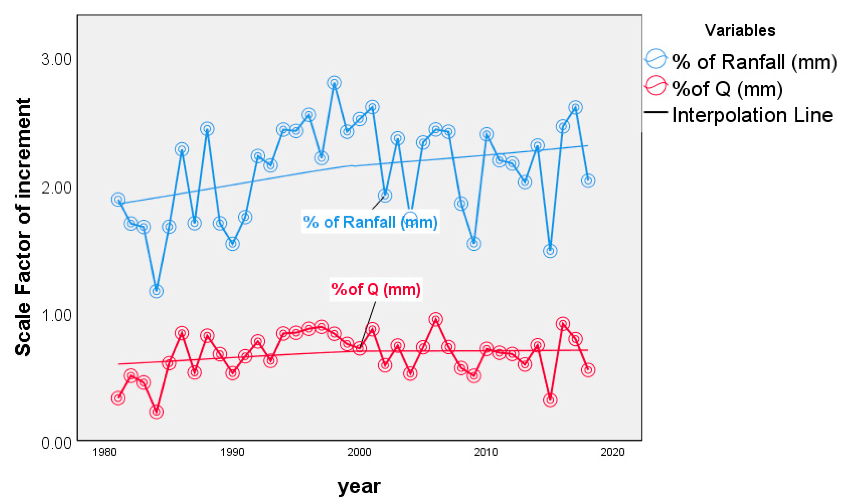
Temporal scale factor increments of percentage rainfall and percentage runoff (Q).


Table 1.
Mean climate data from 1981–2018 years of the study area.
| Month | Average Temperature (°C) | Min. Temperature (°C) | Max. Temperature (°C) | Precipitation (mm) |
|---|---|---|---|---|
| January | 15.5 | 6.8 | 24.2 | 22.98 |
| February | 15.7 | 7.4 | 24.1 | 13.6 |
| March | 17.1 | 8.8 | 25.4 | 60.2 |
| April | 17.8 | 10.3 | 25.4 | 81 |
| May | 19.4 | 10.3 | 28.5 | 61.13 |
| June | 20.6 | 11.5 | 29.7 | 46.6 |
| July | 19.3 | 13.3 | 25.3 | 231.4 |
| August | 18.5 | 12.3 | 24.7 | 280.4 |
| September | 18 | 10.6 | 25.4 | 82.12 |
| October | 16.3 | 7.5 | 25.1 | 47.7 |
| November | 15.9 | 6.4 | 25.4 | 20.6 |
| December | 15.1 | 6.3 | 24 | 44.3 |
Table 2.
Landsat images used for the analysis of land use and land cover (LULC) (Source: http://glovis.usgs.gov).
Table 2.
Landsat images used for the analysis of land use and land cover (LULC) (Source: http://glovis.usgs.gov).
| Sensor | Month/Day/Year | Resolution | Path /Row |
|---|---|---|---|
| Landsat 5 TM | 12/15/1986 | 30 m | 168/51 |
| Landsat 5 TM | 01/28/2001 | 30 m | 168/51 |
| Landsat 8 OLI | 01/13/2018 | 30 m | 168/51 |
Table 3.
Classification of hydrologic soil groups.
| Soil Group | Characteristics |
|---|---|
| A | Low overland flow potential, high minimum infiltration capacity even when thoroughly wetted (> 0.76 cm/h) Deep, well, to excessively drained sands and gravel. |
| B | Moderate minimum infiltration capacity when thoroughly wetted (0.13–0.76 cm/h) Moderately deep to deep Moderately to well drained Moderately fine to moderately coarse grained (e.g., sandy loam). |
| C | Low minimum infiltration capacity when thoroughly wetted (0.13–0.38 cm/h) Moderately fine to fine grained soils or soils with an impeding layer (fragipan). |
| D | High overland flow potential Very low/minimum infiltration capacity when thoroughly wetted (<0.13 cm/h) Clay soils with high swelling potential Soils with permanent high-water table Soils with a clay layer near the surface Shallow soils over impervious bedrock. |
Source: Dingman [84].
Table 4.
Runoff curve numbers for antecedent moisture condition (AMC II) for the study area.
| Land Use Type | Texture | HSG | CN | Area | LU% |
|---|---|---|---|---|---|
| Bare | Clay | D | 89 | 160 | |
| Bare | Clay loam | D | 89 | 370 | |
| Bare | Loam | B | 82 | 2 | |
| Sub Total | 532 | 0.96 | |||
| Built-up | Clay | D | 98 | 71 | |
| Built-up | Clay loam | D | 98 | 257 | |
| Sub Total | 328 | 0.59 | |||
| Cultivation | Clay | D | 91 | 10,117 | |
| Cultivation | Clay loam | D | 91 | 12,262 | |
| Cultivation | Loam | B | 81 | 72 | |
| Cultivation | Sandy clay | A | 72 | 5 | |
| Cultivation | Sandy clay loam | C | 88 | 6 | |
| Sub Total | 22,462 | 40.53 | |||
| Forest | Clay | D | 83 | 2677 | |
| Forest | Clay loam | D | 83 | 9470 | |
| Forest | Sandy clay loam | C | 77 | 6 | |
| Sub Total | 12,153 | 21.93 | |||
| Grass | Clay | D | 80 | 532 | |
| Grass | Clay loam | D | 80 | 1011 | |
| Grass | Sandy clay | A | 39 | 3 | |
| Sub total | 1546 | 2.79 | |||
| Shrub | Clay | D | 89 | 4770 | |
| Shrub | Clay loam | D | 89 | 13,490 | |
| Shrub | Loam | B | 79 | 2 | |
| Shrub | Sandy clay | A | 68 | 13 | |
| Shrub | Sandy clay loam | C | 86 | 4 | |
| Sub Total | 18,279 | 32.98 | |||
| Water | Clay | D | 100 | 37 | |
| Water | Clay loam | D | 100 | 82 | |
| Sub Total | 119 | 0.21 | |||
| Total | 55,419 | 100 |
Table 5.
Land use and land cover (LULC) dynamics of the dry Afromontane forest.
| LULC class | Percentage of Land Cover (%) | Change | ||||
|---|---|---|---|---|---|---|
| 1986 | 2001 | 2018 | 1986–2018 | 1986–2001 | 2001–2018 | |
| Bare | 0.00 | 0.24 | 0.94 | +0.94 | +0.24 | +0.70 |
| Built-up | 0.05 | 0.30 | 0.58 | +0.53 | +0.25 | +0.28 |
| Cultivation | 42.02 | 36.79 | 39.56 | −2.46 | −5.24 | +2.77 |
| Forest | 4.72 | 23.87 | 21.40 | +16.68 | +19.14 | +2.47 |
| Grass | 2.25 | 2.73 | 2.75 | +0.49 | +0.48 | +0.02 |
| Shrub | 48.51 | 33.49 | 32.18 | −16.33 | −15.02 | −1.31 |
| Water | 2.44 | 2.59 | 2.60 | +0.16 | +0.15 | +0.01 |
| Total | 100 | 100 | 100 | |||
Table 6.
Impact of rainfall and potential evapotranspiration on runoff coefficients.
| Variable | Coefficients(B) | Std. Error | T | Sig. |
|---|---|---|---|---|
| Constant | 0.290 | 0.80 | 3.640 | 0.001 |
| Rainfall | 0.837 | 0.061 | 10.754 | 0.000 |
| PET | −0.240 | 0.095 | −2.533 | 0.016 |
| Regression (Sum of Squares) | 814 | 0.00 | ||
| Residual (Sum of Squares) | 133 | 0.00 | ||
| F-test | 63.482 | |||
Table 7.
Pearson’s coefficient of correlation between discharge and climatic parameters.
| Year | Rainfall | Q | PET | Min To | Max To | ||
|---|---|---|---|---|---|---|---|
| Year | Pearson Correlation | 1 | |||||
| Sig. (2-tailed) | |||||||
| Rainfall | Pearson Correlation | .361* | 1 | ||||
| Sig. (2-tailed) | .026 | ||||||
| Q | Pearson Correlation | .263 | .863** | 1 | |||
| Sig. (2-tailed) | .110 | .000 | |||||
| PET | Pearson Correlation | .032 | −.076 | −.264 | 1 | ||
| Sig. (2-tailed) | .848 | .648 | .021 | ||||
| Min T | Pearson Correlation | −.044 | −.271 | −.061 | −.385* | 1 | |
| Sig. (2-tailed) | .795 | .100 | .715 | .017 | |||
| Max T | Pearson Correlation | .032 | −.076 | −.264 | 1.000** | −.385* | 1 |
| Sig. (2-tailed) | .848 | .648 | .109 | .000 | .017 | ||
| N | 38 | 38 | 38 | 38 | 38 | 38 | |
* Correlation is significant at the 0.05 level (2-tailed); ** Correlation is significant at the 0.01 level (2-tailed).
Table 8.
Characteristics of monthly and annual rainfall P and stream discharge flow (Q) in Hugumburda Grat Kahisu state forest Northern, Ethiopia (1981–2018).
Table 8.
Characteristics of monthly and annual rainfall P and stream discharge flow (Q) in Hugumburda Grat Kahisu state forest Northern, Ethiopia (1981–2018).
| January | Februay | March | April | May | June | July | August | September | October | November | December | Annual Average | ||
|---|---|---|---|---|---|---|---|---|---|---|---|---|---|---|
| Discharge flow (Q) | Mean | 0.053 | 0.153 | 0.518 | 0.888 | 0.784 | 0.15 | 2.89 | 2.99 | 0.382 | 0.26 | 0.07 | 0.07 | 0.78 |
| Minimum | 0.00 | 0.00 | 0.00 | 0.00 | 0.00 | 0.00 | 0.00 | 0.00 | 0.00 | 0.00 | 0.00 | 0.00 | 0.00 | |
| Maximum | 6.36 | 13.13 | 32.50 | 45.75 | 40.06 | 27.03 | 56.40 | 37.69 | 18.63 | 27.04 | 13.18 | 15.29 | 56.40 | |
| Std. Error of Mean | 0.008 | 0.03 | 0.075 | 0.11 | 0.09 | 0.05 | 0.19 | 0.12 | 0.04 | 0.05 | 0.018 | 0.0208 | 0.026 | |
| Rainfall | Mean | 0.51 | 0.76 | 1.56 | 2.44 | 2.11 | 0.65 | 6.42 | 7.07 | 1.70 | 1.02 | 0.47 | 0.38 | 2.11 |
| Minimum | 0.00 | 0.00 | 0.00 | 0.00 | 0.00 | 0.00 | 0.00 | 0.00 | 0.00 | 0.00 | 0.00 | 0.00 | 0.00 | |
| Maximum | 18.92 | 30.59 | 53.06 | 68.04 | 61.69 | 48.68 | 81.77 | 60.82 | 37.26 | 48.68 | 30.67 | 31.97 | 81.77 | |
| Std. Error of Mean | 0.054 | 0.09 | 0.17 | 0.23 | 0.200 | 0.098 | 0.37 | 0.29 | 0.1242 | 0.12 | 0.064 | 0.061 | 0.057 | |
© 2019 by the authors. Licensee MDPI, Basel, Switzerland. This article is an open access article distributed under the terms and conditions of the Creative Commons Attribution (CC BY) license (http://creativecommons.org/licenses/by/4.0/).
Share and Cite
MDPI and ACS Style
Gebru, B.M.; Lee, W.-K.; Khamzina, A.; Lee, S.-g.; Negash, E. Hydrological Response of Dry Afromontane Forest to Changes in Land Use and Land Cover in Northern Ethiopia. Remote Sens. 2019, 11, 1905. https://doi.org/10.3390/rs11161905
AMA Style
Gebru BM, Lee W-K, Khamzina A, Lee S-g, Negash E. Hydrological Response of Dry Afromontane Forest to Changes in Land Use and Land Cover in Northern Ethiopia. Remote Sensing. 2019; 11(16):1905. https://doi.org/10.3390/rs11161905
Chicago/Turabian StyleGebru, Belay Manjur, Woo-Kyun Lee, Asia Khamzina, Sle-gee Lee, and Emnet Negash. 2019. "Hydrological Response of Dry Afromontane Forest to Changes in Land Use and Land Cover in Northern Ethiopia" Remote Sensing 11, no. 16: 1905. https://doi.org/10.3390/rs11161905
Note that from the first issue of 2016, this journal uses article numbers instead of page numbers. See further details here.