Optimal Timing Assessment for Crop Separation Using Multispectral Unmanned Aerial Vehicle (UAV) Data and Textural Features


Department of Geography, Remote Sensing Laboratories (RSL), University of Zürich, Winterthurerstrasse 190, 8057 Zürich, Switzerland
*
Author to whom correspondence should be addressed.
Remote Sens. 2019, 11(15), 1780; https://doi.org/10.3390/rs11151780
Submission received: 17 May 2019
/
Revised: 25 July 2019
/
Accepted: 27 July 2019
/
Published: 30 July 2019
(This article belongs to the Special Issue Remote Sensing for Crop Mapping)
Abstract
:The separation of crop types is essential for many agricultural applications, particularly when within-season information is required. Generally, remote sensing may provide timely information with varying accuracy over the growing season, but in small structured agricultural areas, a very high spatial resolution may be needed that exceeds current satellite capabilities. This paper presents an experiment using spectral and textural features of NIR-red-green-blue (NIR-RGB) bands data sets acquired with an unmanned aerial vehicle (UAV). The study area is located in the Swiss Plateau, which has highly fragmented and small structured agricultural fields. The observations took place between May 5 and September 29, 2015 over 11 days. The analyses are based on a random forest (RF) approach, predicting crop separation metrics of all analyzed crops. Three temporal windows of observations based on accumulated growing degree days (AGDD) were identified: an early temporal window (515–1232 AGDD, 5 May–17 June 2015) with an average accuracy (AA) of 70–75%; a mid-season window (1362–2016 AGDD, 25 June–22 July 2015) with an AA of around 80%; and a late window (2626–3238 AGDD, 21 August–29 September 2015) with an AA of <65%. Therefore, crop separation is most promising in the mid-season window, and an additional NIR band increases the accuracy significantly. However, discrimination of winter crops is most effective in the early window, adding further observational requirements to the first window.
1. Introduction
Crop type separation is a crucial requirement for the planning [1], short-term monitoring [2], management [3], high-throughput phenotyping [4,5,6], and climate change modeling [7] of agricultural areas. Many of these tasks need up-to-date information, in particular before the end of the growing season. These tasks require spatially explicit land cover maps. Nevertheless, this kind of information is usually reported by farmers only after the season and mostly at administrative units [8]. Even when the reporting for subsidies takes place in a geographic information system, as is the case in Switzerland, the data are only entered after the season or even in the following year [9]. Therefore, a more up-to-date assessment of crop status needs a different data collection source.
Remote sensing has proven its potential to deliver such information even before the end of season [10]. Land cover crop maps are often based on satellite data because these platforms provide data sets multiple times per month and are suitable for both single-date or multitemporal classification tasks [11,12]. Moreover, several studies have demonstrated the ability to carry out early stage crop mapping [1,2,13,14]. However, due to fixed orbits and thus fixed observation dates, clouds can limit the amount of usable data. Furthermore, freely available data from Landsat or Sentinel satellites have coarse spatial resolution and therefore capture a high amount of mixed pixel information, especially in small structured farmlands. Hence, data sets of higher spatial resolution are necessary to acquire spectrally pure pixels that are needed in algorithm training [10,15,16]. To date, data sets gained with spaceborne sensors at an appropriate spatial resolution are still expensive and rare.
Unmanned aerial vehicles (UAVs) deliver spatially very high resolution (VHR) data sets and a 3D point-cloud with a spatial resolution of only a few centimeters [17]. UAV data creates new opportunities in agriculture [18,19,20], e.g., assessment of plant health status [21], water stress [22], management techniques [23], erosion of soils [24], and detection of individual plants [25], among many others. The advantages of VHR data sets compared to common satellite data sets have also been analyzed, e.g., for vegetation indices (VI) [26,27]. Further, UAVs have the ability to acquire data in a very flexible manner, e.g., by considering changing weather conditions, and they are cheap to operate compared to other carrier systems [17]. However, less sophisticated sensors are usually mounted on UAVs, containing broader spectral bands that are difficult to spectrally and radiometrically calibrate [28]. Consumer-grade cameras provide red, green and blue (RGB) wavelength bands, but they can be modified in a way to be able to acquire a near-infrared (NIR) band as well [29]. Therefore, a NIR-RGB mosaic can be built using combined data from these two camera types.
In Switzerland, farmland is often structured in small plots [30], and therefore VHR data sets are required to accurately discriminate different crops. To acquire VHR data sets for multiple dates, consumer-grade cameras with RGB and NIR-GB bands were mounted on a UAV. Uncalibrated data sets were used in this study to investigate the potential of a straightforward, user-friendly, and low-cost data acquisition and processing methodology for crop separation over a growing season. Due to the sensors’ limited spectral properties, the incorporation of additional information content through textural features is a promising option to improve the accuracy of crop separation [31,32].
Using approaches, in which all available remotely sensed data sets are jointly processed for crop classification purposes, the accuracy of crop separation has been found to increase [1,11,12,14]. In very fragmented agricultural systems, with very small fields, inhomogeneous cropping cycles and stringent crop rotation schemes, such as on the Swiss Plateau, sawing and harvesting dates of crops are subject to large temporal variations and arbitrarily changing patterns of bare vs. vegetated land cover. These properties are resulting in a decrease of the overall accuracy of crop separation by more than 20% (data not shown) on the Swiss Plateau when using a stacked approach.
Since crops show a changing spectral response due to the evolution of their phenological stage over the growing season, we hypothesize that crops can be separated with varying accuracy at different observation dates over the season. Hence, the aims of this study are to (i) determine an optimal temporal window during the growing season to separate all present crop types from each other, including textural features of an uncalibrated NIR-RGB data set, (ii) evaluate the potential of an additional NIR band compared to a standard RGB configuration, and (iii) assess the potential to discriminate a single crop type from all others on different observation dates.
2. Materials and Methods
2.1. Study Area
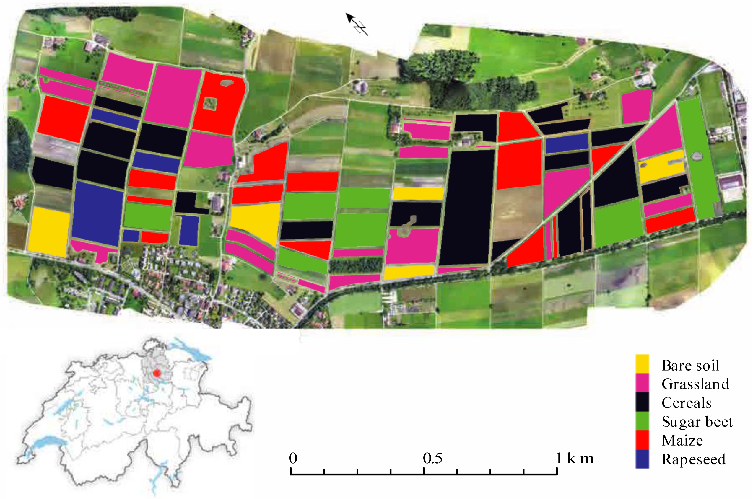
The study area is located on the Swiss Plateau (47.312°N, 8.733°E, Figure 1) and is subject to a warm temperate humid climate [33]. Crop and grasslands mainly dominate the area. The crop types include winter and summer crops. Winter crops are cereals (winter barley, spelt, and winter wheat), rapeseed, and grassland (permanent and temporary, including clover), whereas the summer crops taken into account in this study are maize and sugar beet. For maize, rapeseed, sugar beet, and winter wheat (which represents the cereal crop type), the phenological stage of a single reference field was recorded according to the Biologische Bundesanstalt, Bundessortenamt und Chemische Industrie (BBCH) scale for all 11 observation dates between 5 May 5 and 29 September 2015 (Table 1) [34].
The total number of fields for a specific crop varied between observation dates; some grassland fields were transformed first into bare soil fields before being sown as summer crop fields (i.e., sugar beet or maize). Other fields were harvested on a certain date and changed therefore to bare soil, or were sown with grass again. Fields with crop residuals were still treated as the previously harvested crop (e.g., cereals after harvesting and before they were cleared as bare soil in preparation for the planting of a next crop). Consequently, there were no bare soil fields present on May 5, July 3, and July 10. Nevertheless, the total number of fields remained the same over the entire study period.
The agricultural area is structured into small fields ranging from 0.03 to 7.4 ha with an average size of 1.3 ha. The length of a single field varies between 140 m and 200 m and the width between 23 m and 180 m. The total area and number of fields for each class is given in Table 2 for 25 June 2015.
2.2. Data
The image data sets were acquired with an eBee-UAV (Sensefly, Cheseaux-Lausanne, Switzerland) under sunny conditions and two consumer-grade cameras (Canon IXUS 125HS) that record NIR-GB and RGB bands. Image acquisition was performed with the software eMotion2 (Sensefly, Cheseaux-Lausanne, Switzerland), in which the flight altitude was set to 150 m above ground with a lateral overlap of 60% and a longitudinal overlap of 75%, resulting in a spatial resolution of 5 cm (nominal cruise speed 11–25 m/s). Subsequently, an ortho-photomosaic was generated for each observation date with Pix4Dmapper Pro (version 4.2.27, Pix4D S.A., Prilly, Switzerland), combining the NIR band of the one camera and the RGB bands of the other. The data set collected on June 25 was georeferenced on the basis of five ground control points (GCP) measured with a differential GPS device (dGPS), and the other data sets were subsequently georeferenced to this data set. Finally, these data sets were resampled to a spatial resolution of 0.5 m, a spatial resolution most suitable for discrimination of the present crops [32].
2.3. Methodology
In order to decouple the observation date from the phenological stage of the different investigated crops, a growing degree days (GDD) metric was used. GDD was calculated based on temperature data of the closest weather station (Zurich Fluntern, <20 km, Source: Swiss Federal Office of Meteorology and Climatology) with a base temperature TB of 5.5 °C, the minimal growing temperature for the majority of the crops in the study area [35].
GDD was calculated for an individual day (d) based on the method of [35]
with TMd being the mean temperature at day d. For each observation date the accumulated GDD (AGDD) was calculated as
with n being the number of days between March 1 and the particular observation date (Table 1).
To incorporate contextual information, two types of features were generated for all spectral bands, i.e., first-order statistics (mean, standard deviation, range, and entropy), and mathematical morphology (dilatation/erosion, opening/closing, opening/closing top hat, opening/closing by reconstruction, and opening/closing by reconstruction top hat). To extract rotation invariant features, a disc-shaped structuring element (SE) was applied with diameters of 3 and 5 pixels [36].
For each observation date, two band settings were built, one with all four bands (NIR-RGB) and one with the RGB bands only, each with the spatial features of the two SE sizes. The data set was subdivided class-wise into six splits and all 15 possible permutations for the selection of two splits for testing were built. Of the remaining four splits per class, two were used for training and two for validation in the classification model building. For the subsequent crop separation, a random forest (RF) algorithm was used [37] since it has been successfully applied in previous studies [38].
In order to determine the best parameters for the RF model, i.e., the number of trees, the results of models with 20 grid points for the number of trees distributed logarithmically between 10 and 1000 were evaluated. Finally, the number of trees was chosen in a way that the loss of accuracy was less than 0.1% compared to the maximum accuracy of the curve fitted to the grid points [32]. The minimal leaf size in the TreeBagger function was set to three, and for the other parameters the default settings from the MATLAB implementation were chosen [39]. The final model was applied to the test data split. A detailed description of the method can be found in [32].
The assessments of the accuracy metrics are based on the average accuracy (AA) and the user accuracy (UA) in order to focus on the needs of potential users. The values are retrieved from the confusion matrix of the classification results of the test data splits and averaged over all 15 folds. In addition, the results for overall accuracy (OA), Kappa coefficient, producer accuracy (PA), and average reliability (AR) are presented in the Appendix A (Table A1).
The entire workflow from feature calculation to crop separation and accuracy assessment for the data set of a single observation date was applied to all 11 data sets. In order to evaluate the differences in crop discrimination accuracy between the different observation dates and settings, the accuracy measurements of the single data sets were tested for significance (p < 0.05) against each other using the Wilcoxon signed rank test. A temporal window during the growing season to separate all crop types from each other was defined on subjective visual impression of the AA at the available observation dates (cf. Figure 2).
3. Results
The accuracy results (i.e., AA and UA) can be found in Table 3 for the two band settings (i.e., NIR-RGB and RGB, including spatial features of the two SE sizes). The OA, Kappa, and AR metrics are reported in Table A1 in the Appendix A, as well as the p-values of the significance tests (Wilcoxon signed rank test) between the observation dates for each of the two band settings (Table A2 and Table A3), and between the NIR-RGB and RGB settings (Table A4).
3.1. Temporal Windows during the Growing Season
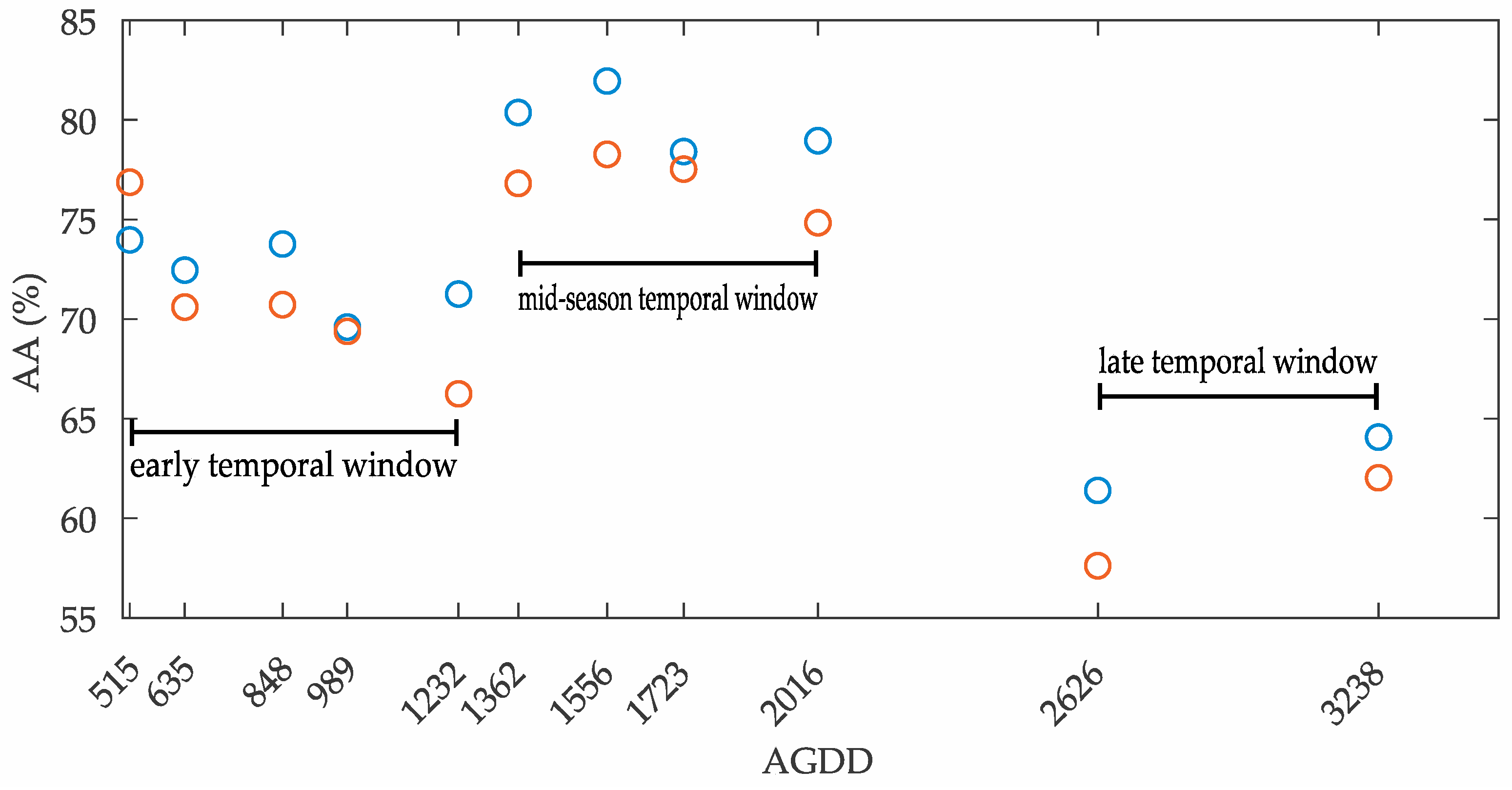
Based on the AA metric, three temporal windows during the growing season were identified, i.e., an early temporal window from 515 to 1232 AGDD, a mid-season temporal window from 1362 to 2016 AGDD, and a late temporal window from 2626 to 3238 AGDD (Figure 2). The mid-season window shows the highest crop separation potential with an average AA value of 79.9% over the four observation dates for the NIR-RGB setting and an average AA value of 76.9% for the RGB setting. At 1556 AGDD, the maximum AA values of 82.0% and 78.3% are reached for the NIR-RGB setting and for the RGB setting, respectively (Table 3).
The five observations in the early temporal window until 1232 AGDD contain slightly lower AA values. The average AA values in this time frame are 7.7% lower for the NIR-RGB setting compared to the mid-season temporal window and, correspondingly, 14.2% lower for the RGB setting. The lowest AA values are found in the late temporal window at 62.7% and 59.8% for the NIR-RGB and RGB settings, respectively.
For the NIR-RGB setting, the AA values within a given temporal window are fairly stable but vary significantly between the three temporal windows (Table A2). In contrast, the AA values for the RGB setting are significantly less stable within both the early and late temporal windows. The AA value for the observation at 515 AGDD is not significantly different from the AA values of the mid-season, and the AA value for 1232 AGDD is not significantly different from the AA value at 3238 AGDD (Table A3).
In the early temporal window, the accuracy of the crop discrimination slightly decreases over time by 4.4% for the NIR-RGB setting (Table 3). The highest performance is achieved at 515 AGDD with an AA of 74.0%. The lowest performance is achieved at 989 AGDD with an AA of 69.6%. In case of the RGB setting, the AA values decrease by over 10% between the highest AA of 76.9% at 515 AGDD and the lowest AA of 66.3% at 1232 AGDD.
Regarding the NIR-RGB setting within the early temporal window, only the AA value at 848 AGDD is significantly different from the one at 1232 AGDD (Table A2). For the RGB setting, the AA value for the observation at 515 AGDD is significantly higher than all other AA values in the early temporal window, whereas the AA value of the observation at 1232 AGDD is significantly lower than the AA values at 515, 635, and 848 AGDD (Table A3).
In the mid-season temporal window, the highest AA values are achieved at 1556 AGDD with 82.0% in case of the NIR-RGB setting and 78.3% in case of the RGB setting (Table 3). The lowest AA values are at 1723 AGDD with 78.4% in case of the NIR-RGB setting and at 2016 AGDD with 74.8% in case of the RGB setting. There are no significant differences between the AA values, except for the highest AA at 1556 AGDD that is significantly higher than the AA values at 1723 and 2016 AGDD for the NIR-RGB setting (Table A2). For the RGB setting, the AA value at 2016 AGDD is significantly lower than the AA values at 1556 and 1723 AGDD (Table A3). All other AA values in this temporal window are not significantly different from each other.
In the late temporal window, the AA values for both band settings are lower than the AA values in the other temporal windows (Table 3), and there is no significant difference between the AA value at 2626 and 3238 AGDD in the case of the NIR-RGB setting (Table A2). As for the RGB setting, the AA value at 3238 AGDD is significantly higher (by as much as 4.4%) than the AA value at 2626 AGDD (Table A3).
3.2. Band Settings
Considering the two investigated band settings, only minor differences in the temporal evolution of the respective AA values are found over the growing season. In the early temporal window, a minimum AA value of 69.9% is reached at 989 AGDD for the NIR-RGB setting, and a minimum AA value of 66.3% at 1232 AGDD in case of the RGB setting. For both settings, the AA values increase significantly between 1232 and 1362 AGDD when they reach the mid-season temporal window. They then fall to low values of 2626 AGDD. Overall, the additional NIR band leads to significantly better results for crop separation in terms of AA values for all observation dates at a significance level of p < 0.05, except for the observations at 515 and 989 AGDD (Table A4).
3.3. Discrimination of Individual Crop Types
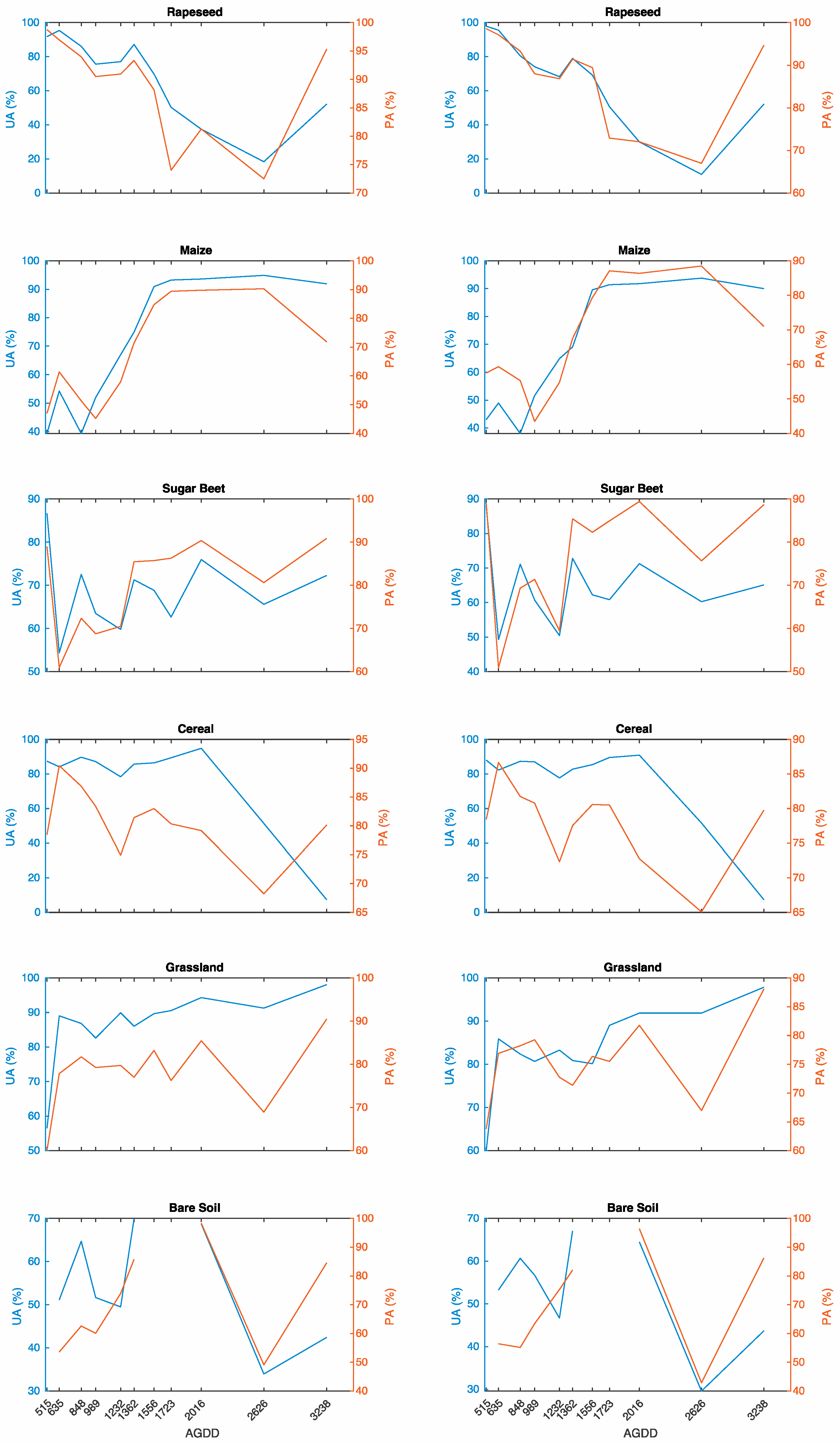
The temporal assessment of the ability to separate a single crop from the others is very similar for both band settings (Figure 3). Rapeseed can be distinguished best in early season with a UA of over 90% until 635 AGDD. Afterwards, the UA remains above 70% until 1556 AGDD, when it decreases to a minimum of less than 20% at 2626 AGDD. On the contrary, maize can easily be discriminated after 1556 AGDD, with the UA increasing from under 75% to over 90%.
The discrimination of sugar beet is most effective at 515 AGDD with a UA of more than 85%. At 635 AGDD, its discrimination is most difficult with a UA of less than 55%. From 848 AGDD onwards, the UA lies between 60% and 76% except for in the case of the RGB setting, when the UA is 50.5% at 1232 AGDD.
Cereals can be distinguished with a UA between 78% and 90% from the beginning of the analyzed AGDD until 1723 AGDD. At 2016 AGDD, the UA is highest with 94.9% for the NIR-RGB setting and 91% for the RGB setting. At 2626 AGDD, the UA is around 51%, and for the last observation date it drops to 7%.
The UA of grassland is under 60% at 515 AGDD, but increases to a range of 80% to 94% from 635 AGDD onwards. On the final observation date, the UA is highest at 98%.
Bare soil can best be discriminated at 1362 and 2016 AGDD with UA values between 65% and 70%. Earlier, the UA is around 55%; it is only higher at 848 AGDD, reaching 65% for the NIR-RGB setting and 61% for the RGB setting. The UA is under 50% for the last two observation dates.
4. Discussion
4.1. Temporal Windows During the Growing Season
The phenological stage of crops is essential to discriminate them from each other in remote sensing data analysis. When considering all of the crops in the study area, the accuracy of crop separation is highest in the mid-season temporal window between 1362 and 2016 AGDD but accuracy reaches a maximum at 1556 AGDD. This is in line with other studies that report best accuracies for crop separation with data sets acquired in July [2,40,41]. At this time of the growing season, the winter crops are in a senescence stage and the summer crops in their most productive stage.
In the early temporal window, at the beginning of the growing season, maize and sugar beet are gradually sown in. Since their seedlings are difficult to distinguish [40] and can thus be mixed up with pixels from bare soil fields, the AA values are lower than in the subsequent mid-season temporal window. The slight decrease in AA values in the early temporal window is not of statistical significance.
Apart from a few exceptions, crop separation accuracies within a temporal window are not significantly different from the other observations in the same temporal window. This holds true for the two tested band settings and their textural features of the UAV data sets. Consequently, any observation of crops within a given temporal window will yield a similar, not significantly different AA.
4.2. Band Settings
An additional NIR band leads to significantly higher crop separation accuracies for most of the observation dates, as reported in several other studies [42,43,44]. Only at 515 AGDD does the AA value of the RGB setting become higher than in the case of the NIR-RGB setting. Since this difference is not significant, crop separation accuracy with an additional NIR band is generally higher, or at least equal to an RGB setting.
In land use/land cover classifications that are based on textural features, the applied SE sizes play a crucial role [32]. Differing spectral signatures resulting from the interplay of plant material and soil background largely define textural information in agricultural fields. Consequently, when the crop canopy is closed, the spectral, rather than the textural, properties gain in importance [45] and therefore, an additional NIR band can lead to an improvement in crop separation [43].
4.3. Discrimination of Individual Crop Types
With regard to the separation of individual crop species, their own respective phenological stages are crucial. Rapeseed, for example, produces yellow flowers up to 635 AGDD and can therefore be distinguished from all other crops with high precision, as it is the only investigated crop with this specific color. The discrimination of cereals in general, being the other winter crops in the study area, is best straight after harvesting at 2016 AGDD when the signal is dominated by the crop residuals and bare soil, and summer crops (i.e., sugar beet and maize) are in their most productive stage.
The differences between individual summer crops get more pronounced with phenological development; therefore, the UA values of maize and sugar beet increase with generally increasing AGDDs. As reported by [46], the UA of maize increases by over 50% between the first discrimination, when maize fields are freshly sown in at 515 AGDD, and before harvesting at 2626 AGDD, when all other fields are either bare soil or covered by green grassland or sugar beet.
Sugar beet is the first sown summer crop in the study area and can be accurately separated at 515 AGDD, as the spectral signal is dominated by bare soil and therefore is distinguishable from the other present crops (i.e., winter crops or grassland). At the following observation date (i.e., 635 AGDD), differentiation between maize, sugar beet and bare soil fields becomes more difficult, since the spectral signal of all three classes at this phenological stage is dominated by the signal of bare soil and indistinguishable seedlings [40].
Overall, the UA value of grassland is highest after 3238 AGDD, since late in the season it is the only crop well distinguishable from bare soil, maize (appearing brown in its final phenological stages), and sugar beet. In addition, grassland covers most of the area in late season so, consequently, the OA is also high (Table A1). Nevertheless, the AA metric, which gives equal weight to the UA values of all present crop types, is low because the other crops can no longer be distinguished accurately from each other.
Finally, bare soil can most accurately be separated from crops when their plant materials cover a large part of the area and therefore dominate the measured signal. It is particularly difficult to distinguish fields under preparation (e.g., plowed) from fields containing small seedlings. The discrimination of cereals shortly after harvesting is successful since the textural appearance of crop residuals and bare soil is different. Therefore, discrimination of bare soil is most successful at 1362 and 2016 AGGD.
4.4. Limitations and Outlook
Crop types present in an agricultural area influence the resulting separation accuracy. The more diverse they are in terms of morphology and physiology, the more accurately they can be discriminated. Consequently, it is more challenging to separate between different winter crops or between different summer crops than to differentiate winter crops from summer crops. In particular, further separation of crops that have been combined into one class in this study (e.g., cereals like winter wheat, spelt and winter barley) remains to be investigated. Moreover, the optimal temporal windows analyzed here may vary depending on the specific crop types present in an agricultural area, and the behavior between the windows must be further examined.
As shown in a range of other studies, multitemporal data sets improve the accuracies of crop classification tasks [41,47]. Therefore, it would be interesting to investigate the potential of combining data from different acquisition dates to find the most promising temporal combinations for crop separation. Due to the fact that observations with optical sensors are subject to limitations (e.g., cloudy conditions), combined analysis of data acquired in the early and mid-season temporal windows could be promising.
5. Conclusions
This paper presents a methodology to separate agricultural crops based on data sets acquired with uncalibrated consumer-grade cameras mounted on a UAV over the course of 11 observation dates between 5 May 2015 (515 AGDD) and 29 September 2015 (3238 AGDD). The obtained four bands data sets, consisting of a NIR, red, green, and blue band, were extended with textural features to differentiate cereals, grassland, maize, rapeseed and sugar beet, and, if present, bare soil, based on an RF approach.
Three temporal windows across the growing season were identified where the accuracies of crop separation between the observation dates were not significantly different. The first temporal window ranged from 515 AGDD (May 5) to 1232 AGDD (June 17), with an AA for separation between 70% and 75%. A mid-season temporal window between 1362 AGDD (June 25) and 2016 AGDD (July 22) proved to be the most optimal for crop separation with AA values around 80%. Observations after 2626 AGDD (August 21) fell into the third group with an AA of under 65%.
An additional NIR band leads to significantly higher separation results compared to a pure RGB setting, thanks to an extended capability to spectrally discriminate the plant materials of the various crops. The accuracy of the separation of single crops varies over the course of the observed period. Winter crops can be discriminated from summer crops more accurately in the early season, whereas the accuracy of single summer crop separation from other summer crops is highest during their most productive phenological stage in the mid-season temporal window.
Overall, this paper concludes that crop separation based on uncalibrated NIR-RGB data sets in a highly fragmented and small structured agricultural area like the Swiss Plateau is most accurate between 1362 AGDD and 2016 AGDD over the investigated period.
Author Contributions
J.E.B. designed the research and analyzed the data with scientific advice of M.K. and M.E.S., J.E.B. wrote the manuscript and all co-authors thoroughly reviewed and edited the manuscript.
Funding
This research received no external funding.
Acknowledgments
The contribution of M.E.S. is supported by the University of Zurich Research Priority Program on ‘Global Change and Biodiversity’ (URPP GCB). The meteorological data were provided by MeteoSwiss, the Federal Office for Meteorology and Climatology. We thank staff from RSL and GRS (Wageningen University) supporting fieldwork and providing background information. Reinhard Furrer from the Department of Mathematics at UZH is thanked for guidance with statistical analyses.
Conflicts of Interest
The authors declare no conflict of interest.
Appendix A

Table A1.
Overall accuracy (OA), Kappa coefficient, average accuracy (AA), and average reliability (AR) for both settings and all observation dates.
Table A1.
Overall accuracy (OA), Kappa coefficient, average accuracy (AA), and average reliability (AR) for both settings and all observation dates.
| Setting | Observation Date (AGDD) | OA | Kappa | AA | AR |
|---|---|---|---|---|---|
| NIR-RGB | 515 | 77.3 | 0.691 | 74.0 | 74.6 |
| NIR-RGB | 635 | 78.1 | 0.708 | 72.5 | 73.5 |
| NIR-RGB | 848 | 77.9 | 0.719 | 73.8 | 74.8 |
| NIR-RGB | 989 | 73.0 | 0.662 | 69.6 | 71.1 |
| NIR-RGB | 1232 | 73.0 | 0.663 | 71.3 | 74.7 |
| NIR-RGB | 1362 | 80.2 | 0.752 | 80.4 | 82.4 |
| NIR-RGB | 1556 | 84.2 | 0.795 | 82.0 | 84.9 |
| NIR-RGB | 1723 | 82.2 | 0.770 | 78.4 | 81.2 |
| NIR-RGB | 2016 | 85.8 | 0.819 | 79.0 | 87.3 |
| NIR-RGB | 2626 | 75.1 | 0.671 | 61.4 | 71.6 |
| NIR-RGB | 3238 | 85.8 | 0.766 | 64.1 | 85.5 |
| RGB | 515 | 78.8 | 0.713 | 76.9 | 77.5 |
| RGB | 635 | 75.7 | 0.676 | 70.6 | 71.2 |
| RGB | 848 | 74.3 | 0.674 | 70.7 | 72.1 |
| RGB | 989 | 72.5 | 0.656 | 69.4 | 71.0 |
| RGB | 1232 | 68.4 | 0.607 | 66.3 | 70.3 |
| RGB | 1362 | 76.5 | 0.707 | 76.8 | 79.2 |
| RGB | 1556 | 80.0 | 0.741 | 78.3 | 81.6 |
| RGB | 1723 | 81.1 | 0.756 | 77.5 | 80.1 |
| RGB | 2016 | 81.7 | 0.767 | 74.8 | 83.1 |
| RGB | 2626 | 72.4 | 0.637 | 57.6 | 67.7 |
| RGB | 3238 | 83.9 | 0.738 | 62.0 | 84.8 |
Table A2.
p-values of significance test (p < 0.05) for all observation dates of the NIR-RGB setting. Not significant differences are marked in bold. The green color depicts the three temporal windows (i.e., early, medium and late) over the growing season.
Table A2.
p-values of significance test (p < 0.05) for all observation dates of the NIR-RGB setting. Not significant differences are marked in bold. The green color depicts the three temporal windows (i.e., early, medium and late) over the growing season.
| AGDD | 515 | 635 | 848 | 989 | 1232 | 1362 | 1556 | 1723 | 2016 | 2626 | 3238 |
|---|---|---|---|---|---|---|---|---|---|---|---|
| 515 | 0.107 | 0.934 | 0.169 | 0.107 | 0.005 | 0.001 | 0.018 | 0.030 | 0.000 | 0.002 | |
| 635 | 0.107 | 0.489 | 0.421 | 0.421 | 0.000 | 0.000 | 0.001 | 0.002 | 0.000 | 0.002 | |
| 848 | 0.934 | 0.489 | 0.073 | 0.041 | 0.000 | 0.000 | 0.005 | 0.000 | 0.000 | 0.000 | |
| 989 | 0.169 | 0.421 | 0.073 | 0.489 | 0.000 | 0.000 | 0.001 | 0.000 | 0.000 | 0.035 | |
| 1232 | 0.107 | 0.421 | 0.041 | 0.489 | 0.000 | 0.000 | 0.000 | 0.000 | 0.000 | 0.001 | |
| 1362 | 0.005 | 0.000 | 0.000 | 0.000 | 0.000 | 0.095 | 0.121 | 0.151 | 0.000 | 0.000 | |
| 1556 | 0.001 | 0.000 | 0.000 | 0.000 | 0.000 | 0.095 | 0.001 | 0.002 | 0.000 | 0.000 | |
| 1723 | 0.018 | 0.001 | 0.005 | 0.001 | 0.000 | 0.121 | 0.001 | 0.639 | 0.000 | 0.000 | |
| 2016 | 0.030 | 0.002 | 0.000 | 0.000 | 0.000 | 0.151 | 0.002 | 0.639 | 0.000 | 0.000 | |
| 2626 | 0.000 | 0.000 | 0.000 | 0.000 | 0.000 | 0.000 | 0.000 | 0.000 | 0.000 | 0.151 | |
| 3238 | 0.002 | 0.002 | 0.000 | 0.035 | 0.001 | 0.000 | 0.000 | 0.000 | 0.000 | 0.151 |
Table A3.
p-values of significance test (p < 0.05) for all observation dates of the RGB setting. Not significant differences are marked in bold. The green color depicts the three temporal windows (i.e., early, medium and late) over the growing season.
Table A3.
p-values of significance test (p < 0.05) for all observation dates of the RGB setting. Not significant differences are marked in bold. The green color depicts the three temporal windows (i.e., early, medium and late) over the growing season.
| AGDD | 515 | 635 | 848 | 989 | 1232 | 1362 | 1556 | 1723 | 2016 | 2626 | 3238 |
|---|---|---|---|---|---|---|---|---|---|---|---|
| 515 | 0.003 | 0.003 | 0.001 | 0.001 | 0.934 | 0.359 | 0.762 | 0.330 | 0.000 | 0.000 | |
| 635 | 0.003 | 0.934 | 0.847 | 0.048 | 0.004 | 0.000 | 0.000 | 0.035 | 0.000 | 0.002 | |
| 848 | 0.003 | 0.934 | 0.359 | 0.004 | 0.001 | 0.000 | 0.000 | 0.002 | 0.000 | 0.000 | |
| 989 | 0.001 | 0.847 | 0.359 | 0.151 | 0.003 | 0.000 | 0.000 | 0.008 | 0.000 | 0.001 | |
| 1232 | 0.001 | 0.048 | 0.004 | 0.151 | 0.000 | 0.000 | 0.000 | 0.000 | 0.000 | 0.083 | |
| 1362 | 0.934 | 0.004 | 0.001 | 0.003 | 0.000 | 0.389 | 1.000 | 0.229 | 0.000 | 0.000 | |
| 1556 | 0.359 | 0.000 | 0.000 | 0.000 | 0.000 | 0.389 | 0.454 | 0.000 | 0.000 | 0.000 | |
| 1723 | 0.762 | 0.000 | 0.000 | 0.000 | 0.000 | 1.000 | 0.454 | 0.035 | 0.000 | 0.000 | |
| 2016 | 0.330 | 0.035 | 0.002 | 0.008 | 0.000 | 0.229 | 0.000 | 0.035 | 0.000 | 0.000 | |
| 2626 | 0.000 | 0.000 | 0.000 | 0.000 | 0.000 | 0.000 | 0.000 | 0.000 | 0.000 | 0.008 | |
| 3238 | 0.000 | 0.002 | 0.000 | 0.001 | 0.083 | 0.000 | 0.000 | 0.000 | 0.000 | 0.008 |
Table A4.
p-values of the significance test (p < 0.05) for the difference between the NIR-RGB and RGB setting for overall accuracy (OA), Kappa, average accuracy (AA), and average reliability (AR). Not significant differences are marked in bold.
Table A4.
p-values of the significance test (p < 0.05) for the difference between the NIR-RGB and RGB setting for overall accuracy (OA), Kappa, average accuracy (AA), and average reliability (AR). Not significant differences are marked in bold.
| AGDD | OA | kappa | AA | AR |
|---|---|---|---|---|
| 515 | 0.229 | 0.208 | 0.135 | 0.083 |
| 635 | 0.012 | 0.012 | 0.010 | 0.008 |
| 848 | 0.001 | 0.001 | 0.001 | 0.003 |
| 989 | 0.599 | 0.599 | 0.599 | 0.599 |
| 1232 | 0.000 | 0.000 | 0.000 | 0.000 |
| 1362 | 0.001 | 0.001 | 0.001 | 0.001 |
| 1556 | 0.000 | 0.000 | 0.000 | 0.000 |
| 1723 | 0.001 | 0.001 | 0.003 | 0.000 |
| 2016 | 0.000 | 0.000 | 0.000 | 0.000 |
| 2626 | 0.035 | 0.064 | 0.005 | 0.007 |
| 3238 | 0.000 | 0.000 | 0.000 | 0.012 |
References
- Azar, R.; Villa, P.; Stroppiana, D.; Crema, A.; Boschetti, M.; Brivio, P.A. Assessing in-season crop classification performance using satellite data: A test case in Northern Italy. Eur. J. Remote Sens. 2016, 49, 361–380. [Google Scholar] [CrossRef]
- Ozdarici-Ok, A.; Ok, A.; Schindler, K. Mapping of Agricultural Crops from Single High-Resolution Multispectral Images--Data-Driven Smoothing vs. Parcel-Based Smoothing. Remote Sens. 2015, 7, 5611–5638. [Google Scholar] [CrossRef]
- Inglada, J.; Arias, M.; Tardy, B.; Morin, D.; Valero, S.; Hagolle, O.; Dedieu, G.; Sepulcre, G.; Bontemps, S.; Defourny, P. Benchmarking of algorithms for crop type land-cover maps using Sentinel-2 image time series. 2015 IEEE Int. Geosci. Remote Sens. Symp. 2015, 3993–3996. [Google Scholar] [CrossRef]
- Holman, F.H.; Riche, A.B.; Michalski, A.; Castle, M.; Wooster, M.J.; Hawkesford, M.J. High Throughput Field Phenotyping of Wheat Plant Height and Growth Rate in Field Plot Trials Using UAV Based Remote Sensing. Remote Sens. 2016, 8. [Google Scholar] [CrossRef]
- Shi, Y.; Thomasson, J.A.; Murray, S.C.; Pugh, N.A.; Rooney, W.L.; Shafian, S.; Rajan, N.; Rouze, G.; Morgan, C.L.S.; Neely, H.L.; et al. Unmanned Aerial Vehicles for High-Throughput Phenotyping and Agronomic Research. PLoS ONE 2016, 11, e0159781. [Google Scholar] [CrossRef]
- Tattaris, M.; Reynolds, M.P.; Chapman, S.C. A Direct Comparison of Remote Sensing Approaches for High-Throughput Phenotyping in Plant Breeding. Front. Plant Sci. 2016, 7, 1131. [Google Scholar] [CrossRef]
- Fuhrer, J.; Tendall, D.; Klein, T.; Lehmann, N.; Holzkämper, A. Water Demand in Swiss Agriculture Sustainable Adaptive Options for Land and Water Management to Mitigate Impacts of Climate Change. Art-Schriftenreihe 2013, 19, 56. [Google Scholar]
- Waldhoff, G.; Lussem, U.; Bareth, G. Multi-Data Approach for remote sensing-based regional crop rotation mapping: A case study for the Rur catchment, Germany. Int. J. Appl. Earth Obs. Geoinf. 2017, 61, 55–69. [Google Scholar] [CrossRef]
- Bundesrat, D.S. Verordnung über die Direktzahlungen an die Landwirtschaft. 2017, Volume 2013, pp. 1–152. Available online: https://www.admin.ch/opc/de/classified-compilation/20130216/index.html (accessed on 14 August 2018).
- Atzberger, C. Advances in Remote Sensing of Agriculture: Context Description, Existing Operational Monitoring Systems and Major Information Needs. Remote Sens. 2013, 5, 949–981. [Google Scholar] [CrossRef] [Green Version]
- Zhong, L.; Hu, L.; Zhou, H. Deep learning based multi-temporal crop classification. Remote Sens. Environ. 2019, 221, 430–443. [Google Scholar] [CrossRef]
- Ouzemou, J.E.; El Harti, A.; Lhissou, R.; El Moujahid, A.; Bouch, N.; El Ouazzani, R.; Bachaoui, E.M.; El Ghmari, A. Crop type mapping from pansharpened Landsat 8 NDVI data: A case of a highly fragmented and intensive agricultural system. Remote Sens. Appl. Soc. Environ. 2018, 11, 94–103. [Google Scholar] [CrossRef]
- Löw, F.; Duveiller, G. Defining the spatial resolution requirements for crop identification using optical remote sensing. Remote Sens. 2014, 6, 9034–9063. [Google Scholar] [CrossRef]
- Conrad, C.; Dech, S.; Dubovyk, O.; Fritsch, S.; Klein, D.; Löw, F.; Schorcht, G.; Zeidler, J. Derivation of temporal windows for accurate crop discrimination in heterogeneous croplands of Uzbekistan using multitemporal RapidEye images. Comput. Electron. Agric. 2014, 103, 63–74. [Google Scholar] [CrossRef]
- Vuolo, F.; Neugebauer, N.; Bolognesi, S.; Atzberger, C.; D’Urso, G. Estimation of Leaf Area Index Using DEIMOS-1 Data: Application and Transferability of a Semi-Empirical Relationship between two Agricultural Areas. Remote Sens. 2013, 5, 1274–1291. [Google Scholar] [CrossRef] [Green Version]
- Whitcraft, A.K.; Becker-Reshef, I.; Killough, B.D.; Justice, C.O. Meeting earth observation requirements for global agricultural monitoring: An evaluation of the revisit capabilities of current and planned moderate resolution optical earth observing missions. Remote Sens. 2015, 7, 1482–1503. [Google Scholar] [CrossRef]
- Pajares, G. Overview and Current Status of Remote Sensing Applications Based on Unmanned Aerial Vehicles (UAVs). Photogramm. Eng. Remote Sens. 2015, 81, 281–330. [Google Scholar] [CrossRef] [Green Version]
- Maes, W.H.; Steppe, K. Perspectives for Remote Sensing with Unmanned Aerial Vehicles in Precision Agriculture. Trends Plant Sci. 2019, 24, 152–164. [Google Scholar] [CrossRef] [PubMed]
- Manfreda, S.; Matthew, F.; Mccabe, M.; Pauline, E.; Miller, P.; Lucas, R.; Pajuelo, V.M.; Mallinis, G.; Dor, E.B.; Helman, D.; et al. On the Use of Unmanned Aerial Systems for Environmental Monitoring. Remote Sens. 2018, 10, 641. [Google Scholar] [CrossRef]
- Adão, T.; Hruška, J.; Pádua, L.; Bessa, J.; Peres, E.; Morais, R.; Sousa, J.J. Hyperspectral imaging: A review on UAV-based sensors, data processing and applications for agriculture and forestry. Remote Sens. 2017, 9, 1110. [Google Scholar] [CrossRef]
- Yao, H.; Qin, R.; Chen, X. Unmanned Aerial Vehicle for Remote Sensing Applications—A Review. Remote Sens. 2019, 11, 1443. [Google Scholar] [CrossRef]
- Zarco-Tejada, P.J.; González-Dugo, V.; Berni, J.A.J. Fluorescence, temperature and narrow-band indices acquired from a UAV platform for water stress detection using a micro-hyperspectral imager and a thermal camera. Remote Sens. Environ. 2012, 117, 322–337. [Google Scholar] [CrossRef]
- Ashapure, A.; Jung, J.; Yeom, J.; Chang, A.; Maeda, M.; Maeda, A.; Landivar, J. A novel framework to detect conventional tillage and no-tillage cropping system effect on cotton growth and development using multi-temporal UAS data. ISPRS J. Photogramm. Remote Sens. 2019, 152, 49–64. [Google Scholar] [CrossRef]
- Glendell, M.; McShane, G.; Farrow, L.; James, M.R.; Quinton, J.; Anderson, K.; Evans, M.; Benaud, P.; Rawlins, B.; Morgan, D.; et al. Testing the utility of structure-from-motion photogrammetry reconstructions using small unmanned aerial vehicles and ground photography to estimate the extent of upland soil erosion. Earth Surf. Process. Landforms 2017, 42, 1860–1871. [Google Scholar] [CrossRef]
- Primicerio, J.; Caruso, G.; Comba, L.; Crisci, A.; Gay, P.; Guidoni, S.; Genesio, L.; Aimonino, D.R.; Vaccari, F.P.; Ricauda Aimonino, D.; et al. Individual plant definition and missing plant characterization in vineyards from high-resolution UAV imagery. Eur. J. Remote Sens. 2017, 50, 179–186. [Google Scholar] [CrossRef]
- Khaliq, A.; Comba, L.; Biglia, A.; Ricauda Aimonino, D.; Chiaberge, M.; Gay, P.; Aimonino, D.R.; Chiaberge, M.; Gay, P. Comparison of Satellite and UAV-Based Multispectral Imagery for Vineyard Variability Assessment. Remote Sens. 2019, 11, 436. [Google Scholar] [CrossRef]
- Deng, L.; Mao, Z.; Li, X.; Hu, Z.; Duan, F.; Yan, Y. UAV-based multispectral remote sensing for precision agriculture: A comparison between different cameras. ISPRS J. Photogramm. Remote Sens. 2018, 146, 124–136. [Google Scholar] [CrossRef]
- Aasen, H.; Honkavaara, E.; Lucieer, A.; Zarco-Tejada, P. Quantitative Remote Sensing at Ultra-High Resolution with UAV Spectroscopy: A Review of Sensor Technology, Measurement Procedures, and Data Correction Workflows. Remote Sens. 2018, 10, 1091. [Google Scholar] [CrossRef]
- Zhang, J.; Yang, C.; Song, H.; Hoffmann, W.C.; Zhang, D.; Zhang, G. Evaluation of an Airborne Remote Sensing Platform Consisting of Two Consumer-Grade Cameras for Crop Identification. Remote Sens. 2016, 8, 257. [Google Scholar] [CrossRef]
- Long, T.B.; Blok, V.; Coninx, I. Barriers to the adoption and diffusion of technological innovations for climate-smart agriculture in Europe: Evidence from the Netherlands, France, Switzerland and Italy. J. Clean. Prod. 2016, 112, 9–21. [Google Scholar] [CrossRef]
- Laliberte, A.S.; Rango, A. Texture and Scale in Object-Based Analysis of Subdecimeter Resolution Unmanned Aerial Vehicle (UAV) Imagery. IEEE Trans. Geosci. Remote Sens. 2009, 47, 761–770. [Google Scholar] [CrossRef] [Green Version]
- Böhler, J.; Schaepman, M.; Kneubühler, M. Crop Classification in a Heterogeneous Arable Landscape Using Uncalibrated UAV Data. Remote Sens. 2018, 10. [Google Scholar] [CrossRef]
- MeteoSwiss Climate Normals Zürich Fluntern Climate Normals Zürich Fluntern. Available online: http://www.meteoswiss.admin.ch/product/output/climate-data/climate-diagrams-normal-values-station-processing/SMA/climsheet_SMA_np8110_e.pdf (accessed on 19 March 2018).
- Meier, U.; Bleiholder, H.; Buhr, L.; Feller, C.; Hack, H.; Heß, M.; Lancashire, P.D.; Schnock, U.; Stauß, R.; van den Boom, T.; et al. The BBCH system to coding the phenological growth stages of plants-history and publications-Das BBCH-System zur Codierung der phänologischen Entwicklungsstadien von Pflanzen-Geschichte und Veröffentlichungen. J. Für Kult. 2009, 61, 41–52. [Google Scholar] [CrossRef]
- Spinoni, J.; Vogt, J.; Barbosa, P. European degree-day climatologies and trends for the period 1951-2011. Int. J. Climatol. 2015, 35, 25–36. [Google Scholar] [CrossRef]
- Marcos, D.; Volpi, M.; Kellenberger, B.; Tuia, D. Land cover mapping at very high resolution with rotation equivariant CNNs: Towards small yet accurate models. ISPRS J. Photogramm. Remote Sens. 2018, 145, 96–107. [Google Scholar] [CrossRef] [Green Version]
- Breiman, L. Random Forests. Mach. Learn. 2001, 45, 5–32. [Google Scholar] [CrossRef] [Green Version]
- Fernández-Delgado, M.; Cernadas, E.; Barro, S.; Amorim, D. Do we Need Hundreds of Classifiers to Solve Real World Classification Problems. J. Mach. Learn. Res. 2014, 15, 3133–3181. [Google Scholar]
- MathWorks R2018a TreeBagger Class. Available online: https://ch.mathworks.com/help/releases/R2018a/stats/treebagger-class.html (accessed on 16 July 2019).
- Van Tricht, K.; Gobin, A.; Gilliams, S.; Piccard, I. Synergistic use of radar Sentinel-1 and optical Sentinel-2 imagery for crop mapping: A case study for Belgium. Remote Sens. 2018, 10, 642. [Google Scholar] [CrossRef]
- Vuolo, F.; Neuwirth, M.; Immitzer, M.; Atzberger, C.; Ng, W.T. How much does multi-temporal Sentinel-2 data improve crop type classification. Int. J. Appl. Earth Obs. Geoinf. 2018, 72, 122–130. [Google Scholar] [CrossRef]
- Whitehead, K.; Hugenholtz, C.H.; Myshak, S.; Brown, O.; LeClair, A.; Tamminga, A.; Barchyn, T.E.; Moorman, B.; Eaton, B. Remote sensing of the environment with small unmanned aircraft systems (UASs), part 1: A review of progress and challenges. J. Unmanned Veh. Syst. 2014, 2, 86–102. [Google Scholar] [CrossRef]
- Zhang, H.; Li, Q.; Liu, J.; Shang, J.; Du, X.; McNairn, H.; Champagne, C.; Dong, T.; Liu, M. Image Classification Using RapidEye Data: Integration of Spectral and Textual Features in a Random Forest Classifier. IEEE J. Sel. Top. Appl. Earth Obs. Remote Sens. 2017, 10, 5334–5349. [Google Scholar] [CrossRef]
- Helmholz, P.; Rottensteiner, F.; Heipke, C. Semi-automatic verification of cropland and grassland using very high resolution mono-temporal satellite images. ISPRS J. Photogramm. Remote Sens. 2014, 97, 204–218. [Google Scholar] [CrossRef]
- Norman, J.; Welles, J. Radiative transfer in an array of canopies. Agron. J. 1983, 75, 481–488. [Google Scholar] [CrossRef]
- Demarez, V.; Helen, F.; Marais-Sicre, C.; Baup, F. In-Season Mapping of Irrigated Crops Using Landsat 8 and Sentinel-1 Time Series. Remote Sens. 2019, 11, 118. [Google Scholar] [CrossRef]
- Cai, Y.; Guan, K.; Peng, J.; Wang, S.; Seifert, C.; Wardlow, B.; Li, Z. A high-performance and in-season classification system of field-level crop types using time-series Landsat data and a machine learning approach. Remote Sens. Environ. 2018, 210, 35–47. [Google Scholar] [CrossRef]
Figure 1.
Mosaic of the study area near Mönchaltorf in the canton of Zurich (red dot and grey shaded area in the overview map of Switzerland, bottom left), acquired over 1362 accumulated growing degree days (AGDD, i.e., 25 June 2015) with a consumer-grade RGB camera mounted on a UAV, superimposed by the ground reference data from the same date.

Figure 2.
Average accuracy (AA) for all observation dates, represented as accumulated growing degree days (AGDD), for the NIR-RGB setting in blue and the RGB setting in red. The three temporal windows are indicated.
Figure 2.
Average accuracy (AA) for all observation dates, represented as accumulated growing degree days (AGDD), for the NIR-RGB setting in blue and the RGB setting in red. The three temporal windows are indicated.

Figure 3.
User accuracy (UA) and producer accuracy (PA) of the single crop types for all observation dates, represented as accumulated growing degree days (AGDD) for the NIR-RGB setting (left) and the RGB setting (right). Different scales for UA and PA apply for the two settings and individual crops.

Table 1.
Observation dates, corresponding accumulated growing degree days (AGDD) and phenological stage (represented as BBCH) of a single reference field per crop type. Cereals are represented by phenological stage of winter wheat.
Table 1.
Observation dates, corresponding accumulated growing degree days (AGDD) and phenological stage (represented as BBCH) of a single reference field per crop type. Cereals are represented by phenological stage of winter wheat.
| Observation Date | AGDD | Phenological Stage (BBCH) | |||
|---|---|---|---|---|---|
| Rapeseed | Maize | Sugar Beet | Cereals | ||
| 5 May 2015 | 515 | 65 | - | 15 | 29 |
| 12 May 2015 | 635 | 67 | 14 | 17 | 29 |
| 28 May 2015 | 848 | 71 | 16 | 19 | 55 |
| 4 June 2015 | 989 | 79 | 17 | 19 | 69 |
| 17 June 2015 | 1232 | 80 | 17 | 31 | 73 |
| 25 June 2016 | 1362 | 80 | 33 | 39 | 75 |
| 3 July 2015 | 1556 | 87 | 38 | 39 | 77 |
| 10 July 2015 | 1723 | 89 | 60 | 39 | 87 |
| 22 July 2015 | 2016 | - | 65 | 39 | - |
| 21 August 2015 | 2626 | - | 73 | 39 | - |
| 29 September 2015 | 3238 | - | - | 39 | - |
Table 2.
Crop types and their size characteristics. The total area and number of fields are given for the extent on 25 June 2015 (1362 AGDD) where now bare soil fields were present.
Table 2.
Crop types and their size characteristics. The total area and number of fields are given for the extent on 25 June 2015 (1362 AGDD) where now bare soil fields were present.
| Crop Type | Total Area [ha] | Number of Fields | Spacing | |
|---|---|---|---|---|
| Within-Row [cm] | Row [cm] | |||
| Rapeseed | 7.6 | 6 | 10 | 30 |
| Maize | 26.9 | 20 | 14–16 | 75 |
| Sugar beet | 14.1 | 7 | 16 | 50 |
| Cereals | 29.5 | 19 | 5 | 14–15 |
| Grassland | 24.1 | 25 | - | - |
Table 3.
Average accuracy (AA) and user accuracy (UA) for all settings and observation dates.
| Setting | Observation Date (AGDD) | AA (%) | UA (%) | |||||
|---|---|---|---|---|---|---|---|---|
| Rapeseed | Maize | Sugar Beet | Cereal | Grassland | Bare Soil | |||
| NIR-RGB | 515 | 74.0 | 91.8 | 39.4 | 86.7 | 87.5 | 56.5 | - |
| NIR-RGB | 635 | 72.5 | 95.5 | 54.3 | 54.4 | 84.2 | 89.0 | 51.1 |
| NIR-RGB | 848 | 73.8 | 86.1 | 39.4 | 72.5 | 89.7 | 86.9 | 64.7 |
| NIR-RGB | 989 | 69.6 | 75.6 | 52.0 | 63.5 | 87.2 | 82.6 | 51.6 |
| NIR-RGB | 1232 | 71.3 | 77.1 | 67.0 | 59.8 | 78.4 | 89.9 | 49.5 |
| NIR-RGB | 1362 | 80.4 | 87.2 | 75.0 | 71.3 | 85.7 | 86.0 | 69.9 |
| NIR-RGB | 1556 | 82.0 | 69.9 | 91.0 | 68.8 | 86.5 | 89.7 | - |
| NIR-RGB | 1723 | 78.4 | 50.3 | 93.3 | 62.7 | 89.3 | 90.5 | - |
| NIR-RGB | 2016 | 79.0 | 37.4 | 93.6 | 76.0 | 94.9 | 94.3 | 68.7 |
| NIR-RGB | 2626 | 61.4 | 18.4 | 94.9 | 65.6 | 51.3 | 91.3 | 33.9 |
| NIR-RGB | 3238 | 64.1 | 52.2 | 91.9 | 72.3 | 7.4 | 98.1 | 42.4 |
| RGB | 515 | 76.9 | 97.9 | 43.0 | 88.1 | 88.1 | 60.0 | - |
| RGB | 635 | 70.6 | 95.6 | 49.0 | 49.3 | 82.2 | 85.9 | 53.2 |
| RGB | 848 | 70.7 | 80.5 | 38.0 | 71.1 | 87.4 | 82.4 | 60.7 |
| RGB | 989 | 69.4 | 74.1 | 51.6 | 60.8 | 87.0 | 80.7 | 56.7 |
| RGB | 1232 | 66.3 | 68.2 | 64.9 | 50.5 | 77.7 | 83.3 | 46.7 |
| RGB | 1362 | 76.8 | 79.0 | 69.1 | 72.8 | 82.8 | 80.9 | 67.1 |
| RGB | 1556 | 78.3 | 69.2 | 89.6 | 62.3 | 85.4 | 80.1 | - |
| RGB | 1723 | 77.5 | 50.6 | 91.4 | 60.9 | 89.6 | 89.0 | - |
| RGB | 2016 | 74.8 | 30.0 | 91.8 | 71.3 | 90.9 | 91.9 | 64.5 |
| RGB | 2626 | 57.6 | 11.0 | 93.8 | 60.3 | 51.6 | 91.9 | 29.6 |
| RGB | 3238 | 62.0 | 52.2 | 90.1 | 65.1 | 7.3 | 97.9 | 43.7 |
© 2019 by the authors. Licensee MDPI, Basel, Switzerland. This article is an open access article distributed under the terms and conditions of the Creative Commons Attribution (CC BY) license (http://creativecommons.org/licenses/by/4.0/).
Share and Cite
MDPI and ACS Style
Böhler, J.E.; Schaepman, M.E.; Kneubühler, M. Optimal Timing Assessment for Crop Separation Using Multispectral Unmanned Aerial Vehicle (UAV) Data and Textural Features. Remote Sens. 2019, 11, 1780. https://doi.org/10.3390/rs11151780
AMA Style
Böhler JE, Schaepman ME, Kneubühler M. Optimal Timing Assessment for Crop Separation Using Multispectral Unmanned Aerial Vehicle (UAV) Data and Textural Features. Remote Sensing. 2019; 11(15):1780. https://doi.org/10.3390/rs11151780
Chicago/Turabian StyleBöhler, Jonas E., Michael E. Schaepman, and Mathias Kneubühler. 2019. "Optimal Timing Assessment for Crop Separation Using Multispectral Unmanned Aerial Vehicle (UAV) Data and Textural Features" Remote Sensing 11, no. 15: 1780. https://doi.org/10.3390/rs11151780
Note that from the first issue of 2016, this journal uses article numbers instead of page numbers. See further details here.