Mapping Listvenite Occurrences in the Damage Zones of Northern Victoria Land, Antarctica Using ASTER Satellite Remote Sensing Data

Abstract

Listvenites normally form during hydrothermal/metasomatic alteration of mafic and ultramafic rocks and represent a key indicator for the occurrence of ore mineralizations in orogenic systems. Hydrothermal/metasomatic alteration mineral assemblages are one of the significant indicators for ore mineralizations in the damage zones of major tectonic boundaries, which can be detected using multispectral satellite remote sensing data. In this research, Advanced Spaceborne Thermal Emission and Reflection Radiometer (ASTER) multispectral remote sensing data were used to detect listvenite occurrences and alteration mineral assemblages in the poorly exposed damage zones of the boundaries between the Wilson, Bowers and Robertson Bay terranes in Northern Victoria Land (NVL), Antarctica. Spectral information for detecting alteration mineral assemblages and listvenites were extracted at pixel and sub-pixel levels using the Principal Component Analysis (PCA)/Independent Component Analysis (ICA) fusion technique, Linear Spectral Unmixing (LSU) and Constrained Energy Minimization (CEM) algorithms. Mineralogical assemblages containing Fe²⁺, Fe³⁺, Fe-OH, Al-OH, Mg-OH and CO₃ spectral absorption features were detected in the damage zones of the study area by implementing PCA/ICA fusion to visible and near infrared (VNIR) and shortwave infrared (SWIR) bands of ASTER. Silicate lithological groups were mapped and discriminated using PCA/ICA fusion to thermal infrared (TIR) bands of ASTER. Fraction images of prospective alteration minerals, including goethite, hematite, jarosite, biotite, kaolinite, muscovite, antigorite, serpentine, talc, actinolite, chlorite, epidote, calcite, dolomite and siderite and possible zones encompassing listvenite occurrences were produced using LSU and CEM algorithms to ASTER VNIR+SWIR spectral bands. Several potential zones for listvenite occurrences were identified, typically in association with mafic metavolcanic rocks (Glasgow Volcanics) in the Bowers Mountains. Comparison of the remote sensing results with geological investigations in the study area demonstrate invaluable implications of the remote sensing approach for mapping poorly exposed lithological units, detecting possible zones of listvenite occurrences and discriminating subpixel abundance of alteration mineral assemblages in the damage zones of the Wilson-Bowers and Bowers-Robertson Bay terrane boundaries and in intra-Bowers and Wilson terranes fault zones with high fluid flow. The satellite remote sensing approach developed in this research is explicitly pertinent to detecting key alteration mineral indicators for prospecting hydrothermal/metasomatic ore minerals in remote and inaccessible zones situated in other orogenic systems around the world.

1. Introduction

Hydrothermal/metasomatic alteration mineral assemblages are one of the significant indicators for ore mineralizations in the damage zones of lithotectonic units in orogenic systems [1,2,3]. They can be detected and mapped by the application of multispectral satellite remote sensing data [4,5,6,7,8,9,10,11,12]. Listvenite is a metasomatic rock composed of variable amounts of quartz, magnesite, ankerite, dolomite, sericite, calcite, talc and sulfide minerals. It is formed by interaction of mafic and ultramafic rocks with low to intermediate temperature CO₂- and S-rich fluids, and is commonly found along the major fault and shear zones at terrane boundaries or major tectonic units in orogenic systems [13,14,15,16]. As such, listvenite is spatially associated with ophiolites, greenstone belts and suture zones in orogenic belts [17,18,19,20,21,22,23,24]. Listvenite occurrences are considered to represent key indicators for certain mineral associations connected with ore mineralizations such as gold and other hydrothermal deposits like Ag, Hg, Sb, As, Cu, Ni, Co, as well as magnesite and talc [14,18,20,25,26].

Advanced Spaceborne Thermal Emission and Reflection Radiometer (ASTER) multispectral remote sensing satellite data provide appropriate spatial, spectral and radiometric resolutions suitable for mapping hydrothermal/metasomatic alteration mineral assemblages [6,7,8,9,10,11,12,27,28,29,30,31]. Iron oxide/hydroxide, hydroxyl-bearing and carbonate mineral groups present diagnostic spectral absorption features due to electronic processes of transition elements (Fe²⁺, Fe³⁺ and REE) and vibrational processes of fundamental absorptions of Al-OH, Mg-OH, Fe-OH, Si-OH, CO₃, NH₄ and SO₄ groups in the visible and near infrared (VNIR) and shortwave infrared (SWIR) regions [32,33,34,35]. These mineral groups can be detected using three VNIR (from 0.52 to 0.86 μm; 15-m spatial resolution) and six SWIR (from 1.6 to 2.43 μm; 30-m spatial resolution) spectral bands of ASTER [36,37]. Additionally, thermal infrared bands (TIR; 8.0–14.0 μm; 90-m spatial resolution) of ASTER are capable of discriminating silicate lithological groups due to different characteristics of the emissivity spectra derived from Si–O–Si stretching vibrations in the TIR region [36,38,39,40,41,42]. Accordingly, ASTER remote sensing satellite datasets are particularly useful for the detection of listvenites and alteration mineral assemblages occurring in damage zones of terrane and major tectonic boundaries in orogens around the world. However, only a few studies exist, which used ASTER remote sensing data for the regional mapping of listvenite occurrences, such as Rajendran et al. [43], who used ASTER VNIR+SWIR spectral bands for the detection of listvenites along the serpentinite–amphibolite interface of the Semail Ophiolite in the Sultanate of Oman.

In Northern Victoria Land (NVL) of Antarctica, the widespread occurrence of listvenites was documented as one of the main types of hydrothermal/metasomatic fault-related rocks in the damage zones between the Wilson Terrane (WT) and the Bowers Terrane (BT) (Figure 1 and Figure 2) [44]. Thisboundary coincides with the Lanterman suture zone, where mafic and ultramafic rocks with indications of UHP (ultrahigh pressure) metamorphism implies ancient subduction processes at the palaeo-Pacific active continental margin of East Gondwana during the Late-Ediacaran to Early Paleozoic Ross Orogeny [45,46,47,48]. Structural investigations in the poorly exposed damage zones of the terrane boundaries reveal that the dominant features are (i) steeply dipping reverse and strike-slip faults; (ii) diffuse veining; and (iii) hydrothermal/metasomatic alteration mineral assemblages and listvenites (Figure 2) [47,49,50,51].

Another occurrence of listvenites was reported from the upper Dorn Glacier at the eastern side of the northern Bowers Mountains only a few km west of the BT-RBT boundary represented by the Millen Schist Belt [1,50]. In the aforementioned paper, the authors reported gold mineralization in the listvenite bodies and the surrounding hydrothermal alteration mineral zones. The gold-bearing quartz veins (Dorn lodes) are hosted by hydrothermally altered rocks (approximately up to 300 m wide), which are mainly characterized by variable amounts of ankerite, muscovite, chlorite, pyrite and arsenopyrite. The mineralization is located in a brittle-ductile reverse high-strain shear zone in lower greenschist facies metavolcanic and metasedimentary rocks [1].

Recently, remote sensing studies have been conducted by Pour et al. [6,7] for regional-scale lithological mapping in NVL and local-scale alteration mineral mapping in the Morozumi Range and Helliwell Hills areas of the WT. However, no comprehensive remote sensing study is yet available for the boundary region between the WT and the BT further to the east, where listvenite bodies, in particular, occur in the damage zones. Consequently, the main objectives of this study are: (i) to extract spectral information directly from ASTER image spectra at pixel and sub-pixel levels for detecting alteration mineral assemblages and listvenites in the damage (fault) zones particularly of the WT-BT boundary using a series of specialized/standardized image processing algorithms; (ii) to prospect listvenite occurrences in the poorly exposed damage zones of the WT-BT boundary; (iii) to verify and compare ASTER image processing results with available field and laboratory data collected from the fault zones of the WT-BT boundary; and (iv) to test the results of the listvenites along the WT-BT terrane on particular listvenite occurrences in intra-BT fault zones in the northern Bowers Mountains and thus its general potential in detecting similar synorogenic mineral alteration zones in NVL and other orogens around the world.

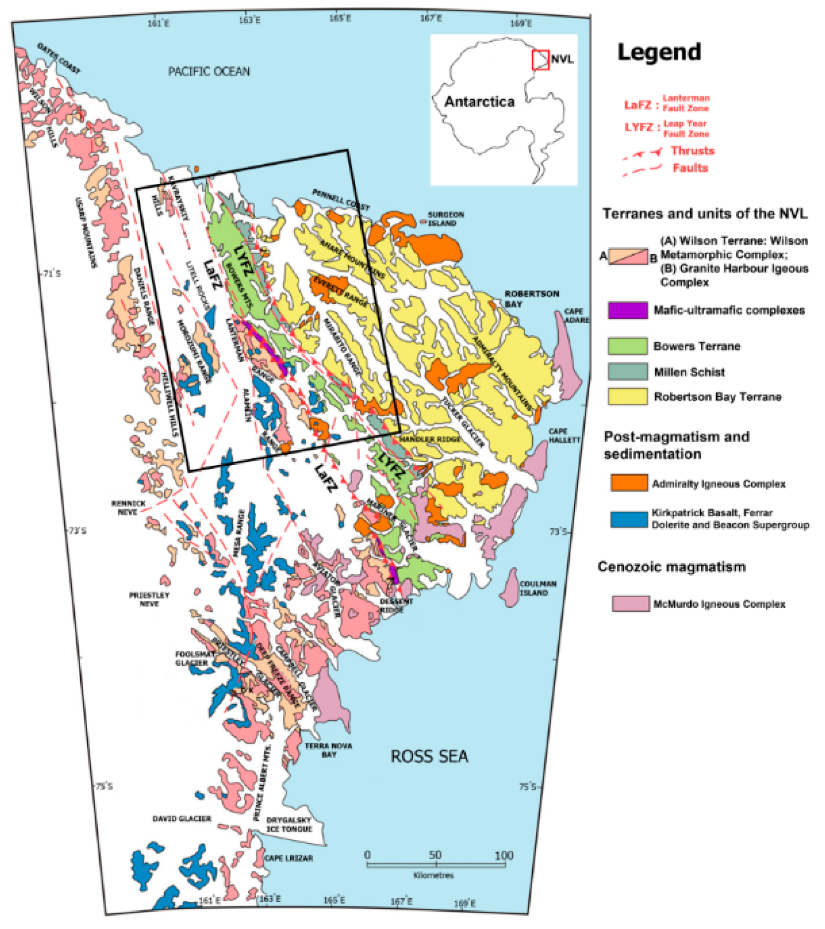
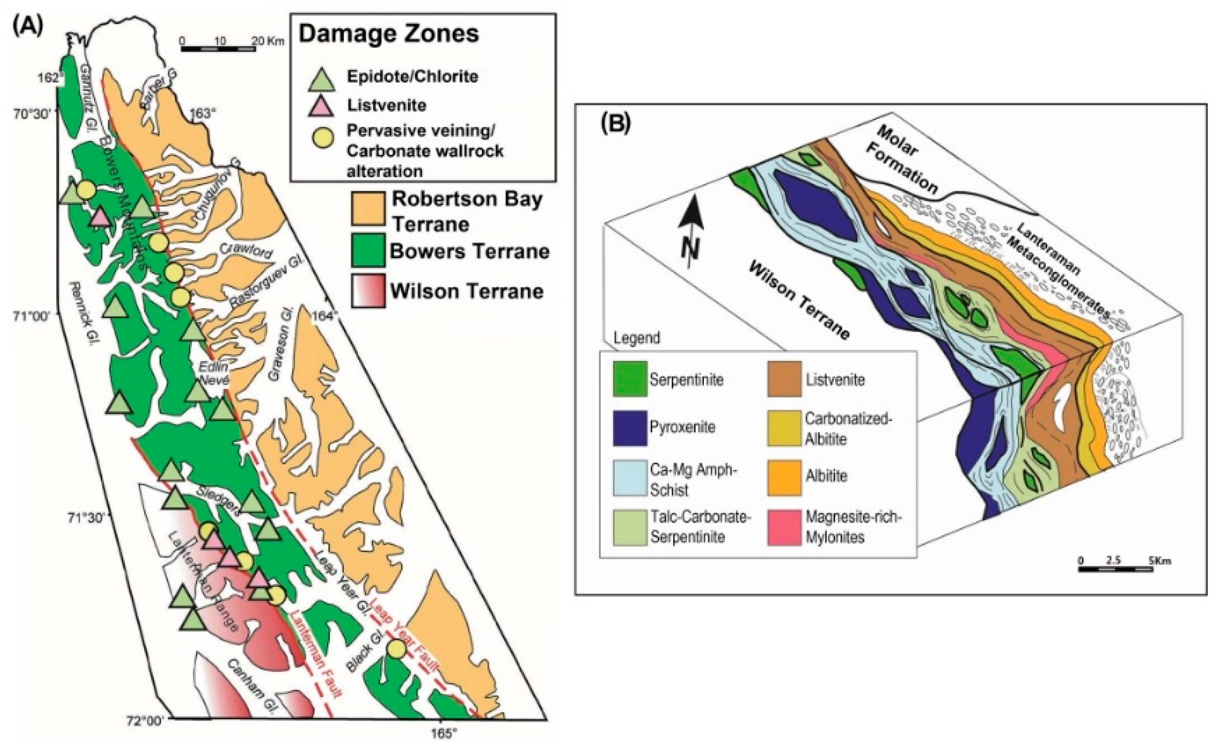
2. Geological Setting of NVL and the Bowers Terrane

Northern Victoria Land (NVL) is composed of three NW-trending litho-tectonic units or terranes of late Proterozoic–Ordovician age, which are from west to east (i) the Wilson Terrane (WT), (ii) the Bowers Terrane (BT), and (iii) the Robertson Bay Terrane (RBT) (Figure 1 and Figure 2) [53,54,55]. They are generally interpreted to have formed during west-directed subduction processes at the palaeo-Pacific active continental margin of East Gondwana during the Latest Ediacaran to Early Palaeozoic Ross Orogeny [45]. The WT encompasses polydeformed low- to high-grade (up to granulite facies) metasedimentary sequences intruded by the Granite Harbour Igneous Complex (calc-alkaline plutons with magmatic arc affinity of the latest Ediacaran to Cambro-Ordovician age) [45,56,57,58]. The BT comprises very low-grade to low-grade (prehnite-pumpellyite to lower-greenschist facies) metavolcanic and metasedimentary rocks, which are considered to be an intra-oceanic arc complex [59,60] or a fore-arc volcanic complex at the Ross-orogenic active continental margin [54]. The RBT is a very low- to locally in its western part low-grade (zeolite to prehnite-pumpellyite facies) turbidite sequence, which is interpreted as a synorogenic sedimentary pile in an accretionary environment [61,62,63]. The tectonic boundary between the WT and the BT is generally referred to as the Lanterman Fault Zone (LaFZ), whereas the Leap Year Fault Zone (LYFZ) separates the BT from the RBT by the strongly sheared Millen Schist Belt (Figure 1 and Figure 2) [47,64,65]. These fault zones represent long-lived structures in the structural edifice of NVL, which were repeatedly reactivated [66].

After the Ross orogeny, the three terranes were intruded by Devonian/Carboniferous calcalkaline intrusions (Admiralty Intrusives) and associated felsic volcanics (Gallipoli Volcanics) [67]. A subsequent erosion/exhumation phase produced a regional peneplain surface, on which the Late Carboniferous-Early Jurassic terrestrial sedimentary sequence of the Beacon Supergroup was deposited [68,69]. This was followed by tholeiitic magmatism of late Early Jurassic age (Ferrar Dolerite and Kirkpatrick Basalt) [70]. The Cenozoic tectonics in NVL is predominantly linked to the development of the West Antarctic Rift System (WARS), which involved repeated reactivation of the former Paleozoic discontinuities of the NVL crust [66,71,72]. The Cenozoic transtensional structures influenced the emplacement of alkaline magmatic rocks of the McMurdo Igneous Complex (see Figure 1) [60].

The BT consists of three lithostratigraphic sequences of likely Cambrian to Ordovician in age, including from bottom to top the Sledgers, the Mariner, and the Leap Year groups, respectively [73]. The Sledgers Group includes: (i) the Glasgow Volcanics with basalts, spilites, volcanic breccia and tuffs and (ii) the Molar Formation with sandstone, conglomerate, mudstone and subordinate limestone. The Mariner Group comprises a regressive sequence of shallow marine sandstone, subordinate conglomerate, mudstone and limestone. The Leap Year Group consists of quartz-rich sandstone and conglomerate [74,75,76]. Figure 2B shows a schematic section of the WT-BT boundary, the strip close to the contact with the metaconglomerates on the BT side is characterized by xenolithic blocks of eclogite, amphibolite, serpentinite and listvenite as the main lithologies [77]. The metamorphic grade in the WT ranges from greenschist to amphibolite and up to the granulite facies, which is notably higher and more diverse than the entire BT. In the BT, higher metamorphic grades, including HP metamorphism, are confined only to the proximity of the Lanterman suture zone at the tectonic boundary between the WT and the BT [45,46,78].

3. Materials and Methods

3.1. ASTER Data Characteristics and Pre-processing

Twelve ASTER level 1T (Precision Terrain Corrected Registered At-Sensor Radiance) scenes obtained from U.S. Geological EROS (http://glovis.usgs.gov/) were used for mapping the poorly exposed damage zones of the WT-BT boundary.

Table 1. The dataset characteristics of ASTER images used in this research.

Granule ID	Date and Time of Acquisition	Path/Row	Cloud Coverage	Sun Azimuth	Sun Elevation
AST_L1T_00312282003214501	2003/01/01, 21:45:01	66/110	1%	55.417	34.625
AST_L1T_00301012003215056	2003/01/01, 21:51:05	66/110	2%	56.520	34.555
AST_L1T_00301012003215105	2003/01/01, 21:51:05	66/111	1%	56.972	34.077
AST_L1T_00301012003215114	2003/01/01, 21:51:14	66/111	1%	57.568	33.573
AST_L1T_00301192003213854	2003/01/19, 21:38:54	66/111	3%	61.896	29.830
AST_L1T_00301192003213845	2003/01/19, 21:38:45	66/111	1%	61.357	30.402
AST_L1T_00312022006215521	2006/12/02, 21:55:21	67/110	1%	52.247	34.707
AST_L1T_00312022006215530	2006/12/02, 21:55:30	67/110	3%	52.693	34.114
AST_L1T_00312022006215539	2006/12/02, 21:55:39	67/111	5%	53.417	33.845
AST_L1T_00301022005221335	2005/01/02, 22:13:35	68/110	1%	52.821	35.641
AST_L1T_00301022005221344	2005/01/02, 22:13:44	68/110	2%	53.395	35.254
AST_L1T_00301022005221353	2005/01/02, 22:13:53	68/111	4%	53.756	35.665

shows the dataset characteristics of the ASTER images used in this research. Atmospheric correction was applied to the ASTER data using Fast Line-of-sight Atmospheric Analysis of Spectral Hypercube (FLAASH) algorithm [79,80], which is available in the ENVI (Environment for Visualizing Images, http://www.exelisvis.com) version 5.2 software package. The Sub-Arctic Summer (SAS) atmospheric and the Maritime aerosol models were used for running the FLAASH algorithm [81]. Crosstalk correction is required before processing of ASTER data to remove the influences of energy overflow from band 4 into bands 5 and 9 [82]. Hence, it was implemented with respect to the ASTER SWIR bands used in this research. The ASTER images were pre-georeferenced to the UTM zone 58 South projection using the WGS-84 datum and rotated to the north up to the UTM projection. Furthermore, the 30-m-resolution SWIR bands were re-sampled to have spatial dimensions of 15 m (corresponding to the VNIR 15-m resolution) using the nearest neighbour re-sampling technique for producing a stacked layer of VNIR+SWIR bands. A masking procedure was used to remove the snow/ice, cloud and shadow by applying the Normalised Difference Snow Index (NDSI) [7,30,83,84]. Radiance at the sensor TIR data without atmospheric corrections was used in this analysis for retaining the original radiance signature. The digital number (DN) value of each pixel in level 1T data at band i (i = 10–14) is linearly converted to radiance registered at the sensor (L_sen) (Wm⁻²·Sr⁻¹·μm⁻¹) [41,42], by the application of Equation (1):

$${\mathrm{L}}_{\mathrm{sen}}^{\mathrm{i}}={\mathrm{cof}}^{\mathrm{i}}\times ({\mathrm{DN}}^{\mathrm{i}}-1)$$

(1)

where, cof¹⁰ = 0.006882, cof¹¹ = 0.006780, cof¹² = 0.006590, cof¹³ = 0.005693, and cof¹⁴ = 0.005225.

3.2. Image Processing Algorithms

Spectral information for detecting alteration mineral assemblages and listvenites in the damage zones of the WT-BT boundary were extracted at pixel and sub-pixel levels using specialized/standardized image processing algorithms. For regional-scale mapping of the WT-BT boundary, pixel-based algorithms, including Principal Component Analysis (PCA) and Independent Component Analysis (ICA) were used. Sub-pixel-based algorithms, namely Linear Spectral Unmixing (LSU) and Constrained Energy Minimization (CEM), were applied for detailed mapping in some selected subsets of the damage zones at local scale. Figure 3 shows an overview of the BT and surrounding area (the coverage of ASTER images used in this study), along with six selected subsets of the fault zones (zones 1–6) for detailed mineral mapping. A flowchart of the methodology used in this research is shown in Figure 4. For processing the datasets, the ENVI (Environment for Visualizing Images, http://www.exelisvis.com) version 5.2 and ArcGIS version 10.3 (Esri, Redlands, CA, USA) software packages were used.

3.2.1. Spectral Information Extraction at the Pixel Level

A fusion of PCA and ICA algorithms was implemented to the ASTER VNIR+SWIR and TIR datasets for extracting image spectra at the pixel level to map poorly exposed lithologies and alteration mineral assemblages. The PCA technique selects uncorrelated linear combinations (Eigenvector loadings) of variables in such a way that each component successively extracted linear combination and contains a smaller variance [85,86,87,88]. The Eigenvector loadings contain important information for identifying hydrothermal/metasomatic alteration mineral assemblages. By computing the correlation of each band k with each component p, it is possible to determine how each band “loads” or are associated with each principal component (Equation (A1), see Appendix A) [86].

A PC image with moderate to high eigenvector loading for the indicative bands (reflection and/or absorption bands) of the mineral with opposite signs enhance that mineral [89]. If the loading is positive in the reflection band of the mineral, the enhanced pixels related to the mineral will manifest as bright pixels. On the contrary, if the loading is negative in the reflection band of the mineral, the enhanced pixels related to the mineral will manifest as dark pixels [90]. Consequently, eigenvector loadings in each PCA will identify the PC image in which the spectral information of the specific alteration mineral is loaded as bright or dark pixels [91]. The ICA is a statistical and computational technique for array processing and data analysis, aiming at recovering unobserved signals or ‘sources’ from observed mixtures, exploiting only the assumption of mutual independence between the signals [92,93]. It is a method for separating the combinations with the most non-Gaussian possible probability density functions from the more Gaussian signal mixtures [94,95]. These are identified as the “independent components” (ICs) of the observations [96].

For pixel-based image spectra extraction, PCA analysis can remove correlations, but it is not capable of omitting higher-order dependence. However, the ICA removes both correlations and higher-order dependence. Accordingly, a fusion of PCA and ICA has great capability to identify pixels related to poorly exposed lithologies and alteration minerals in the background of extensive snow/ice cover (Antarctic environments). The PCA can be used to give weight to the components and remove the correlation before applying ICA for revealing hidden factors. As a result, this fusion has a great performance to identify the pixels containing the spectral signature of the alteration minerals or mineral groups that are maximally independent of each other. In this study, four spatial subset scenes (include six selected damage zones; see Figure 3) covering exposed lithologies in the WT-BT boundary and intra-BT fault zones in the northern Bowers Mountains were selected for implementing the PCA/ICA fusion technique. The performance characteristics of the technique are summarized in Figure 4. The image eigenvectors were obtained for the PCA analysis using a covariance matrix of VNIR+SWIR and TIR bands (

Table A1. Eigenvector matrix for VNIR+SWIR bands of ASTER. (A): Spatial subset covering zone 1 and surrounding areas; (B): Spatial subset covering zones 2 and 3; (C): Spatial subset covering zone 4 and surrounding areas; and (D): Spatial subset covering zones 5 and 6.

(A)
Eigenvector	Band 1	Band 2	Band 3	Band 4	Band 5	Band 6	Band 7	Band 8	Band 9
PCA 1	0.467805	0.509694	0.512981	0.217468	0.176799	0.246614	0.248711	0.197151	0.134638
PCA 2	−0.300431	−0.288970	−0.263316	0.338230	0.386615	0.342808	0.283244	0.363021	0.404354
PCA 3	0.157609	0.161323	−0.103135	0.006767	0.226125	−0.358278	−0.615519	0.073713	0.612094
PCA 4	0.044681	0.011848	−0.069971	0.090291	−0.633560	−0.438259	0.344247	0.463711	0.240442
PCA 5	0.571038	0.143893	−0.731120	−0.148991	0.161062	0.025766	0.172102	0.073443	−0.186704
PCA 6	0.085901	−0.004662	−0.067071	−0.301431	−0.281197	0.308307	0.264687	−0.553969	0.588366
PCA 7	−0.076892	−0.036997	0.134514	−0.155125	0.497821	−0.618179	0.507327	−0.246778	0.048065
PCA 8	0.068572	0.059992	−0.169358	0.829896	−0.117622	−0.150630	0.013344	−0.485437	−0.044016
PCA 9	0.565673	−0.777720	0.257238	0.065265	0.008201	−0.026038	−0.057528	0.007880	0.024873
(B)
Eigenvector	Band 1	Band 2	Band 3	Band 4	Band 5	Band 6	Band 7	Band 8	Band 9
PCA 1	−0.479262	−0.517939	−0.509952	−0.225048	−0.160278	−0.238705	−0.238099	−0.191397	−0.123923
PCA 2	0.288066	0.267422	0.266615	−0.388911	−0.371102	−0.336818	−0.273033	−0.365435	−0.404865
PCA 3	−0.470308	−0.335548	0.711152	−0.063002	−0.061806	0.155815	0.278307	−0.089651	−0.207174
PCA 4	0.089149	0.081563	−0.378102	0.066965	−0.262842	0.327757	0.541766	0.014714	−0.606397
PCA 5	0.005198	−0.011714	0.013230	−0.289525	−0.571447	−0.297938	0.372870	0.457705	0.389860
PCA 6	−0.143194	0.033396	0.100700	0.637725	−0.213061	−0.346181	−0.285287	0.440341	−0.347880
PCA 7	0.048756	−0.037063	−0.000810	−0.381573	0.612809	−0.398723	0.186662	0.403665	−0.344018
PCA 8	0.019200	−0.050602	0.037382	−0.368910	−0.118495	0.574367	−0.492425	0.505200	−0.133907
PCA 9	−0.659478	0.731979	−0.091948	−0.132052	0.046537	0.019598	−0.007121	−0.002060	0.028260
(C)
Eigenvector	Band 1	Band 2	Band 3	Band 4	Band 5	Band 6	Band 7	Band 8	Band 9
PCA 1	0.436596	0.474941	0.478323	0.259162	0.202467	0.288422	0.293737	0.233995	0.150469
PCA 2	−0.361523	−0.339702	−0.304584	0.341346	0.339529	0.323638	0.270272	0.338853	0.369764
PCA 3	−0.113406	−0.131491	0.013472	−0.038953	−0.199768	0.301020	0.615036	−0.041133	−0.676513
PCA 4	0.646205	0.069871	−0.741104	0.063857	0.083737	0.043079	0.029404	0.011287	−0.119854
PCA 5	−0.081856	0.003684	0.073346	0.258757	0.617458	0.257579	−0.353971	−0.466145	−0.361612
PCA 6	−0.081361	0.054497	0.026637	0.134626	0.188319	−0.340347	−0.252269	0.722429	−0.484494
PCA 7	−0.038421	0.062948	0.062948	0.128723	−0.501280	0.651852	−0.509411	0.194283	−0.050948
PCA 8	0.065332	−0.071443	0.035478	−0.833862	0.356670	0.335182	−0.066825	0.222638	0.021186
PCA 9	−0.478726	0.790450	−0.345997	−0.117250	0.039925	0.012703	0.092941	−0.045796	0.007618
(D)
Eigenvector	Band 1	Band 2	Band 3	Band 4	Band 5	Band 6	Band 7	Band 8	Band 9
PCA 1	0.457469	0.496121	0.484720	0.241961	0.190767	0.264428	0.267634	0.222557	0.153665
PCA 2	−0.318221	−0.311611	−0.309208	0.348166	0.377922	0.352360	0.263388	0.321127	0.381217
PCA 3	0.050573	0.100867	0.065376	−0.074127	0.348897	−0.190996	−0.603883	−0.184339	0.648564
PCA 4	−0.576526	−0.199530	0.760114	−0.121149	−0.074678	−0.014245	0.117300	−0.037045	0.120188
PCA 5	0.062048	0.065969	−0.120679	−0.198503	−0.582283	−0.293206	0.201001	0.452767	0.517116
PCA 6	0.076383	0.014735	−0.110901	−0.152342	−0.282329	0.477741	0.275588	−0.676196	0.342499
PCA 7	0.082735	−0.021608	−0.059222	−0.230230	0.454540	−0.555810	0.600908	−0.236367	0.060691
PCA 8	0.018744	0.033687	−0.043334	−0.827212	0.260085	0.381570	−0.039539	0.303178	−0.075067
PCA 9	−0.581066	0.774987	−0.234825	0.012884	0.021499	−0.022616	0.039495	−0.044352	−0.044133

;

Table A2. Eigenvector matrix for TIR bands of ASTER. (A): Spatial subset covering zone 1 and surrounding areas; (B): Spatial subset covering zones 2 and 3; (C): Spatial subset covering zone 4 and surrounding areas; and (D): Spatial subset covering zones 5 and 6.

(A)
Eigenvector	Band 10	Band 11	Band 12	Band 13	Band 14
PCA 1	−0.387065	−0.400716	−0.418903	−0.501105	−0.512857
PCA 2	0.124757	−0.148619	−0.793719	0.106037	0.566669
PCA 3	−0.639764	−0.511314	0.328506	0.186276	0.432023
PCA 4	0.630731	−0.744700	0.169973	0.079875	−0.111041
PCA 5	0.165821	0.036321	0.240257	−0.834608	0.465714
(B)
Eigenvector	Band 10	Band 11	Band 12	Band 13	Band 14
PCA 1	−0.393525	−0.404088	−0.412766	−0.496019	−0.515209
PCA 2	0.068174	0.244757	0.733503	−0.274307	−0.567605
PCA 3	−0.739002	−0.349952	0.467340	0.209083	0.263226
PCA 4	−0.528835	0.806255	−0.213160	−0.138353	0.075548
PCA 5	0.121244	−0.065522	0.166595	−0.784770	0.580852
(C)
Eigenvector	Band 10	Band 11	Band 12	Band 13	Band 14
PCA 1	−0.387916	−0.409696	−0.430823	−0.491519	−0.504450
PCA 2	0.059723	0.202526	0.734577	−0.249602	−0.594568
PCA 3	−0.749770	−0.351003	0.439774	0.248107	0.244302
PCA 4	0.532694	−0.814304	0.224886	0.010234	0.049680
PCA 5	−0.006039	0.069557	0.175536	−0.796521	0.574340
(D)
Eigenvector	Band 10	Band 11	Band 12	Band 13	Band 14
PCA 1	−0.386572	−0.407245	−0.432094	−0.491312	−0.506577
PCA 2	0.007595	−0.170349	−0.765517	0.204563	0.585714
PCA 3	0.667689	0.466491	−0.419996	−0.168193	−0.363168
PCA 4	0.605752	−0.766295	0.140070	0.132069	−0.093781
PCA 5	0.194321	-0.017612	0.176809	−0.819167	0.509541

, see Appendix A). Subsequently, a forward ICA rotation was applied to the PCs images (see Figure 4). The IC images were statistically examined for each of the selected spatial subset scenes (Table A1 and Table A2, see Appendix A). The ICs contain maximally independent pixels of alteration minerals or mineral groups were selected to produce Red-Green-Blue (RGB) color composite image maps.

3.2.2. Spectral Information Extraction at the Sub-pixel Level

The LSU and CEM algorithms were applied to VNIR+SWIR bands for detailed mapping of alteration minerals and listvenites at the sub-pixel level in the six selected subsets of fault zones (see Figure 3). The LSU is a sub-pixel sampling algorithm [97,98,99], the reflectance at each pixel of the image is assumed to be a linear combination of the reflectance of each material (or end-member) present within the pixel. The LSU is used to determine the relative abundance of end-members within a pixel based on the end-members’ spectral characteristics. In this algorithm, it is assumed that the observed pixel reflectance can be modeled as a linear mixture of individual component reflectance multiplied by their relative proportions. Mathematically, the LSU can be represented as Equation (A2) [100] (see Appendix A).

In this study, the Automated Spectral Hourglass (ASH) technique [81,101,102] was employed to extract reference spectra directly from the ASTER image for producing fraction images of end-members using the LSU. The ASH technique uses the spectrally over-determined data for finding the most spectrally pure pixels (end-members) to map their locations and estimates their sub-pixel abundances [81]. It includes several steps, namely: (i) the Minimum Noise Fraction (MNF) [103,104]; (ii) the Pixel Purity Index (PPI) [105]; and (iii) automatic end-member prediction from the n-Dimensional Visualizer [104,106]. The performance characteristics of MNF, PPI and the n-D Visualizer used in this study are shown in Figure 4. The continuum-removal process was applied to the extracted end-members for isolating their spectral features and putting them on a level playing field so they may be intercompared. Continuum-removal and feature comparison is the key to successful spectral identification [34,107,108].

The CEM is a target detection algorithm [109,110,111] that implements a partial unmixing of spectra to estimate the abundance of user-defined end-member materials from a set of reference spectra (either image or laboratory spectra) [112]. It specifically constrains the desired target spectra using a Finite Impulse Response (FIR) filter [113,114], while minimizing effects caused by unknown background signatures [115,116]. Mathematical details of the CEM performance can be found in Chang et al. [112] and Manolakis et al. [111]. For running the CEM, only prior knowledge of desired target spectra (end-member materials) is needed. In this study, the reference spectra of some hydrothermal alteration minerals (typically associated with listvenites) were selected from the USGS spectral library (version 7.0; [117]) for executing the CEM. The performance characteristics of the CEM are summarized in Figure 4. End-member spectra of goethite, hematite, jarosite, biotite, kaolinite, muscovite, antigorite, serpentine, talc, actinolite, chlorite, epidote, calcite, dolomite, siderite and chalcedony were selected and convolved to response functions of ASTER VNIR+SWIR bands (Figure 5). The end-member spectra of the target minerals were used to generate fraction images of prospective alteration minerals associated with listvenites in the poorly exposed fault zones along the WT-BT boundary and intra-BT fault zones in the northern Bowers Mountains.

3.3. Fieldwork Data and Laboratory Analysis

Different locations of exhumed fault systems that are systematically associated with hydrothermal alterations in the poorly exposed damage zones along the WT-BT and BT-RBT boundaries, as well as along major faults and shear zones within the BT and in the easternmost WT along the Rennick Glacier, were investigated. Geological field work was performed during various Italian (PNRA) and German Scientific Expeditions (GANOVEX) in Northern Victoria Land (NVL) and was particularly conducted at several major outcrop sites in the Lanterman Range area, the Molar Massif, and the Bowers Mountains, the Explorers Range on the Rennick Glacier side to the western part facing the Lillie Glacier. Locations of alteration zones and listvenites were recorded using a Garmin Montana 608t handheld GPS with an average accuracy of 5 m and an iPhone SE using GPS plus GLONASS (

Table A3. Locations of alteration zones and listvenites recorded by Global Positioning System (GPS) readings.

Altered Rock Types	Coordinates
Listvenites	71°36.026′S–163°16.302′E
Listvenites	71°36.011′S–163°16.364′E
Carbonitization	70°47.459′S–162°39.438′E
Carbonitization	70°47.349′S–162°38.688′E
Listvenites + sulfides+ albitites	71°33.638′S–163°11.716′E
Epidotization + fault zone	71°23.702′S–162°47.968′E
Reddish to greenish alteration zone	71°19.056′S–162°35.167′E
Epidotization + chlorite in granitoids	71°31.135′S–162°59.086′E
Epidotization + prehnite in granite	71°49.569′S–161°18.145′E
Epidotization + prehnite in granite	71°29.123′S–162°38.567′E
Epidotization in granite	71°44.753′S–162°59.358′E
Epidote + serpentine + talc in high grade mafic-ultramafic rocks	71°27.635′S–162°53.098′E
Listvenite + serpentine in ultramafic rocks	71°34.546′S–163°11.185′E
Listvenite + carbonates in volcanoclastic rocks	71°32.738′S–163°31.602′E
Listvenite + carbonates + talc	71°36.768′S–163°16.407′E
Carbonitization + silica in volcanoclastic rocks	71°33.075′S–163° 31.949′E
Epidotization in Glasgow Volcanics	71°11.159′S–163°00.378′E
Epidote + prehnite + quartz in volcanoclastic rocks	71°23.048′S–162°48.796′E
Listvenite + quartz + hydraulic breccia in Glasgow Volcanics	71°27.078′S–163°26.689′E
Epidote coating fault in Glasgow Volcanics	71°11.292′S–162°35.369′E
Listvenites in ultramafic rocks	71°38.525′S–162°24.458′E

, see Appendix A). Field photos were taken of exposed lithologies, hydrothermally fault-bounded altered rocks and listvenites occurrences during most recent expeditions (2015–2016 and 2016–2017 summer season) and several rock samples were also collected for laboratory analysis. The rock samples were examined by optical microscopy of thin sections and investigated by X-ray diffraction (XRD) analysis for determining their mineralogical composition. Mineral phases were investigated by a Philips PW3710 X-Ray diffractometer (current: 20 mA, voltage: 40 kV, range 2θ: 5–80°, step size: 0.02° 2θ, time per step: 2 s) at DISTAV (University of Genova, Italy), which mounted a Co-anode, as in [49]. Acquisition and processing of the XRD data were carried out using the Philips High Score software package. Additionally, confusion matrix (error matrix) and Kappa Coefficient were calculated for LSU classification mineral maps versus field data (

Table A4. Confusion matrix for LSU classification mineral maps versus field data.

Class	Listvenites	Carbonitization	Epidotization	Totals (Field data)	User’s Accuracy
Listvenites	5	0	1	6	83.33%
Carbonitization	1	5	1	7	71.42%
Epidotization	1	2	5	8	62.50%
Totals (LSU maps)	7	7	7	21
Producer’s Accuracy	71.42%	71.42%	71.42%

Overall accuracy = 71.42%, Kappa Coefficient = 0.57

, see Appendix A).

4. Results

4.1. Regional Overview of the BT and Surrounding Areas

A regional view of the poorly exposed lithological units was generated for the BT and surrounding areas using a mosaic of ASTER images (Figure 6). ASTER Fe-MI = (band 4/band 3) × (band 2/band 1), Al-OH-MI= (band 5 × band 7)/(band 6 × band 6) and Fe, Mg-OH-MI= (band 7 × band 9)/(band 8 × band 8) spectral-band ratio indices [7] were assigned to RGB color composite, respectively. Spatial distribution of iron oxide/hydroxide minerals, Al-OH minerals and Fe,Mg-O-H minerals is manifested by a variety of false color composite in the exposures (Figure 6). Exposed lithologies with a high content of iron oxide/hydroxide minerals are represented as red, magenta and orange colors. The Bowers Mountains and many other parts of the BT and neighbouring areas such as Morozumi Range, Helliwell Hills and Lanterman Range contain a high surface abundance of iron oxide/hydroxide minerals (red, magenta and orange pixels) (Figure 6). Regarding the geological maps of the region, the lithological units in these zones mostly consist of the Wilson Terrane metamorphic rocks, Granite Harbour Igneous Complex, metavolcanic rocks (Glasgow Volcanics), Admiralty Intrusives, Ferrar Dolerite and Kirkpatrick Basalt.

Most of the sedimentary rock units in the study area comprise the Beacon Supergroup, Robertson Bay Group, Molar Formation, Mariner Group and Leap Year Group, which appear in green and blue colors (Figure 6). Generally, sedimentary rocks contain large amounts of Al-OH and Fe,Mg-O-H mineral assemblages (detrital clay minerals). Very poorly exposed outcrops adjacent to the Morozumi Range, Helliwell Hills and ANARE Mountains are represented as cyan color (Figure 6). The exposures in the central part of the Mirabito Range, the southern part of the Alamein Range and the central-northern part of the Everett Range are depicted as yellow color (Figure 6). This indicates that these exposures mostly contain iron oxide/hydroxide minerals in association with Al-OH minerals. Some of the exposed rocks in the southern and western parts of the Mirabito Range and the northern part of the ANARE Mountains are manifested in purple color (Figure 6) due to the admixture of iron oxides/hydroxides with Fe,Mg-O-H mineral groups.

4.2. Alteration and Lithological Mapping in the Fault Zones at Regional Scale

The analysis of the eigenvector matrix for VNIR+SWIR bands (Table A1) and the visual examination of the output IC images indicate the existence of maximally independent pixels related to alteration minerals or mineral groups in some PCAs that contain unique contributions (magnitude and sign of eigenvector loadings) of the minerals. The eigenvector loadings calculated for the spatial subset covering zone 1 and the surrounding areas (Table A1A) reveal that PCA5 has a strong contribution of band 1 (0.571038) and band 3 (−0.731120) with opposite signs. PCA6 shows moderate loadings of band 5 (−0.281197), band 6 (0.308307) and band 7 (0.264687) and strong loadings of band 8 (−0.553969) and band 9 (0.588366), each with opposite signs. PCA7 contains strong weightings of band 5 (0.497821), band 6 (−0.618179) and band 7 (0.507327) with opposite signs, and moderate to low weightings of band 8 (−0.246778) and band 9 (0.048065).

Iron oxide/hydroxide minerals (hematite, goethite, jarosite and limonite) exhibit diagnostic absorption characteristics in band 1 (0.52–0.60 μm), band 2 (0.63–0.69 μm) and band 3 (0.78–0.86 μm) of ASTER [31,118]. The Al-OH minerals (kaolinite, alunite and muscovite) contain absorption features in band 5 (2.145–2.185 μm), band 6 (2.185–2.225 μm) and band 7 (2.235–2.285 μm) of ASTER [119]. On the other hand, the Fe,Mg-O-H and CO₃ minerals (chlorite, epidote and calcite) have distinctive absorption features in band 8 (2.295–2.365 μm) and band 9 (2.360–2.430 μm) of ASTER [120,121]. Accordingly, PCA5, PCA6 and PCA7 have great potential to hold maximally independent pixels related to iron oxide/hydroxide minerals, Al-OH minerals and Fe,Mg-O-H and CO₃ minerals, which can be specifically revealed using ICA analysis. Examination of the Z-Profiles (interactively plot the spectrum for the pixel under the cursor [81]) of the output IC images indicated that the identified pixels are independently and spectrally related to the indicated minerals.

PCA5, PCA7 and PCA6 were assigned to the RGB color composite for mapping iron oxide/hydroxide minerals, Al-OH minerals and Fe,Mg-O-H and CO₃ minerals, respectively. Figure 7A shows the resultant image map for the spatial subset covering zone 1 and the surrounding areas. Magenta, red, yellow and light yellow pixels predominate in the exposed zones, and green and blue pixels are less in abundance (Figure 7A). Thus, iron oxide/hydroxide minerals have high surface abundance in the exposed lithologies in zone 1. However, Al-OH minerals and Fe,Mg-O-H and CO₃ mineral assemblages have low surface abundance and are generally associated with iron mineral groups as magenta, yellow and light yellow pixels. With reference to the geological map of zone 1 and the surrounding areas, the exposed lithological units mostly consist of Wilson Terrane metamorphic rocks, Granite Harbour Igneous Complex, Beacon Supergroup and Ferrar Dolerite. Surface distribution of iron oxide/hydroxide minerals (red and magenta pixels) is typically associated with the Ferrar Dolerite and Granite Harbour Igneous Complex (Figure 7A), for instance, the exposures of Ferrar Dolerite in the northern part of the Alamein Range and the exposed zones of the Granite Harbour Igneous Complex along the Hunter Glacier in the southern part of the Lanterman Range. The Al-OH and Fe,Mg-O-H and CO₃ minerals (green, blue, yellow and light yellow pixels) are mainly concentrated in exposures of the Beacon Supergroup and Wilson Terrane metamorphic rocks (particularly amphibolite-facies metasedimentary rocks).

Table A1B shows the eigenvector loadings for the spatial subset covering zones 2 and 3. PCA3 shows strong contributions of band 1 (−0.470308) and band 3 (0.711152) with opposite signs. PCA6 contains strong loadings of band 8 (0.440341) and band 9 (−0.347880) with opposite signs. PCA7 has strong to moderate contributions of band 5 (0.612809), band 6 (−0.398723) and band 7 (0.186662) with opposite signs, and strong loadings of band 8 (0.403665) and band 9 (−0.344018). Considering the eigenvector loadings in PCA7, this PCA contains the contribution of both Al-OH and Fe,Mg-O-H and CO₃ mineral groups. ICA rotation is able to separate maximally independent pixels related to two different mineral groups. Therefore, PCA3, PCA7 and PCA6 were selected for ICA rotation and subsequent generation of an RGB color composite to detect iron oxide/hydroxide, Al-OH and Fe,Mg-O-H and CO₃ minerals, respectively. Figure 7B displays the resultant image map for the spatial subset covering zones 2 and 3. Several types of mineral assemblages are detected. Prevalent distribution of iron oxide/hydroxide minerals (red and magenta pixels) is associated with most of the exposures, while Al-OH minerals (green pixels) and Fe,Mg-O-H and CO₃ minerals (blue pixels) are specifically predominant in some exposed zones. The admixture of the mineral groups (yellow and cyan pixels) is also observable in some small exposures (Figure 7B). Comparison with the geological map of the study zones indicates that iron oxide/hydroxide minerals are typically associated with exposures of the Granite Harbour Igneous Complex of the WT, Glasgow metavolcanic rocks of the BT, Robertson Bay Group of the RBT and Admiralty Intrusives. The Al-OH minerals and Fe,Mg-O-H and CO₃ minerals characterize the exposed zones of metasedimentary rocks (the Molar Formation, Mariner Group and Leap Year Group) of the BT, Wilson Terrane metamorphic rocks and Ferrar Dolerite.

Considering eigenvector loadings for the spatial subset covering zone 4 and surrounding areas (Table A1C), it is evident that PCA4, PCA5 and PCA6 contain spectral information to identify iron oxide/hydroxide, Al-OH and Fe,Mg-O-H and CO₃ mineral groups at the pixel level. PCA4 shows strong weightings of band 1 (0.646205) and band 3 (−0.741104) with opposite signs. PCA5 has strong to moderate contributions of band 5 (0.617458), band 6 (0.257579) and band 7 (−0.353971) with opposite signs. PCA6 contains strong loadings of band 8 (0.722429) and band 9 (−0.484494) with opposite signs (Table A1C). Therefore, the ICA rotation and subsequent RGB color composite were applied to PCA4, PCA5 and PCA6 for mapping the iron oxide/hydroxide, Al-OH and Fe,Mg-O-H and CO₃ mineral groups, respectively. Figure 7C displays the resultant image map for the spatial subset covering zone 4 and the surrounding areas. The iron oxide/hydroxide mineral group appears as red and magenta color pixels, which mainly predominate in exposed lithologies associated with the Litell Rocks region (consists of Kirkpatrick Basalts/Ferrar Dolerite) in the south-western part of the image. The Al-OH mineral group is represented as green and cyan color pixels, which are associated with exposed rocks in the Bowers Mountains (Figure 7C). Conceivably, they are exposures of the Molar Formation and the Mariner Group that contain a high content of clay minerals. The Fe,Mg-O-H and CO₃ minerals manifest in blue color pixels, which have low surface abundance in the study zone. However, they are generally associated with iron oxide/hydroxide minerals in several exposed zones (Figure 7C). The exposures could possibly contain a high content of Fe,Mg-O-H and iron oxide/hydroxide minerals in the Bowers Mountains are Glasgow metavolcanic rocks of the BT. The Autobahn Moraine is a prominent and linear large moraine stretching over several 10s of kilometres along the Rennick Glacier [122]. The iron oxide/hydroxide and Al-OH mineral groups are mapped in the Autobahn Moraine (the central part of Figure 7C).

Analysing the eigenvector loadings for the spatial subset covering zones 5 and 6 (Table A1D) indicate that PCA4 has strong contribution of band 1 (−0.576526) and band 3 (0.760114), PCA6 contains strong loadings of band 8 (−0.676196) and band 9 (0.342499) and PCA7 shows strong weightings of band 5 (0.454540), band 6 (−0.555810) and band 7 (0.600908). Thus, PCA4, PCA7 and PCA6 were selected for the ICA rotation and were subsequently assigned to an RGB color composite for identifying iron oxide/hydroxide, Al-OH and Fe,Mg-O-H and CO₃ mineral groups. Figure 7D shows the resultant image map for the spatial subset covering zones 5 and 6, which covers the Bowers Mountains, Millen Schist and Robertson Bay Terrane (RBT) from west to east. Magenta, red, yellow and green pixels govern most of the exposures, while blue pixels are much less abundant. Hence, iron oxide/hydroxide and Al-OH mineral groups and their admixture are dominant mineral assemblages in the study zone. The Glasgow Volcanics, the Molar Formation, Millen Schist, Robertson Bay Group and Admiralty Intrusives are exposed in zones 5 and 6 with reference to the geological map. It is discernible that the exposures of Glasgow Volcanics and Admiralty Intrusives contain a high surface distribution of iron oxide/hydroxide with some admixture of Al-OH minerals, which appear as magenta, red and yellow pixels in Figure 7D. The Molar Formation, Millen Schist and Robertson Bay Group appear in green color pixels due to the high content of Al-OH mineral assemblages (Figure 7D).

TIR radiation has been stated to be a function of temperature and emissivity [38,123]. In the ASTER TIR dataset, bands 10, 11 and 12 comprise spectral emissivity and temperature information, while in bands 13 and 14, surface temperature dominates the spectral emissivity information [7,123]. Additionally, ultramafic/mafic rocks (gabbro, dolerite and dunite; 40–45% SiO₂) show high spectral emissivity in bands 10 to 12 (8–9 μm) and low emissivity in bands 13 and 14 (10–12 μm), as well as high surface temperature due to low albedos and low thermal inertia [41,42,123,124,125]. Felsic rocks (granite and granitoid; 60–80% SiO₂) show low spectral emissivity in bands 10 to 12 and high emissivity in bands 13 and 14, as well as low surface temperatures attributable to high albedos [41,42,123,124]. In view of this, ASTER TIR bands incorporate maximally independent pixels related to ultramafic-to-mafic, intermediate and felsic lithological units, which can be specifically detected using PCA/ICA analysis.

The analysis of the eigenvector matrix for TIR bands in Table A2 shows unique contributions of eigenvector loadings (magnitude and sign) in some specific PCAs. The Z-Profiles of detected pixels indicate distinctive spectral emissivity features related to different lithological units (ultramafic, mafic, intermediate and felsic rocks) in the output IC images. Table A2A shows eigenvector loadings for the spatial subset of zone 1 and the surrounding areas. PCA2 shows strong contributions of band 12 (−0.793719) and band 14 (0.566669) with opposite signs. PCA3 contains strong loadings of band 10 (−0.639764) and band 11 (−0.511314) with negative signs and band 14 (0.432023) with a positive sign. PCA4 has strong weightings of band 10 (0.630731) and band 11 (−0.744700) with opposite signs. Considering the characteristics appearing in the eigenvector loadings (Table A2A), PCA2 contains maximally independent pixels related to ultramafic-to-mafic units, while PCA3 and PCA4 include the independent pixels of intermediate and felsic units.

The RGB color composite was generated for the zone 1 and the surrounding areas after ICA rotation of PCA2, PCA4 and PCA3 for mapping maximally independent pixels of ultramafic/mafic, felsic and intermediate lithological units, respectively (Figure 8A). The image map contains red, magenta, yellow, light yellow and green pixels. Comparison with the geological map indicates that red and magenta pixels generally match the Wilson Terrane metamorphic rocks and Ferrar Dolerite, which are composed of ultramafic-to-mafic lithological units. The yellow and light yellow pixels match well with exposures of the Granite Harbour Igneous Complex (Figure 8A). The green pixels match the Beacon Supergroup (arkosic quartz sandstone). The intermediate trend can be expected with the quartz-rich/feldspar-rich rocks (granite and granitoid), while the felsic trend is correlated with quartz-rich rocks (quartzose sedimentary rocks) due to the high content of SiO₂ and spectral property of quartz [42,124].

Based on the eigenvector loadings for the spatial subset of zones 2 and 3 (Table A2B), PCA2 shows strong positive loading of band 12 (0.733503) and strong negative loading of band 14 (−0.567605); PCA3 contains strong negative contribution of band 10 (−0.739002) and strong positive contribution of band 12 (0.467340); and PCA4 has strong negative weighting of band 10 (−0.528835) and strong positive weighting of band 11 (0.806255). Hence, PCA2, PCA3 and PCA4 images comprise maximally independent pixels related to ultramafic-to-mafic, intermediate and felsic lithological units, respectively. These PCA images were selected for ICA rotation and a false-color composite image map was generated by allocating red color to ultramafic-to-mafic rocks (the ICA2 image), green color to felsic rocks (the ICA4 image) and blue color to intermediate rocks (the ICA3 image) (Figure 8B). Green, cyan, yellow and red color pixels are depicted in the image map. Yellow pixels refer to combined mafic and felsic trends, while cyan pixels contain felsic in the intermediate signature. With reference to the geological map of the study area, red pixels are mainly associated with exposures of the Glasgow metavolcanic rocks of the BT and Ferrar Dolerite; yellow pixels are mostly considered with exposed zones of the Granite Harbour Igneous Complex and Wilson Terrane metamorphic rocks; green and cyan pixels are generally represented in the exposures of metasedimentary rocks (the Molar Formation, Mariner Group and Leap Year Group) of the BT, Robertson Bay Group and Admiralty Intrusives.

Table A2C shows the eigenvector matrix for the spatial subset covering zone 4 and the surrounding areas. PCA2 has high eigenvector loadings in band 12 (0.734577) and band 14 (−0.594568) with opposite signs. PCA3 shows a strong negative contribution of band 10 (−0.749770) and strong positive contribution of band 12 (0.439774). PCA4 contain strong positive loading of band 10 (0.532694) and high negative loading of band 11 (−0.814304). After ICA rotation, red, green and blue colors were used to produce a false-color composite image map of the ICA2 (ultramafic-to-mafic rocks), ICA4 (felsic rocks) and ICA3 (intermediate rocks). Figure 8C shows the resultant image map for zone 4 and the surrounding areas. Green, cyan, blue and red color pixels are observable. The concentration of red pixels mostly corresponds with the Litell Rocks region (Ferrar Dolerite) and Glasgow metavolcanic rocks, while green and cyan pixels are likely associated with metasedimentary rocks (Molar Formation, Mariner Group and Leap Year Group) of the BT. Blue pixels are probably the admixture of the metavolcanic and metasedimentary rocks in the Bowers Mountains, which show an intermediate trend in the image map (Figure 8C). The green, red and magenta pixels that appear as long linear/curve patterns in the central part of the image (corresponding with the Rennick Glacier) seem to be the Autobahn Moraine [122].

Considering the eigenvector loadings for the spatial subset covering zones 5 and 6 (Table A2D), PCA2 shows high weighting with a negative sign in band 12 (−0.765517) and great contribution with a positive sign in band 14 (0.585714). PCA3 has strong loading of band 10 (0.667689) and band 12 (−0.419996) with opposite signs. PCA4 contains a strong contribution of band 10 (0.605752) with a positive sign and high loading of band 11 (−0.766295) with a negative sign. The ICA rotation was applied to PCA2, PCA3 and PCA4. Accordingly, the ICA2, ICA4 and ICA3 were assigned to RGB false-color composite for mapping ultramafic-to-mafic rocks, felsic rocks and intermediate rocks, respectively. Figure 8D shows the resulting image map of the selected zone. Red and magenta pixels are mainly associated with the exposure of the Glasgow Volcanics, which are mainly mafic in composition. Yellow pixels with an intermediate composition likely correspond to the exposed zones of Admiralty Intrusives and the admixture of the metasedimentary and metavolcanic rocks of the Bowers Mountains. Green and cyan pixels reflect felsic lithologies that typically characterize the Molar Formation, Millen Schist and Robertson Bay Group exposures (Figure 8D).

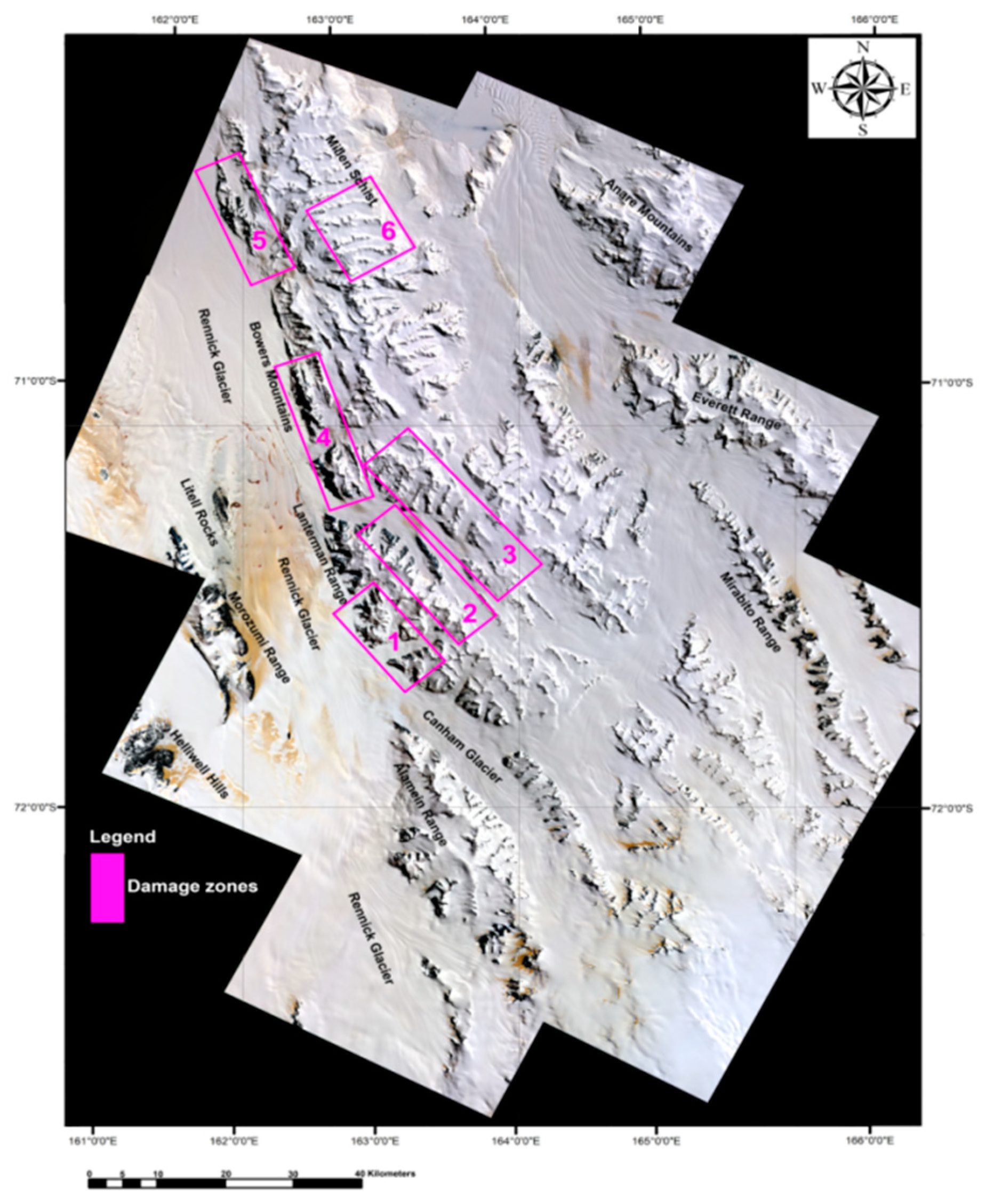
4.3. Detection of Hydrothermal Alteration Minerals and Prospecting Listvenites in the Selected Subset of Damage Zones

The LSU and CEM algorithms were used for sub-pixel level mapping of alteration mineral assemblages and prospecting listvenites in the six selected subsets of damage (fault) zones (zones 1–6) (see Figure 3). A set of unique pixels (corresponding to a pure end-member) was defined using the n-Dimensional analysis technique for each selected subset. Figure 9 shows end-member (mean) spectra extracted for each selected subset of the six study zones. Subsequently, end-member spectra extracted for each selected subset from the apparent reflectance data were used to act as end-members for LSU spectral mapping. Comparison with selected end-member reflectance spectra of minerals from the USGS spectral library that resampled to response functions of ASTER VINR+SWIR bands (see Figure 5) indicates that the extracted end-members or a subset of the extracted end-members can be considered for LSU classification.

The spectral patterns are classified based on the relative absorption intensities. The most dominant spectral patterns often characterize the most abundant minerals (spectrally dominant species) in the rock, which could also be influenced by subordinate phases (spectrally less active or less abundant groups). Generally, in a mineral mixture or association, the identification of different mineralogical phases is complicated when more than one spectrally active mineral group is present [126]. As a result, the extracted end-member spectra for the study zones could be classified to seven spectrally active groups based on Fe²⁺, Fe³⁺, Fe-OH, Al-OH, Mg-OH and CO₃ spectral absorption features, namely (i) goethite/hematite/jarosite group; (ii) kaolinite group; (iii) biotite/muscovite group; (iv) chlorite/epidote/actinolite group; (v) serpentine/antigorite/talc group; (vi) calcite/dolomite/siderite group; and (vii) unaltered/unknown mineral group.

Figure 9A shows extracted end-member spectra for the subset zone (1). Some obvious distinctions between spectral signatures for a variety of minerals are recognizable especially for iron oxide/hydroxide, kaolinite and biotite/muscovite groups. n-D class #1, n-D class #2, n-D class #8, n-D class #9 and n-D class #10 typically represent iron oxide/hydroxide absorption characteristics. Goethite, hematite and jarosite show strong Fe³⁺ and Fe-OH absorption features at 0.48 μm, 0.83–0.97 μm and 2.27 μm, coinciding with bands 1, 3 and 7 of ASTER, respectively [6,33]. Thus, n-D class #1, n-D class #8 and n-D class #10 can be attributed to jarosite (strong 2.27 μm; Fe-OH absorption) and n-D class #2 and n-D class #9 could be considered for goethite and hematite (0.48 μm and 0.83–0.97 μm; Fe³⁺ absorption) (Figure 9A). n-D class #3 and n-D class #7 can be grouped as unaltered/unknown minerals because these classes do not show any distinctive absorption features related to hydrothermal alteration minerals. n-D class #4 represents biotite due to major Mg,Fe-OH absorption near 2.30 μm and minor Fe³⁺ absorption features at 0.85 μm [108,120], which correspond with bands 3 and 8 of ASTER (see Figure 5D). n-D class #5 exhibits a distinct Al-OH absorption feature at 2.2 μm attributable to muscovite, coinciding with band 6 of ASTER [32,119,121]. n-D class #6 contains Al-OH absorption features of kaolinite at 2.17 μm and 2.2 μm that correspond with bands 5 and 6 of ASTER [33,108,120].

The fraction images of end-members resulting from LSU analysis for zone (1) appear as a series of greyscale rule images, one for each extracted end-member. High digital Number (DN) values (bright pixels) in the rule image represent the subpixel abundance of the target mineral in each pixel and map its location. Considering the resultant fraction images and extracted end-member spectra for zone (1), it is evident that goethite, hematite, jarosite, biotite, muscovite and kaolinite are the dominant minerals. For post classification of the fraction images, the rule image classifier tool was applied using a maximum value option. It should be noted that in spectral mixture analysis, a material with a spectral signature similar, but not identical, to that of an end-member can be modeled along with that end-member and be mapped in that end-member’s fraction image [127]. For that reason, the rule image classifier tool is not capable of assigning all end-member minerals into their different classes. However, spectral signatures different from the background and other minerals can certainly be discriminated and classified. Thus, the red color class was designated for the goethite/hematite/jarosite group, the yellow color class was assigned to the biotite/muscovite group and the green color class was selected for the kaolinite group. The unaltered/unknown mineral group was not considered for post classification in the present study.

Figure 10A shows the LSU classification mineral map for zone (1). The results indicate that zone (1) is spectrally governed by the goethite/hematite/jarosite group, while the biotite/muscovite and kaolinite groups have a smaller contribution to the total mixed spectral characteristics. In zone (1), the Wilson Terrane metamorphic rocks, Granite Harbour Igneous Complex, Beacon Supergroup and Ferrar Dolerite are exposed. Therefore, a high surface abundance of iron oxide/hydroxide minerals is related to the crystal-field transitions of iron ions (Fe⁺² and Fe⁺³) in the primary mafic minerals (olivine, pyroxenes and plagioclase) and/or the alteration of primary mafic minerals within mafic rock units such as the Wilson Terrane metamorphic rocks and Ferrar Dolerite. Kaolinite high abundance zones are mostly associated with the detrital clay minerals of the Beacon Supergroup. The biotite/muscovite group seems to be a phyllic alteration zone associated with the Granite Harbour Igneous Complex. Accordingly, the presence of listvenite bodies in zone (1) is slightly feasible.

Analysis of the extracted end-member spectra for the subset zone (2) (Figure 9B) indicates several distinguishable spectral signatures for the alteration minerals. Hematite, jarosite, kaolinite, biotite, muscovite, actinolite, epidote and chlorite are recognizable (Figure 9B). n-D class #1 shows the spectral characteristics of jarosite and n-D class #2 shows the distinctive absorption features of kaolinite. n-D class #3 represents actinolite due to the iron absorption features in bands 2 and 3, and Mg, Fe-OH absorption in bands 7 and 8 of ASTER (see Figure 5J). n-D class #4 and n-D class #9 lack any distinct spectral features related to the alteration minerals, which can be considered an unaltered/unknown mineral group in zone (2). n-D class #5 and n-D class #8 represent epidote and chlorite because they display a slight iron absorption at 0.85–0.97 μm and a major Mg, Fe-OH absorption at 2.30–2.35 μm [33,108,128], corresponding to bands 2, 3 and 8 of ASTER data, respectively [121]. n-D class #6 and n-D class #7 characterize muscovite and biotite, respectively. n-D class #10 can be considered as mixed spectral features of goethite, hematite and jarosite.

Fraction images of end-members for zone (2) were classified using the rule image classifier tool. The blue color class was assigned for chlorite/epidote/actinolite group and added to the previous classes for producing the LSU classification mineral map. Figure 10B shows the resultant classification map for the subset of zone (2). Goethite/hematite/jarosite and chlorite/epidote/actinolite groups show high surface abundance, whereas kaolinite and biotite/muscovite groups exhibit moderate to less spectral contribution and spatial distribution in zone (2). The association of goethite/hematite/jarosite and chlorite/epidote/actinolite groups is observable with exposures of the Glasgow metavolcanic rocks and metasedimentary rocks (Molar Formation, Mariner Group and Leap Year Group). Kaolinite, biotite/muscovite and iron oxide/hydroxide assemblages are associated with the Granite Harbour Igneous Complex. The Wilson Terrane metamorphic rocks and Ferrar Dolerite exposures are generally dominated by goethite/hematite/jarosite group, while the Beacon Supergroup is governed by kaolinite group. For that reason, listvenite bodies could be located in a zone that spatially contains all of the four alteration mineral assemblages. Please note that the large greenish-colored spot in the area of the Sledgers Glacier is a dense crevasse field, which may contain contamination of clay mineral groups (Figure 10B). Several prospect zones for listvenite bodies are identifiable in zone (2); some of them are delimited by yellow rectangles in Figure 10B.

In zone (3), some spectral signatures related to alteration minerals such as goethite, hematite, jarosite, kaolinite, biotite and muscovite are discernible (Figure 9C). n-D class #1, n-D class #4, n-D class #8 and n-D class #9 can be considered to be an unaltered/unknown mineral group. They do not illustrate any significant absorption features related to the target alteration minerals. n-D class #2 and n-D class #3 represent jarosite. Spectral signatures related to kaolinite, biotite and muscovite are apparent in n-D class #5, n-D class #6 and n-D class #7, respectively. n-D class #10 can be characterized as having mixed spectral features of hematite and goethite. Figure 10C displays the LSU classification mineral map for zone (3). The goethite/hematite/jarosite and biotite/muscovite groups are spectrally predominant. The kaolinite group shows very low surface abundance. Iron oxide/hydroxide and biotite/muscovite mineral groups are concentrated in the exposures of the Glasgow metavolcanic rocks and metasedimentary rocks in the Bowers Mountains. Small exposures of the Granite Harbour Igneous Complex and Admiralty Intrusives contain kaolinite group minerals associated with iron oxide/hydroxide and biotite/muscovite mineral groups, which can be attributed to the alteration products of argillic and phyllic alteration zones. Hence, zone (3) has very low potential for containing listvenites.

Typical spectral signatures for a variety of mineral assemblages are decipherable for zone (4) (Figure 9D). n-D class #1 represents antigorite, which contains Fe³⁺ absorption features and Mg,Fe-OH absorption near 2.30 μm [128,129], coinciding with bands 2, 3 and 8 of ASTER (see Figure 5G). n-D class #2 shows 0.48 μm and 0.83–0.97 μm Fe³⁺ absorption and seems to be a combined spectral signature of goethite and hematite. The unaltered/unknown mineral group can be assigned to n-D class #3. Serpentine shows spectral characteristics related to crystal-field transitions in the Fe²⁺ near 0.4 and 0.5 μm and Fe³⁺ near 0.65 μm and a combination of OH-stretching fundamental with the Al-OH-bending and Fe,Mg-OH-bending modes near 2.20 and 2.30 μm [128,130,131]. Therefore, it seems that n-D class #4 has a serpentine spectral signature, which displays distinctive absorption features in bands 2, 3, 7 and 8 of ASTER (see Figure 5H). n-D class #5 appears to be a combined spectral signature of muscovite and biotite. n-D class #6 is characterized by chlorite and epidote spectral features. n-D class #7 can be considered as a mixed spectral signature for calcite and dolomite. Broad Fe²⁺ absorption features occur in calcite and dolomite spectra near 0.9–1.2 μm and vibrational processes of CO₃ radical cause absorption properties near 2.30–2.35 μm [132,133], which are equivalent to bands 4, 7 and 8 of ASTER. n-D class #8 exhibits siderite due to absorption characteristics related to Fe²⁺, Fe³⁺ and CO₃ in bands 2, 3, 7 and 8 of ASTER (see Figure 5P). n-D class #9 exhibits the kaolinite spectral signature, and n-D class #10 can be considered to be a mixed spectral signature of hematite and jarosite.

Figure 10D shows the LSU classification mineral map for zone (4). Biotite/muscovite, goethite/hematite/jarosite and chlorite/epidote/actinolite mineral groups are spectrally significant and have high surface abundance. However, kaolinite, serpentine/antigorite/talc (cyan color class) and calcite/dolomite/siderite (purple color class) mineral assemblages are weakly distributed in the exposed zones. Since zone (4) covers the Bowers Mountains, biotite/muscovite mineral assemblages (yellow pixels) are likely associated with the Molar Formation and the Mariner Group metasedimentary sequences that contain high contents of detrital clay minerals. Glasgow Metavolcanic rocks contain goethite/hematite/jarosite and chlorite/epidote/actinolite mineral groups because of the alteration of primary mafic mineral within basalts, spilites, volcanic breccia and tuffs. The Autobahn Moraine in the Rennick Glacier [122] is mapped as green pixels in the southwestern part of zone (4) (Figure 4D). Erratic metasedimentary or sedimentary rocks and detritus delivered to this moraine from the Bowers Mountains and/or the Lanterman Range could possibly contain large amounts of kaolinite mineral groups. Zone (4) is a highly likely prospective area for listvenites, where the most of the alteration mineral groups are specifically concentrated and are associated particularly with the Glasgow Volcanics. Some of the prospects in zone (4) are shown by yellow rectangles and circles in Figure 10D.

Deciphering the extracted end-member spectra for zone (5) reveals several distinct spectral signatures for the alteration minerals (Figure 9E). n-D class #1 and n-D class #2 obviously represent chlorite and epidote, respectively. n-D class #3 seems to be the combination of antigorite and talc spectral signatures. Mixed spectra of biotite and muscovite can be seen in n-D class #4. Diagnostic absorption features related to alteration minerals could not be realized in n-D class #5 (unaltered/unknown mineral group). n-D class #6 characterizes actinolite spectral properties. n-D class #7 has the combined spectra of hematite and jarosite. It seems that the spectral signatures of kaolinite are exhibited in n-D class #8. Serpentine, antigorite and talc might display mixed spectral properties in n-D class #9. n-D class #10 represents serpentine. Figure 10E shows the LSU classification mineral map for zone (5). The goethite/hematite/jarosite, kaolinite and serpentine/antigorite/talc mineral groups are considerably predominant. Conversely, biotite/muscovite and chlorite/epidote/actinolite mineral assemblages show low spatial distributions and abundances in this zone. The association of iron oxide/hydroxide, serpentine/antigorite/talc, chlorite/epidote/actinolite mineral assemblages are mostly concentrated in the exposures of Glasgow Volcanics due to the alteration of mafic minerals within meta-basalts, spilites, volcanic breccia and tuffs. Kaolinite is mostly associated with the Molar Formation because of the high content of conglomerate and mudstone. Zone (5) may comprises several listvenite occurrences especially associated with Glasgow Volcanics, where a high surface distribution of serpentine/antigorite/talc group is detected with biotite/muscovite and iron oxide/hydroxide mineral groups. Yellow rectangles and circles show some of the prospective zones (Figure 10E).

Analyzing the spectral signatures related to alteration minerals for zone (6) indicates the presence of goethite, hematite, jarosite, biotite, muscovite, chlorite, actinolite, serpentine and talc (Figure 9F). n-D class #1 shows chlorite. n-D class #2 and n-D class #4 may have mixed spectral signatures related to goethite, hematite and jarosite. n-D class #3 and n-D class #8 do not have any indicative absorption features related to alteration minerals and can be considered an unaltered/unknown mineral group. Biotite and muscovite spectral characteristics can be found in n-D class #5 and n-D class #6, respectively. n-D class #7 represents actinolite. n-D class #9 and n-D class #10 characterize serpentine and talc. The LSU classification mineral map for zone (6) is shown in Figure 10F. Iron oxide/hydroxides (goethite, hematite and jarosite) and chlorite/epidote/actinolite mineral assemblages are spectrally major components, while biotite/muscovite and serpentine/antigorite/talc mineral groups are minor components in this zone. The Glasgow Volcanics show high content of iron oxide/hydroxides minerals, which are locally associated with chlorite/epidote/actinolite, biotite/muscovite and serpentine/antigorite/talc mineral groups. Listvenite bodies could be found in the local association of these mineral assemblages within Glasgow Volcanics exposures in the Bowers Mountains. Several locations could be taken into consideration for listvenite occurrences, some of which are demarcated by yellow rectangles and circles in Figure 10F.

The CEM algorithm was implemented to produce fraction images of selected end-member spectra from the USGS spectral library, including goethite, hematite, jarosite, biotite, kaolinite, muscovite, antigorite, serpentine, talc, actinolite, chlorite, epidote, calcite, dolomite, siderite and chalcedony (see Figure 5). The subset of the zones (2), (4) and (5) was selected for running the CEM because they exhibit a variation of mineral assemblages and several highly likely prospective zones for listvenite occurrences in the LSU classification mineral maps (see Figure 10B,D,E). The spatial subset of zone (2) covering the Lanterman Range and surrounding areas was selected to present in this paper. Fraction images of sixteen selected end-member minerals were produced using the CEM algorithm. Fractional abundance of target end-member minerals appears as a series of greyscale rule images, one for each selected mineral. Pseudo-color ramp of greyscale rule images was generated to illustrate high fractional abundance (high DN value pixels) of the target minerals in zone (2) (Figure 11). This comfortably distinguishes the contrast between subpixel targets and surrounding areas. This contrast expresses the fractional abundance of the target mineral present in the rule image.

Considering Fe²⁺, Fe³⁺, Fe-OH, Al-OH, Mg-OH, Si-OH and CO₃ spectral absorption characteristics of target minerals and the limitations of VNIR+SWIR ASTER spectral bands, seven groups of mineral assemblages could also be discernible here. There might be some confusion for distinctive separation of the absorption features (electronic transitions and molecular vibrational overtones) present in alteration minerals using VNIR+SWIR spectral bands of ASTER, particularly when mixtures occur [134,135]. Therefore, some of the target alteration minerals may have a similar manifestation of the fractional abundances in the CEM rule images. For iron oxide/hydroxide mineral group, fractional abundances of goethite and hematite show almost similar appearance and high mixtures, while jarosite shows low mixtures with them and different spatial fractional abundance in some parts of zone (2) (Figure 11). Examination of the end-member spectra extracted from ASTER VINR+SWIR bands using n-Dimensional analysis for zone (2) indicates the presence of jarosite spectral characteristics as n-D class #1 and mixed spectral features of goethite, hematite and jarosite in n-D class #10 (see Figure 9B). Comparison of the fraction images of biotite and muscovite shows different spatial abundances and low combinations (Figure 11). Looking at the n-Dimensional analysis results for zone (2) shows the identification of spectral signatures for muscovite and biotite in n-D class #6 and n-D class #7, respectively (see Figure 9B).

Fractional abundance of kaolinite exhibits comparable manifestation with the spatial abundance of muscovite in many parts (Figure 11). n-D class #2 derived from n-Dimensional analysis for zone (2) is considered to be kaolinite (see Figure 9B); however, the CEM results indicate that this n-D class can be a mixture of kaolinite and muscovite. Antigorite, serpentine and talc display fractional abundance analogous to actinolite (Figure 11). n-D class #3 extracted from n-Dimensional analysis for zone (2) represents actinolite due to some distinctive spectral signatures (see Figure 9B), which are very similar to spectral features of serpentine/antigorite/talc group (see Figure 5G–J). Hence, there may be some confusion between these minerals when using VINR+SWIR bands of ASTER, and their spectral signatures could appear in only one n-D class (n-D class #3) (see Figure 9B). Fractional abundances of chlorite and epidote show some small spatial differences and high combination. Considering n-D classes for zone (2) (see Figure 9B), n-D class #5 and n-D class #8 are determined to be epidote and chlorite, respectively. Fraction images of calcite, dolomite, siderite and chalcedony exhibit similar spatial abundance and high mixtures with each other, although siderite has a lower distribution in some places (Figure 11). With respect to n-D classes for zone (2) (see Figure 9B), there is a high probability that n-D class #4 can be considered to be the mixed spectral signatures of the calcite/dolomite/siderite group, which was previously considered an unaltered/unknown mineral group in zone (2). Please note that a high degree of spectral contrast is required to distinguish the end-member mineral from the background materials [127]. n-D class #9 (see Figure 9B) might have mixed spectral signatures of chalcedony with other minerals, which was formerly assigned to the unaltered/unknown mineral group in zone (2). This is due to the fact that all mixed-pixel spectra always lie on the line that connects the component spectra [111].

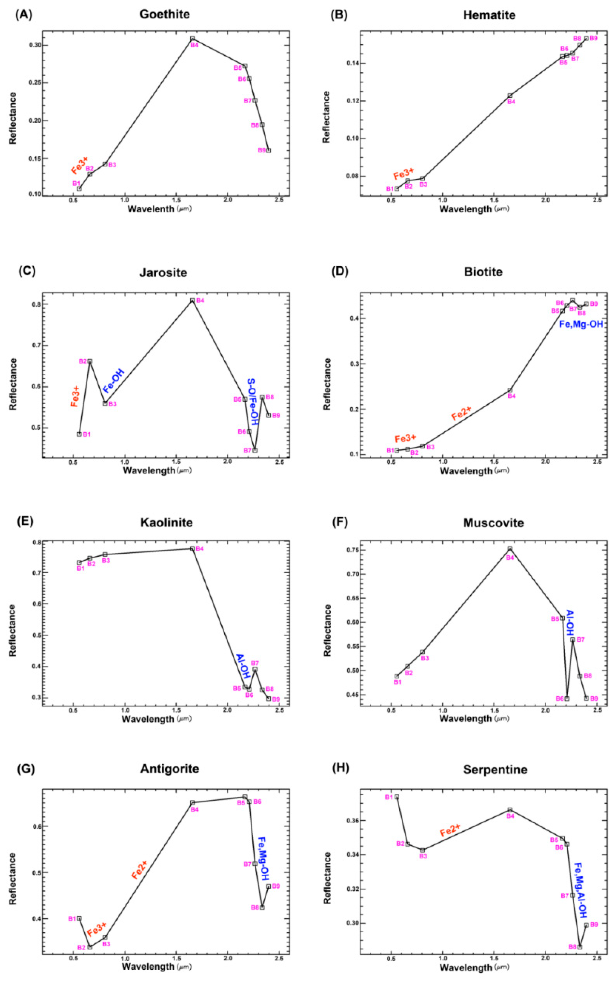
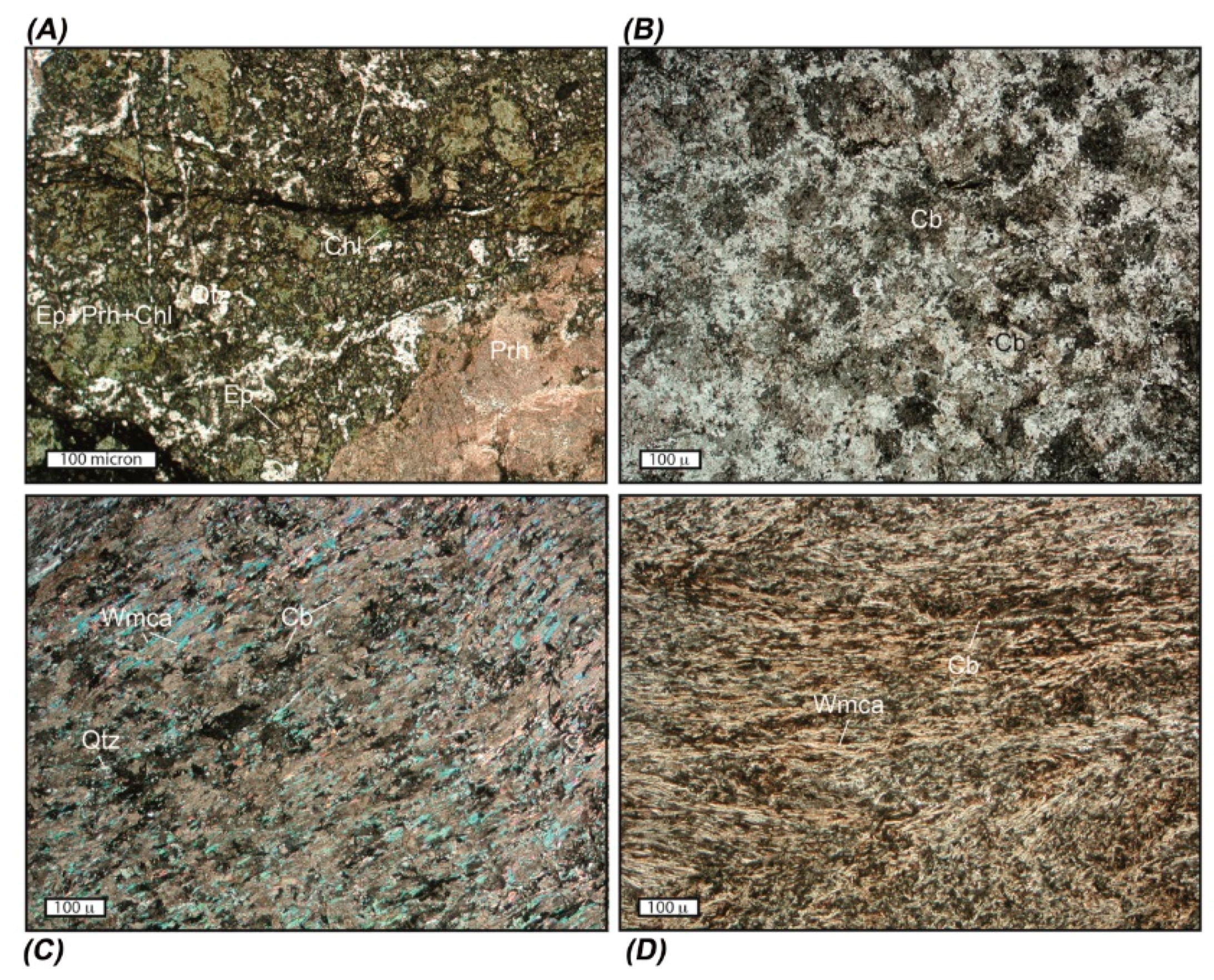
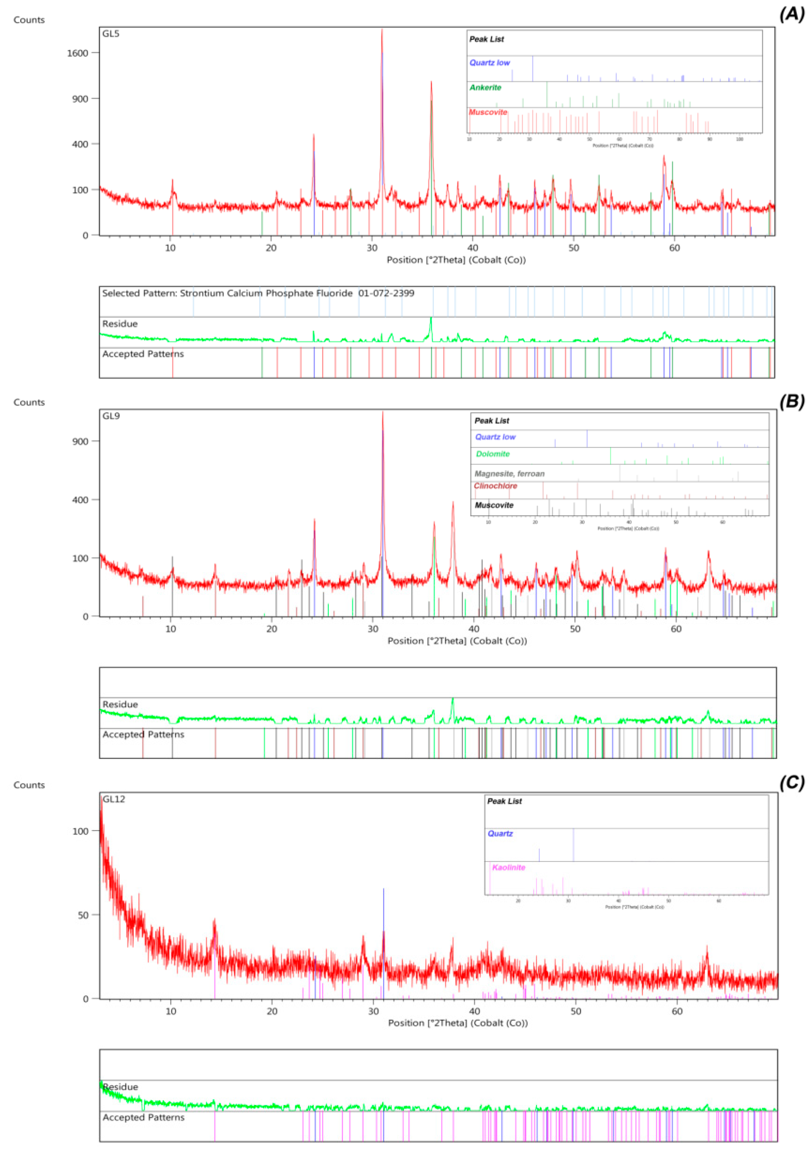
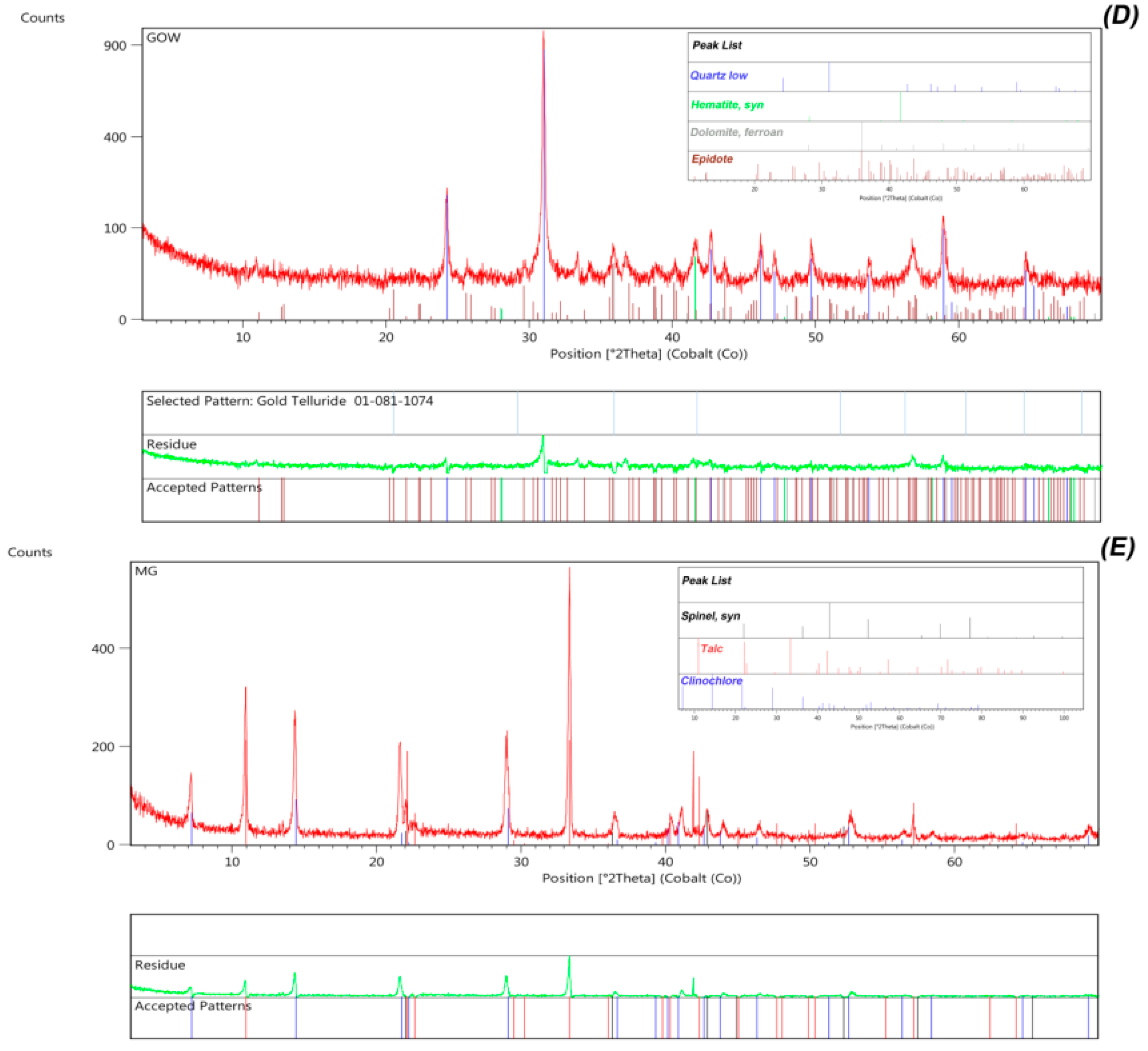
4.4. Petrography and Mineralogy of Hydrothermal Alteration Minerals and Listvenites

Petrographic studies were carried out on samples of hydrothermally altered rocks from the major damage zones of the terrane boundaries and along intra-terrane faults or shear zones. The country rocks comprise low-grade metamorphic basalts and volcaniclastic rocks, low- high-grade metamorphic ultramafic and mafic igneous rocks and granitoids. The observed types of alteration can be divided into the following main groups: (i) Mg-Ca-Fe carbonation and/or silicification of metavolcanic rocks associated with syntectonic carbonate coatings on fault planes, hydraulic brecciation, and quartz-carbonate veining occurring along intra-BT faults and shear zones in the Bowers Mountains and along the BT-RBT boundary damage zone; (ii) epidote-bearing slickensides, epidote veining and epidotization occurring in low-grade metabasalts and in amphibolites in the Lanterman Range and the Bowers Mountains; (iii) epidote-chlorite-prehnite-bearing cataclastites, ultracataclastites, and indurated gouges in fault cores, as well as saussuritization of K-feldspar in the wallrock of granitoid rocks in the western Lanterman Range [136]; (iv) foliated listvenites with Mg-Ca carbonates, quartz, Cr-phengite, Cr-chlorite, magnesite, and talc derived from carbonation of mafic and ultramafic rocks along brittle-ductile shear zones within the WT-BT boundary damage zone and within the BT [1,137] (see Table A3). Figure 12A–H shows some exposures of typical altered rocks and listvenites.

Petrographic studies of the upper Dorn Glacier at the eastern side of the northern Bowers Mountains indicated the transformation of primary mafic minerals such as pyroxene (augite), olivine, plagioclase, ilmenite and amphibole to secondary altered minerals such as muscovite, Mg,Fe-chlorite, titanite, calcite, epidote-prehnite, hematite/limonite and siderite/ankerite in the hydrothermal alteration zones [1]. Figure 13A–D shows thin sections of epidote+prehnite+chlorite alteration on a fault in Glasgow Volcanics (A), carbonated basalt (B) and foliated listvenites (C and D). Primary mafic minerals in fine-grained green metabasalt (Glasgow Volcanics) replaced by epidote-chlorite-prehnite-bearing cataclastites in the fault zone. The phenocrysts of epidote and prehnite display a cataclastic fabric, while chlorite forms thin veinlets in the backgmass (Figure 13A). Mg-Ca-Fe carbonation has completely replaced the primary mafic minerals of the metabasalt. Some of the carbonates are phenocrystalline and anhedral (Figure 13B). Muscovite, Mg-Ca carbonates, quartz in foliated listvenites are characterized by very fine-grained brittle-ductile deformation along microfractures, and also disseminated in the background (Figure 13C–D). The mineral contents of some selected samples were also examined using XRD analysis (Figure 14A–E). The XRD analysis demonstrated that the predominant minerals in the altered rocks and listvenites were ankerite, muscovite, magnesite, kaolinite, hematite, dolomite, epidote, spinel, talc, clinochlore and quartz.

5. Discussion

Terrane boundaries are major tectonic discontinuities that often display a complex and polyphase structural evolution, and a variety of ore mineralizations were reported in these boundaries [2,3]. Listvenite, a carbonate-silica-dominated rock that forms as a result of CO₂- and K-metasomatism of ultramafic/mafic rocks, represents a key indicator for the occurrence of ore mineralizations along shear zones or major tectonic boundaries [20,21,22,23,138,139,140]. The ability to map hydrothermal alteration mineral and listvenites using spectral bands of ASTER satellite remote sensing data has been successfully established in many parts of the world [6,7,8,9,10,11,12,27,28,29,31,43]. Features in the spectra of lithological units are dependent upon their constituent minerals and intensities. The intensities are a function of the concentration, absorption coefficient and accessibility to the recording radiation of each constituent mineral [128]. Thus, the extraction of mineralogical information of interest from the remote sensing imagery required standardized/specialized image processing techniques to detect spectrally active minerals and revealing hidden key end-member spectra.

In this study, implementation of robust and standardized/specialized image processing techniques consisting of PCA/ICA fusion, LSU and CEM analysis to ASTER VNIR+SWIR and TIR bands provides a consistent way to detect spectrally active alteration mineral assemblages and lithological units at both pixel and sub-pixel levels in the poorly exposed damage zones of the WT-BT and BT-RBT boundaries and along intra-terrane faults and shear zones in NVL of Antarctica. Fusion technique of PCA and ICA was used to extract the image spectra at the pixel level for mapping alteration mineral assemblages and lithological units. The resultant image maps derived from PCA/ICA fusion identified the pixels containing the spectral signature of the alteration minerals or mineral groups that are maximally independent of each other using VNIR+SWIR and TIR bands of ASTER. PCA images contain high eigenvector loadings and opposite signs in the indicative bands (in the VNIR and SWIR regions) for oxide/hydroxide minerals, Al-OH minerals and Fe,Mg-O-H and CO₃ minerals were identified and used for ICA rotation to extract maximally independent pixels of the minerals. Maximally independent pixels related to ultramafic-to-mafic, intermediate and felsic lithological units (in the TIR region) particularly detected using PCA/ICA analysis. Sub-pixel abundances of spectrally pure pixels (end-members) related to alteration minerals were mapped using ASH technique and LSU classification, which directly derived from ASTER image reference spectra (in the VNIR+SWIR bands). Fraction images of end-members (extracted from the USGS library) obtained by CEM analysis were similar to LSU classification mineral maps, though some spectral mixing and confusion between minerals contain absorption features with subtle differences are undoubted.

Considering image maps of alteration minerals (Figure 7A–D), iron oxide/hydroxides minerals are spectrally dominated in the study zones. The exposures of Granite Harbour Igneous Complex, Glasgow metavolcanic rocks, Admiralty Intrusives and Ferrar Dolerite contain a high surface abundance of iron oxide/hydroxides minerals. Iron oxide spectral signatures are produced due to crystal-field transitions of iron ions (Fe⁺² and Fe⁺³) in the primary mafic minerals (olivine, pyroxenes and plagioclase) or caused by the alteration of the primary minerals to iron oxide/hydroxide mineral (hematite, goethite, jarosite and limonite) [126,128]. Therefore, the iron spectral signature can be mapped in both altered and unaltered exposures. The (meta-)sedimentary sequences of the Wilson Terrane metamorphic rocks, Molar Formation, Mariner Group, Leap Year Group, Robertson Bay Group and Beacon Supergroup predominantly show vibrational processes of fundamental absorptions of Al-OH, Fe,Mg-O-H and CO₃ modes. These groups of spectral features appear to be quite diagnostic of detrital clay minerals in the (meta-)sedimentary units. Furthermore, some of the alteration minerals are the products of regional metamorphic processes in the WT, BT and RBT. However, these mineral assemblages could also be weathering products of rocks taking into account the paleo-latitude of the rocks at the time of deposition, e.g., in the case of the redbeds of the Leap Year Group. Also, other metasedimentary rocks deposited in the accretionary environment (like the Robertson Bay Group) would have received detritus rich in Fe- or Al-rich oxides/hydroxides in a particular weathering environment as for these rocks in the early Ordovician (deep-reaching, intensive weathering in equatorial latitudes). Accordingly, only the exposures contain a strong combination of absorption features and intensities for iron oxide/hydroxide, Al-OH and Fe,Mg-O-H and CO₃ modes can be considered as hydrothermal/metasomatic alteration mineral zones, specifically in the Bowers Mountains and Lanterman Range (Figure 7A–D).

The stretching vibration of Si–O–Si tetrahedra in TIR regions was determined to discriminate silicate rocks by applying PCA/ICA fusion (Figure 8A–D). An ultramafic/mafic trend was mapped mostly in the exposures of the Glasgow Volcanics and Ferrar Supergroup (Ferrar Dolerite/Kirkpatrick Basalts). The Wilson Terrane metamorphic rocks, the Granite Harbour Igneous Complex and the Admiralty Intrusives show an intermediate trend. The (meta-)sedimentary rocks of the Molar Formation, Mariner Group, Leap Year Group, Robertson Bay Group and Beacon Supergroup were classified in the felsic trend (Figure 8A–D). Spatial distributions of spectrally active minerals containing Fe²⁺, Fe³⁺, Fe-OH, Al-OH, Mg-OH and CO₃ spectral absorption features, including goethite/hematite/jarosite, kaolinite, biotite/muscovite, chlorite/epidote/actinolite, serpentine/antigorite/talc and calcite/dolomite/siderite, were detected using n-Dimensional analysis technique and LSU classification in the six selected subsets of damage zones (Figure 10A–F). Goethite, hematite, jarosite, biotite, muscovite, kaolinite, actinolite, epidote and chlorite were the predominating minerals, while serpentine, antigorite, talc, calcite, dolomite and siderite were in a minority in the selected subsets. The results derived from LSU (Figure 10A–F) show good agreement with the PCA/ICA mapping results (Figure 7A–D). However, alteration minerals were detected systematically in the fraction images of end-members for the selected subsets. Several prospective zones for listvenite occurrences were identified in zones (2), (4), (5) and (6) (Figure 10B,D–F), which were mostly concentrated and associated with the Glasgow Volcanics in the Bowers Mountains.

The fraction images derived from the CEM algorithm for detecting alteration minerals using the end-member spectra from the USGS spectral library confirmed the capability of ASTER VNIR+SWIR spectral bands to identify some important alteration minerals for prospecting listvenite occurrences. However, some confusion between the alteration minerals may occur due to spectral and spatial limitations of the ASTER multispectral bands, especially when mineral spectral signatures are mixed and/or contain subtle differences. Confusion between minerals with similar absorption bands near 0.9 μm, 2.2 μm and 2.30 μm, such as goethite, hematite, kaolinite, muscovite, chalcedony, serpentine, chlorite, epidote and calcite, is high. As a consequence, CEM fraction images of the alteration minerals show comparable surface abundances in zone (2) (Figure 11). Comprehensive fieldwork data, microscopy-based petrographic studies and XRD analysis in the major fault zones of the terrane boundaries and along the intra-terrane fault or shear zones verified the occurrence of Mg-Ca-Fe carbonation, epidotization and listvenites, especially in Glasgow Volcanics in the Bowers Mountains and Lanterman Range. Comparison of the LSU classification mineral maps with field data using a confusion matrix approach and Kappa Coefficient shows a very good match, which indicates the overall accuracy of 71.42% and the Kappa Coefficient of 0.57, respectively (Table A4, see Appendix A). Consequently, the remote sensing approach developed in this study is explicitly applicable for mapping alteration minerals and lithological units associated with ore mineralizations in remote and inaccessible areas such the Antarctic and Arctic regions, where access to field data is challenging.

6. Conclusions

Application of ASTER multispectral remote sensing data for detecting hydrothermal alteration mineral assemblages, and particularly listvenites, in the poorly exposed damage zones of the WT-BT boundary, the BT-RBT boundary and within the BT and in the eastern WT (NVL, Antarctica) confirmed alteration mineral patterns at several locations, including the predominance of iron oxide/hydroxide, biotite/muscovite, chlorite/epidote/actinolite, Mg-Ca-Fe carbonates and listvenites. The PCA/ICA fusion successfully helped to map and discriminated alteration minerals containing Fe²⁺, Fe³⁺, Fe-OH, Al-OH, Mg-OH and CO₃ spectral absorption features in the VNIR+SWIR bands, and silicate lithological units contained different characteristics of emissivity spectra derived from stretching vibration of Si–O–Si tetrahedra in TIR bands. n-Dimensional analysis technique confirmed the presence of several end-member alteration minerals such as goethite/hematite/jarosite, kaolinite, biotite/muscovite, chlorite/epidote/actinolite, serpentine/antigorite/talc, calcite/dolomite/siderite in the selected damage zones, the fraction abundances and spatial distributions of which were subsequently mapped by the LSU classification. The results showed that listvenite occurrences are mostly associated with metavolcanic rocks of Glasgow Volcanics in zones (2), (4), (5) and (6) in the Bowers Mountains, while the association of alteration minerals is generally associated with other sedimentary and igneous lithological units in the study zones. The CEM results verified the identification of some important alteration minerals for detecting listvenite occurrences, although some confusion between the alteration minerals may present using ASTER VNIR+SWIR spectral bands. Furthermore, geological fieldwork and laboratory investigations proved essential implications of the remote sensing data analysis for detecting alteration minerals in remote and inaccessible (Antarctic) environments. The mapping results indicate that ASTER data processing using the pixel/sub-pixel algorithms can provide an efficient approach to map hydrothermal alteration minerals, lithological units (ultramafic, mafic, intermediate and felsic) and listvenite occurrences in inaccessible parts of the NVL and can be broadly applicable in other tectonic boundaries or major tectonic fault zones around the world.

References

1. Crispini, L.; Federico, L.; Giovanni, C.; Talarico, F. The Dorn gold deposit in northern Victoria Land, Antarctica: Structure, hydrothermal alteration, and implications for the Gondwana Pacific margin. Gondwana Res. 2011, 19, 128–140. [Google Scholar] [CrossRef]
2. Goldfarb, R.J.; Taylor, R.D.; Collins, G.S.D.; Goryachev, N.A.; Orlandini, O.F. Phanerozoic continental growth and gold metallogeny of Asia. Gondwana Res. 2014, 25, 48–102. [Google Scholar] [CrossRef]
3. Zaw, K.; Meffre, S.; Lai, C.K.; Burrett, C.; Santosh, M.; Graham, I.; Manaka, T.; Salam, A.; Kamvong, T.; Cromie, P. Tectonics and metallogeny of mainland Southeast Asia-A reviewand contribution. Gondwana Res. 2014, 26, 5–30. [Google Scholar]
4. Zoheir, B.; Emam, A.; El-Amawy, M.; Abu-Alam, T. Auriferous shear zones in the central Allaqi-Heiani belt: Orogenic gold in post-accretionary structures, SE Egypt. J. Afr. Earth Sci. 2017, 146, 118–131. [Google Scholar] [CrossRef]
5. Hewson, R.D.; Robson, D.; Carlton, A.; Gilmore, P. Geological application of ASTER remote sensing within sparsely outcropping terrain, Central New South Wales, Australia. Cogent Geosci. 2017, 3, 1319259. [Google Scholar] [CrossRef]
6. Pour, A.B.; Park, Y.; Park, T.S.; Hong, J.K.; Hashim, M.; Woo, J.; Ayoobi, I. Evaluation of ICA and CEM algorithms with Landsat-8/ASTER data for geological mapping in inaccessible regions. Geocarto Int. 2019, 34, 785–816. [Google Scholar] [CrossRef]
7. Pour, A.B.; Park, Y.; Park, T.S.; Hong, J.K.; Hashim, M.; Woo, J.; Ayoobi, I. Regional geology mapping using satellite-based remote sensing approach in Northern Victoria Land, Antarctica. Polar Sci. 2018, 16, 23–46. [Google Scholar] [CrossRef]
8. Pour, A.B.; Park, T.S.; Park, Y.; Hong, J.K.; Zoheir, B.; Pradhan, B.; Ayoobi, I.; Hashim, M. Application of multi-sensor satellite data for exploration of Zn-Pb sulfide mineralization in the Franklinian Basin, North Greenland. Remote Sens. 2018, 10, 1186. [Google Scholar] [CrossRef]
9. Pour, A.B.; Hashim, M.; Park, Y.; Hong, J.K. Mapping alteration mineral zones and lithological units in Antarctic regions using spectral bands of ASTER remote sensing data. Geocarto Int. 2018, 33, 1281–1306. [Google Scholar] [CrossRef]
10. Testa, F.J.; Villanueva, C.; Cooke, D.R.; Zhang, L. Lithological and hydrothermal alteration mapping of epithermal, porphyry and tourmaline breccia districts in the Argentine Andes using ASTER imagery. Remote Sens. 2018, 10, 203. [Google Scholar] [CrossRef]
11. Sheikhrahimi, A.; Pour, B.A.; Pradhan, B.; Zoheir, B. Mapping hydrothermal alteration zones and lineaments associated with orogenic gold mineralization using ASTER remote sensing data: A case study from the Sanandaj-Sirjan Zone, Iran. Adv. Space Res. 2019, 63, 3315–3332. [Google Scholar] [CrossRef]
12. Noori, L.; Pour, B.A.; Askari, G.; Taghipour, N.; Pradhan, B.; Lee, C.-W.; Honarmand, M. Comparison of Different Algorithms to Map Hydrothermal Alteration Zones Using ASTER Remote Sensing Data for Polymetallic Vein-Type Ore Exploration: Toroud–Chahshirin Magmatic Belt (TCMB), North Iran. Remote Sens. 2019, 11, 495. [Google Scholar] [CrossRef]
13. Spiridonov, E.M. Listvenites and zodites. Int. Geol. Rev. 1991, 33, 397–407. [Google Scholar] [CrossRef]
14. Halls, C.; Zhao, R. Listvenite and related rocks: Perspectives on terminology and mineralogy with reference to an occurrence at Cregganbaun, Co. Mayo, Republic of Ireland. Mineral. Deposita 1995, 30, 303–313. [Google Scholar] [CrossRef]
15. Uçurum, A. Listwaenites in Turkey: Perspectives on formation and precious metal concentration with reference to occurrences in East-Central Anatolia. Ofioliti 2000, 25, 15–29. [Google Scholar]
16. Akbulut, M.; Piskin, O.; Karayigit, A.I. The genesis of the carbonatized and silicified ultramafics known as listvenites: A case study from the Mihaliccik region (Eskisehir) NW Turkey. Geol. J. 2006, 41, 557–580. [Google Scholar] [CrossRef]
17. Buisson, G.; Leblanc, M. Gold bearing listwaenites (carbonatized ultramafic rocks) inophiolite complexes. In Metallogeny of Basic and Ultrabasic Rocks; Gallagher, M.J., Ixer, R.A., Neary, C.R., Prichard, H.M., Eds.; The Institution of Mining and Metallurgy: London, UK, 1986; pp. 121–132. [Google Scholar]
18. Buisson, G.; Leblanc, M. Gold in mantle peridotites from Upper Proterozoic ophiolites in Arabia, Mali, and Morocco. Econ. Geol. 1987, 82, 2091–2097. [Google Scholar] [CrossRef]
19. Hansen, L.D.; Dipple, G.M.; Gordon, T.M.; Kellett, D.A. Carbonated serpentinite (listwanite) at Atlin, British Columbia: A geological analogue to carbon dioxide sequestration. Can. Mineral. 2005, 43, 225–239. [Google Scholar] [CrossRef]
20. Zoheir, B.; Lehmann, B. Listvenite-lode association at the Barramiya gold mine, Eastern Desert, Egypt. Ore Geol. Rev. 2011, 39, 101–115. [Google Scholar] [CrossRef]
21. Azer, M.K. Evolution and economic significance of listwaenites associated with Neoproterozoic ophiolites in south Eastern Desert, Egypt. Geol. Acta 2013, 11, 113–128. [Google Scholar]
22. Kuzhuget, R.V.; Zaikov, V.V.; Lebedev, V.I.; Mongush, A.A. Gold mineralization of the Khaak-Sair gold-quartz ore occurrence in listwanites (western Tuva). Russ. Geol. Geophys. 2015, 56, 1332–1348. [Google Scholar] [CrossRef]
23. Belogub, E.V.; Melekestseva, I.Y.; Novoselov, K.A.; Zabotina, M.V.; Tret’yakov, G.A.; Zaykov, V.V.; Yuminov, A.M. Listvenite-related gold deposits of the South Urals (Russia): A review. Ore Geol. Rev. 2017, 85, 247–270. [Google Scholar] [CrossRef]
24. Abdel-Karim, A.A.M.; El-Shafei, S.A. Mineralogy and chemical aspects of some ophiolitic metaultramafics, central Eastern Desert, Egypt: Evidences from chromites, sulphides and gangues. Geol. J. 2017, 53, 580–599. [Google Scholar] [CrossRef] [Green Version]
25. Falk, E.S.; Kelemen, P.B. Geochemistry and petrology of listvenite in the Samail ophiolite, Sultanate of Oman: Complete carbonation of peridotite during ophiolite emplacement. Geochim. et Cosmochim. Acta 2015, 160, 70–90. [Google Scholar] [CrossRef] [Green Version]
26. Ferenc, S.; Uher, P.; Spišiak, J.; Šimonová, V. Chromium- and nickel-rich micas and associated minerals in listvenite from the Muránska Zdychava, Slovakia: Products of hydrothermal metasomatic transformation of ultrabasic rock. J. Geosci. 2016, 61, 239–254. [Google Scholar] [CrossRef]
27. Pour, B.A.; Hashim, M. The application of ASTER remote sensing data to porphyry copper and epithermal gold deposits. Ore Geol. Rev. 2012, 44, 1–9. [Google Scholar] [CrossRef] [Green Version]
28. Zoheir, B.; Emam, A. Field and ASTER imagery data for the setting of gold mineralization in Western Allaqi-Heiani belt, Egypt: A case study from the Haimur. J. Afr. Earth Sci. 2014, 66, 22–34. [Google Scholar] [CrossRef]
29. Gabr, S.S.; Hassan, S.M.; Sadek, M.F. Prospecting for new gold-bearing alteration zones at El-Hoteib area, South Eastern Desert, Egypt, using remote sensing data analysis. Ore Geol. Rev. 2015, 71, 1–13. [Google Scholar] [CrossRef]
30. Pour, A.B.; Hashim, M.; Hong, J.K.; Park, Y. Lithological and alteration mineral mapping in poorly exposed lithologies using Landsat-8 and ASTER satellite data: North-eastern Graham Land, Antarctic Peninsula. Ore Geol. Rev. 2019, 108, 112–133. [Google Scholar] [CrossRef]
31. Noda, S.; Yamaguchi, Y. Estimation of surface iron oxide abundance with suppression of grain size and topography effects. Ore Geol. Rev. 2017, 83, 312–320. [Google Scholar] [CrossRef]
32. Hunt, G.R. Spectral signatures of particulate minerals in the visible and near-infrared. Geophysics 1977, 42, 501–513. [Google Scholar] [CrossRef]
33. Hunt, G.R.; Ashley, R.P. Spectra of altered rocks in the visible and near-infrared. Econ. Geol. 1979, 74, 1613–1629. [Google Scholar] [CrossRef]
34. Clark, R.N. Spectroscopy of rocks and minerals, and principles of spectroscopy. In Manual of Remote Sensing; Rencz, A., Ed.; Wiley and Sons Inc.: New York, NY, USA, 1999; Volume 3, pp. 3–58. [Google Scholar]
35. Cloutis, E.A.; Hawthorne, F.C.; Mertzman, S.A.; Krenn, K.; Craig, M.A.; Marcino, D.; Methot, M.; Strong, J.; Mustard, J.F.; Blaney, D.L.; et al. Detection and discrimination of sulfate minerals using reflectance spectroscopy. Icarus 2006, 184, 121–157. [Google Scholar] [CrossRef]
36. Abrams, M.; Hook, S.J. Simulated ASTER data for geologic studies. IEEE Trans. Geosci. Remote Sens. 1995, 33, 692–699. [Google Scholar] [CrossRef]
37. Abrams, M.; Hook, S.; Ramachandran, B. ASTER User Handbook, Version 2. Jet Propulsion Laboratory, California Institute of Technology, 2004. Available online: http://asterweb.jpl. nasa.gov/content/03_data/04_Documents/aster_ guide_ v2.pdf (accessed on 21 September 2015).
38. Salisbury, J.W.; D’Aria, D.M. Emissivity of terrestrial material in the 8–14 μm atmospheric window. Remote Sens. Environ. 1992, 42, 83–106. [Google Scholar] [CrossRef]
39. Salisbury, J.W.; Walter, L.S. Thermal infrared (2.5–13.5 μm) spectroscopic remote sensing of igneous rock types on particulate planetary surfaces. J. Geophys. Res. 1989, 94, 9192–9202. [Google Scholar] [CrossRef]
40. Ninomiya, Y. Quantitative estimation of SiO2 content in igneous rocks using thermal infrared spectra with a neural network approach. IEEE Trans. Geosci.Remote Sens. 1995, 33, 684–691. [Google Scholar] [CrossRef]
41. Ninomiya, Y.; Fu, B. Thermal infrared multispectral remote sensing of lithology and mineralogy based on spectral properties of materials. Ore Geol. Rev. 2019, 108, 54–72. [Google Scholar] [CrossRef]
42. Ninomiya, Y.; Fu, B. Regional lithological mapping using ASTER-TIR data: Case study for the Tibetan Plateau and the surrounding area. Geosciences 2016, 6, 39. [Google Scholar] [CrossRef]
43. Rajendran, S.; Nasir, S.; Kusky, T.M.; Ghulam, A.; Gabr, S.; El-Ghali, M.A.K. Detection of hydrothermal mineralized zones associated with listwaenites in Central Oman using ASTER data. Ore Geol. Rev. 2013, 53, 470–488. [Google Scholar] [CrossRef]
44. Crispini, L.; Capponi, G. Albitite and listvenite in the Lanterman Fault Zone (northern Victoria Land, Antarctica). In Antarctica at the Close of a Millennium; Gamble, J., Skinner, D.N.B., Henrys, S., Eds.; Ministry of Education: Wellington, New Zealand, 2002; Volume 35, pp. 113–119. [Google Scholar]
45. Goodge, J.W.; Fanning, C.M.; Norman, M.D.; Bennet, V. Temporal, Isotopic and Spatial Relations of Early Paleozoic Gondwana-Margin Arc Magmatism, Central Transantarctic Mountains, Antarctica. J. Petrol. 2012, 53, 2027–2065. [Google Scholar] [CrossRef] [Green Version]
46. Godard, G.; Palmeri, R. High-pressure metamorphism in Antarctica from the Proterozoic to the Cenozoic: A review and geodynamic implications. Gondwana Res. 2013, 23, 844–864. [Google Scholar] [CrossRef]
47. Crispini, L.; Federico, L.; Capponi, G. Structure of the Millen Schist Belt (Antarctica): Clues for the tectonics of northern Victoria Land along the paleo-Pacific margin of Gondwana. Tectonics 2014, 33, 420–440. [Google Scholar] [CrossRef]
48. Estrada, S.; Läufer, A.; Eckelmann, K.; Hofmann, M.; Gärtner, A.; Linnemann, U. Continuous Neoproterozoic to Ordovician sedimentation at the East Gondwana margin - Implications from detrital zircons of the Ross Orogen in northern Victoria Land, Antarctica. Gondwana Res. 2016, 37, 426–448. [Google Scholar] [CrossRef]
49. Capponi, G.; Crispini, L.; Meccheri, M. The metaconglomerates of the eastern Lanterman Range (northern Victoria Land, Antarctica): New constraints for their interpretation. Antarct. Sci. 1999, 11, 215–225. [Google Scholar] [CrossRef]
50. Crispini, L.; Vincenzo, G.D.; Palmeri, R. Petrology and 40Ar–39Ar dating of shear zones in the Lanterman Range (northern Victoria Land, Antarctica): Implications for metamorphic and temporal evolution at terrane boundaries. Mineral. Petrol. 2007, 89, 217–249. [Google Scholar] [CrossRef]
51. Federico, L.; Crispini, L.; Capponi, G. Fault-slip analysis and transpressional tectonics: A study of Paleozoic structures in northern Victoria Land, Antarctica. J. Struct. Geol. 2010, 32, 667–684. [Google Scholar] [CrossRef]
52. Pertusati, P.C.; Ricci, C.A.; Tessensohn, F. German-Italian Geological Antarctic Map Programme – the Italian Contribution. Introductory Notes to the Map Case. Terra Antart. Rep. 2016, 15, 1–15. [Google Scholar]
53. Kleinschmidt, G.; Tessensohn, F. Early Paleozoic westward directed subduction at the Pacific continental margin of Antarctica. In Gondwana Six: Structure, Tectonics, and Geophysics; McKenzie, G., Ed.; AGU Geophysical Monograph Series; American Geophysical Union: Washington, DC, USA, 1987; Volume 40, pp. 89–105. [Google Scholar]
54. Federico, L.; Capponi, G.; Crispini, L. The Ross orogeny of the transantarctic mountains: A northern Victoria Land perspective. Int. J. Earth Sci. 2006, 95, 759–770. [Google Scholar] [CrossRef]
55. Federico, L.; Crispini, L.; Capponi, G.; Bradshaw, J.D. The Cambrian Ross Orogeny in northern Victoria Land (Antarctica) and New Zealand: A synthesis. Gondwana Res. 2009, 15, 188–196. [Google Scholar] [CrossRef]
56. Stump, E. The Ross Orogen of the Transantarctic Mountains; Cambridge University Press: New York, NY, USA, 1995. [Google Scholar]
57. Paulsen, T.; Deering, C.; Sliwinski, J.; Bachmann, O.; Guillong, M. A continental arc tempo discovered in the Pacific-Gondwana margin mudpile? Geology 2016, 44, 915–918. [Google Scholar] [CrossRef]
58. Menneken, M.; John, T.; Läufer, A.; Giese, J. Zircons from the Granite Harbour Intrusives, northern Victora Land, Antarctica. In Proceedings of the POLAR 2018, Open Science Conference, Davos, Switzerland, 19–23 June 2018. [Google Scholar]
59. Jordan, H.; Findlay, R.; Mortimer, G.; Schmidt-Thome, M.; Crawford, A.; Muller, P. Geology of the northern Bowers Mountains, North Victoria Land, Antarctica. Geol. Jahrb. 1984, 60, 57–81. [Google Scholar]
60. Rocchi, S.; Capponi, G.; Crispini, L.; Di Vincenzo, G.; Ghezzo, C.; Meccheri, M.; Palmeri, R. Mafic rocks at the WilsoneBowers terrane boundary and within the Bowers Terrane: Clues to the Ross geodynamics in northern Victoria Land, Antarctica. In Proceedings of the 9th International Symposium on Antarctic Earth Sciences, Potsdam, Germany, 8–12 September 2003. [Google Scholar]
61. Wright, T.O.; Ross, R.J., Jr.; Repetski, J.E. Newly discovered youngest Cambrian or oldest Ordovician fossils from the Robertson Bay terrane (formerly Precambrian), northern Victoria Land, Antarctica. Geology 1984, 12, 301–305. [Google Scholar] [CrossRef]
62. Roland, N.W.; Läufer, A.L.; Rossetti, F. Revision of the Terrane Model of Northern Victoria Land (Antarctica). Terra Antart. 2004, 11, 55–65. [Google Scholar]
63. Goodge, J.W. Metamorphism in the Ross orogen and its bearing on Gondwana margin tectonics. In Convergent Margin Terranes and Associated Regions: A Tribute to W.G.; Cloos, M., Carlson, W.D., Gilbert, M.C., Liou, J.G., Sorensen, S.S., Eds.; Geological Society of America Special Paper: Boulder, CO, USA, 2007; Volume 419, pp. 185–203. [Google Scholar]
64. Ricci, C.A.; Tessensohn, F. The Lanterman-Mariner suture: Antarctic evidence for active margin tectonics in Paleozoic Gondwana. In Geologisches Jahrbuch; Tessensohn, F., Ricci, C.A., Eds.; Schweizerbart Science Publishers: Stuttgart, Germany, 2003; pp. 303–332. [Google Scholar]
65. Phillips, G.; Läufer, A.; Piepjohn, K. Geology of the Millen Thrust System, northern Victoria Land, Antarctica. Polarforschung 2014, 84, 39–47. [Google Scholar]
66. Rossetti, F.; Storti, F.; Läufer, A.L. Brittle architecture of the Lanterman Fault and its impact on the final terrane amalgamation in north Victoria Land, Antarctica. J. Geol. Soc. 2002, 159, 159–173. [Google Scholar] [CrossRef]
67. Borg, S.G.; Stump, E. Paleozoic magmatism and associated tectonic problems of Northern Victoria Land, Antarctica. In Gondwana Six: Structure, Tectonics and Geophysics; McKenzie, G., Ed.; Geophysical Monograph Series; American Geophysical Union: Washington, DC, USA, 1987; Volume 40, pp. 67–76. [Google Scholar]
68. Collinson, J.W. The palaeo-Pacific margin as seen from East Antarctica. In Geological Evolution of Antarctica; Thomson, M.R.A., Crame, J.A., Thomson, J.W., Eds.; Cambridge University Press: New York, NY, USA, 1991; pp. 199–204. [Google Scholar]
69. Schöner, R.; Bomfleur, B.; Schneider, J.; Viereck-Götte, L. A Systematic Description of the Triassic to Lower Jurassic Section Peak Formation in North Victoria Land (Antarctica). Polarforschung 2011, 80, 71–87. [Google Scholar]
70. Grindley, G.W. The geology of the Queen Alexandra Range, Beardmore Glacier, Ross Dependency, Antarctica; with notes on the correlation of Gondwana sequences. N. Z. J. Geol. Geophys. 1963, 6, 307–347. [Google Scholar] [CrossRef]
71. Rossetti, F.; Lisker, F.; Storti, F.; Läufer, A. Tectonic and denudational history of the Rennick Graben (North Victoria Land): Implications for the evolution of rifting between East and West Antarctica. Tectonics 2003, 22, 1016. [Google Scholar] [CrossRef]
72. Kleinschmidt, G.; Läufer, A.L. The Matusevich Fracture Zone in Oates Land, East Antarctica. In Antarctica: Contributions to Global Earth Sciences; Fütterer, D.K., Damaske, D., Kleinschmidt, G., Miller, H., Tessensohn, F., Eds.; Springer: Berlin/Heidelberg, Germany; New York, NY, USA, 2006; pp. 175–180. [Google Scholar]
73. Laird, M.G. Evolution of the Cambrian-Early Ordovician Bowers Basin, North Victoria Land, and its relationships with the adjacent wilson and Robertson Bay Terrane. Mem. Della Soc. Geol. Ital. 1987, 33, 25–34. [Google Scholar]
74. Laird, M.G.; Bradshaw, J.D. Uppermost Proterozoic and lower Paleozoic geology of the Transantarctic Mountains. In Antarctic Geosciences; Craddock, C., Ed.; University of Wisconsin Press: Madison, WI, USA, 1982; pp. 525–533. [Google Scholar]
75. Weaver, S.D.; Bradshaw, J.D.; Laird, M.G. Geochemistry of Cambrian volcanics of the Bowers Supergroup and implications for the Early Paleozoic tectonic evolution of northern Victoria Land. Antarct. Earth Planet. Sci. Lett. 1984, 68, 128–140. [Google Scholar] [CrossRef]
76. Wodzicki, A.; Ray, J.R.R. Geology of the Bowers Supergroup, central Bowers Mountains, northern Victoria Land. In Geological Investigation in Northern Victoria Land; Stump, E., Ed.; Antarctic Research Series; AGU: Washington, DC, USA, 1986; Volume 46, pp. 39–68. [Google Scholar]
77. Capponi, G.; Crispini, L.; Meccheri, M. Structural history and tectonic evolution of the boundary between the Wilson and Bowers terranes, Lanterman Range, northern Victoria Land. Antarct. Tectonophys. 1999, 312, 249–266. [Google Scholar] [CrossRef]
78. Ricci, C.A.; Talarico, F.; Palmeri, R.; Di Vincenzo, G.; Pertusati, P.C. Eclogite at the Antarctic palaeo-Pacific active margin of Gondwana (Lanterman Range, northern Victoria Land, Antarctica). Antarct. Sci. 1996, 8, 277–280. [Google Scholar] [CrossRef]
79. Cooley, T.; Anderson, G.P.; Felde, G.W.; Hoke, M.L.; Ratkowski, A.J.; Chetwynd, J.H.; Gardner, J.A.; Adler-Golden, S.M.; Matthew, M.W.; Berk, A.; et al. FLAASH, a MODTRAN4-based atmospheric correction algorithm, its application and validation. IEEE Int. Geosci. Remote Sens. Symp. 2002, 3, 1414–1418. [Google Scholar]
80. Kruse, F.A. Comparison of ATREM, ACORN, and FLAASH Atmospheric Corrections using Low-Altitude AVIRIS Data of Boulder, Colorado. In Proceedings of the 13th JPL Airborne Geoscience Workshop, JPL Publication 05-3, Jet Propulsion Laboratory, Pasadena, CA, USA, 31 March–2 April 2004. [Google Scholar]
81. Research Systems, Inc. ENVI Tutorials; Research Systems, Inc.: Boulder, CO, USA, 2008. [Google Scholar]
82. Iwasaki, A.; Tonooka, H. Validation of a crosstalk correction algorithm for ASTER/SWIR. IEEE Trans. Geosci. Remote Sens. 2005, 43, 2747–2751. [Google Scholar] [CrossRef]
83. Gupta, R.P.; Haritashya, U.K.; Singh, P. Mapping dry/wet snow cover in the Indian Himalayas using IRS multispectral imagery. Remote Sens. Environ. 2005, 97, 458–469. [Google Scholar] [CrossRef]
84. Hall, D.K.; Riggs, G.A.; Salomonson, V.V.; DiGirolamo, N.E.; Bayr, K.J. MODIS snow-cover products. Remote Sens. Environ. 2002, 83, 181–1194. [Google Scholar] [CrossRef]
85. Singh, A.; Harrison, A. Standardized principal components. Int. J. Remote Sens. 1985, 6, 883–896. [Google Scholar] [CrossRef]
86. Jensen, J.R. Introductory Digital Image Processing; Pearson Prentice Hall: Upper Saddle River, NJ, USA, 2005. [Google Scholar]
87. Chang, Q.; Jing, L.; Panahi, A. Principal component analysis with optimum order sample correlation coefficient for image enhancement. Int. J. Remote Sens. 2006, 27, 3387–3401. [Google Scholar]
88. Gupta, R.P. Remote Sensing Geology, 3rd ed.; Springer: Berlin, Germany, 2017; pp. 180–190. [Google Scholar]
89. Loughlin, W.P. Principal components analysis for alteration mapping. Photogramm. Eng. Remote Sens. 1991, 57, 1163–1169. [Google Scholar]
90. Crosta, A.; Moore, J. Enhancement of Landsat Thematic Mapper imagery for residual soil mapping in SW Minais Gerais State, Brazil: A prospecting case history in Greenstone belt terrain. In Proceedings of the 7th ERIM Thematic Conference: Remote Sensing for Exploration Geology, Calgary, AB, Canada, 2–6 Octorber 1989; pp. 1173–1187. [Google Scholar]
91. Gupta, R.P.; Tiwari, R.K.; Saini, V.; Srivastava, N. A simplified approach for interpreting principal component images. Adv. Remote Sens. 2013, 2, 111–119. [Google Scholar] [CrossRef]
92. Hyvarinen, A.; Oja, E. Independent component analysis: Algorithms and applications. Neural Netw. 2000, 13, 411–430. [Google Scholar] [CrossRef]
93. Hyvärinen, A. Independent component analysis: Recent advances. Philos. Trans. A Math. Phys. Eng. Sci. 2013, 371, 20110534. [Google Scholar] [CrossRef] [PubMed]
94. Hyvärinen, A.; Zhang, K.; Shimizu, S.; Hoyer, P.O. Estimation of a structural vector autoregression model using non-Gaussianity. J. Mach. Learn. Res. 2010, 11, 1709–1731. [Google Scholar]
95. Shimizu, S. Joint estimation of linear non-Gaussian acyclic models. Neurocomputing 2012, 81, 104–107. [Google Scholar] [CrossRef]
96. Hyvärinen, A.; Karhunen, J.; Oja, E. Independent Component Analysis; A Wiley-Interscience Publication; John Wiley & Sons, Inc.: New York, NY, USA, 2001; pp. 1–12. [Google Scholar]
97. Boardman, J.W. Inversion of imaging spectrometry data using singular value decomposition. In Proceedings of the IGARSS’89 12th Canadian Symposium on Remote Sensing, Vancouver, BC, Canada, 10–14 July 1989; Volume 4, pp. 2069–2072. [Google Scholar]
98. Boardman, J.W. Sedimentary Facies Analysis Using Imaging Spectrometry: A Geophysical Inverse Problem. Ph.D. Thesis, University of Colorado, Boulder, CO, USA, 1992; p. 212. [Google Scholar]
99. Adams, J.B.; Smith, M.O.; Gillespie, A.R. Imaging spectroscopy: Interpretation based on spectral mixture analysis. In Remote Geochemical Analysis: Elemental and Mineralogical Composition; Pieters, C.M., Englert, P.A.J., Eds.; Cambridge University Press: New York, NY, USA, 1993; pp. 145–166. [Google Scholar]
100. Adams, J.B.; Sabol, D.E.; Kapos, V.; Filho, R.A.; Roberts, D.A.; Smith, M.O.; Gillespie, A.R. Classification of multispectral images based on fractions of endmembers: Application to land-cover change in the Brazilian Amazon. Remote Sens. Environ. 1995, 52, 137–154. [Google Scholar] [CrossRef]
101. Kruse, F.A.; Bordman, J.W.; Huntington, J.F. Comparison of airborne hyperspectral data and EO-1 Hyperion for mineral mapping. IEEE Trans. Geosci. Remote Sens. 2003, 41, 1388–1400. [Google Scholar] [CrossRef]
102. Kruse, F.A.; Perry, S.L. Regional mineral mapping by extending hyperspectral signatures using multispectral data. IEEE Trans. Geosci. Remote Sens. 2007, 4, 1–14. [Google Scholar]
103. Green, A.A.; Berman, M.; Switzer, P.; Craig, M.D. A transformation for ordering multispectral data in terms of image quality with implications for noise removal. IEEE Trans. Geosci. Remote Sens. 1988, 26, 65–74. [Google Scholar] [CrossRef] [Green Version]
104. Boardman, J.W.; Kruse, F.A. Automated spectral analysis: A geologic example using AVIRIS data, north Grapevine Mountains, Nevada. In Proceedings of the Tenth Thematic Conference on Geologic Remote Sensing, Environmental Research Institute of Michigan, Ann Arbor, MI, USA, 9–12 May 1994; pp. I-407–I-418. [Google Scholar]
105. Boardman, J.W.; Kruse, F.A.; Green, R.O. Mapping target signatures via partial unmixing of AVIRIS data. In Summaries, Fifth JPL Airborne Earth Science Workshop; JPL Publication: Pasadena, CA, USA, 1995; Volume 1, pp. 23–26. [Google Scholar]
106. Boardman, J.W. Automated spectral unmixing of AVIRIS data using convex geometry concepts. In Summaries, Fourth JPL Airborne Geoscience Workshop; JPL Publication: Pasadena, CA, USA, 1993; Volume 1, pp. 11–14. [Google Scholar]
107. Milliken, R.E.; Mustard, J.F. Estimating the water content of hydrated minerals using reflectance spectroscopy I. Effects of darkening agents and low-albedo materials. Icarus 2007, 189, 550–573. [Google Scholar]
108. Bishop, J.L.; Lane, M.D.; Dyar, M.D.; Brwon, A.J. Reflectance and emission spectroscopy study of four groups of phyllosilicates: Smectites, kaolinite-serpentines, chlorites and micas. Clay Miner. 2008, 43, 35–54. [Google Scholar] [CrossRef]
109. Farrand, W.H.; Harsanyi, J.C. Mapping the distribution of mine tailings in the Coeur d’Alene River Valley, Idaho, through the use of a constrained energy minimization technique. Remote Sens. Environ. 1997, 59, 64–76. [Google Scholar] [CrossRef]
110. Chang, C.I.; Heinz, D.C. Constrained subpixel target detection for remotely sensed imagery. IEEE Trans. Geosci. Remote Sens. 2000, 38, 1144–1159. [Google Scholar] [CrossRef] [Green Version]
111. Manolakis, D.; Marden, D.; Shaw, G.A. Hyperspectral Image Processing for Automatic Target Detection Applications. Linc. Lab. J. 2003, 14, 79–116. [Google Scholar]
112. Chang, C.I.; Liu, J.M.; Chieu, B.C.; Ren, H.; Wang, C.M.; Lo, C.S.; Chung, P.C.; Yang, C.W.; Ma, D.J. Generalized constrained energy minimization approach to subpixel target detection for multispectral imagery. Opt. Eng. 2000, 39, 1275–1281. [Google Scholar]
113. Oppenheim, A.V.; Willsky, A.S.; Young, I.T. Signals and Systems; Prentice-Hall, Inc.: Englewood Cliffs, NJ, USA, 1983; p. 256. ISBN 0-13-809731-3. [Google Scholar]
114. Johnson, S. Constrained energy minimization and the target-constrained interference-minimized filter. Opt. Eng. 2003, 42, 1850–1854. [Google Scholar] [CrossRef]
115. Harsanyi, J.C. Detection and Classification of Subpixel Spectral Signatures in Hyperspectral Image Sequences. Ph.D. Thesis, Department of Electrical Engineering, University of Maryland, Baltimore County, Baltimore, MD, USA, 1993. [Google Scholar]
116. Harsanyi, J.C.; Farrand, W.H.; Chang, C.I. Detection of subpixel signatures in hyperspectral image sequences. In Proceedings of the American Society of Photogrammetry & Remote Sensing, Reno, NV, USA, 25–28 April 1994; Lyon, J., Ed.; pp. 236–247. [Google Scholar]
117. Kokaly, R.F.; Clark, R.N.; Swayze, G.A.; Livo, K.E.; Hoefen, T.M.; Pearson, N.C.; Wise, R.A.; Benzel, W.M.; Lowers, H.A.; Driscoll, R.L.; et al. USGS Spectral Library Version 7; U.S. Geological Survey Data Series; United States Geological Survey: Reston, VA, USA, 2017; Volume 61, p. 1035. [Google Scholar] [CrossRef]
118. Cudahy, T. Satellite ASTER Geoscience Product Notes for Australia; CSIRO: Collingwood, Australia, 2012; Volume 1, ISBN EP-30-07-12-44. [Google Scholar]
119. Mars, J.C.; Rowan, L.C. ASTER spectral analysis and lithologic mapping of the Khanneshin carbonate volcano, Afghanistan. Geosphere 2011, 7, 276–289. [Google Scholar] [CrossRef]
120. Mars, J.C.; Rowan, L.C. Spectral assessment of new ASTER SWIR surface reflectance data products for spectroscopic mapping of rocks and minerals. Remote Sens. Environ. 2010, 114, 2011–2025. [Google Scholar] [CrossRef]
121. Mars, J.C.; Rowan, L.C. Regional mapping of phyllic- and argillic-altered rocks in the Zagros magmatic arc, Iran, using Advanced Spaceborne Thermal Emission and Reflection Radiometer (ASTER) data and logical operator algorithms. Geosphere 2006, 2, 161–186. [Google Scholar] [CrossRef]
122. GANOVEX Team. Geological map of North Victoria Land, Antarctica, 1:500,000—Explanatory notes. Geol. Jahrb. B 1987, 66, 7–79. [Google Scholar]
123. Yajima, T.; Yamaguchi, Y. Geological mapping of the Francistown area in northeastern Botswana by surface temperature and spectral emissivity information derived from Advanced Spaceborne Thermal Emission and Reflection Radiometer (ASTER) thermal infrared data. Ore Geol. Rev. 2013, 134, 134–144. [Google Scholar] [CrossRef]
124. Ninomiya, Y.; Fu, B.; Cudahy, T.J. Detecting lithology with Advanced Spaceborne Thermal Emission and Reflection Radiometer (ASTER) multispectral thermal infrared radiance-at-sensor data. Remote Sens. Environ. 2005, 99, 127–139. [Google Scholar] [CrossRef]
125. Ramakrishnan, D.; Bharti, R.; Singh, K.D.; Nithya, M. Thermal inertia mapping and its application in mineral exploration: Results from Mamandur polymetal prospect, India. Geophys. J. Int. 2013, 195, 357–368. [Google Scholar] [CrossRef]
126. Sgavetti, M.; Pomilio, L.; Meli, S. Reflectance spectroscopy (0.3–2.5 μm) at various scales for bulk-rock identification. Geosphere 2006, 2, 142–160. [Google Scholar] [CrossRef]
127. Farrand, W.H.; Harsanyi, J.C. Discrimination of poorly exposed lithologies in imaging spectrometer data. J. Geophys. Res. 1995, 100, 1565–1575. [Google Scholar] [CrossRef]
128. Hunt, G.R.; Evarts, R.C. The use of near-infrared spectroscopy to determine the degree of serpentinization of ultramafic rocks. Geophysics 1980, 46, 316–321. [Google Scholar] [CrossRef]
129. Van der Meer, F. Estimating and simulating the degree of serpentinization of peridotites using hyperspectral remotely sensed imagery. Nonrenew. Res. 1995, 4, 84–98. [Google Scholar] [CrossRef]
130. King, T.V.V.; Clark, R.N. Spectral characteristics of chlorites and Mg-serpentines using high-resolution reflectance spectroscopy. J. Geophys. Res. 1989, 94, 13997–14008. [Google Scholar] [CrossRef]
131. Evans, B.W. Control of the products of serpentinization by the Fe2+Mg-1exchange potential of olivine and orthopyroxene. J. Petrol. 2008, 49, 1873–1887. [Google Scholar] [CrossRef]
132. Crowley, J.K. Visible and near-infrared (0.4–2.5 μm) reflectance spectra of playa evaporate minerals. J. Geophys. Res. 1991, 96, 16231–16240. [Google Scholar] [CrossRef]
133. Gaffey, S.J. Spectral reflectance of carbonate minerals in the visible and near-infrared (0.35–2.55 microns): Calcite, aragonite, and dolomite. Am. Mineral. 1986, 71, 151–162. [Google Scholar]
134. Kruse, F.A.; Perry, S.L. Mineral mapping using simulated Worldview-3 short-wave-infrared imagery. Remote Sens. 2013, 5, 2688–2703. [Google Scholar] [CrossRef]
135. Rowan, L.C.; Mars, J.C. Lithologic mapping in the Mountain Pass, California area using Advanced Spaceborne Thermal Emission and Reflection Radiometer (ASTER) data. Remote Sens. Environ. 2003, 84, 350–366. [Google Scholar] [CrossRef]
136. Malatesta, C.; Crispini, L.; Laufer, A.; Lisker, F.; Federico, L. Effects of hydrothermal alteration during cycles of deformation along fault zones in granitoids (northern Victoria Land, Antarctica). AGU Fall Meet. Abstr. 2018. [Google Scholar]
137. Crispini, L.; Capponi, G.; Laufer, A.; Lisker, F. Fault-controlled ancient hydrothermal systems in North Victoria Land, Antarctica. In Proceedings of the POLAR 2018–Where the Poles Come Together, Open Science Conference, Davos, Switzerland, 19–23 June 2018. [Google Scholar]
138. Kelemen, P.B.; Matter, J.; Streit, E.E.; Rudge, J.F.; Curry, W.B.; Bluztajn, J. Rates and mechanisms of mineral carbonation in peridotite: Natural processes and recipes for enhanced, in situ CO2 capture and storage. Ann. Rev. Earth Planet. Sci. 2011, 39, 545–576. [Google Scholar] [CrossRef]
139. Klein, C.; Hurlbut, C.S.J. Manual of Mineralogy; Dana, J.D., Ed.; John Wiley and Sons: New York, NY, USA, 1985; p. 596. [Google Scholar]
140. Likhoidov, G.G.; Plyusnina, L.P.; Shcheka, Z.A. The behavior of gold during listvenitization: Experimental and theoretical simulation. Dokl. Earth Sci. 2007, 415, 723–726. [Google Scholar] [CrossRef]
Figure 1. Geological map of Northern Victoria Land (NVL). Modified from [7,48] based on the GIGAMAP series [52]. The black rectangle shows the coverage of ASTER images used in this study.
Remotesensing 11 01408 g001
Figure 2. (A) Sketch map with the location of the fault (damage) zones where the hydrothermal alteration and veining is more intense (modified from [51]). (B) Sketch map of lithological-mineralogical sequences in the damage (fault) zone at the boundary of WT and BT (modified from [44]).
Remotesensing 11 01408 g002
Figure 3. ASTER mosaic of the Bowers Terrane (BT) and surrounding area (the coverage of ASTER images used in this study). Magenta rectangles indicate selected subsets of fault zones (zones 1–6) for detailed mineral mapping.
Remotesensing 11 01408 g003
Figure 4. An overview of the methodological flowchart used in this study. Characterizations of the techniques can be found in ENVI Tutorials. Research Systems, Inc., Boulder, CO [81].
Remotesensing 11 01408 g004
Figure 5. Laboratory reflectance spectra of the selected alteration minerals resampled to response functions of ASTER VINR+SWIR bands [117]. Cubes show the location of the ASTER VINR+SWIR bands (B1 to B9) from 0.50 μm to 2.5 μm. (A) goethite; (B) hematite; (C) jarosite; (D) biotite; (E) kaolinite; (F) muscovite; (G) antigorite; (H) serpentine; (I) talc; (J) actinolite; (K) chlorite; (L) epidote; (M) calcite; (N) dolomite; (P) siderite; and (Q) chalcedony.
Remotesensing 11 01408 g005aRemotesensing 11 01408 g005b
Figure 6. ASTER mosaic image of Fe-MI, Al-OH-MI and Fe,Mg-OH-MI as RGB color composite. It shows exposed lithologies in the Bowers Terrane (BT) and surrounding areas. The locations of some large mountain ranges are shown.
Remotesensing 11 01408 g006
Figure 7. ASTER image maps derived from the ICA rotation and subsequent RGB color composite to VNIR+SWIR bands. (A) Spatial subset covering zone 1 and surrounding areas; (B) Spatial subset covering zones 2 and 3; (C) Spatial subset covering zone 4 and surrounding areas; and (D) Spatial subset covering zones 5 and 6.
Remotesensing 11 01408 g007
Figure 8. ASTER image maps derived from the ICA rotation and subsequent RGB color composite to TIR bands. (A) Spatial subset covering zone 1 and surrounding areas; (B) Spatial subset covering zones 2 and 3; (C) Spatial subset covering zone 4 and surrounding areas; and (D) Spatial subset covering zones 5 and 6.
Remotesensing 11 01408 g008
Figure 9. End-member (mean) spectra extracted from ASTER VINR+SWIR bands using the n-Dimensional analysis technique for the six selected subsets of the damage (fault) zones. (A) Zone 1; (B) Zone 2; (C) Zone 3; (D) Zone 4; (E) Zone 5; and (F) Zone 6. ASTER band center positions are shown for the selected zones.
Remotesensing 11 01408 g009
Figure 10. LSU classification mineral maps derived from fraction images of the extracted end-members. (A) Zone 1; (B) Zone 2; (C) Zone 3; (D) Zone 4; (E) Zone 5; and (F) Zone 6. Spectrally dominant mineral groups (concertation more than 10%) are depicted as colored pixels.
Remotesensing 11 01408 g010aRemotesensing 11 01408 g010b
Figure 11. Fraction images of the selected end-member minerals derived from CEM algorithm for zone (2) covering the Lanterman Range and surrounding areas. Pseudo-color ramp was applied to greyscale rule images.
Remotesensing 11 01408 g011
Figure 12. Field photographs of the typical altered rocks and listvenites. (A) Helicopter view of the fault zone characterized by epidote–prehnite–quartz coatings, and epidotization in Glasgow Volcanics country rocks, Mt Gow, Bowers Mountains; (B) Helicopter view of the reddish (iron oxide/hydroxide minerals) to greenish (chlorite-epidote minerals) alterations of Glasgow Volcanics along fault zones, NE slopes of Mt Gow, Bowers Mountains; (C) Helicopter view of the metasomatic alteration (carbonate dominated) of Glasgow Volcanics around a quartz–carbonate fault vein system (Dorn Glacier, for details see [1]; (D) Close view of reddish alteration (iron oxide/hydroxide minerals dominated) along fault zones in Glasgow Volcanics, NE slopes of Mt Gow, Bowers Mountains; (E) Close view of shear zone with magnesite-talc-quartz mylonite derived from mafic and ultramafic rocks at the WT-BT boundary, Lanterman Range; (F) View of layers of alternating foliated ultramafite and amphibolite within mylonitic shear zone characterised by listvenite and magnesite-talc-quartz rich mylonite, WT-BT boundary, Lanterman Range; (G) Close view of listvenites from a shear zone at the WT-BT boundary, Lanterman Range. The foliated green rock is rich in Cr-muscovite and chlorite, the light brown part is rich in Fe-Mg carbonates; (H) Close view of a damage zone with intense epidotization (greenish to pinkish color) and silicification of the host Glasgow Volcanics Mt Gow, Bowers Mountains.
Remotesensing 11 01408 g012aRemotesensing 11 01408 g012b
Figure 13. Different types of alteration mineralogy in hydrothermally altered rocks. Microphotographs of (A) epidote+prehnite+chlorite-dominated alteration in the damage zone of a fault in Glasgow Volcanics (plane-polarized light; #09.12.03GL 9); (B) carbonated basalt in the damage zone of a shear zone (Dorn Glacier—plane-polarized light; #08.12.05GL6); and (C,D) foliated listvenites from two brittle-ductile shear zones at the WT-BT boundary (C: crossed-polarized light, #23.12.96 GL 6; D: plane-polarized light, #19.12.96 GL 6). Abbreviation: Ep = epidote, Prh = prehnite, Chl = chlorite, Cb = carbonate, Wmica = white mica, Qtz = quartz.
Remotesensing 11 01408 g013
Figure 14. Representative XRD analysis of samples collected from listvenites (AC) and altered Glasgow volcanics (reddish to greenish alterations) at Mt Gow, Bowers Mountains (DE).
Remotesensing 11 01408 g014aRemotesensing 11 01408 g014b