Estimation of Tropospheric and Ionospheric Delay in DInSAR Calculations: Case Study of Areas Showing (Natural and Induced) Seismic Activity

Abstract

The article presents a proposal to make simultaneous allowance for both ionospheric and tropospheric corrections in differential synthetic aperture radar interferometry (DInSAR) measurements. Atmospheric delay in the interferometric phase may cause the detection of terrain-surface changes to be impossible or significantly distorted. This fact remains of special importance in the case of surface changes that show limited amplitude and spatial range. Two areas were chosen to verify the validity of the proposed solution. The first area includes terrains affected by underground copper-ore mining activity (Poland), which shows high induced seismic activity. Mining tremors recorded in this area cause the terrain surface to locally subside. The authors analyzed three tremors that were recorded in 2016, 2017, and 2019. Each of the tremors exceeded a magnitude of Mw 4.0. The second area is located in the coastal region of Chile, in the Cardenal Caro province. In this case, the authors focused on a series of three earthquakes recorded on 11 March 2010. The strongest of the earthquakes was of Mw 7.0 magnitude. In the first case, calculations were based on obtained data from the Sentinel 1 satellites, and in the second case from the ALOS-1 satellite. It is demonstrated that simultaneous allowance for both the tropospheric and ionospheric corrections significantly improves the final results. The authors were also able to use the analyzed cases to demonstrate that implementation of the corrections does not have negative influence on the range and magnitude of local ground-surface deformations. At the same time, such implementation minimizes local displacement fluctuations and reduces displacement values in areas affected by deformations. The examples used in the article served to show that tropospheric correction is mainly responsible for global corrections (i.e., within the whole analyzed spatial range), while ionospheric correction reduces local fluctuations.

1. Introduction

Synthetic aperture radar interferometry (InSAR) allows the detection of ground-surface changes in a very wide range, from anthropogenic [1,2,3,4] and natural [5,6,7] events having limited spatial range and amplitude, to events having a wider, regional range [8,9,10]. As is the case with any measurement method, the InSAR (differential InSAR (DInSAR), persistent scatterer InSAR (PSInSAR), or small baseline subset (SBAS)) methods also have significant limitations [11]. Generally, an interferogram calculated from two SAR images contains not only information on ground-surface deformations, but also a number of other components. The topographic component and orbit errors can be calculated. Thermal noise and dissipation variability constitute a component that is currently impossible to eliminate from the interferometric phase. At the same time, atmospheric delay, which comprises the influence of the ionosphere and the troposphere, is now the object of intensive research (see

Table 1. Review of methods for determining atmospheric corrections for measurements based on synthetic aperture radar interferometry (InSAR) techniques.

Techniques		Delay	Equation	Selected References
	Linear	Both-combined	$\Delta {\varphi }_{tropo}=K_{\Delta \varphi }h+\Delta {\varphi }_0$	[28,29,30]
		(without turbulence)
	Power-law		$\Delta {\varphi }_{tropo}=K_{\Delta \varphi }{(h-h_0)}^{\alpha }+\Delta {\varphi }_0$	[31]
Empirical	ANC	Tropospheric, ionospheric	$AN{C}_i=(10.0){(R_{max})}^{-1}\sqrt{{\displaystyle \frac{1}{M}\sum _{m=1}^M{({\alpha }_i(X_m)-\overline{{\alpha }_i})}^2}}$	[7,32]
		and orbital artifacts
	Split-spectrum	Ionospheric	$\Delta {\varphi }_{iono}=\frac{f_L{f}_H}{f_0(f_H^2{f}_L^2)}(\Delta {\varphi }_L{f}_H-\Delta {\varphi }_H{f}_L)$	[14,15,16]
	Era-Interim ECMWF			[30,33,34,35]
	HRES ECMWF	Dry	$ZHD=0.0022768\frac{P}{1-0.00266cos2\phi -0.00028h}$
Weather
models	WRF	Wet	$ZWD=\mathsf{\Pi }·PWV$	[30,36]
	MERRA		$\mathsf{\Pi }=R_v{\rho }_w{10}^{-6}\left(k_2^{\prime }\frac{k_3}{T_m}\right)$	[35]
	MERIS			[30,37,38,39]
Spectrometer		Wet only	Same as for weather models
	MODIS			[30,37,39]
		Wet and dry	Same as for weather models	[38,40]
GNSS
		Ionospheric	${\varphi }_{iono}=-2\pi \frac{K}{c{f}_0^2}TEC$	[41]

Remarks: $\Delta {\varphi }_{tropo}$ is the interferometric tropospheric phase, $K_{\Delta \varphi }$ the estimated phase-topography relationship, h is terrain elevation, $\Delta {\varphi }_0$ is the constant deviation coefficient for the complete interferogram, $h_0$ is the reference height, above which the delay does not change between individual images—normally, it is between 7 and 13 km. The $\alpha$ and $h_0$ values are determined from radiosonde measurements and may vary for different areas and images produced at different times. $ANC$ is the atmospheric noise coefficient, $R_{max}$ represents the RMS value (of the phase screen) with the highest noise, ${\alpha }_i(X_m)$ is the atmospheric phase delay for pixel m on date i, and ${\alpha }_i$ is the mean value of the atmospheric phase taken over all M pixels. $\Delta {\varphi }_{iono}$ is the interferometric ionospheric phase, where $f_0$ is the carrier frequency, $f_L$ is the lower sub-band, and $f_H$ the higher sub-band, and $\Delta {\varphi }_L$ and $\Delta {\varphi }_H$ are the interferometric phase for the lower sub-band and higher sub-band, respectively. $ZHD$ is zenith dry delay, $\phi$ is geographical latitude, h is height, and P is atmospheric pressure. $ZWD$ is zenith wet delay, $\mathsf{\Pi }$ is the conversion coefficient of PWV into zenith delay and has typical values of approx. 6.2, $PWV$ is precipitable water vapor, $R_v$ is the specific gas constant for water vapor 4615 $\frac{J}{kg·K}$, ${\rho }_w$ is water density, and $T_m$ is mean atmosphere temperature, determined from radiosonde measurements or weather models. ${\varphi }_{iono}$ is the ionospheric phase, $f_0$ is carrier frequency, c is the speed of light in vacuum, and $K=40.28\frac{m^3}{s^2}$ and $TEC$ is a slant Total Electron Content.

). After having passed through the atmosphere, the signal frequently does not allow detection of expected deformations. In other cases, the atmospheric screen significantly distorts obtained results and prevents reliable analysis of an event. For these reasons, the time and spatial variability of atmospheric conditions has the most significant influence on the accuracy of measurements performed using InSAR methods.

In this article, we propose simultaneous allowance for tropospheric and ionospheric corrections in SAR calculations based on DInSAR. The tropospheric component was determined with the use of Generic Atmospheric Correction Online Service for InSAR (GACOS) [12,13]. The data provided by the GACOS service are based on the Iterative Tropospheric Decomposition model (ITD). Ionospheric correction was determined with the use of the Split-Spectrum Method [14,15,16].

We assumed that the simultaneous implementation of ionospheric and tropospheric corrections in DInSAR calculations allows more precise detection of ground-surface changes. The focus was to detect changes that occur as a result of local, induced seismic events observed in mining areas. For this reason, analysis covered three induced seismic events that occurred in 2016, 2017, and 2019 in an area affected by underground copper-ore mining in the southwestern part of Poland. Calculations for this area were based on obtained data from Sentinel 1A/B satellites. Satellites operate in the Terrain Observation by Progressive Scans (TOPS) mode, in C-band. The influence of the ionosphere on wave propagation in the C-band is not as significant as is in the case of the L-band. Nonetheless, the influence of the ionosphere on satellites operating in C-band can also be observed. This is due to the fact that ionospheric distortions of microwave propagation cause additional group delay and phase lag in SAR images. Their size is inversely proportional to system frequency. Therefore, natural seismic events were chosen as an additional example: earthquakes that occurred in 2010 on the coast of Chile (the strongest of Mw 7.0 magnitude). This example was based on data from the ALOS-1 satellite, which operates in ScanSAR mode and in L-band.

2. Background and Methods

The influence of the ionosphere (ionospheric refraction) depends on the number of free electrons. They occur as a result of gas particles being ionized due to solar (ultraviolet and roentgen) radiation [17]. Ionospheric disturbances depend on geographical location, time of day, season of the year, and also on solar activity. Ionospheric refraction is the most intensive in circumpolar and circumequatorial areas [17,18]. In the case of microwave frequencies, the ionosphere is a dispersion medium, and this fact enables ionospheric delay to be directly calculated on the basis of signals having two different frequencies [17,19]. The value of ionospheric delay is proportional to the wavelength, and therefore observations performed in bands L and P show greater delay. However, in the case of shorter bands (C and X), the influence of the ionosphere cannot be ignored either [20].

Various approaches are used to determine ionospheric refraction in InSAR measurements. Rignot [21] and, later, also Wright et al. [22] used Faraday rotation to estimate the absolute Total Electron Content (TEC) value for each SAR acquisition. A limitation to this approach lies in the fact that fully polarized SAR data must be used, and that the method is only valid for areas located at high geographic latitudes, as the magnetic field and the incidence angle of the SAR beam (Line of Sight, LOS) in these areas are parallel. Another approach employs an azimuth offset method based on a linear relationship between the azimuth derivative of the ionospheric phase distortion and the azimuth offset for a particular interferogram [23,24]. In this method, however, large displacements may be interpreted as ionospheric delay. Another approach, the range group-phase delay difference method, is based on the sign difference between group delay and phase delay. Subtracting group delay from phase delay results in residual delay, which is identical to ionospheric delay [14,23]. Yet another approach, the split-spectrum method [14,15,16], consists of defining two frequency subranges and using these subranges to calculate the dispersion-delay component that corresponds to ionospheric delay. This method is further described in Section 2.2.

The troposphere is the lowest and most dynamic layer of Earth’s atmosphere. Tropospheric refraction is determined by the spatial distribution of temperature, pressure, and relative air humidity. Tropospheric refraction may be classified into two components: the dry, hydrostatic, and wet ones [25]:

$$N={\left(k_1{\displaystyle \frac{P}{T}}\right)}_{hydr}+{\left(k_2^{{}^{\prime }}\frac{e}{T^2}+k_3\frac{e}{T^2}\right)}_{wet}=N_{hydr}+N_{wet}$$

(1)

where P is dry air pressure (hPa), T is temperature (K), e is water-vapor pressure (hPa), and coefficients $k_1$, $k_2$, $k_3$ are empirically determined constants, their values being $k_1$ = 77.6, $k_2$ = 23.3, $k_3$ = 3.75 KhPa${}^{-1}$ [26].

The tropospheric delay of the signal phase may be determined from the change of the wet and dry refraction components along the geometric path from the antenna to the ground surface; between height h and troposphere upper boundary $h_{top}$. This is described in Equation (2).

$${\varphi }_{tropo}={\displaystyle \frac{-4\pi }{\lambda }}{\displaystyle \frac{{10}^{-6}}{cos\theta }}{\int }_h^{h_{top}}(N_{hydr}+N_{wet})dx$$

(2)

where: $\theta$ determines the angle of wave incidence, $\lambda$ is the wavelength, and ${\displaystyle \frac{-4\pi }{\lambda }}$ is the conversion coefficient for the growth phase delay pseudoranges.

There are two types of tropospheric delay that influence SAR measurements [27]:

(I)

delays due to turbulent mixing in the troposphere. These result from several factors, such as thermal convection, differences in wind speed and direction on different altitudes, friction, and complex weather patterns. Horizontal air currents are the carrier of atmospheric components, including water vapor, which is a significant factor influencing atmospheric signal in SAR images. As the troposphere has a heterogeneous character resulting from local changes, this delay is very difficult to model.

(II)

delays resulting from vertical temperature and air-pressure distribution in layers. Each layer has an individual refraction coefficient. The vertical range of atmospheric layers changes in time. For regions that have varied topography, the difference of the vertical distribution of refractions between two image acquisitions causes a phase difference between two image cells having different topographic height.

The influence of the troposphere on InSAR measurements is a very important and, at the same time, very complex issue. Highly dynamic changes in the troposphere hinder the development of a single method that would allow the effective reduction of its impact on InSAR measurements.

Table 1 shows an overview of methods for atmospheric corrections in measurements based on InSAR data. Generally, these methods may be classified into two groups: a group based on filtration and statistic calculations of the influence of the troposphere directly from the SAR data, and with the use of independent data, e.g., GNSS measurements, weather models, or spectrometric data.

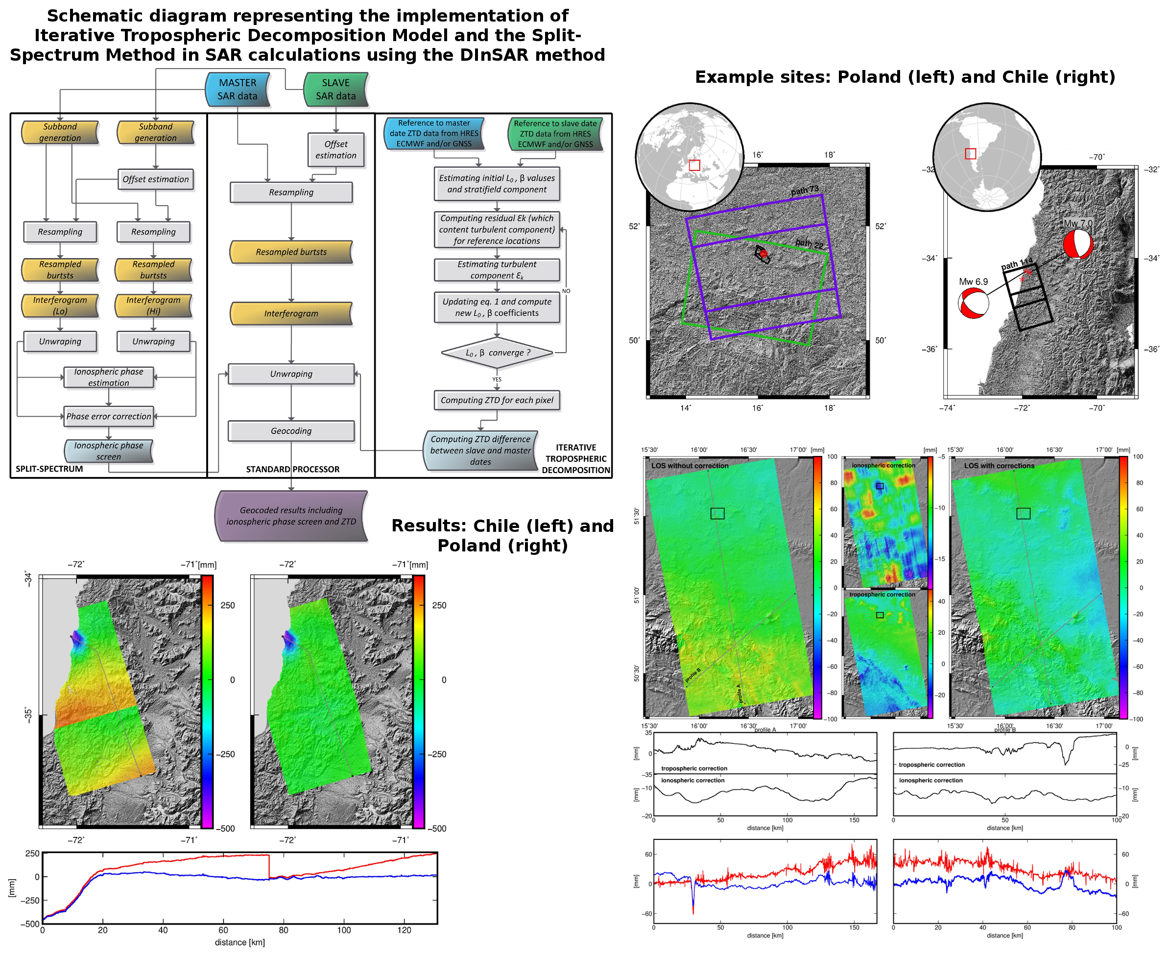
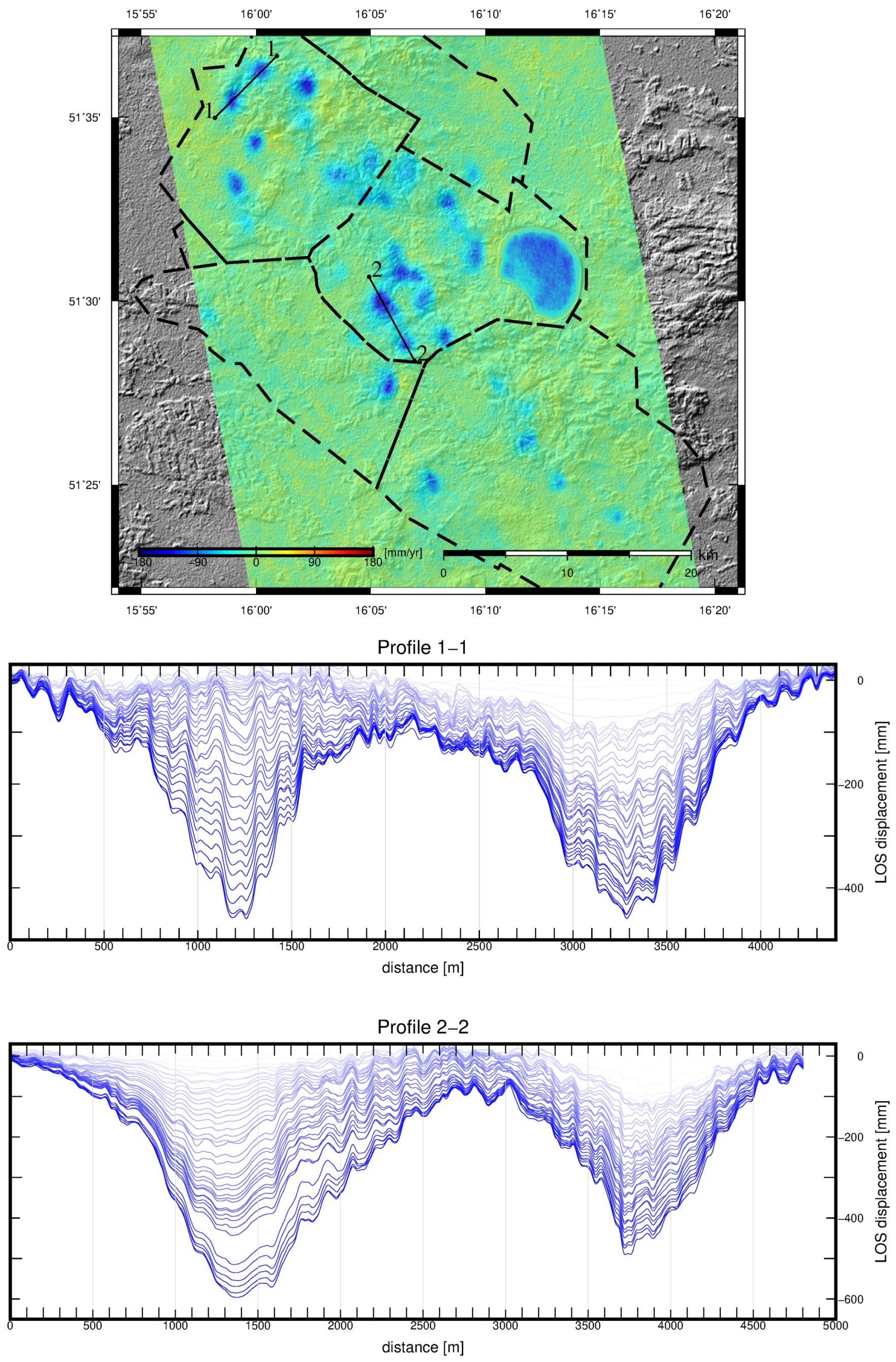
2.1. Tropospheric Delay Correction

Tropospheric influence was reduced by employing a GACOS model, which is based on the ITD model [12,13]. The ITD allows to establish zenith total delay ($ZTD$) for pixel k having coordinate vector x (3), based on known ZTD values in the reference points (HRES ECMWF and/or GNSS). The delay is iteratively calculated by decomposing the signal into stratigraphic and turbulent components based on Equation (3).

$$ZT{D}_k=S(h_k)+T(x_k)+{\epsilon }_k$$

(3)

where: S is the stratigraphic component of tropospheric delay correlated with height h, T is the turbulent component, and k is the unmodeled part of the signal.

The stratigraphic component is represented for any pixel by exponential Function (5), and values are interpolated using the inverse distance weighting (IDW) method.

$$S=L_o{e}^{-\beta h}$$

(4)

where $\beta$ is the exponential function coefficient, and $L_0$ is the stratigraphic delay component at sea level; the above coefficients are determined using the least-squares method on the basis of known $ZTD$ values. The turbulent component is interpolated on the basis of a modified IDW method:

$$T=\sum _{i=1}^n{w}_{ui}T(x_i),w_{ui}=d_{ui}^{-2}{/}_{{\sum }_{i=1}^n}{d}_{ui}^{-2}$$

(5)

where: u and i represent, respectively, the location for which T is calculated and a reference location of known T, $w_{ui}$ is the weight of delay T, an interpolation coefficient dependent on the horizontal distance between the interpolated point and reference point $d_{ui}$.

$$\left[\begin{array}{c}{T}_1\\ T_2\\ \dots \\ T_n\end{array}\right]=\left[\begin{array}{cccc}0& w_{12}& \dots & w_{1n}\\ w_{21}& 0& \dots & w_{2n}\\ \dots & \dots & 0& \dots \\ w_{n1}& \dots & w_{n,n-1}& 0\end{array}\right]\left[\begin{array}{c}{\epsilon }_1\\ {\epsilon }_2\\ \dots \\ {\epsilon }_n\end{array}\right]$$

(6)

In the first iteration of Equation (4), the turbulent component assumes a value of zero, and the delay it causes remains within the range of the unmodeled part of signal k. The turbulent component is calculated independently from the unmodeled part of the signal from Equation (7), with allowance for the weights of Equation (6).

The determined turbulent component is introduced into Equation (4), and coefficients $L_0$ and $\beta$ are calculated again. The iterative process is continued for as long as is necessary for coefficients $L_0$ and $\beta$ to converge to a certain value.

2.2. Ionospheric Delay Correction

The interferometric phase may be described with Equation (7), which includes a dispersive and a nondispersive component.

$$\Delta \varphi =\underset{non-dispersive}{\underbrace{{\displaystyle \frac{4\pi f_0}{c}}(\Delta r_{topo}+\Delta r_{defo}}}+\underset{dispersive}{\underbrace{\Delta r_{tropo})-{\displaystyle \frac{4\pi K}{c{f}_0}}\Delta TEC}}$$

(7)

where $f_o$ is the carrier frequency, $\Delta r_{topo}$, $\Delta r_{defo}$ and $\Delta r_{tropo}$ are, respectively, the topographic and deformation components, tropospheric path delay K is a constant equal to $40.28\frac{m^3}{s^2}$, and $\Delta TEC$ is difference $TEC$ between two acquisitions.

Unlike the troposphere, the ionosphere is a dispersive medium. This fact allows the ionospheric component to be isolated from the remaining part of the signal.

$$\begin{array}{c}\Delta {\varphi }_L=\Delta {\varphi }_{non-disp}{\displaystyle \frac{f_L}{f_0}}+\Delta {\varphi }_{iono}{\displaystyle \frac{f_0}{f_L}}\\ \Delta {\varphi }_H=\Delta {\varphi }_{non-disp}{\displaystyle \frac{f_H}{f_0}}+\Delta {\varphi }_{iono}{\displaystyle \frac{f_0}{f_H}}\end{array}$$

(8)

The ionospheric delay component was calculated using the split-spectrum method. The procedure consists of generating two subranges for a higher $f_L$ and a lower $f_H$ frequency, respectively. These serve to calculate two interferograms, $\Delta {\varphi }_L$ and $\Delta {\varphi }_H$, per Equation (8).

Transformation of Equation (8) for the interferograms for the two subranges produces equations that are sum of dispersion $\Delta {\varphi }_{iono}$ and nondispersion components $\Delta {\varphi }_{non-iono}$ Equation (9).

$$\begin{array}{c}\Delta {\widehat{\varphi }}_{iono}={\displaystyle \frac{f_L{f}_H}{f_0(f_H^2-f_L^2)}}(\Delta {\varphi }_L{f}_H-\Delta {\varphi }_H{f}_L)\\ \Delta {\widehat{\varphi }}_{non-disp}={\displaystyle \frac{f_0}{(f_H^2-f_L^2)}}(\Delta {\varphi }_H{f}_H-\Delta {\varphi }_L{f}_L)\end{array}$$

(9)

Figure 1 shows a schematic diagram representing the implementation of the Iterative Tropospheric Decomposition model and split-spectrum method for obtained data from the Sentinel satellites. Calculations of tropospheric and ionospheric delays are independent. Delays are allowed for after the interferometer baseline phase is unwrapped, and subsequently calculated into LOS displacements and geocoded.

3. Application Examples

The simultaneous allowance for ionospheric and tropospheric delays was used in DInSAR calculations for two areas (Figure 2). The first area is a region in southwestern Poland, where copper ore has been extracted using underground-mining methods since the 1970s. The second area is located in the western coast of Chile, which is one of the most seismically active regions on the planet.

Table 2. Scene-acquisition basic information.

Date and Time of Event (UTC) (Day/Month/Year)	Type	Strength [${\mathit{M}}_{\mathit{w}}$]	Event Location	Satellite	Master Date and Time (UTC) (Day/Month/Year)	Slave Date and Time (UTC) (Day/Month/Year)	Path
29/11/2016 8:09:39 P.M.	Induced tremor	4.2		Sentinel 1A	28/11/2016 4:43:20 P.M.	10/12/2016 4:43:20 P.M.	73
7/12/2017 5:42:50 P.M.	Induced tremor	4.5	Poland, the LGCB region	Sentinel 1A/1B	5/12/2017 4:43:33 P.M.	11/12/2017 4:42:51 P.M.
29/1/2019 12:53:45 P.M.	Induced tremor	4.1		Sentinel 1A/1B	26/1/2019 5:09:03 A.M.	1/2/2019 5:08:27 A.M.	22
11/3/2010 2:55:27 P.M.	Natural earthquake	7.0	Chile, Cardenal Caro province	ALOS 1	9/3/2010 4:03:29 A.M.	24/4/2010 4:03:06 A.M.	114
					9/3/2010 4:03:03 A.M.	24/4/2010 4:03:15 A.M.

includes basic information on the used SAR data. Calculations were performed in the GMT ver. 5.4.4 environment [42] and in GMTSAR [43]. In the GMTSAR environment, calculations using the DInSAR method were supplemented with an algorithm for calculating ionospheric correction based on the split-spectrum method [16], with filtering suggested by Fattahi [19]. Interferometric phase was unwrapped with the use of the Snaphu environment [40]. Wave-phase correction in relation to the ground surface was performed with Shuttle Radar Topography Mission (SRTM) version 1 [44]. The radar data from the Sentinel 1A/B satellites operated under the Copernicus program of the European Space Agency (ESA) and were retrieved from https://scihub.copernicus.eu/dhus/. The data from the ALOS-1 satellite were retrieved from the Alaska Satellite Facility (Dataset:© JAXA/METI ALOS PALSAR L1.0 2007. Accessed through ASF DAAC, 9 January 2019).

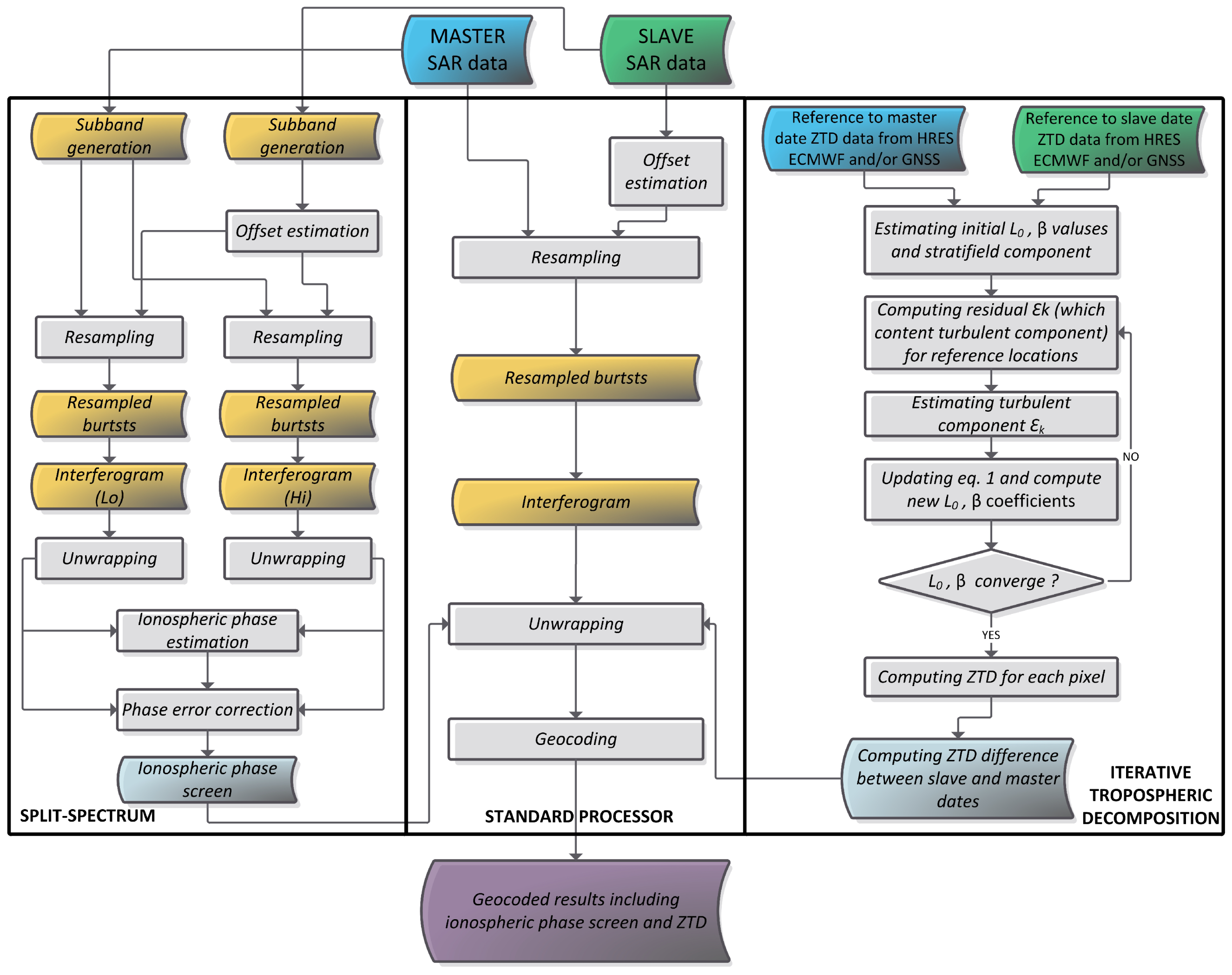
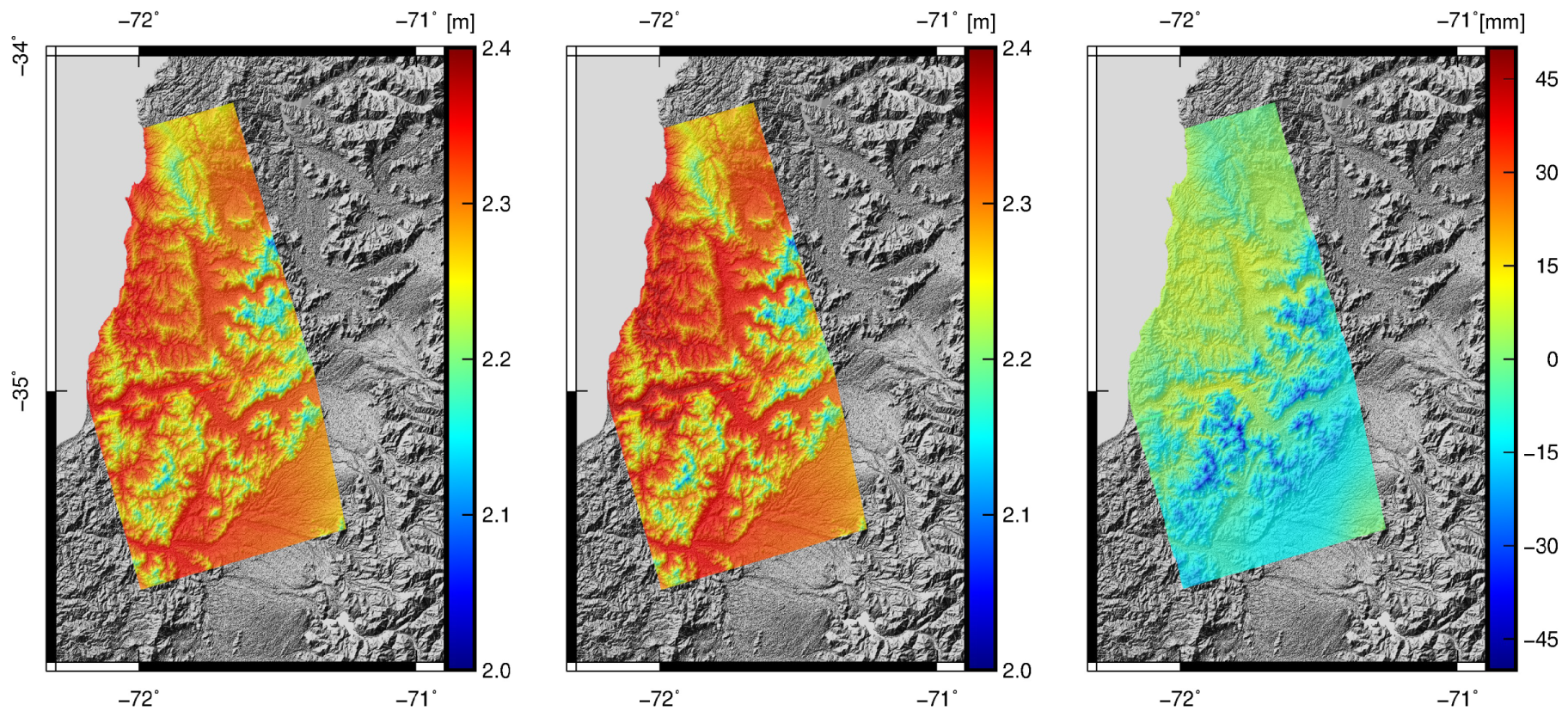
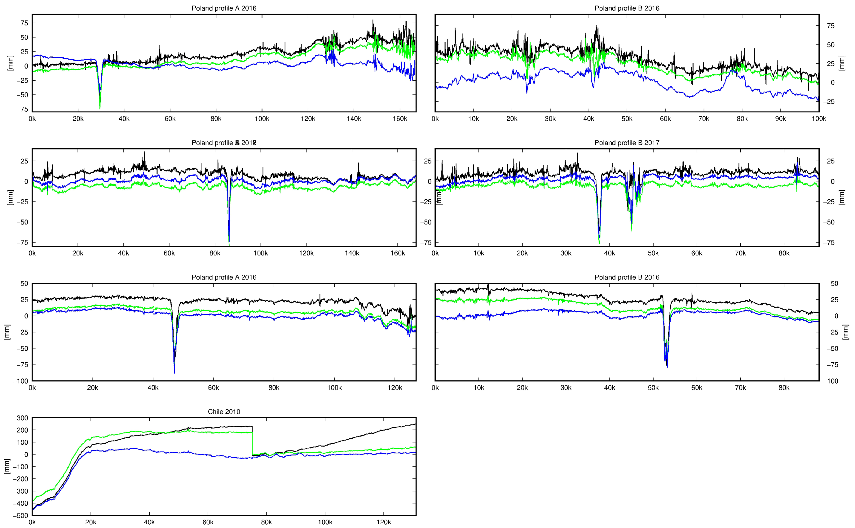
3.1. Legnica-Glogow Copper Belt Area

Induced seismic events occur as a result of human activity (e.g., mining operations, detonations of powerful explosives). As a result of such activity, rock mass may be disturbed. This, in turn, may lead to a tremor in which accumulated potential energy is released. Part of the released energy propagates in the form of elastic waves from the tremor center.

The exploitation of copper ore in the Legnica-Glogow Copper Belt (LGCB) area is performed at a depth of more than 1 km using the room-and-pillar method. Compared with average conditions in this part of Europe, this area shows high seismic activity. All of this activity is related to the processes of stress relief in intensively mined rock mass. Therefore, the observed tremors in the LGCB region are induced phenomena. Every year, the region suffers from several seismic events exceeding a magnitude of Mw 4.0. Some of these tremors result in recorded ground-surface subsidences [2,3], most of which are located in already existing subsidence troughs. Figure 3 shows the sum of subsidences (LOS) calculated for the period of 2014–2018. They illustrate how intensively underground extraction influences the ground surface. Calculations were performed with the SBAS time-series method [45]. Results clearly demonstrate the areas on the surface affected by underground-mining activity. Graphs show an increase in deformations resulting from underground copper-ore mining. As can be observed, most deformation increases are constant. This fact is due to the mining system adopted by the mining operations.

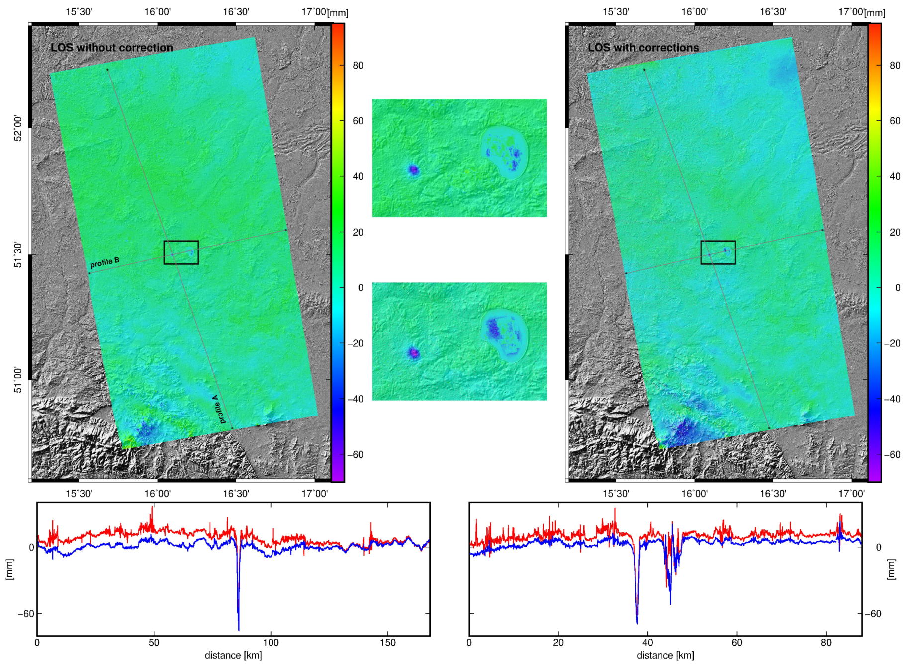
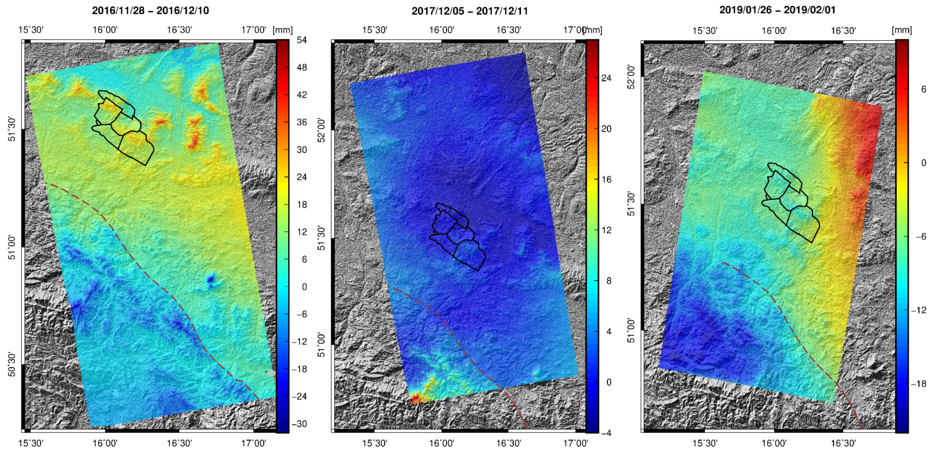
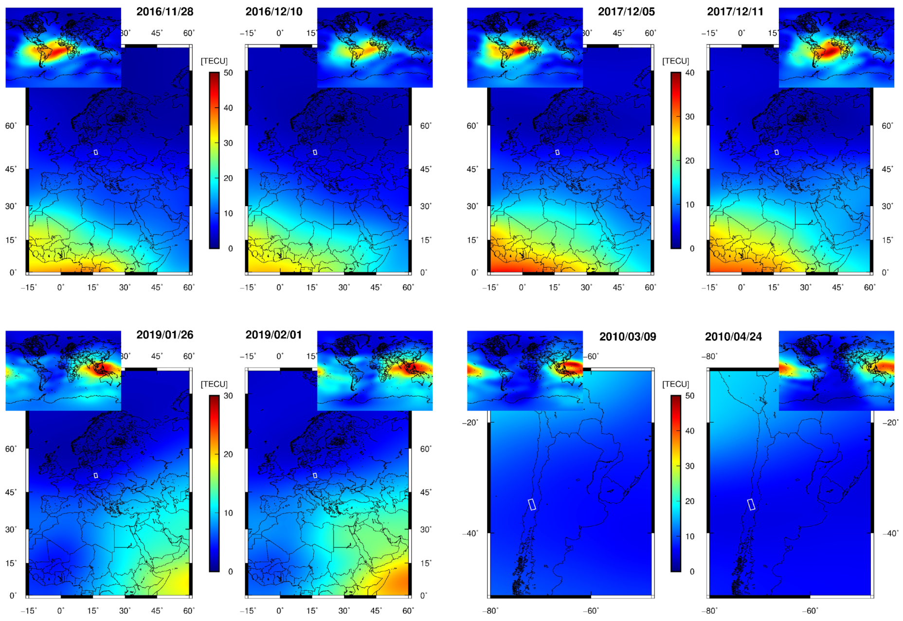
3.2. Induced Tremor on 29 November 2016

The first of the analyzed seismic events was the tremor on 29 November 2016. It was recorded in close vicinity to the Zelazny Most postflotation tailings pond. The reservoir stores postflotation waste produced as a results of copper-ore enrichment, and is the largest such engineered structure in Europe. The epicenter of the tremor was recorded at a distance of about 900 m from the western side of the reservoir’s embankments. Figure 4 shows the original interferogram, the estimated ionospheric phase screen, and the interferogram after ionospheric compensation.

Figure 5 shows the original unwrap phase, the delay difference between the images, and final unwrap phase, including tropospheric delay.

Figure 6 presents the calculated LOS displacements for the analyzed region without allowance for corrections, values, and spatial range of ionospheric and tropospheric corrections, as well as the final result. Displacement changes were plotted for two selected cross-sections. The first graph is approximately in accordance with the N–S direction. The graph is drawn across the created trough as a result of a mining tremor. The second graph follows the SW–NE direction. In the eastern part, the profile crosses the Sleza Massif, where the tropospheric correction assumes its maximum negative value of −31 mm.

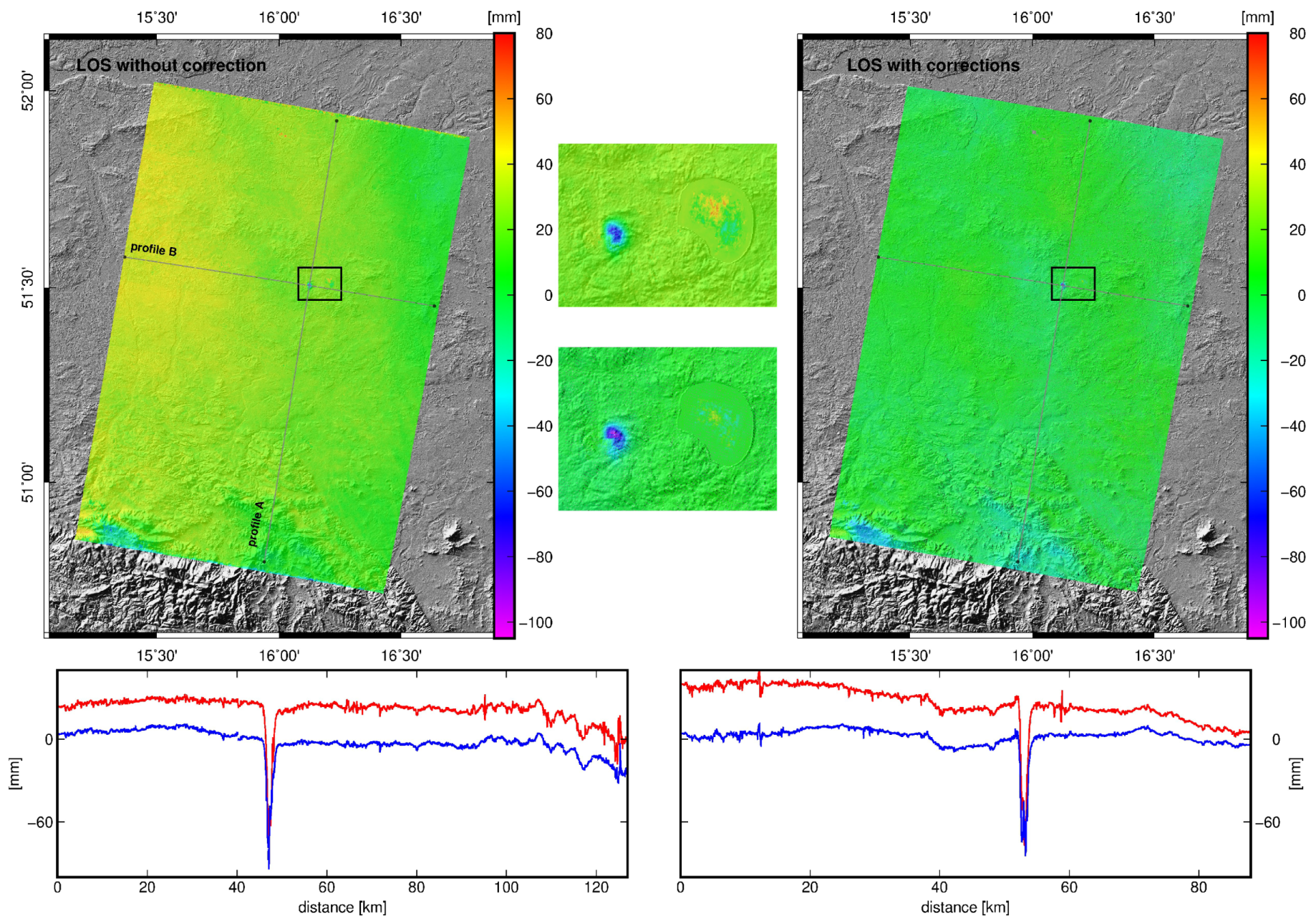
3.3. Induced Tremor on 7 December 2017

Of the three analyzed tremors that occurred in the LGCB region, the tremor on 7 December 2017 was the strongest. Its magnitude was about Mw 4.5. Data analysis from SBAS calculations indicates that the tremor resulted in ground subsidence at a maximum of −60 mm. As was previously the case, this subsidence also occurred in an already existing subsidence trough. Figure 7 shows the obtained results for this tremor.

3.4. Induced Tremor on 29 January 2019

The last tremor occurred on 29 January 2018. It had a magnitude of Mw 4.1. Our experience so far indicates that, in order to observe the results of induced mining tremors in the LGCB area, their magnitude should be at least Mw 4.0.

In the case of the LGCB area, analysis focused on three strong anthropogenic seismic events. For each event, DInSAR calculations served to identify ground-surface deformations. We present the resulting deformations for each tremor in Figure 6, Figure 7 and Figure 8. When comparing the range and location of the subsidence troughs with the results provided by the SBAS method (Figure 3), we concluded that each of the troughs was located in a deformation area related to underground mining activity. This fact is yet further proof that the discussed tremors have an anthropogenic character.

In accordance to the proposed calculation procedure (Figure 1), the ITD model was used to calculate the tropospheric delay difference for each SAR pair. The delay range for the analyzed LGCB area in successive periods was, respectively, −31/54 (2016), −4/27 (2017), and −22/10 (2019) mm. Figure 9 shows tropospheric correction values for individual periods. Within the scope of analysis for the whole area, minimum tropospheric correction values occurred in 2017. Only in the southwestern mountain region, did their value oscillate around 20 mm. In other regions, the correction showed values oscillating around zero (±3 mm). The greatest local gradients for the correction were observed in the period of the first analyzed tremor. In this case, there was a clearly visible border between the Sudeten Foreland and the actual Sudeten range. The observed values of the tropospheric refraction are highly correlated with the terrain topography (especially clearly visible in 2016). The influence of the Sudeten Massif is clear for all the three analyzed periods. From a geological perspective, responsibility is on the Sudetic Marginal Fault (Figure 9). The greatest changes of refraction values within the LGCB mining areas were also observed for 2016. They ranged from 5 to 30 mm. In the case of two events, the LGCB area showed a relatively constant value of tropospheric correction: from −3 to 3 mm for the 2017 event, and from −9 to −2 mm for the 2019 event. The surface results of the mining tremors had a local character. The spatial range of the calculated ground subsidences was 2.6 × 2.1 km (for the 2016 event) 1.2 × 1.3 km (2017), and 2.1 × 1.6 km (2019). Within the range of ground-surface deformations, the tropospheric correction in all analyzed periods had constant values, approximately 2 (2016), 1 (2017), and −7 mm (2019).

Analysis of the observed changes in the profiles concludes that allowing for corrections significantly improved the final results. In the case of the first 2016 event, Profile A showed a significant improvement. The output data showed high local variation, especially in mountain regions (southern part of the profile). The graph indicates clear growth from the north to the south. After applying the corrections, it was possible to observe two significant changes. First, local displacement variations were significantly reduced. Displacements in the profile were more gentle. Second, growth from the north to the south was eliminated. The observed tremor location did not change after applying corrections. The correction resulted in a slightly reduced maximum of the subsidence trough. Analysis of Profile B lead to similar conclusions. Only the region of the Sleza Massif (80 km in the profile) showed local anomaly, which was related to the local minimum observed in the tropospheric correction. By allowing for corrections in the two other examples, we were also able to significantly improve the final results. The 2017 results without corrections show much higher local-displacement variations that were reduced after applying the corrections. In this case, maximum values in the tremor-affected deformation area did not change. The results for the 2019 event were different. The observed output displacements in the profiles showed smaller variation than in the other cases. Within the limits of each of the sections a constant displacement of about 20 mm could be observed, which was corrected as a result of applying compensations. Deformations due to the 2017 and 2019 tremors had a similar range both before and after the corrections. As expected, the values of ionospheric refraction are relatively small. This is due to geographical location, SAR data-acquisition times, and the used C-band.

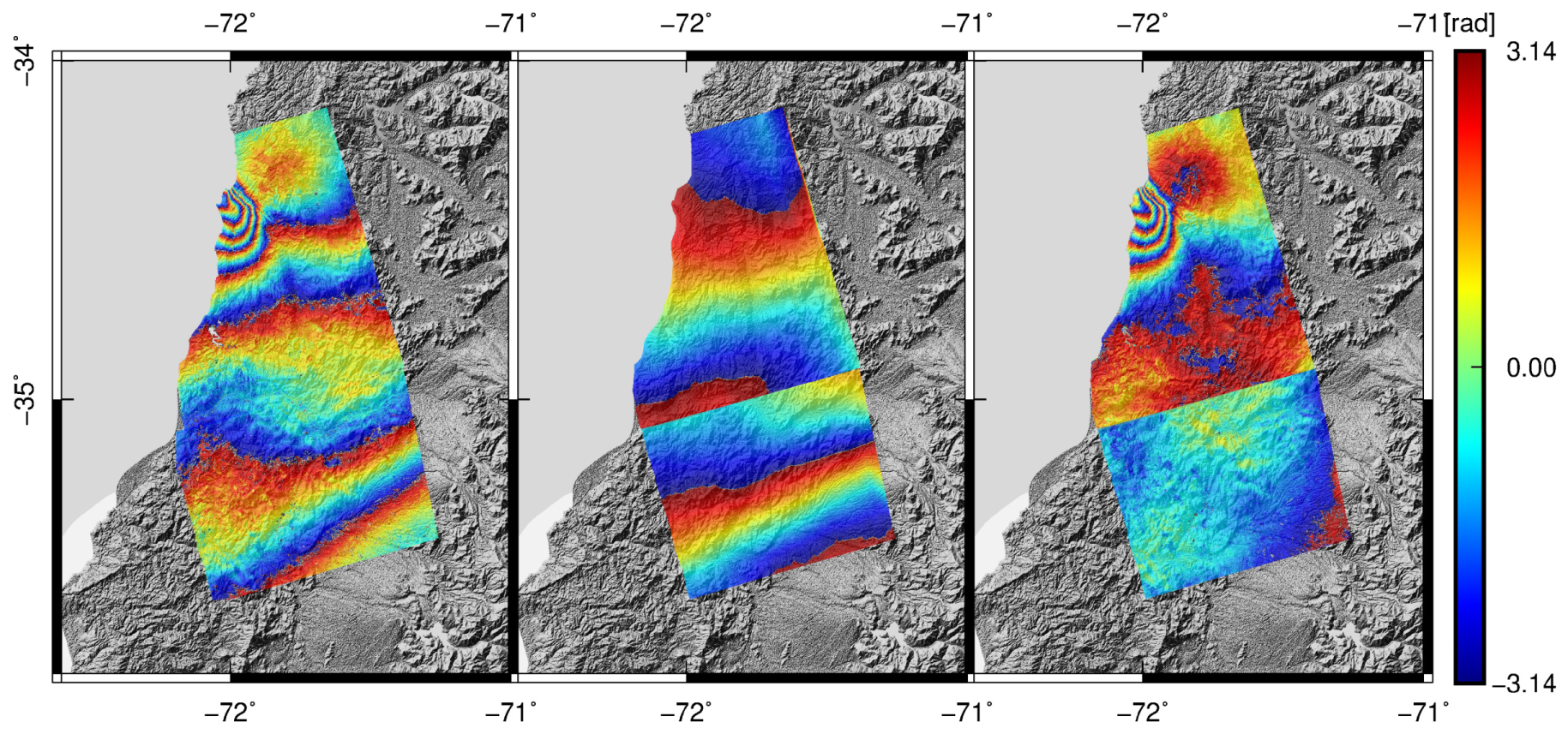
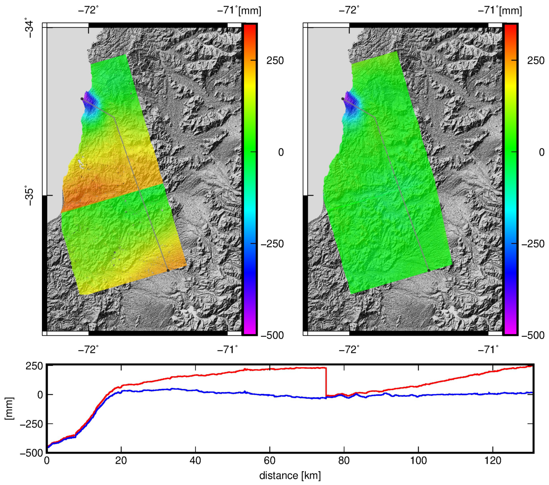
3.5. Chile—Natural Earthquake on 11 March 2010

The analyzed earthquake occurred at 14:55 (UTC), about fifteen kilometers northeast of Pichilemu, the capital of the Cardenal Caro province (O’Higgins Region, Libertador). It had a magnitude of Mw 7.0 and, within the next 40 min, it was followed by two additional events of Mw 6.0 and 6.9 magnitude, respectively. Like the whole coast of Chile, the region affected by the earthquakes is one of the most seismically active areas on the planet. It constitutes the western part of the Ring of Fire. The 2010 earthquake is the resulting thrust faulting generated at the gently sloping plate-boundary fault that conveys the Nazca plate eastward and downward beneath the South American plate [46]. Figure 10 shows the original interferogram, the ionospheric phase screen, and the interferogram with allowance for the influence of the ionosphere. The area affected by the earthquake is clearly visible (about 22 × 13 km). Figure 11 shows the spatial distribution of the tropospheric delay for master and slave data. The figure also shows delay differences between two images, which we used to reduce delay in subsequent calculations. The final result, a comparison of displacements before and after corrections, is presented in Figure 12.

The influence of the ionosphere on the interferogram phase is more evident in the case of the ALOS-1 satellite (Figure 10). Data from Sentinel 1 do not indicate such significant changes (Figure 4). At the same time, the tropospheric correction viewed as a delay difference between slave and master acquisitions was −49 mm (Figure 11). In the coastal regions, correction value was significantly smaller and oscillated around 7 mm. As was the case in the first Polish event, correlation of the value and terrain topography is clear. Coseismic deformations in the region were about 5 mm.

As a result of applying corrections, observed displacements on Path 114 for the period of 9 March 2010–24 April 2010 were significantly improved. No significant changes were observed in the region of coseismic deformations. The displacements in the profile, both before and after corrections, were almost identical until about 18 km. Only later did the original data show a growth trend. Maximum values reached 250 mm in each frame. There is, however, an important difference between the results for Chile and those for Poland. In the case of the data acquired for the Cardenal Caro province, no local displacement oscillations were observed to correspond to those from 2016 and 2019 (Figure 7 and Figure 8).

4. Discussion

As mentioned in the introduction, time and the spatial variability of atmospheric conditions have the most significant influence on the accuracy of performed measurements using InSAR methods. This is one of the reasons why problems related to allowing for these variables have become the object of so many research projects (Table 1). By allowing for corrections in the case of the LGCB mining areas, we were able to generally improve the displacement results. Each of the analyzed tremors resulted in a subsidence trough. Additionally, we demonstrated that the observed subsidences were located in already existing terrain-subsidence areas resulting from underground-mining activity. Our findings are based on a comparison of the obtained results (DInSAR) with time-series calculations (SBAS).

Displacements for the 2016 event are similar to the 2017 displacements. In both cases, the original data showed clear local displacement fluctuations that were limited as a result of further calculations. The results of the 2019 event are different, however. Local fluctuations are, in this case, not as high as in the previous cases. We believe that this fact is due to the less significant influence of the ionosphere. The 2016 and 2017 events were analyzed on the basis of SAR data obtained from Path 73. In the case of this path, acquisition time for the regions of southwestern Poland was approximately 16:43 (UTC) (Table 2). In the case of the 2019 event, we used SAR data obtained from Path 22. Acquisition time for this region was approximately 05:09 (UTC). Based on the provided data by monitoring ionosphere fluctuations, it may be assumed that, in the case of data from Path 73, the influence of the ionosphere would be greater. Using the obtained TEC data from the International GNSS Service (IGS), we prepared TEC maps for Poland and for Chile (Figure 13). Time resolution of the IGS data was 2 h, and spatial resolution was 2.5/5.0 degrees [47]. We selected optimal time intervals for each SAR acquisition.

Due to their time and spatial resolution, IGS data are only approximate. Nonetheless, we used them to conclude that the greatest values are related to Chile and are, respectively, 7.5 and 8.0 TECU. Meanwhile, in the case of Poland, TEC values for successive slave and master images are, respectively, 5.0/5.0 (2016), 4.0/4.5 (2017) and 2.5/3.0 (2019) TECU. In the analyzed regions, TEC maps do not provide sufficient information to clearly define the influence of ionospheric correction on the final displacement. For this reason, we prepared a comparison of displacements (Figure 13) in the profiles presented in Figure 6, Figure 7 and Figure 8, and Figure 12.

A comparison of LOS displacements in profiles without corrections, with ionospheric correction and with ionospheric and tropospheric corrections, confirms previous observations. The greatest noise was present in the 2016 and 2017 profiles (Poland). At the same time, the most limited fluctuations were observed in the analyzed region in Chile. It is worth noting that the calculated displacements (maximum values and ranges) for the event-affected areas did not change after applying corrections in any of the cases.

The comparison (Figure 14) indicates that ionospheric correction significantly reduces local variation. The result of its application is best illustrated in the comparison of displacements for the first analyzed period. Its least significant influence is observed in the case of the 2017 induced tremor and of the 2010 earthquake. The Polish examples demonstrate that the global (i.e., within the whole analyzed range—profile length) share of ionospheric correction was much lower as compared to tropospheric correction values. The results for Chile are different here.

Application of tropospheric correction improves displacement results to such a degree that they become de facto an “image” of output displacements (with limited local variations) transformed by a vertical vector. This fact is best seen in the case of the 2017 event and of the 2010 earthquake. The latter example may again be viewed as different from the other cases. Unlike in the case of Poland, analysis of the Chile earthquake is based on two frames from Path 114 (Table 2). The border between the images is clearly visible in the presented results. The situation is similar with the calculated ionospheric correction. Tropospheric correction based on the ITD model was calculated for a larger area.

5. Conclusions

This article presented the results of implementing atmospheric corrections in SAR data calculations with the use of the DInSAR method. We used the proposed calculation model (Figure 1) in four areas. The first three areas were related to underground-mining activity and showed induced anthropogenic tremors. The observed tremor strength in these areas in relation to natural earthquakes was not great. Nonetheless, as demonstrated in the article, tremors may result in ground-surface deformations. The other area is a region on the coast of Chile, which is part of the Ring of Fire. In this area, we analyzed a series of three earthquakes, the strongest of them with a magnitude of Mw 7.0. Based on the obtained data from ALOS-1, we calculated coseismic deformations, while simultaneously allowing for atmospheric corrections. This research enabled us to formulate the following conclusions:

Data from Sentinel 1A/B satellites allowed the detection of ground-surface deformations due to induced seismic events. This information is valuable, as the literature lacks descriptions of the potential of using synthetic aperture radar interferometry to detect the influence of induced seismic activity. The local character of the detected ground deformations (in the order of 2–3 km), and the possibility to precisely determine subsidence range, constitute important information.

We demonstrated that deformations related to mining-induced tremors are located in already existing terrain-subsidence areas. These areas are, in turn, the result of underground-mining activity. Our observations are based on a comparison between the results of DInSAR calculations and calculation results with the use of a time-series method (SBAS) that, in our case, relied on a large number of images (over 120).

Application of ionospheric and the tropospheric corrections significantly improved the final calculation results. One of the most important observations was that correction implementation did not produce modified maximum ground-surface deformation values in the regions affected by either induced tremors or natural earthquakes. Significant modifications were observed in areas where ground-surface deformations did not occur. Correction application eliminated many of the local displacement fluctuations and of their global shifts. Analysis of the influence of individual corrections led us to conclude that each correction affects the final results differently. Ionospheric correction significantly reduces local variations (fluctuations), while tropospheric correction is more responsible for the global (regarding the SAR data range) shift. The obtained results relate to two specific areas. Further research should be carried out in other areas to confirm the proposed solution.

Some issues still remain that require further research. Most importantly, the obtained values of ionospheric correction should be compared with (spatially) more precise TEC maps.

References

1. Albano, M.; Polcari, M.; Bignami, C.; Moro, M.; Saroli, M.; Stramondo, S. Did anthropogenic activities trigger the 3 April 2017 Mw 6.5 Botswana earthquake? Remote Sens. 2017, 9, 1028. [Google Scholar] [CrossRef]
2. Krawczyk, A.; Grzybek, R. An evaluation of processing InSAR Sentinel-1A/B data for correlation of mining subsidence with mining induced tremors in the Upper Silesian Coal Basin (Poland). E3S Web Conf. 2018, 26, 1–5. [Google Scholar] [CrossRef]
3. Malinowska, A.A.; Witkowski, W.T.; Guzy, A.; Hejmanowski, R. Mapping ground movements caused by mining-induced earthquakes applying satellite radar interferometry. Eng. Geol. 2018, 246, 402–411. [Google Scholar] [CrossRef]
4. Keranen, K.M.; Weingarten, M. Induced Seismicity. Ann. Rev. Earth Planet. Sci. 2018, 46, 149–174. [Google Scholar] [CrossRef]
5. Simons, M.; Fialko, Y.; Rivera, L. Earthquake as Inferred from InSAR and GPS Observations. Bull. Seismol. Soc. Am. 2002, 92, 1390–1402. [Google Scholar] [CrossRef]
6. Baer, G.; Magen, Y.; Nof, R.N.; Raz, E.; Lyakhovsky, V.; Shalev, E. InSAR Measurements and Viscoelastic Modeling of Sinkhole Precursory Subsidence: Implications for Sinkhole Formation, Early Warning, and Sediment Properties. J. Geophys. Res. Earth Surf. 2018, 123, 678–693. [Google Scholar] [CrossRef]
7. Xu, X.; Sandwell, D.T.; Tymofyeyeva, E.; González-Ortega, A.; Tong, X. Tectonic and Anthropogenic Deformation at the Cerro Prieto Geothermal Step-Over Revealed by Sentinel-1A InSAR. IEEE Trans. Geosci. Remote Sens. 2017, 55, 5284–5292. [Google Scholar] [CrossRef]
8. Tong, X.; Sandwell, D.T.; Smith-Konter, B. High-resolution interseismic velocity data along the San Andreas Fault from GPS and InSAR. J. Geophys. Res. Solid Earth 2013, 118, 369–389. [Google Scholar] [CrossRef] [Green Version]
9. Pagli, C.; Wang, H.; Wright, T.J.; Calais, E.; Lewi, E. Current plate boundary deformation of the Afar rift from a 3-D velocity field inversion of InSAR and GPS. J. Geophys. Res. Solid Earth 2014, 8562–8575. [Google Scholar] [CrossRef]
10. Tong, X.; Sandwell, D.T.; Schmidt, D.A. Surface Creep Rate and Moment Accumulation Rate Along the Aceh Segment of the Sumatran Fault from L-band ALOS-1/PALSAR-1 Observations. Geophys. Res. Lett. 2018, 45, 3404–3412. [Google Scholar] [CrossRef]
11. Bürgmann, R.; Rosen, P.A.; Fielding, E.J. Synthetic Aperture Radar Interferometry to Measure Earth’s Surface Topography and Its Deformation. Ann. Rev. Earth Planet. Sci. 2000, 28, 169–209. [Google Scholar] [CrossRef]
12. Yu, C.; Penna, N.T.; Li, Z. Generation of real-time mode high-resolution water vapor fields from GPS observations. J. Geophys. Res. 2017, 122, 2008–2025. [Google Scholar] [CrossRef] [Green Version]
13. Yu, C.; Li, Z.; Penna, N.T.; Crippa, P. Generic Atmospheric Correction Model for Interferometric Synthetic Aperture Radar Observations. J. Geophys. Res. Solid Earth 2018, 9202–9222. [Google Scholar] [CrossRef]
14. Brcic, R.; Parizzi, A.; Eineder, M.; Bamler, R.; Meyer, F. Estimation and compensation of ionospheric delay for SAR interferometry. Int. Geosci. Remote Sens. Symp. 2010, 2908–2911. [Google Scholar] [CrossRef]
15. Rosen, P.A.; Hensley, S.; Chen, C. Measurement and mitigation of the ionosphere in L-band Interferometric SAR data. IEEE Natl. Radar Conf. Proc. 2010, 1459–1463. [Google Scholar] [CrossRef]
16. Gomba, G.; Parizzi, A.; Zan, F.D.; Eineder, M.; Member, S.; Bamler, R. Toward Operational Compensation of Ionospheric Effects in SAR Interferograms: The Split-Spectrum Method. IEEE Trans. Geosci. Remote Sens. 2016, 54, 1446–1461. [Google Scholar] [CrossRef]
17. Böhm, J.; Schuh, H. (Eds.) Atmospheric Effects in Space Geodesy; Springer: Berlin/Heidelberg, Germany, 2013. [Google Scholar]
18. Shim, J.A.S. Analysis of Total Electron Content (TEC) Variations in the Low- and Middle-Latitude Ionosphere. Ph.D. Thesis, Utah State University, Logan, UT, USA, 2009. [Google Scholar]
19. Fattahi, H.; Simons, M.; Agram, P. InSAR Time-Series Estimation of the Ionospheric Phase Delay: An Extension of the Split Range-Spectrum Technique. IEEE Trans. Geosci. Remote Sens. 2017, 55, 5984–5996. [Google Scholar] [CrossRef]
20. Gomba, G.; Rodriguez Gonzalez, F.; De Zan, F. Ionospheric phase screen compensation for the Sentinel-1 TOPS and ALOS-2 ScanSAR modes. IEEE Trans. Geosci. Remote Sens. 2017, 55, 223–235. [Google Scholar] [CrossRef]
21. Rignot, E.J.M. Effect of Faraday rotation on L-band interferometric and polarimetric synthetic-aperture radar data. IEEE Trans. Geosci. Remote Sens. 2000, 38, 383–390. [Google Scholar] [CrossRef] [Green Version]
22. Wright, P.A.; Quegan, S.; Wheadon, N.S.; Hall, C.D. Faraday rotation effects on L-band spaceborne SAR data. IEEE Trans. Geosci. Remote Sens. 2003, 41, 2735–2744. [Google Scholar] [CrossRef]
23. Meyer, F.; Bamler, R.; Jakowski, N.; Fritz, T. The Potential of Low-Frequency SAR Systems for Mapping Ionospheric TEC Distributions. IEEE Geosci. Remote Sens. Lett. 2006, 3, 560–564. [Google Scholar] [CrossRef]
24. Jung, H.; Lee, D.; Lu, Z.; Won, J. Ionospheric Correction of SAR Interferograms by Multiple-Aperture Interferometry. IEEE Trans. Geosci. Remote Sens. 2013, 51, 3191–3199. [Google Scholar] [CrossRef]
25. Baby, H.B.; Golé, P.; Lavergnat, J. A model for the tropospheric excess path length of radio waves from surface meteorological measurements. Radio Sci. 1988, 23, 1023–1038. [Google Scholar] [CrossRef]
26. Ernest, K.; Smith, J.; Weintraub, S. The Constants in the Equation for Atmospheric Refractive Index at Radio Frequencies. Proc. IRE 1953, 50, 1035–1037. [Google Scholar] [CrossRef]
27. Hanssen, R.F. Radar Interferometry: Data Interpretation and Error Analysis; Kluwer Academic: Dordrecht, The Netherlands, 2001. [Google Scholar]
28. Wicks, C.W.; Dzurisin, D.; Ingebritsen, S.; Thatcher, W.; Lu, Z.; Iverson, J. Magmatic activity beneath the quiescent Three Sisters volcanic center, central Oregon Cascade Range, USA. Geophys. Res. Lett. 2002, 29, 24–26. [Google Scholar] [CrossRef]
29. Lin, Y.N.; Simons, M.; Hetland, E.A.; Muse, P.; DiCaprio, C. A multiscale approach to estimating topographically correlated propagation delays in radar interferograms. Geochem. Geophys. Geosyst. 2010, 11. [Google Scholar] [CrossRef] [Green Version]
30. Bekaert, D.P.S.; Walters, R.J.; Wright, T.J.; Hooper, A.J.; Parker, D.J. Statistical comparison of InSAR tropospheric correction techniques. Remote Sens. Environ. 2015, 170, 40–47. [Google Scholar] [CrossRef] [Green Version]
31. Bekaert, D.P.S.; Hooper, A.; Wright, T.J. A spatially variable power law tropospheric correction technique for InSAR data. J. Geophys. Res. Solid Earth 2015, 120, 1345–1356. [Google Scholar] [CrossRef] [Green Version]
32. Tymofyeyeva, E.; Fialko, Y. Mitigation of atmospheric phase delays in InSAR data, with application to the eastern California shear zone. J. Geophys. Res. Solid Earth 2015, 120, 5952–5963. [Google Scholar] [CrossRef] [Green Version]
33. Doin, M.P.; Lasserre, C.; Peltzer, G.; Cavalié, O.; Doubre, C. Corrections of stratified tropospheric delays in SAR interferometry: Validation with global atmospheric models. J. Appl. Geophys. 2009, 69, 35–50. [Google Scholar] [CrossRef]
34. Löfgren, J.S.; Björndahl, F.; Moore, A.W.; Webb, F.H.; Fielding, E.J.; Fishbein, E.F. Tropospheric correction for InSAR using interpolated ECMWF data and GPS Zenith Total Delay from the Southern California Integrated GPS Network. In Proceedings of the 2010 IEEE International Geoscience and Remote Sensing Symposium, Honolulu, HI, USA, 25–30 July 2010; pp. 4503–4506. [Google Scholar] [CrossRef]
35. Jolivet, R.; Grandin, R.; Lasserre, C.; Doin, M.P.; Peltzer, G. Systematic InSAR tropospheric phase delay corrections from global meteorological reanalysis data. Geophys. Res. Lett. 2011, 38. [Google Scholar] [CrossRef] [Green Version]
36. Gong, W.; Meyer, F.; Webley, P.W.; Morton, D.; Liu, S. Performance analysis of atmospheric correction in InSAR data based on the Weather Research and Forecasting Model (WRF). In Proceedings of the 2010 IEEE International Geoscience and Remote Sensing Symposium, Honolulu, HI, USA, 25–30 July 2010; pp. 2900–2903. [Google Scholar] [CrossRef]
37. Li, Z.; Muller, J.P.; Cross, P.; Albert, P.; Hewison, T.; Watson, R.; Fisher, J.; Bennartz, R. Validation of MERIS Near IR Water Vapour Retrievals Using MWR and GPS Measurements. In Proceedings of the MERIS User Workshop, Frascati, Italy, 10–13 November 2003. [Google Scholar]
38. Li, Z.; Muller, J.P.; Cross, P.; Albert, P.; Fischer, J.; Bennartz, R. Assessment of the potential of MERIS near-infrared water vapour products to correct ASAR interferometric measurements. Int. J. Remote Sens. 2006, 27, 349–365. [Google Scholar] [CrossRef]
39. Li, Z.; Fielding, E.J.; Cross, P.; Preusker, R. Advanced InSAR atmospheric correction: MERIS/MODIS combination and stacked water vapour models. Int. J. Remote Sens. 2009, 30, 3343–3363. [Google Scholar] [CrossRef] [Green Version]
40. Cheng, S.; Perissin, D.; Lin, H.; Chen, F. Atmospheric delay analysis from GPS meteorology and InSAR APS. J. Atmos. Sol. Terr. Phys. 2012, 86, 71–82. [Google Scholar] [CrossRef]
41. Zhu, W.; Ding, X.L.; Jung, H.S.; Zhang, Q.; Zhang, B.C.; Qu, W. Investigation of ionospheric effects on SAR Interferometry (InSAR): A case study of Hong Kong. Adv. Space Res. 2016, 58, 564–576. [Google Scholar] [CrossRef]
42. Wessel, P.; Smith, W.H.F.; Scharroo, R.; Luis, J.; Wobbe, F. Generic Mapping Tools: Improved Version Released. Eos Trans. Am. Geophys. Union 2013, 94, 409–410. [Google Scholar] [CrossRef] [Green Version]
43. Sandwell, D.; Mellors, R.; Tong, X.; Wei, M.; Wessel, P. Open Radar Interferometry Software for Mapping Surface Deformation. Eos Trans. Am. Geophys. Union 2011, 92, 234. [Google Scholar] [CrossRef]
44. Farr, T.; Rosen, P.A.; Caro, E.; Crippen, R.; Duren, R.; Hensley, S.; Kobrick, M.; Paller, M.; Rodriguez, E.; Roth, L.; et al. The shuttle radar topography mission. Rev. Geophys. 2007, 45, 1–33. [Google Scholar] [CrossRef]
45. Berardino, P.; Fornaro, G.; Lanari, R.; Sansosti, E. A new algorithm for surface deformation monitoring based on small baseline differential SAR interferograms. IEEE Trans. Geosci. Remote Sens. 2002, 40, 2375–2383. [Google Scholar] [CrossRef]
46. Hayes, G.P.; Meyers, E.K.; Dewey, J.W.; Briggs, R.W.; Earle, P.S.; Benz, H.M.; Smoczyk, G.M.; Flamme, H.E.; Barnhart, W.D.; Gold, R.D.; et al. USGS Open-File Report 2016–1192. Tectonic Summaries of Magnitude 7 and Greater Earthquakes from 2000 to 2015. Tech. Rep. 2016. [Google Scholar] [CrossRef]
47. Hernández-Pajares, M.; Juan, J.M.; Sanz, J.; Orus, R.; Garcia-Rigo, A.; Feltens, J.; Komjathy, A.; Schaer, S.C.; Krankowski, A. The IGS VTEC maps: A reliable source of ionospheric information since 1998. J. Geod. 2009, 83, 263–275. [Google Scholar] [CrossRef]
Figure 1. Implementation of Iterative Tropospheric Decomposition model and split-spectrum method in SAR calculations using the differential InSAR (DInSAR) method (Sentinel 1).
Remotesensing 11 00621 g001
Figure 2. Ground coverage of Sentinel 1A/B acquisitions for (left) the Legnica-Glogow Copper Belt (LGCB) area and (right) the ALOS-1 acquisitions for the Chile example site.
Remotesensing 11 00621 g002
Figure 3. Sum of line-of-sight (LOS) displacements for LGCB mining areas, determined on the basis of data from Sentinel 1A/1B satellites, collected for the period of November 2014–May 2018 (top). Calculation was based on 122 SAR images from Path 73 using the SBAS method (total number of pairs, 436). Black dashed line indicates mining-area borders. (Bottom) increments of ground subsidences for two selected cross-sections.
Remotesensing 11 00621 g003
Figure 4. (left) Original Sentinel 1 interferogram from the LGCB area, containing the 2016 tremor (area marked with black polygon), (middle) estimated ionospheric phase screen, and (right) interferogram after ionospheric compensation.
Remotesensing 11 00621 g004
Figure 5. (left) Spatial range of original unwrap phase, (middle) delay difference between slave and master images, and (right) final result, unwrap phase including tropospheric delay.
Remotesensing 11 00621 g005
Figure 6. Results for the 2016 tremor. (left) LOS displacements calculated with the use of the DInSAR method (Sentinel 1, TOPS) for period of 28 November 2016–10 December 2016. Calculated values: (middle-top) ionospheric component, (middle-bottom) tropospheric component, and LOS displacements allowing for the above components. Graphs: Calculated values: ionospheric component and tropospheric component for each of the cross-sections (top). Comparison of results without allowance for corrections (red line) and with allowance (blue line) for ionospheric component and tropospheric component (bottom).
Remotesensing 11 00621 g006
Figure 7. Results obtained for the 2017 tremor, LOS displacements calculated with DInSAR (Sentinel 1, TOPS) for (left) the period of 12 May 2017–11 December 2017; (right) LOS displacements with allowance for the influence of the ionosphere and the troposphere. Red line indicates displacements without allowance for corrections, and blue line with allowance for corrections.
Remotesensing 11 00621 g007
Figure 8. Obtained results for the 2019 tremor, LOS displacements calculated with DInSAR (Sentinel 1, TOPS) for (left) the period of 26 January 2019–2 February 2019; (right) LOS displacements with allowance for the influence of the ionosphere and the troposphere. Red line indicates displacements without allowance for corrections, and blue line with allowance for corrections.
Remotesensing 11 00621 g008
Figure 9. Iterative Tropospheric Decomposition (ITD)-based calculations of tropospheric delay differences for successive calculation periods; dashed brown line indicates the Sudetic Marginal Fault.
Remotesensing 11 00621 g009
Figure 10. (left) Original ALOS-1 interferogram from the Cardenal Caro area containing the 2010 earthquake, (middle) estimated ionospheric phase screen, and (right) interferogram after ionospheric compensation.
Remotesensing 11 00621 g010
Figure 11. Spatial range of tropospheric delay for the following images: (left) slave (middle) master and (right) delay difference.
Remotesensing 11 00621 g011
Figure 12. Displacements calculated with the use of DInSAR method for two frames from Path 114 (left) without corrections and (right) with corrections; comparison of displacements before and after corrections in a selected profile (bottom).
Remotesensing 11 00621 g012
Figure 13. Total Electron Content (TEC) International GNSS Service (IGS) maps for successive SAR images; white polygons represent analyzed areas.
Remotesensing 11 00621 g013
Figure 14. Comparison of observed displacement fluctuations in the profiles. Black line denotes the original data; green line, results including ionospheric correction; blue line, results including both ionospheric and tropospheric corrections.
Remotesensing 11 00621 g014