A Recursive Update Model for Estimating High-Resolution LAI Based on the NARX Neural Network and MODIS Times Series


1
State Key Laboratory of Remote Sensing Science, Jointly Sponsored by Beijing Normal University and Institute of Remote Sensing and Digital Earth of Chinese Academy of Sciences, Beijing 100875, China
2
Beijing Engineering Research Center for Global Land Remote Sensing Products, Institute of Remote Sensing Science and Engineering, Faculty of Geographical Science, Beijing Normal University, Beijing 100875, China
3
College of Information and Management Science, Henan Agricultural University, Zhengzhou 450002, China
4
PowerChina Kunming Engineering Corporation Limited, Kunming 650051, China
*
Author to whom correspondence should be addressed.
Remote Sens. 2019, 11(3), 219; https://doi.org/10.3390/rs11030219
Submission received: 2 January 2019
/
Revised: 19 January 2019
/
Accepted: 21 January 2019
/
Published: 22 January 2019
(This article belongs to the Special Issue Leaf Area Index (LAI) Retrieval using Remote Sensing)
Abstract
:Leaf area index (LAI) remote sensing data products with a high resolution (HR) and long time series are in demand in a wide variety of applications. Compared with long time series LAI products with 1 km resolution, LAI products with high spatial resolution are difficult to acquire because of the lack of remote sensing observations in long-term sequences and the lack of estimation methods applicable to highly variable land-cover types. To address these problems, we proposed a recursive update model to estimate 30 m resolution LAI based on the updated Nonlinear Auto-Regressive with Exogenous Inputs (NARX) neural network and MODIS time series. First, we used a variety of HR satellite remote sensing observations to produce HR datasets for recent years. Historical low spatial resolution MODIS products were employed as background information and used to calculate the initial parameters of the NARX neural network for each pixel. Subsequently, one year’s reflectance from the HR dataset was used as the new observation that was input into the NARX model to estimate the HR LAI of that year, and the background and HR data were then used for remodeling to update the NARX model parameters. This procedure was recursively repeated year by year until both MODIS background data and all HR data were involved in the modeling. Finally, we obtained an LAI time series with 30 m resolution. In the cropland study area in Hebei Province, China, the results were compared with LAI measurements from ground sites in 2013 and 2014. A high degree of similarity existed between the results for the two study years ( and ). The HR LAI estimates showed favorable spatiotemporal continuity and were in good agreement with the multisample ground survey LAI measurements. The results indicated that for data with a rapid revisit cycle and high spatial resolution, the recursive update model based on the NARX neural network has excellent LAI estimation performance and fairly strong fault-tolerance capability.
1. Introduction
The leaf area index (LAI) is defined as the one-sided green leaf area per unit of horizontal ground area [1]. LAI is a critical input parameter for models related to ecological and environmental monitoring, crop modeling, and climate change [2]. The precise estimation of LAI is critical for its subsequent application. At present, various fields have widely used long-term global LAI products, such as Moderate Resolution Imaging Spectroradiometer (MODIS), Satellite Pour l’Observation de la Terre (SPOT/VEGETATION) and Advanced Very High Resolution Radiometer (AVHRR). However, land surfaces tend to be highly heterogeneous at coarse resolutions, and existing remote sensing LAI products fail to satisfy the need for regional research. In response to this demand, many studies have been conducted to provide long time series LAI data with high temporal and spatial resolutions [3].
Due to technological and economic restrictions, sensors with a short revisit cycle usually have a coarse spatial resolution; however, sensors with high spatial resolutions are associated with a longer time interval between acquisitions of data in the same region. The revisit cycle of Landsat Thematic Mapper (TM) data (30 m spatial resolution) is 16 days in most cases. If the area is prone to cloud or haze cover, there may be only one available data point in a month or two. Therefore, LAI products with long time series have in the past been characterized by low or medium resolutions (no better than 500 m). However, in recent years, with the continuous progress of science and technology, sensors of various types have been developed. Many satellites with high spatial resolutions and revisit cycles of less than 3 days have been launched, such as the small environment and disaster monitoring and forecasting satellite constellation HJ-1A/B, FORMOSAT-2, the WorldView satellites and Sentinel-2 [3,4,5,6].
The common algorithms used to estimate LAI based on remote sensing data are empirical regressions, nonparametric regressions, radiation transfer methods and hybrid methods [6,7]. In detail, the empirical regression approach normally uses remotely sensed imagery and terrestrial survey data acquired simultaneously to carry out multilinear regression modeling [8] or statistical models [9] to estimate LAI; most of these methods use various vegetation indices [10,11,12,13] as input parameters. Because these methods are subject to the availability of terrestrial survey data and to regional limitations, they are very difficult to generalize and use. LAI inversion using a radiative transfer model [14,15,16,17] is an extremely effective method with superior generality. However, due to the complexity of the radiative transfer model and the relatively finite nature of remote sensing observational data, considerable prior data should be included when using these models. Moreover, the input parameters have difficulty accurately describing the spatial and temporal variation characteristics of vegetation; in most cases, this difficulty leads to an ill-posed inversion [18,19]. The hybrid method combines elements of statistics and physically based methods [19,20,21]. This method has the advantages of high speed and flexibility and can produce uncertainty estimates. However, these methods may be difficult to use in practical applications.
Nonparametric regression methods estimate LAI without a priori assumptions [22] and are optimized with a training process using reference data. In contrast to empirical regression methods, nonexplicit choices need to be made regarding the spectral band relationships, transformation or fitting function. Neural networks belong to nonparametric methods [23]. An artificial neural network can not only process nonlinear, nonnormal, and collinear data that cannot be dealt with in a statistical model [24], but also has been extensively used in remote sensing data classification [25,26], biomass extraction [27,28], and LAI estimation [29,30,31], among other applications.
Currently, most high spatial resolution LAI estimation methods mainly use data fusion or neural network methods. Several data fusion methods have been proposed to combine high spatial resolution and high temporal resolution data to generate synthetic imagery with a high spatiotemporal resolution. For instance, the Spatial and Temporal Adaptive Reflectance Fusion Model (STARFM) [32] estimates high-resolution (HR) pixel values by combining information from all input images by weight functions. STARFM assumes that the change in reflectance is consistent and comparable in coarse and high resolutions, and the transfer function is empirical, so uncertainty is easily introduced during the transfer process.
The Nonlinear Auto-Regressive with Exogenous Inputs (NARX) model is a recurrent nonlinear dynamic neural network with a global feedback. In this model, autofeedback effects occur constantly during estimation, and this network has been widely used in timing sequence modeling. NARX has a rapid training and convergence speed and strong representativeness and is characterized by favorable dynamics and resistance to interference. The NARX is well suited for modeling the complicated nonlinear systems because of its long term-dependencies and its computational power [33,34]. It is demonstrated promising performance in research for time series modelling. By comparing validation period results, NARX showed a significant superiority over static neural networks [35]. For example, this method has been used for change detection in snow caps [36] and LAI time series estimation [37] based on MODIS data.
In this paper, a recursive update model using neural networks with a long time series auto-feedback function [38,39] was used to generate HR LAI time series. The new method has the following strengths: (1) it uses historical low spatial resolution MODIS nadir BRDF-adjusted reflectance (NBAR) and LAI time series as background information to estimate HR LAI; (2) it needs fewer predefined parameters; and (3) the estimation results have the advantage of a high temporal resolution (8 days) and a high spatial resolution (30 m). A recurrent update model was developed in this study and tested in eight pilot sites using HR images.
2. Methods
In a given area, if the crop type does not change, the phenological curve of different years has a strong similarity in time series. On this basis, we use a large amount of accumulated coarse-resolution remote sensing data to support high spatial resolution LAI estimation. First, a phenological change model of vegetation was trained using coarse spatial resolution remote sensing data. Then, in the phenological change model, the HR data were used as inputs to estimate the HR LAI. Finally, the coarse spatial resolution and high spatial resolution data were used to form the new time series training data; the phenological change modeling was performed again, and the model parameters were updated by taking advantage of the HR data. During the LAI estimation process, the phenological change model was refitted every time HR data were added to the training data. In this process, the node coefficients of the model were continually corrected to the estimation of high spatial resolution data, and finally, the goal of estimating high spatial resolution LAI was achieved.
2.1. Recursive Update Model
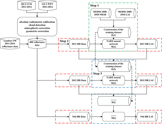
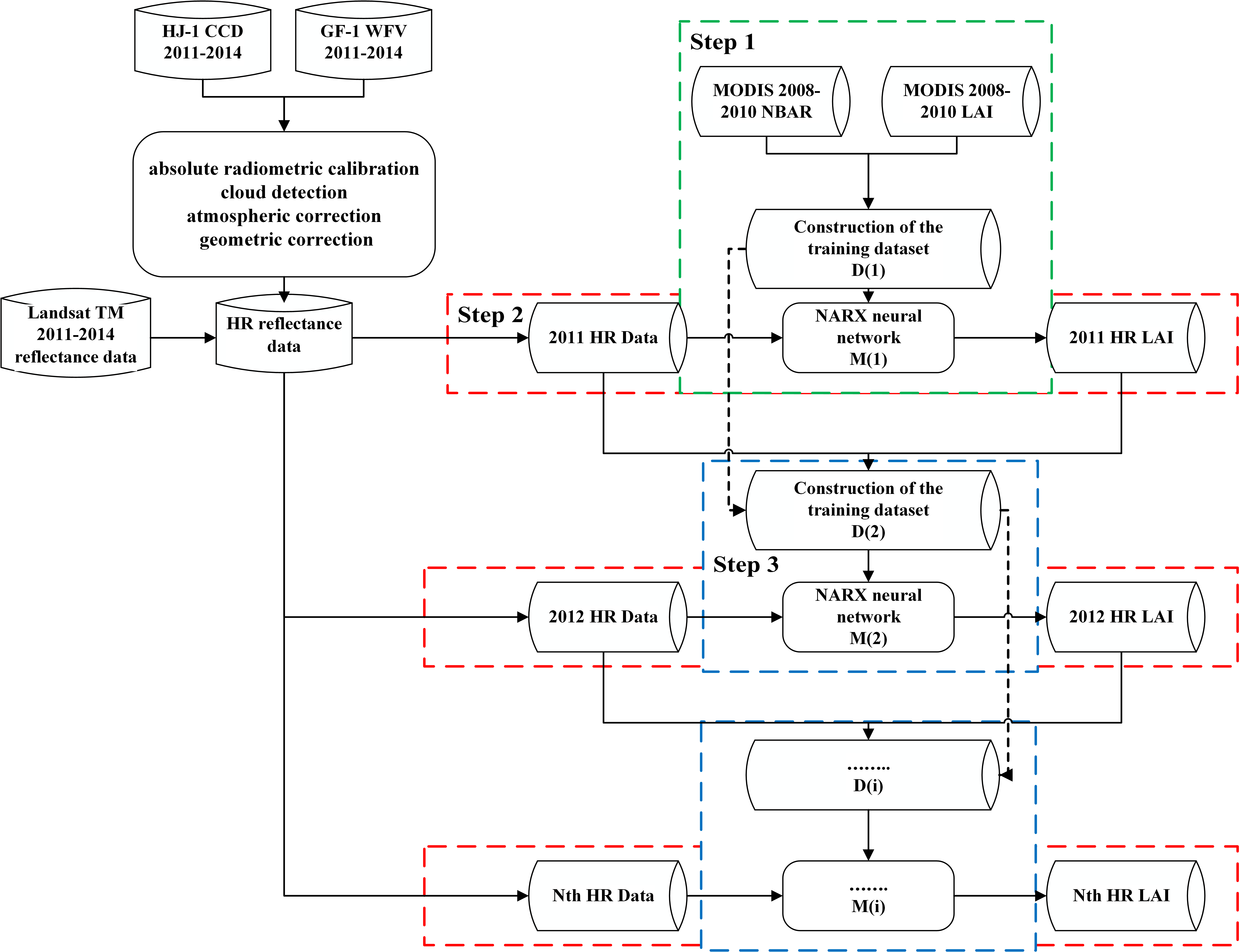
The algorithm proceeds through several stages shown in Figure 1, processing the images from one one-year time series at a time. The neural network is trained with coarse-resolution data, and a set of weights is obtained. To renew the weights, high spatial resolution LAI and coarse resolution data are simultaneously provided to the neural network, and the neural network is retrained with the new training set in each iteration. The recursive update process of the neural network is as follows:
Step 1: Create the NARX network for background information.
We use the MODIS NBAR and LAI time series of 2008–2010 (i.e., D(1) in Figure 1) as input for the neural network and to train the NARX neural network to estimate the LAI for each pixel. The neural network is trained on a reflectance database comprising radiative transfer model simulations. The relationship between the MODIS LAI and the reflectance time series is modeled (i.e., M(1) in Figure 1) and represented by the parameters of the neural network, which are taken as the time series background for further processing.
Step 2: HR LAI estimation
The HR time series surface reflectance in 2011 is used as input for the neural network (M(1)) to estimate HR LAI. Note that in this step, each HR pixel is taken as a subpixel of the related MODIS pixel. The background information of each MODIS pixel can be used as a priori knowledge of approximately 272 (500*500/30*30) HR pixels. In this step, although the retrieved HR LAI has a 30 m spatial resolution, it also contains substantial MODIS pixel information.
Step 3: Retraining of NARX networks.
High spatial resolution information is added to the training data, and the neural network is retrained using the same structure. In this step, the MODIS reflectance data of 2008-2010 and the HR reflectance data of 2011 are set as new inputs for the neural network, and the MODIS LAI of 2008–2010 and HR LAI of 2011 are set as the corresponding outputs to retrain the NARX neural network for each HR pixel. The new training dataset is called D(2). After creating a new training set, the neural network is retrained with D(2). The new set of NARX network weights is found (M(2)). This process changes the initial weights and biases of the network and may produce an improved network after retraining. Through updating of the neural network, the new coefficients contain information from both MODIS and the 30 m resolution datasets. Consequently, using the MODIS (500 m) and HR (30 m) data as the background, the LAI time series with HR pixels (30 m) is estimated.
Step 4: Recursive model construction.
Steps 2 and 3 are repeated for a number of iterations until all HR datasets are involved in the training. The effect of HR data on the LAI results gradually increases during the estimation process. In these cases, the recursive procedures provide model improvement.
By conducting recursive training, the proportion of HR information in the training data was increased, and the result can be considered HR LAI data. With the gradual increase in HR spatial detail, the retrieved results achieved the full complement of HR pixels. Using the proposed method, the neural network feedback is continually updated. As the HR images in the training data increase, a more accurate estimate of the 30 m resolution LAI can be obtained.
2.2. Application of the NARX Network
When using historical coarse spatial resolution data as a priori knowledge for the estimation of high spatial resolution LAI, we chose to use the NARX neural network to train time series data to extract the phenological characteristics. The NARX network is a nonlinear autoregressive network with exogenous inputs [39]. It is not only applicable to modeling and predicting nonlinear systems and time series, but is also able to achieve favorable outcomes for LAI estimation [37]. The general form of the NARX network can be expressed as follows:
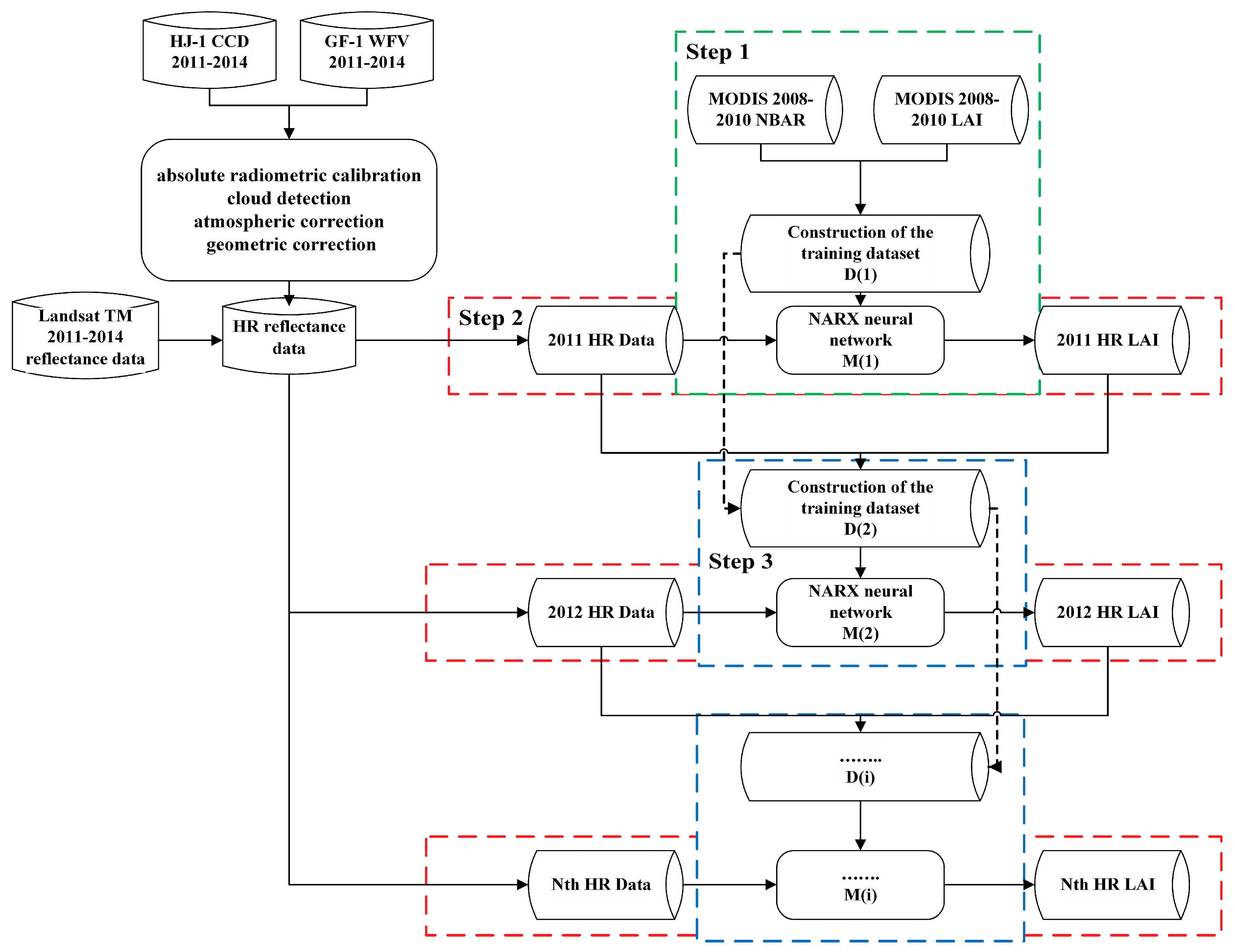
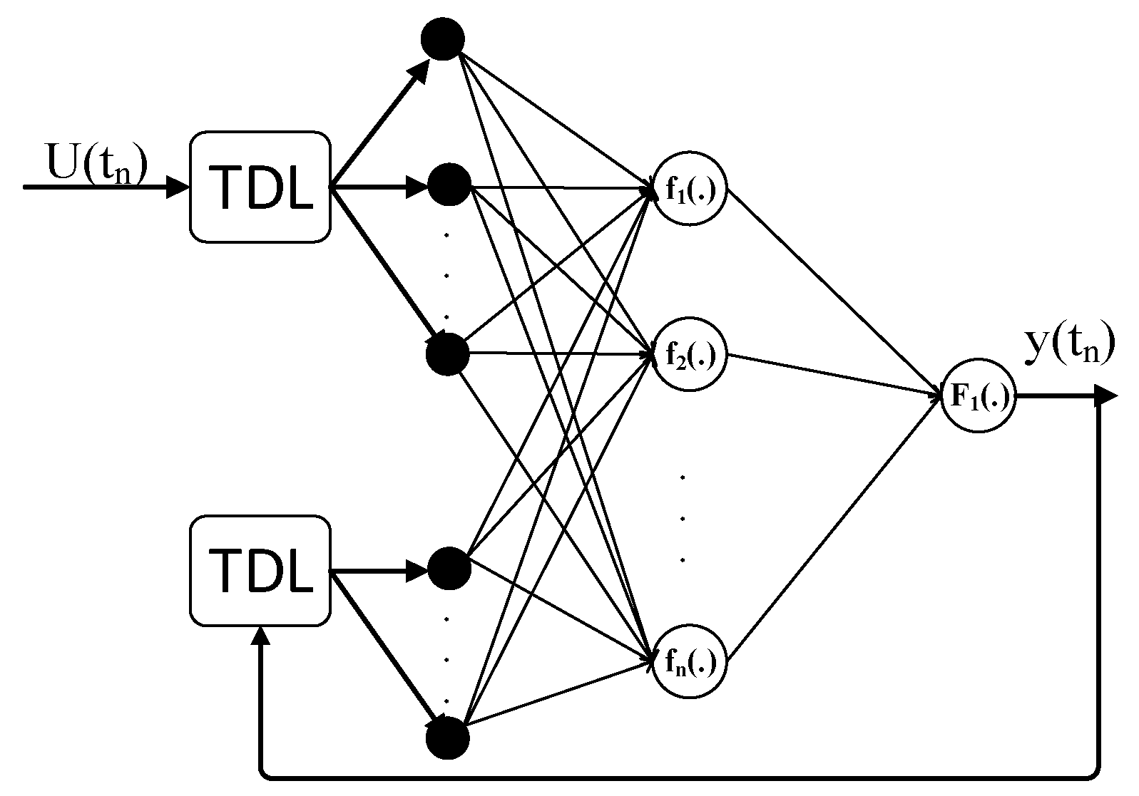
In this expression, refers to the time series output signal, to the exogenous input time series, and and to the time-delay orders of input and output, respectively, which approximate the function . For feedback neural networks, the tapped delay line (TDL) plays the most important role. According to the TDL (Figure 2), the inputs of a neural network are divided into external inputs and delayed external inputs, and the outputs are split into present outputs and delayed outputs. It is assumed that the current predicted value of a time series depends on both the predicted value of the moment before the present moment and the exogenous time series input parameters for the current and previous moments. The existence of the TDL relates the output results to the present input parameters and is the result of interactions between the first input parameter(s) and the first output result(s); the estimation results will not fluctuate due to errors in the current input parameters.
A typical NARX network consists of input, hidden, and output layers and the input and output TDLs. During network training, standardization using input data is required. Moreover, a sigmoidal transformation function should also be used as a transmission function for hidden neurons. To obtain the best result, the suggested number of hidden neurons should not be too large; otherwise, the overfitting phenomenon will occur. To increase training speed, the Levenberg–Marquardt backpropagation algorithm is used to train the neurons.
The overall procedure for using time series to estimate LAI recursively is presented in Figure 2. When the model training data were constructed, the reflectance values in the red and near-infrared (NIR) bands, which are the most sensitive to vegetation growth, were selected as input data. The cosine of the solar zenith angle (SZA), the cosine of the viewing zenith angle (VZA), and the cosine of the relative azimuth (RA) were also taken as the input data. Meanwhile, and , which are the input and output variables of the NARX network, respectively, can be expressed by a time series as follows:
During NARX training, MODIS NABR and MODIS LAI data were used initially to acquire a prior LAI background field at MODIS pixel resolution. For the purpose of trained neural network optimization, data were grouped into training, validation, and testing data at a ratio of 0.7:0.15:0.15. Considering the availability and flexibility of the model, the TDL was set to 0 for the input variables and 1 for the output variables. Equation (1) can be rewritten as follows:
In the methods section, we discuss how to use the recursive update model for HR LAI estimation and address how to create a NARX network and configure the network parameters.
3. Materials
3.1. Study Area
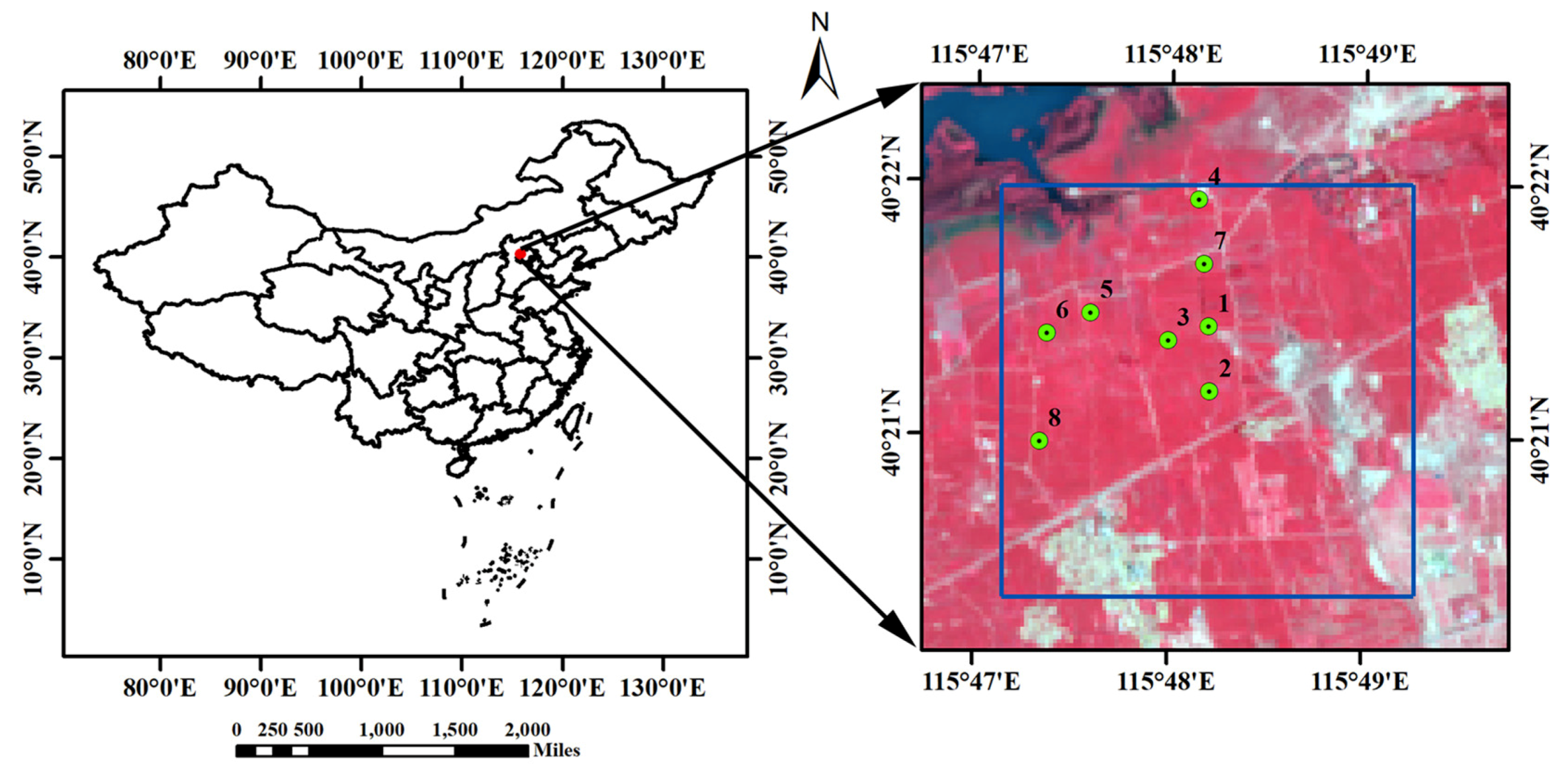
The study area is located in Zhangjiakou City, Huailai County, Hebei Province in northern China (115°80′N, 40°35′E). The study area is a 3 km × 3 km block of farmland, over 90% of which is planted in maize. The land-cover type of the eight ground sites in this area is maize; the LAI values were measured at four sites in 2013 and four sites in 2014. The geographical distribution of the ground measurement sites is shown in Figure 3. The eight sites are located in different MODIS pixels.
3.2. Field Data
A continuous LAI surface observation experiment was performed in the experimental area during the maize-growing season from 2013 to 2014. For the LAI measurements, LAINet was used in 2013, and the LICOR LAI-2000 Plant Canopy Analyzer was used in 2014. LAINet is an automatic device that obtains multi-angle transmittance of the vegetation canopy during the day following the sun’s movement, based on wireless sensor network (WSN) technology, and then calculates the crop LAI from multi-angle transmittance using a vegetation gap probability model. one advantage of LAINet is its ability to provide continuous observations of the vegetation growth process. When the LAI is greater than 3.5, the measured LAINet values may be more accurate than the LAI-2000 values. For the design, the algorithm and validation of LAINet were fully described and tested in previous studies [40,41]. There are four ground samples of measurement during the maize growing season for each year, and the sample size is 30 × 30 m. We selected five points in each sample to perform LAI measurements and took the average to represent the LAI result of the sample. The spatial distribution of the five measurement points consists of four corner points and a center point.
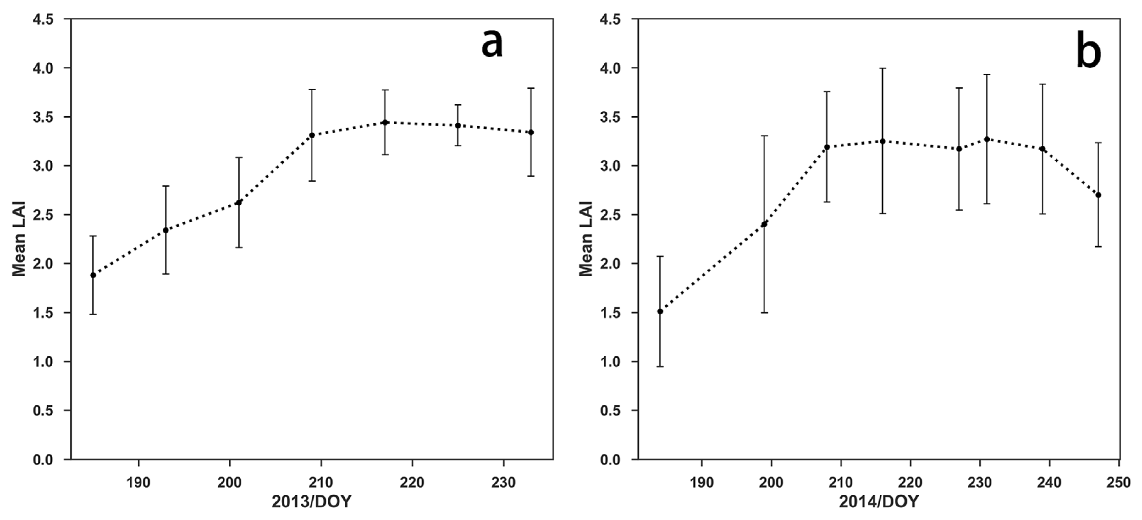
In 2013, the value of the observed sample time series from Julian days 185 to 233 was calculated [42] (Figure 4a). Since the weather changes may cause errors in the measurement results of the LAI, the mean value in the 8-day interval was taken as the LAI value of the sample. In Figure 4a, the dotted black line indicates the LAI timing sequence variations, and the vertical line represents the standard deviation of measurement results for every sampling point. Figure 4a shows a significant growth trend from Julian days 185 to 210; subsequently, the LAI curve gradually becomes flat and stable with a maximum of approximately 3.5.
In 2014, through observations from Julian days 185 to 247 in a single area, the LAI tendency of maize was obtained. From Julian days 185 to 210, the LAI rapidly increased; subsequently, the maximum LAI value was attained, and the LAI gradually became stable at a maximum value near 3; finally, after day 240, the LAI began to decline.
3.3. Satellite Image Pre-Processing
In the study area, large quantities of HJ-1 CCD, GF-1 Wide Field of View (WFV), Landsat 5 Thematic Mapper (TM), Landsat 7 Enhanced Thematic Mapper Plus (ETM+), Landsat 8 Operational Land Imager (OLI), and MODIS surface reflectance data were collected; the available data on the maize growth season are presented in Table 1.
3.3.1. HR Reflectance Data
We used HJ-1, GF-1, and Landsat 5/7/8 observations to produce HR reflectance datasets during 2011–2014. The HJ-1 satellite was launched on September 6, 2008; two CCD cameras with the same design principle were placed symmetrically according to the subsatellite point. The resulting data have a spatial resolution of 30 m. With two CCD cameras, the field of view is divided equally, and observations can be performed in parallel; in addition, push-broom imaging is conducted jointly for four spectrum bands with a swath width of 700 km over the ground. Because the revisit cycle is only four days, a large amount of data can be acquired within a short period. The GF-1 satellite was launched on 26 April 2013; it was the first satellite of the HR Earth observation system in China. The spatial resolution of its multispectral large-width camera is 16 m, and the revisit cycle is two days; in addition, the composite width of its four multispectral image cameras with 16 m resolution is greater than 800 km. Therefore, this satellite has unique advantages for large-scale surface observation and environmental monitoring. These two satellites have the characteristics of HR data and a short revisit cycle and have unique advantages for large-scale surface observation and environmental monitoring. With respect to the revisit cycle, the HJ-1 satellite data are superior to Landsat data, and constructing a long time series dataset is easier with HJ-1 data.
All Landsat 5/7/8 scenes for the study area covering the growing season were acquired through the United States Geological Survey (USGS) (https://earthexplorer.usgs.gov). Landsat 5/7 images were preprocessed using the Landsat Ecosystem Disturbance Adaptive Processing System (LEDAPS) [43]. LEDAPS applies atmospheric correction routines to Landsat TM data, similar to routines derived from MODIS. The Second Simulation of a Satellite Signal in the Solar Spectrum (6S) [44] radiative transfer model was used to generate Landsat surface reflectance. Landsat-8 OLI surface reflectance data are generated from the Landsat Surface Reflectance Code (LaSRC) [45], which is distinctly different with the LEDAPS algorithm. The LaSRC makes use of the coastal aerosol band to perform aerosol inversion tests, uses auxiliary climate data from MODIS and uses a unique radiative transfer model. Landsat 5 Thematic Mapper (TM) operational imaging ended in November 2011. On 31 May 2003, the Scan Line Corrector (SLC), which compensates for the forward motion of the satellite, failed. For the scan line errors of the Landsat 7, we masked the missing data and fill in empty pixels using data from HJ-1 and GF-1 acquired in the same period. Landsat 8 launched on 11 February 2013. The OLI is intended to be broadly compatible with the previous ETM+ bands. At the same time, the OLI bands are refined in order to avoid atmospheric absorption features.
All HJ-1 CCD and GF-1 WFV scenes for the study area were acquired through the China Center for Resources Satellite Data and Application (CRESDA) (http://www.cresda.com). Before constructing the HR datasets, the following steps were applied in the HJ-1 CCD and GF-1 WFV data processing: absolute radiometric calibration, cloud detection, atmospheric correction, and geometric correction.
Absolute calibration parameters provided by CRESDA were also used to carry out radiometric calibration for HJ-1 and GF-1 so that the digital number (DN) value could be translated into apparent reflectance. In this processing, the first step is to convert the DN to spectral radiance . The formula for GF-1 data is
The calibration formula for HJ-1 data is
The apparent reflectance is calculated as
is the band-specific exoatmospheric solar constant, is solar zenith angle, and is the Earth–Sun distance in astronomical units. , and can be found on the website of CRESDA.
Due to the impact of clouds and haze, the surface reflectance changes over the course of a time series; in addition, all data require cloud detection before they can be used to ensure that ground survey sites exhibit clear-sky conditions. This approach ensures that the acquired data represent actual surface physical parameters. Due to the need for cloud detection in HR data, simple indices and thresholding methods must be applied initially to detect thick clouds:
where is the reflectance of the red band and is the reflectance of the NIR band. For the detection results, visual acquisition is used again to determine the presence of clouds and haze. Images that are still contaminated by clouds and haze are discarded.
Atmospheric corrections for HJ-1 and GF-1 satellite data are performed based on the new proposed aerosol retrieval algorithm [46,47] with prior surface reflectance data support. The distributions and surface reflectance of dense pixels are determined using the MOD09 8-day synthetic surface reflectance products to estimate the aerosol contents. Then, these estimates are used as inputs in the 6S radiative transfer model to perform atmospheric correction on every pixel along with precalculated Look-Up Tables (LUTs).
As a level-2 product, the HJ-1 satellite data experience systemic geometric corrections. By comparison, GF-1 is a level-1 product with built-in rational polynomial coefficient (RPC) parameters that must be used to perform coarse geometrical corrections so that geographical coordinate projection can be realized for related images. Level 1 products have experienced only rough geometric correction, and some geometrical errors remain with respect to other remote sensing images. The GF-1 WFV images were resampled to 30 m resolution using the average resampling method to match the HJ-1 CCD data. Because geometric correction at the system level has low positioning precision, high-precision geometric corrections are still required. To rectify GF-1 and HJ-1 satellite data geometrically, Landsat TM data serve as the benchmark, and obvious boundary points such as roads and corners of buildings serve as datum points to implement ground control point (GCP) corrections. Hence, the error in point measurements is within 0.5 pixels.
3.3.2. MCD43A4 NBAR Product
The MCD43A4 version 5 provides 500 m reflectance data adjusted using the bidirectional reflectance distribution function to model the values as if they were collected from a nadir view [48]. The NBAR algorithm produces 8-day composite data using 16-day reflectance data from the Aqua and Terra satellites. Validation at stage 3 has been achieved for the MODIS C5 NBAR product. All images covering the study area were downloaded from The National Aeronautics and Space Administration (NASA) (https://earthdata.nasa.gov). We reprojected the MODIS images to the UTM-WGS84 projection to match the HR reflectance data.
3.3.3. MCD15A2 LAI Product
The MCD15A2 version 6 MODIS LAI product is an 8-day composite dataset with a 500 m pixel size. The algorithms include a main LUT-based procedure and a back-up algorithm based on the LAI-NDVI relationships [49]. Because retrievals of the back-up algorithm have a low quality, this study only used the values retrieved with the main algorithm [50]. The LAI product is considered to be validated to stage 2. MODIS LAI is closer to true LAI than effective LAI and the C6 product is considerably better than C5 [51]. All scenes of MOD15A2 LAI covering the study area were obtained from NASA.
3.3.4. Surface Reflectance Normalization
Within the study area, the primary maize-growing season ranges from Julian days 137 to 257; during this period, the zenith observation angle for the HJ-1, GF-1 and Landsat satellite data usually varies between 0° and 30°, and the satellite passes Huailai between 10:00 AM and 11:00 AM local time every day. The variation in viewing angle will cause apparent change in observed surface reflectance. In order to eliminate the directional effect, we used the method developed by Roy et al. [52] to normalize the high-spatial-resolution surface reflectance to nadir BRDF adjusted reflectance (HR NBAR). So that we can use the MODIS BRDF model parameters (MCD43A1) in the HR NBAR derivation. The data processing technique uses fixed BRDF kernel coefficients for each spectral band derived from a large number of pixels in the BRDF product that are globally and temporally distributed. The technique is very stable, reversible, easy to implement for operational processing [52].
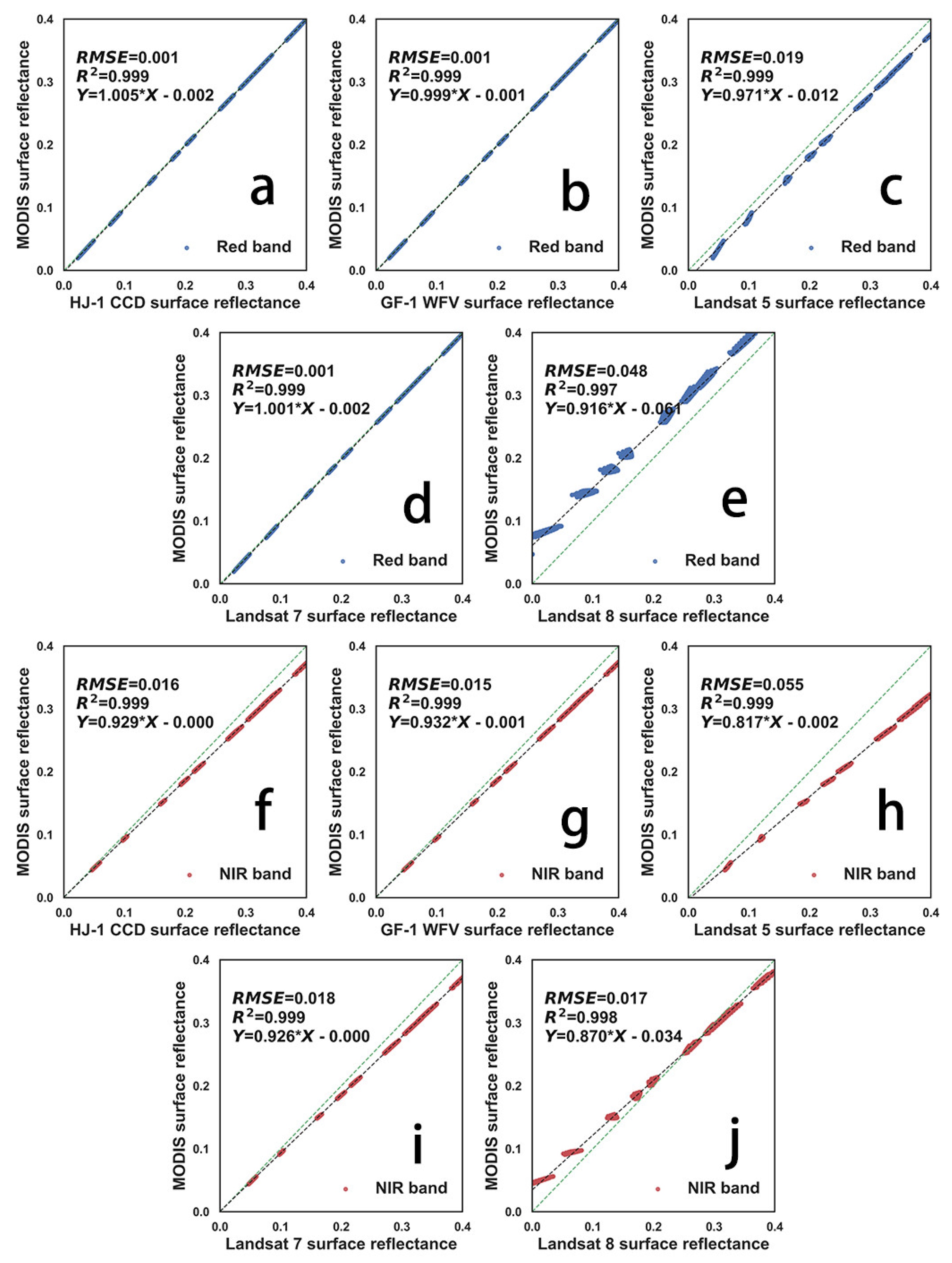
Due to the differences between the spectral response functions of MODIS and the HR sensors, the variation in the surface reflectance is simulated with the 6S radiative transfer model [44] under different geometric observations (SZA, VZA, and RA) and atmospheric conditions. The ranges of parameters used to simulate 6S model are shown in Table 2. The different sensor characters are corrected by comparing the surface reflectance simulated under the same parameters. Figure 5 shows the comparison of HR and MODIS surface reflectance of red and NIR bands.
The NIR band needs to be considered and can be corrected as follows
where and are two linear fitting coefficients, is the surface reflectance of HR data, and is the surface reflectance of MODIS.
The composite method of the HR dataset is based on the generation algorithm of the MOD09 products. For each pixel, a value is selected from all acquisitions within the 8-day composite period. The criterion for the pixel choice is that the HR surface reflectance data are the minimum-blue [53,54]. The surface reflectance values of each of the different bands for the same location and day are copied to the composite image files using minimum blue criteria. The composite HR data not only reduces the inconsistency between the two data due to cloud contamination, but also reduces the difference in reflectance between the data, which facilitates the training of the neural network to retrieve a smooth LAI.
4. Results
4.1. 2013 and 2014 LAI Estimations from Satellite Data
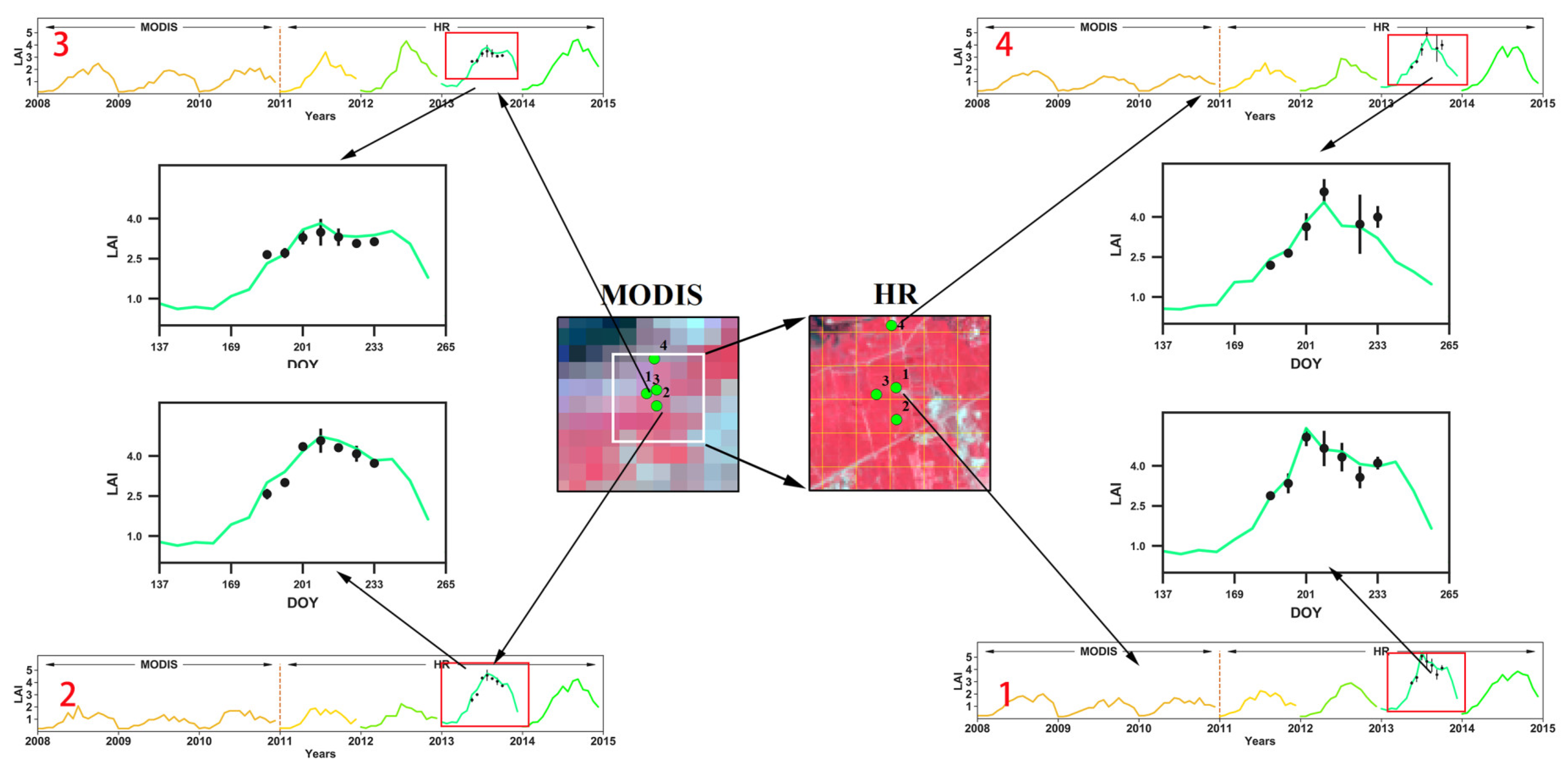
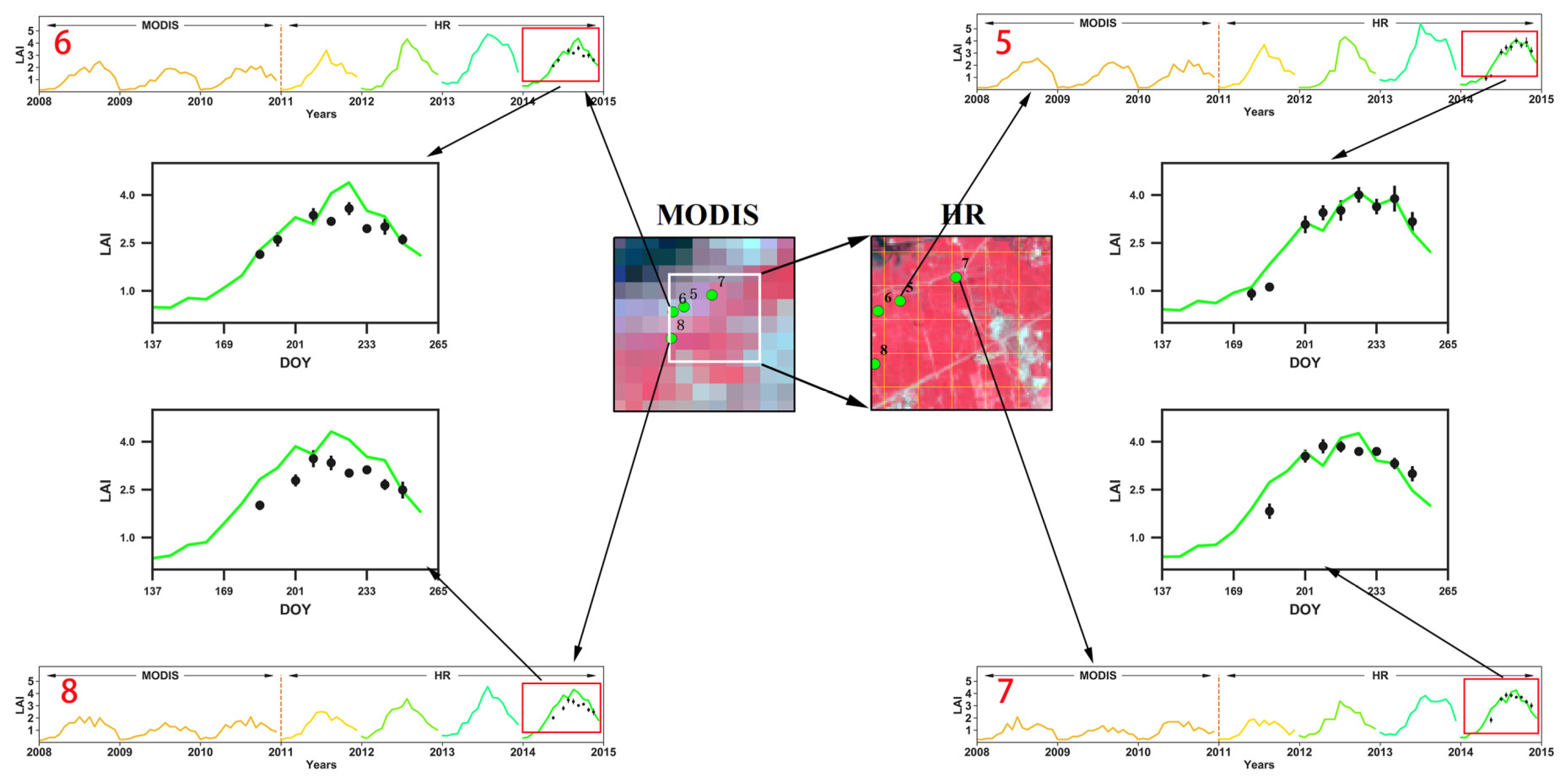
After twice updating the background information of the HR data in the 2011 and 2012 estimation processes, the HR LAI results of 2013 were estimated. The time series comparison between the LAI retrievals from satellite and ground observations at Huailai sites is shown in Figure 6 for 2013 and in Figure 7 for 2014. We note that there is no significant fluctuation in the LAI time series dynamically predicted by the NARX model. The time series from 2008 to 2010 is MODIS LAI data products, and that from 2011 to 2014 is the HR LAI time series.
Figure 6 depicts the LAI time series estimated using our method at the Huailai sites in 2013. The time series from 2008 to 2010 is MODIS LAI products, and that from 2011 to 2014 is the LAI time series retrieved from HR data. The results show the classical temporal pattern for maize, with increasing LAI during the vegetative stage, a peak LAI during the reproductive stage, and a subsequent relatively rapid decline. With the increases in HR data during the estimation process, the LAI appears to be significantly different in the time series. Figure 6 (1–4) shows the temporal trajectories of LAI differences for the 2013 site with the maize crop biome type. The retrieval values, except for those contaminated by residual clouds, are 1 and 2 LAI units higher than the MODIS values during the reproductive stage. In Figure 6, the accuracy of the LAI estimation in the reproductive stages is slightly lower than in the other vegetation stages. The possible reason is that the retrieval results are inaccurate due to the image being covered by clouds during the maturity of the corn.
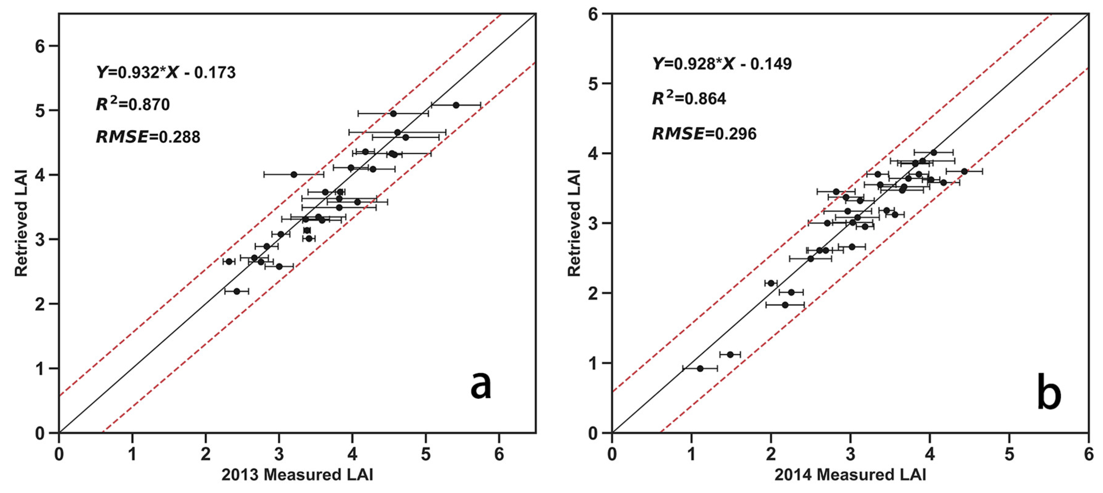
Direct comparisons of the ground measurements from LAINet and the retrieval LAI values demonstrate that the NARX method provides good performance for the HR data in 2013 ( = 0.87 and RMSE = 0.288) and in 2014 ( = 0.864 and RMSE = 0.296). Most LAINet measurements have a small standard deviation, but there are a few data with very large deviations, and the standard deviation of the LAI-2000 measurements is relatively consistent. The LAINet is an automatic measuring device that may cause large deviations in certain results during the measurement process due to weather. The average of multiple measurements will weaken the error, preventing it from having a significant impact on the final verification result. It can be seen in Figure 8 that the mean of the measurements is substantially within the 95% confidence interval.
4.2. Regional LAI Estimation
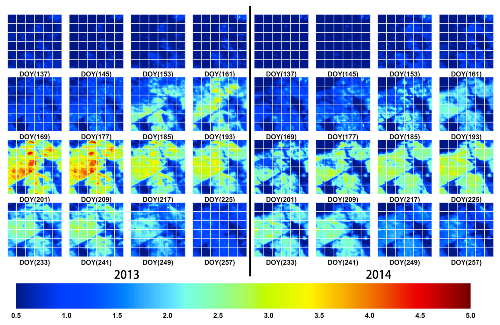
To test the applicability of the NARX model, it was further used for HR LAI estimation in the Huailai study region (blue box in Figure 3). In this way, the 2013–2014 LAI retrieval results for this region were acquired, as shown in Figure 9. The size of each white cell is 500 m × 500 m, which is the MODIS pixel resolution. These figures show that more detail can be achieved at HR satellite pixel resolution; for MODIS pixel resolution, the area of one MODIS pixel is approximately equal to the area of 272 HR pixels. In the case where land-cover types of the sample region are consistent, with flat terrain and weak heterogeneity, for instance, the retrieval results at MODIS pixel resolution can be representative. In real-world situations, the probability of such a large-scale uniform surface is low. However, at a spatial resolution of 30 m, most regions can be considered pure pixels, unlike the coarse 500 m resolution MODIS images. On the MODIS pixel scale, the mixed-pixel phenomenon is much more serious than in the HR dataset. Although the background field is MODIS-scale, the surface reflectance of HR data served as the input parameter during estimation, the spatial resolution of the HR data is higher than MODIS data so that the differences in the results obtained through relevant predictions for the same background pixel would present the characteristics of HR data. Based on spatial resolution retrieval results for the regions shown in Figure 9, the entire LAI set of retrieval results for the Huailai area conforms to the tendencies of the measured data. The LAI reached its maximum on the 201st day of 2013 and on the 217th day of 2014.
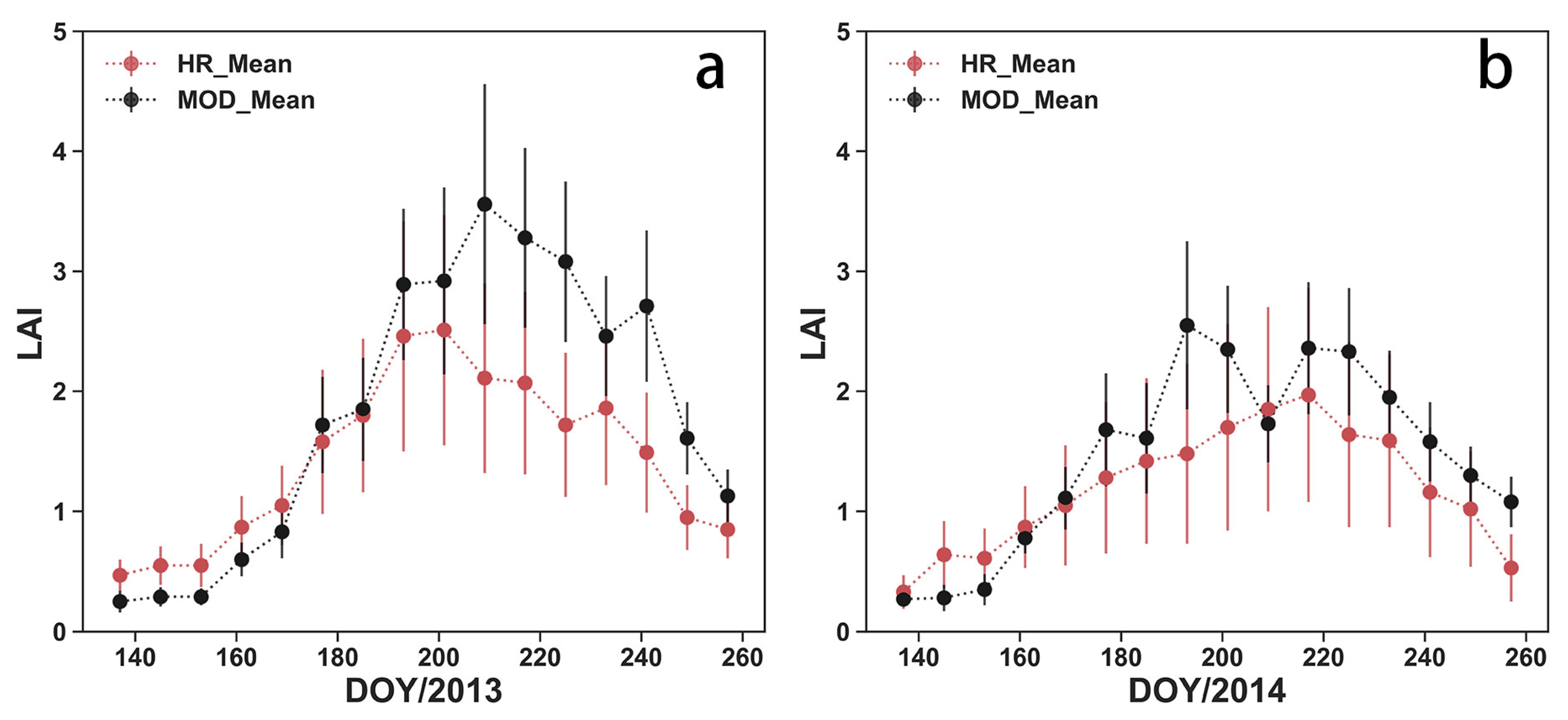
In the HR regional results and the MODIS data for the same region, the edges of the Guanting Reservoir are shown in the upper left corner, but other areas without vegetation coverage are denoted by invalid values in the MODIS data, which occupy approximately one-half of the entire region. For these invalid values, we use the model constructed by the nearest pixel to retrieval the LAI value. In the comparisons of regional retrieval results, more in accordance with the phenological patterns of maize LAI. In Figure 10, MODIS LAI exhibited a very large jump on day 209 of 2014, it may be due to estimation errors caused by clouds or shadows. For the HR dataset retrieval results, even though fluctuations occurred in the input surface reflectance, leading to variations in the LAI, the feedback action of NARX enabled the LAI retrieval results to remain within a reasonable range, without error accumulations caused by chain reactions. Compared with fluctuations in MODIS, HR results have improved this situation. This capability indicates that the NARX neural network has extremely strong fault tolerance. Moreover, for the HR retrieval results, with changes in the day of the year (DOY), no significant fluctuation occurs, and these data effectively conform to surface measurement results.
5. Discussion
In this research, MODIS, NBAR, and LAI time series from 2008 to 2010 were used as background information to calculate the initial parameters of the NARX neural network. Then, HR observation data of 2011 were input into the trained neural network to estimate HR LAI data for 2011, and both MODIS and HR data were used to update the parameters of the NARX neural network, which was then used as the background to estimate the 2012 LAI. This procedure is recursively repeated year by year until both MODIS background data and all HR data were involved in the training.
The empirical model has high precision in specific regions, but the model seems to lack generic capacity and may not be applicable to other areas, and radiative transfer models are mostly under-determined and ill-posed. The number of unknowns is typically much larger than the number of independent observations [55]. For the estimation of surface parameters with obvious annual cycle variation characteristics, such as LAI, the variation characteristics can be extracted from a long-term low-resolution dataset. It can be used as supplementary material for HR observation data and constrained inversion for LAI. At the same time, our recursive update method effectively solves the difference between low-resolution background data and high-resolution sub-pixels, which can effectively improve the estimation accuracy of HR LAI. Compared to the empirical and radiative transfer models, meanwhile, our model combining low-resolution images and high-resolution images with machine learning algorithms. The recursive update model only requires multiyear low-resolution background data, sequential variation in the data from low-resolution LAI products were used as a reference for HR LAI estimation, and HR LAI retrieval can be conducted on this basis. Due to the characteristics of the NARX neural network, the model has a strong capacity for fault tolerance to the input data, the noise in the HR surface reflectance data can be effectively suppressed. The estimation results are more consistent with the phenological changes of maize LAI. In this paper, estimating the HR LAI using the NARX model can be considered a semi-physical model, because the background data is obtained by inversion using the radiative transfer model. Compared with the downscaling and data fusion method, the method in this paper has obvious differences. Coarse resolution data need to be used only in the early stages of the estimation process to provide background information support, and all subsequent estimations are performed using high spatial resolution data. The general neural network algorithm requires pure pixels for training in the estimation process, but our method does not require pure pixels. During the training process, the background information is extracted based on the growth information of each pixel. The recursive updating model is insensitive to the outliers in the observed data. This will not cause errors in the estimation results due to fluctuations in a certain period of time in the pixel. The comparison of the model estimation results with the ground measurements demonstrates that the two results show relatively good consistency. Compared with the results without BRDF correction, the accuracy of the estimation results is significantly improved after the BRDF correction. Previous research has shown that MODIS BRDF spectral parameters can be used to reduce the BRDF effects of high spatial resolution data [56,57,58].
However, due to the limitations of HR satellite data, such as those for HJ-1, in the neural network training process, the input parameters included only the reflectance of the red and NIR bands, which are fairly sensitive to vegetation. If shortwave infrared bands are measured by satellites, these data can be introduced as a modification to counteract satellite data noise. Due to the HR data having a high spatial resolution, minor deviation in geometric positioning can generate substantial errors. Therefore, precise geometric corrections are required during initial processing. Although the retrieval model presented here has achieved good results in croplands, applications in other land types need to be further validated. Moreover, the quality of the training samples has a serious impact on the estimation results, MODIS over-estimating LAI in sparse vegetation areas and underestimating LAI in dense vegetation areas [59] and the effect of using MODIS LAI as a training sample on the results needs further analysis. The NARX neural network needs to be trained for the time series of each pixel, it will take a long time to estimate in a large area. On average, it took about 8 minutes of training time for 300 × 300-pixel image size. The time was measured on a computer with Intel Core i7 3.4 GHz processor and 4 GB of random access memory (RAM). We will try to improve the algorithm and shorten the training time.
6. Conclusions
In this study, HR satellite data with short revisit intervals are used to predict high spatial resolution LAI values over the area of the Huailai experimental region in Hebei Province, China. A historical low-resolution MODIS product was used as background information to extract the stable phenological changes in vegetation, which were used to estimate the HR LAI. The HR data and low-resolution data are then used for recursive update training, resulting in LAI data with a spatial resolution of 30 m. This study demonstrated the feasibility of frequent observations at high spatial resolution for crop monitoring. The estimation results of our proposed recursive update model are compared with ground-measured data, and the two show good consistency. The results demonstrate that the new method can produce temporally continuous and smooth LAI profiles from HR time series observations. The main advantage of the recursive approach is the ability to update model dynamics. Additional studies should be conducted to improve phenological information extraction and disturbance detection in subsequent dynamic monitoring. With the increase in HR remote sensing data, we will further study the method of normalizing multisource remote sensing data, and we plan to obtain high-precision surface reflectance data and to improve the accuracy of the time series estimation of LAI.
Author Contributions
J.W. (Jindi Wang) conceived and designed the study. J.W. (Jian Wang) contributed to the conception of the study, performed the data analysis, and wrote the paper. Y.S., H.Z. and L.L. aided with the discussion and the manuscript revision. J.W. (Jindi Wang) reviewed and edited the manuscript. All authors read and approved the manuscript.
Acknowledgments
This research was supported by the National Basic Research Program of China under grant No.2013CB733403, the National Natural Science Foundation of China under grant No. 41171263, and the National Natural Science Foundation of China under grant No. 41801242.
Conflicts of Interest
The authors declare no conflict of interest.
References
- Chen, J.M.; Black, T. Defining leaf area index for non-flat leaves. Plant Cell Environ. 1992, 15, 421–429. [Google Scholar] [CrossRef]
- Hernández, C.; Nunes, L.; Lopes, D.; Graña, M. Data fusion for high spatial resolution lai estimation. Inf. Fusion 2014, 16, 59–67. [Google Scholar] [CrossRef]
- Bsaibes, A.; Courault, D.; Baret, F.; Weiss, M.; Olioso, A.; Jacob, F.; Hagolle, O.; Marloie, O.; Bertrand, N.; Desfond, V. Albedo and lai estimates from formosat-2 data for crop monitoring. Remote Sens. Environ. 2009, 113, 716–729. [Google Scholar] [CrossRef]
- Chern, J.-S.; Wu, A.-M.; Lin, S.-F. Lesson learned from formosat-2 mission operations. Acta Astronaut. 2006, 59, 344–350. [Google Scholar] [CrossRef]
- Pu, R.; Cheng, J. Mapping forest leaf area index using reflectance and textural information derived from worldview-2 imagery in a mixed natural forest area in Florida, US. Int. J. Appl. Earth Obs. Geoinf. 2015, 42, 11–23. [Google Scholar] [CrossRef]
- Verrelst, J.; Rivera, J.P.; Veroustraete, F.; Muñoz-Marí, J.; Clevers, J.G.P.W.; Camps-Valls, G.; Moreno, J. Experimental sentinel-2 lai estimation using parametric, non-parametric and physical retrieval methods—A comparison. ISPRS J. Photogramm. Remote Sens. 2015, 108, 260–272. [Google Scholar] [CrossRef]
- Novelli, A.; Tarantino, E.; Fratino, U.; Iacobellis, V.; Romano, G.; Gentile, F. A data fusion algorithm based on the kalman filter to estimate leaf area index evolution in durum wheat by using field measurements and modis surface reflectance data. Remote Sens. Lett. 2016, 7, 476–484. [Google Scholar] [CrossRef]
- Eklundh, L.; Hall, K.; Eriksson, H.; Ardö, J.; Pilesjö, P. Investigating the use of landsat thematic mapper data for estimation of forest leaf area index in southern sweden. Can. J. Remote Sens. 2003, 29, 349–362. [Google Scholar] [CrossRef]
- Baret, F.; Clevers, J.; Steven, M. The robustness of canopy gap fraction estimates from red and near-infrared reflectances: A comparison of approaches. Remote Sens. Environ. 1995, 54, 141–151. [Google Scholar] [CrossRef]
- Walthall, C.; Dulaney, W.; Anderson, M.; Norman, J.; Fang, H.; Liang, S. A comparison of empirical and neural network approaches for estimating corn and soybean leaf area index from landsat etm+ imagery. Remote Sens. Environ. 2004, 92, 465–474. [Google Scholar] [CrossRef]
- Potithep, S.; Nasahara, K.; Muraoka, H.; Nagai, S.; Suzuki, R. What is the actual relationship between lai and vi in a deciduous broadleaf forest? Int. Arch. Photogramm. Remote Sens. Spat. Inf. Sci. 2010, 38, 609–614. [Google Scholar]
- Fan, L.; Gao, Y.; Brück, H.; Bernhofer, C. Investigating the relationship between ndvi and lai in semi-arid grassland in inner mongolia using in-situ measurements. Theor. Appl. Climatol. 2009, 95, 151–156. [Google Scholar] [CrossRef]
- Lee, B.; Kwon, H.; Miyata, A.; Lindner, S.; Tenhunen, J. Evaluation of a phenology-dependent response method for estimating leaf area index of rice across climate gradients. Remote Sens. 2016, 9, 20. [Google Scholar] [CrossRef]
- Darvishzadeh, R.; Skidmore, A.; Schlerf, M.; Atzberger, C. Inversion of a radiative transfer model for estimating vegetation lai and chlorophyll in a heterogeneous grassland. Remote Sens. Environ. 2008, 112, 2592–2604. [Google Scholar] [CrossRef]
- Schlerf, M.; Atzberger, C. Inversion of a forest reflectance model to estimate structural canopy variables from hyperspectral remote sensing data. Remote Sens. Environ. 2006, 100, 281–294. [Google Scholar] [CrossRef]
- Weiss, M.; Baret, F.; Myneni, R.; Pragnère, A.; Knyazikhin, Y. Investigation of a model inversion technique to estimate canopy biophysical variables from spectral and directional reflectance data. Agronomie 2000, 20, 3–22. [Google Scholar] [CrossRef]
- Meroni, M.; Colombo, R.; Panigada, C. Inversion of a radiative transfer model with hyperspectral observations for lai mapping in poplar plantations. Remote Sens. Environ. 2004, 92, 195–206. [Google Scholar] [CrossRef]
- Combal, B.; Baret, F.; Weiss, M.; Trubuil, A.; Mace, D.; Pragnere, A.; Myneni, R.; Knyazikhin, Y.; Wang, L. Retrieval of canopy biophysical variables from bidirectional reflectance: Using prior information to solve the ill-posed inverse problem. Remote Sens. Environ. 2003, 84, 1–15. [Google Scholar] [CrossRef]
- Durbha, S.S.; King, R.L.; Younan, N.H. Support vector machines regression for retrieval of leaf area index from multiangle imaging spectroradiometer. Remote Sens. Environ. 2007, 107, 348–361. [Google Scholar] [CrossRef]
- Pan, J. Retrieve leaf area index from hj-ccd image based on support vector regression and physical model. Proc. SPIE 2013, 8887, 88871R. [Google Scholar]
- Tang, H.; Brolly, M.; Zhao, F.; Strahler, A.H.; Schaaf, C.L.; Ganguly, S.; Zhang, G.; Dubayah, R. Deriving and validating leaf area index (lai) at multiple spatial scales through lidar remote sensing: A case study in sierra national forest, ca. Remote Sens. Environ. 2014, 143, 131–141. [Google Scholar] [CrossRef]
- Shi, Y.; Wang, J.; Qin, J.; Qu, Y. An upscaling algorithm to obtain the representative ground truth of lai time series in heterogeneous land surface. Remote Sens. 2015, 7, 12887–12908. [Google Scholar] [CrossRef]
- Danson, F.M.; Rowland, C.S.; Baret, F. Training a neural network with a canopy reflectance model to estimate crop leaf area index. Int. J. Remote Sens. 2003, 24, 4891–4905. [Google Scholar] [CrossRef]
- Noble, P.A.; Tribou, E.H. Neuroet: An easy-to-use artificial neural network for ecological and biological modeling. Ecol. Model. 2007, 203, 87–98. [Google Scholar] [CrossRef]
- Li, Z.; Fox, J.M. Integrating mahalanobis typicalities with a neural network for rubber distribution mapping. Remote Sens. Lett. 2011, 2, 157–166. [Google Scholar] [CrossRef]
- Shupe, S.M.; Marsh, S.E. Cover-and density-based vegetation classifications of the sonoran desert using landsat tm and ers-1 sar imagery. Remote Sens. Environ. 2004, 93, 131–149. [Google Scholar] [CrossRef]
- Jensen, J.; Qiu, F.; Ji, M. Predictive modelling of coniferous forest age using statistical and artificial neural network approaches applied to remote sensor data. Int. J. Remote Sens. 1999, 20, 2805–2822. [Google Scholar]
- Muukkonen, P.; Heiskanen, J. Estimating biomass for boreal forests using aster satellite data combined with standwise forest inventory data. Remote Sens. Environ. 2005, 99, 434–447. [Google Scholar] [CrossRef]
- Bacour, C.; Baret, F.; Béal, D.; Weiss, M.; Pavageau, K. Neural network estimation of lai, fapar, fcover and lai×cab, from top of canopy meris reflectance data: Principles and validation. Remote Sens. Environ. 2006, 105, 313–325. [Google Scholar] [CrossRef]
- Fang, H.; Liang, S. Retrieving leaf area index with a neural network method: Simulation and validation. IEEE Trans. Geosci. Remote Sens. 2003, 41, 2052–2062. [Google Scholar] [CrossRef]
- Fang, H.; Liang, S. A hybrid inversion method for mapping leaf area index from modis data: Experiments and application to broadleaf and needleleaf canopies. Remote Sens. Environ. 2005, 94, 405–424. [Google Scholar] [CrossRef]
- Gao, F.; Masek, J.; Schwaller, M.; Hall, F. On the blending of the landsat and modis surface reflectance: Predicting daily landsat surface reflectance. IEEE Trans. Geosci. Remote Sens. 2006, 44, 2207–2218. [Google Scholar]
- Liu, Y.; Wang, X.; Liu, Y. Asynchronous harmonic analysis based on out-of-sequence measurement for large-scale residential power network. In Proceedings of the Instrumentation and Measurement Technology Conference, Pisa, Italy, 11–14 May 2015; pp. 1693–1698. [Google Scholar]
- Baghaee, H.R.; Mirsalim, M.; Gharehpetan, G.B.; Talebi, H.A. Nonlinear load sharing and voltage compensation of microgrids based on harmonic power-flow calculations using radial basis function neural networks. IEEE Syst. J. 2016, PP, 1–11. [Google Scholar] [CrossRef]
- Wunsch, A.; Liesch, T.; Broda, S. Forecasting groundwater levels using nonlinear autoregressive networks with exogenous input (narx). J. Hydrol. 2018, 567, 743–758. [Google Scholar] [CrossRef]
- Sauter, T.; Weitzenkamp, B.; Schneider, C. Spatio-temporal prediction of snow cover in the black forest mountain range using remote sensing and a recurrent neural network. Int. J. Climatol. 2010, 30, 2330–2341. [Google Scholar] [CrossRef]
- Chai, L.; Qu, Y.; Zhang, L.; Liang, S.; Wang, J. Estimating time-series leaf area index based on recurrent nonlinear autoregressive neural networks with exogenous inputs. Int. J. Remote Sens. 2012, 33, 5712–5731. [Google Scholar] [CrossRef]
- Lin, T.; Horne, B.G.; Tino, P.; Giles, C.L. Learning long-term dependencies in narx recurrent neural networks. IEEE Trans. Neural Netw. 1996, 7, 1329–1338. [Google Scholar] [PubMed]
- Demuth, H.; Beale, M. Neural Network Toolbox for Use with Matlab; Mathworks Inc.: Natick, MA, USA, 1992; p. 355. [Google Scholar]
- Qu, Y.; Han, W.; Fu, L.; Li, C.; Song, J.; Zhou, H.; Bo, Y.; Wang, J. Lainet—A wireless sensor network for coniferous forest leaf area index measurement: Design, algorithm and validation. Comput. Electron. Agric. 2014, 108, 200–208. [Google Scholar] [CrossRef]
- Qu, Y.; Zhu, Y.; Han, W.; Wang, J.; Ma, M. Crop leaf area index observations with a wireless sensor network and its potential for validating remote sensing products. IEEE J. Sel. Top. Appl. Earth Obs. Remote Sens. 2014, 7, 431–444. [Google Scholar] [CrossRef]
- Shi, Y.; Wang, J.; Wang, J.; Qu, Y. A prior knowledge-based method to derivate high-resolution leaf area index maps with limited field measurements. Remote Sens. 2016, 9, 13. [Google Scholar] [CrossRef]
- Masek, J.G.; Vermote, E.F.; Saleous, N.E.; Wolfe, R.; Hall, F.G.; Huemmrich, K.F.; Gao, F.; Kutler, J.; Lim, T.K. A landsat surface reflectance dataset for north america, 1990–2000. IEEE Geosci. Remote Sens. Lett. 2006, 3, 68–72. [Google Scholar] [CrossRef]
- Vermote, E.F.; Tanre, D.; Deuze, J.L.; Herman, M.; Morcette, J.J. Second Simulation of the Satellite Signal in the Solar Spectrum, 6S: an overview. IEEE Trans. Geosci. Remote Sens. 1997, 35, 675–686. [Google Scholar] [CrossRef]
- Vermote, E.; Justice, C.; Claverie, M.; Franch, B. Preliminary analysis of the performance of the landsat 8/oli land surface reflectance product. Remote Sens. Environ. 2016, 185, 46–56. [Google Scholar] [CrossRef]
- Sun, L.; Wei, J.; Bilal, M.; Tian, X.; Jia, C.; Guo, Y.; Mi, X. Aerosol optical depth retrieval over bright areas using landsat 8 oli images. Remote Sens. 2015, 8, 23. [Google Scholar] [CrossRef]
- Sun, L.; Sun, C.; Liu, Q.; Zhong, B. Aerosol optical depth retrieval by hj-1/ccd supported by modis surface reflectance data. Sci. China Earth Sci. 2010, 53, 74–80. [Google Scholar] [CrossRef]
- Schaaf, C.B.; Gao, F.; Strahler, A.H.; Lucht, W.; Li, X.; Tsang, T.; Strugnell, N.C.; Zhang, X.; Jin, Y.; Muller, J.P. First operational brdf, albedo nadir reflectance products from modis. Remote Sens. Environ. 2002, 83, 135–148. [Google Scholar] [CrossRef]
- Myneni, R.B.; Hoffman, S.; Knyazikhin, Y.; Privette, J.L.; Glassy, J.; Tian, Y.; Wang, Y.; Song, X.; Zhang, Y.; Smith, G.R. Global products of vegetation leaf area and fraction absorbed par from year one of modis data. Remote Sens. Environ. 2002, 83, 214–231. [Google Scholar] [CrossRef]
- Yang, W.; Huang, D.; Tan, B.; Stroeve, J.C.; Shabanov, N.V.; Knyazikhin, Y.; Nemani, R.R.; Myneni, R.B. Analysis of leaf area index and fraction of par absorbed by vegetation products from the terra modis sensor: 2000–2005. IEEE Trans. Geosci. Remote Sens. 2006, 44, 1829–1842. [Google Scholar] [CrossRef]
- Yan, K.; Park, T.; Yan, G.; Liu, Z.; Yang, B.; Chen, C.; Nemani, R.R.; Knyazikhin, Y.; Myneni, R.B. Evaluation of modis lai/fpar product collection 6. Part 2: Validation and intercomparison. Remote Sens. 2016, 8, 460. [Google Scholar] [CrossRef]
- Roy, D.P.; Zhang, H.K.; Ju, J.; Gomez-Dans, J.L.; Lewis, P.E.; Schaaf, C.B.; Sun, Q.; Li, J.; Huang, H.; Kovalskyy, V. A general method to normalize landsat reflectance data to nadir brdf adjusted reflectance. Remote Sens. Environ. 2016, 176, 255–271. [Google Scholar] [CrossRef]
- Vermote, E.; Vermeulen, A. Atmospheric Correction Algorithm: Spectral Reflectances (mod09), Algorithm Theoretical Background Document. 1999; version 4.0. Available online: https://lpdaac.usgs.gov/sites/default/files/public/product_documentation/atbd_mod09.pdf (accessed on 28 January 2019).
- Descloitres, J.; Vermote, E. Operational retrieval of the spectral surface reflectance and vegetation index at global scale from seawifs data. International Conference on Aerosols, Radiation Budget–Land Surfaces–Ocean Colour: The Contribution of POLDER and New Generation Spaceborne Sensors to Global Change Studies; Land Surfaces-O-02; CNES: Meribel, France; Toulouse, France, 1999; pp. 1–4.
- Verrelst, J.; Camps-Valls, G.; Muñoz-Marí, J.; Rivera, J.P.; Veroustraete, F.; Clevers, J.G.P.W.; Moreno, J. Optical remote sensing and the retrieval of terrestrial vegetation bio-geophysical properties—A review. ISPRS J. Photogramm. Remote Sens. 2015, 108, 273–290. [Google Scholar] [CrossRef]
- Roy, D.P.; Ju, J.; Lewis, P.; Schaaf, C.; Gao, F.; Hansen, M.; Lindquist, E. Multi-temporal modis–landsat data fusion for relative radiometric normalization, gap filling, and prediction of landsat data. Remote Sens. Environ. 2008, 112, 3112–3130. [Google Scholar] [CrossRef]
- Li, F.; Jupp, D.L.B.; Reddy, S.; Lymburner, L.; Mueller, N.; Tan, P.; Islam, A. An evaluation of the use of atmospheric and brdf correction to standardize landsat data. IEEE J. Sel. Top. Appl. Earth Obs.Remote Sens. 2010, 3, 257–270. [Google Scholar] [CrossRef]
- Feng, G.; Tao, H.; Masek, J.; Shuai, Y.; Wang, Z. Angular effects and correction for medium resolution sensors to support crop monitoring. IEEE J. Sel. Top. Appl. Earth Obs. Remote Sens. 2014, 7, 4480–4489. [Google Scholar]
- Garrigues, S.; Lacaze, R.; Baret, F.; Morisette, J.T.; Weiss, M.; Nickeson, J.E.; Fernandes, R.; Plummer, S.; Shabanov, N.V.; Myneni, R.B. Validation and intercomparison of global leaf area index products derived from remote sensing data. J. Geophys. Res. Biogeosci. 2015, 113. [Google Scholar] [CrossRef]
Figure 1.
A flowchart for the Nonlinear Auto-Regressive with Exogenous Inputs (NARX) network-based recursive update model to estimate Leaf area index (LAI). D and M in the plots stand for training data and the NARX network, respectively. (1), (2), …(i) represent the training step number. The green dotted box represents step 1. The red dotted box represents step 2. The blue dotted box represents step 3.

Figure 2.
Architecture of the NARX network configured with tapped delay lines (TDLs).

Figure 3.
The location of Huailai in Hebei Province, China, and eight field sample locations overlaid on a false-color Landsat Thematic Mapper (TM) image.
Figure 3.
The location of Huailai in Hebei Province, China, and eight field sample locations overlaid on a false-color Landsat Thematic Mapper (TM) image.

Figure 4.
Temporal variation in mean LAI at the Huailai sites. The error bars are the standard deviation: (a) The measuring instrument in 2013 was LAINet. (b) The measuring instrument in 2014 was LAI-2000.
Figure 4.
Temporal variation in mean LAI at the Huailai sites. The error bars are the standard deviation: (a) The measuring instrument in 2013 was LAINet. (b) The measuring instrument in 2014 was LAI-2000.

Figure 5.
The relationships between Moderate Resolution Imaging Spectroradiometer (MODIS) surface reflectance and high resolution (HR) surface reflectance in the red and near-infrared (NIR) bands. (a–e) Surface reflectance in the red band; (f–j) surface reflectance in the NIR band.
Figure 5.
The relationships between Moderate Resolution Imaging Spectroradiometer (MODIS) surface reflectance and high resolution (HR) surface reflectance in the red and near-infrared (NIR) bands. (a–e) Surface reflectance in the red band; (f–j) surface reflectance in the NIR band.

Figure 6.
LAI dynamics derived from HR data using NARX prediction over the study sites and comparison with ground-measured LAI values by LAINet. 1–4 are the four ground sites in 2013. Mean values derive from multiple measurements by the LAINet instrument. Error bars indicate standard deviations of the LAINet measurements.

Figure 7.
LAI dynamics derived from HR data using NARX prediction over the study sites and comparison with ground-measured LAI values by LAI-2000. 5–8 are the four ground sites in 2014. Mean values derive from multiple measurements by the LAI-2000 instrument. Error bars indicate standard deviations of the LAI-2000 measurements.

Figure 8.
Comparison between the HR LAI retrievals and ground measurements, which in 2013 were derived from (a) LAINet and in 2014 were derived from (b) LAI-2000. The error bars represent the standard deviation of the ground measurements from LAI instrument. The black solid line is the 1:1 reference line, while the red dotted lines show the 95% confidence interval around the NARX model’s estimate.

Figure 9.
Spatiotemporal LAI maps of the Huailai area in 2013 and 2014 (100 × 100 pixels, 30 m spatial resolution) predicted by the NARX model.
Figure 9.
Spatiotemporal LAI maps of the Huailai area in 2013 and 2014 (100 × 100 pixels, 30 m spatial resolution) predicted by the NARX model.

Figure 10.
Time series comparison between the mean of the LAI at Huailai and the corresponding LAI of the MODIS product: (a) 2013, (b) 2014. The error bars represent the standard deviation from the MODIS LAI product (black) and the retrieved LAI (red).
Figure 10.
Time series comparison between the mean of the LAI at Huailai and the corresponding LAI of the MODIS product: (a) 2013, (b) 2014. The error bars represent the standard deviation from the MODIS LAI product (black) and the retrieved LAI (red).


Table 1.
Summary of different types of satellite images used in Huailai.
| Data | Band | Spectral (nm) | Spatial (m) | Temporal (day) | Year | Images for Huailai |
|---|---|---|---|---|---|---|
| HJ-1 CCD | Red | 630–690 | 30 | 4 | 2011 | 31 |
| 2012 | 25 | |||||
| NIR | 760–900 | 2013 | 40 | |||
| 2014 | 26 | |||||
| GF-1 WFV | Red | 630–690 | 16 | 2 | 2013 | 9 |
| NIR | 770–890 | 2014 | 8 | |||
| Landsat 5 TM | Red | 630–690 | 30 | 16 | 2011 | 7 |
| NIR | 760–900 | |||||
| Landsat 7 ETM+ | Red | 630–690 | 30 | 16 | 2012 | 6 |
| NIR | 770–900 | |||||
| Landsat 8 OLI | Red | 640–670 | 30 | 16 | 2013 | 6 |
| NIR | 850–880 | 2014 | 8 | |||
| MCD43A4 | Red | 620–670 | 500 | 8 | 2008 | 12 |
| 2009 | 12 | |||||
| NIR | 841–876 | |||||
| 2010 | 12 | |||||
| MCD15A2 | - | - | 500 | 8 | 2008 | 12 |
| 2009 | 12 | |||||
| 2010 | 12 |
Table 2.
List of variables required to 6S model and their ranges.
| Parameter Description | Parameter Name | Range |
|---|---|---|
| geometrical conditions | Solar zenith angle | 20–60 (°) |
| Satellite zenith angle | 20–60 (°) | |
| Relative azimuth angle | 0–180 (°) | |
| atmospheric model | Midlatitude summer | - |
| Midlatitude winter | - | |
| aerosol model | continental model | - |
| urban model | - | |
| aerosol optical depth | aerosol optical depth at 550 | 0–1 |
| reflectance | TOA | 0–0.5 |
© 2019 by the authors. Licensee MDPI, Basel, Switzerland. This article is an open access article distributed under the terms and conditions of the Creative Commons Attribution (CC BY) license (http://creativecommons.org/licenses/by/4.0/).
Share and Cite
MDPI and ACS Style
Wang, J.; Wang, J.; Shi, Y.; Zhou, H.; Liao, L. A Recursive Update Model for Estimating High-Resolution LAI Based on the NARX Neural Network and MODIS Times Series. Remote Sens. 2019, 11, 219. https://doi.org/10.3390/rs11030219
AMA Style
Wang J, Wang J, Shi Y, Zhou H, Liao L. A Recursive Update Model for Estimating High-Resolution LAI Based on the NARX Neural Network and MODIS Times Series. Remote Sensing. 2019; 11(3):219. https://doi.org/10.3390/rs11030219
Chicago/Turabian StyleWang, Jian, Jindi Wang, Yuechan Shi, Hongmin Zhou, and Limin Liao. 2019. "A Recursive Update Model for Estimating High-Resolution LAI Based on the NARX Neural Network and MODIS Times Series" Remote Sensing 11, no. 3: 219. https://doi.org/10.3390/rs11030219
Note that from the first issue of 2016, this journal uses article numbers instead of page numbers. See further details here.