Global Land Surface Temperature Influenced by Vegetation Cover and PM_2.5 from 2001 to 2016

Abstract

Land surface temperature (LST) is an important parameter to evaluate environmental changes. In this paper, time series analysis was conducted to estimate the interannual variations in global LST from 2001 to 2016 based on moderate resolution imaging spectroradiometer (MODIS) LST, and normalized difference vegetation index (NDVI) products and fine particulate matter (PM_2.5) data from the Atmospheric Composition Analysis Group. The results showed that LST, seasonally integrated normalized difference vegetation index (SINDVI), and PM_2.5 increased by 0.17 K, 0.04, and 1.02 μg/m³ in the period of 2001–2016, respectively. During the past 16 years, LST showed an increasing trend in most areas, with two peaks of 1.58 K and 1.85 K at 72°N and 48°S, respectively. Marked warming also appeared in the Arctic. On the contrary, remarkable decrease in LST occurred in Antarctic. In most parts of the world, LST was affected by the variation in vegetation cover and air pollutant, which can be detected by the satellite. In the Northern Hemisphere, positive relations between SINDVI and LST were found; however, in the Southern Hemisphere, negative correlations were detected. The impact of PM_2.5 on LST was more complex. On the whole, LST increased with a small increase in PM_2.5 concentrations but decreased with a marked increase in PM_2.5. The study provides insights on the complex relationship between vegetation cover, air pollution, and land surface temperature.

1. Introduction

Climate change has widely impacted human society and the natural environment, and an increasing number of studies have researched global warming [1]. According to the Intergovernmental Panel on Climate Change (IPCC) Fifth Assessment Report (AR5), the average global surface temperature increased by approximately 0.85 °C from 1880 to 2010 [2]. Ji et al. [3] found that air temperature had an obvious warming trend over the global land surface, particularly in northern mid-latitudes. Meanwhile, the population of the world is increasing gradually, which may result in more consumption of fossil fuel and aggravates the global warming.

Land surface temperature (LST), the temperature of the Earth’s skin, plays an important role in heat and energy exchange between land surfaces and the atmosphere [4,5]. Knowledge of LST is a cornerstone of others earth system science [6,7]. As such, it has been used in soil moisture, urban heat island, evapotranspiration [8,9,10,11], and other studies. Nevertheless, because of the strong heterogeneity of land surface pattern, the accuracy of LST must be retrieved at 1K or better [7]. Thus, a large number of studies have focused on retrieval algorithms [7,12,13] and new validation schemes of LST [14,15,16]. Some studies indicated that location, land cover, vegetation fraction, and elevation had important influences on LST [17,18]. For example, compared with other land cover types, bare land has the highest mean LST and obvious seasonal characteristics [19]. Carlson et al. [20] analyzed surface biophysical parameters through the relationship between vegetation cover and LST. The results showed that LST could be used to monitor ecosystem development. In addition, forest fires [21], urban heat islands [22] and climatic anomalies such as La Niña and El Niño all affect LST.

The distribution and variation of vegetation is becoming increasingly important in the ecosystem, and they can also be used to estimate the effects of global warming, biodiversity reduction or habitat degradation [23]. Numerous vegetation indices have been designed to reflect vegetation growth by quantifying foliage density and canopy properties [24]. The normalized difference vegetation index (NDVI), with a range from −1 to 1, is one of the most widely used parameters to estimate land surface roughness and monitor vegetation cover and growth [4] due to the positive relation with characteristics of plant coverage [21]. Moreover, many different ecological and environmental issues have been researched through the NDVI [23,25,26]. It is a reliable reference to assess the potential connection between the variation in regional ecosystems and biocenosis due to the spatiotemporal changes in climatic conditions [27,28,29]. Several studies have analyzed the relationships between LST and NDVI [20,29,30,31]. An opposite pattern of the spatial distributions of NDVI and LST was found in a typical karst area, the northeastern part of Guizhou Province in China [18]. Seasonal difference of the relationship between LST and NDVI was identified in the North America [32,33]. The positive relationship occurred in cold seasons but negative relationship appeared in warm seasons [32]. Other studies researched drought by monitoring LST and NDVI [34]. For example, an increasing trend of aridity was found in arid and semi-arid areas of Southern Europe by monitoring LST and NDVI via Harmonic Analysis of Time Series software from 1982 to 1999 [31].

Fine particulate matter (PM_2.5) is a kind of air pollutant, with tiny air droplets or particles with a diameter of 2.5 microns or less [35]. Due to rapid industrialization and fossil fuel burning, PM_2.5 increased rapidly in many countries in the world, and seriously damaged human health and environment [36,37]. In China, due to the coal combustion, the emission amount of air pollutants and days of poor air quality increased markedly in mega cities [38,39]. Direct damage on human health such as lung cancer, heart disease, and acute respiratory infections have been reported [40]. The variations of LST and surface urban heat island (SUHI) have drawn extensive attentions. The change of land surface properties can cause the variation in albedo and energy storage in the urban surface [41]. The increasing anthropogenic activities produced more air pollutants including particular matter/aerosols [42]. High aerosol optical depth occurred mainly in city central areas, much higher than the surrounding rural areas [43]. By scattering and absorbing solar radiation, aerosols reduced urban surface temperature [44]. Since the industrial revolution, the cooling effect of the increase in aerosol concentrations on the atmosphere has been found and it may mask some of warming effect due to the growing emissions of greenhouse gas [45]. Previous studies indicated that air pollution might produce a fog-like haze which could reduce the solar radiation and might affect the precipitation and microphysical properties of clouds [42,46,47]. For example, haze caused a 0.7 K temperature difference between urban and rural area at nights in semi-arid cities of China [48]. However, most of current studies about PM_2.5 researched the influence on meteorological conditions at a regional scale. Only a few studies have researched the spatio-temporal characteristics of PM_2.5 at a global scale.

Ground-based measurements could provide the most reliable values of land surface temperatures. However, due to limitations caused by sparsity and the inhomogeneous distribution of observation stations, these measurements are insufficient for global-scale research. For example, in some regions, such as Africa and the Antarctic, where very few stations are available and therefore this will prevent us from understanding the changing surface temperatures and extreme weather [17]. New observation methods are still needed. With the development of remote sensing technology, remote sensing images have been increasingly used on assessing changes in large spatiotemporal scales. The modern satellite techniques can provide continuous and temporally repetitive images and long-term observations at the global scale, and it provides the only possibility to quickly measure really information of the entire globe [7,24,49]. The moderate resolution imaging spectroradiometer (MODIS) is an important sensor that is installed on the Terra and Aqua satellites of the Earth Observing System (EOS) and operated by the National Aeronautics and Space Administration (NASA). Due to combination of the global coverage, intermediate spatial resolution, higher temporal resolution, and abundant products, MODIS data have been widely used in environmental research [50,51,52].

In short, previous studies on LST mainly focused on retrieval algorithm, accuracy verification and urban heat island at the regional scale. There is a lack of comprehensive understanding among LST, vegetation cover and PM_2.5 at a global scale. Therefore, it is necessary to explore the influence vegetation cover and PM_2.5 on LST. In this study, Terra MODIS LST and NDVI data were obtained from the Land Processes Distributed Active Archive Center (LP DAAC) managed by the NASA Earth Science Data and Information System (ESDIS) project. PM_2.5 data were provided by Dalhousie University Atmospheric Composition Analysis Group. Multitemporal data were used to analyze the spatiotemporal variations of LST. The effects of vegetation cover and PM_2.5 on LST were estimated during the period of 2001–2016 at a global scale. The objectives of this study are (1) to determine the spatiotemporal changes in LST, vegetation cover and PM_2.5 concentrations; (2) to explore the relationship between LST and vegetation cover changes measured by the seasonally integrated normalized difference vegetation index (SINDVI) and atmospheric contamination variations measured by PM_2.5 concentrations; and (3) to analyze the factors influencing LST.

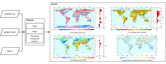
2. Materials and Methods

2.1. Data and Processing

2.1.1. LST

LST data were collected by the MODIS sensor, a key instrument of the Terra and Aqua satellites. The LST products were extracted from the MOD11C3 collection 6 dataset from 1 January 2001 to 31 December 2016, which provided monthly composited and averaged LST at a 0.05° spatial resolution (5.6 km × 5.6 km at the Equator), and obtained from Earthdata Search (https://search.earthdata.nasa.gov/). There are 17 scientific data sets (SDS) in this product. The band named LST_Day_CMG was extracted as day time LST to analyze the variation of LST. The standard deviation of the MODIS V006 LST errors were within 1 K [53]. The mean value composite (MVC) method was used to calculate annual average values of LST in the period of 2001–2016.

2.1.2. NDVI

The Terra MODIS NDVI products were extracted from MOD13C2 collection 6 datasets, which were composed of 16-day global composite images from January 2001 to December 2016, and provided by the Earthdata Search, with a spatial resolution at 0.05°. It is derived from the red and near-infrared reflectance ratio as follows [23]:

NDVI = (NIR − R)/(NIR + R)

(1)

where NIR and R are the amounts of near-infrared (the reflectance of band 2 of MODIS) and red light (the reflectance of band 1 of MODIS).

Although the product has eliminated some clouds and bidirectional reflectance of ground objects [54], MODIS NDVI time series data are still influenced by the clouds and atmospheric water vapor. A simple but efficient method, the mean-value iteration filter, was used to reduce the noise and reconstruct a high quality of NDVI time series by using the following equation [55]:

Δ_i = |NDVI_i − (NDVI_i−1 + NDVI_i+1)/2|

(2)

where NDVI_i represents the ith monthly NDVI, with range from 1 to 192 (16 years). A small percentage of the multiyear NDVI average of each pixel was set at a threshold (Δ). The results of several test showed that 10% was the optimal threshold in this study. When Δ_i > Δ, the NDVI_i was replaced by (NDVI_i−1 + NDVI_i+1)/2. The procedure is iterated until all Δ_i are within the given threshold.

The seasonal characteristics of plants can cause substantial differences in vegetation cover between seasons. Thus, the seasonally integrated normalized difference vegetation index (SINDVI), sum of NDVI values exceeding the threshold (commonly defined as NDVI > 0.1) [56,57,58], was used to monitor the interannual change of vegetation. It can identify vegetation distribution and growth state simultaneously. Due to the large influence of intermittent climatic factors such as precipitation on vegetation growth, compared with NDVI, SINDVI could better describe the interannual variation [59].

2.1.3. PM_2.5

PM_2.5 data were significantly consistent (R² = 0.81) with the monitoring results of PM_2.5 concentrations [60] obtained from the Atmospheric Composition Analysis Group (http://fizz.phys.dal.ca/~atmos/martin/) with a spatial resolution of 0.1°. To match the resolutions of the LST and SINDVI datasets, the data were resampled to 0.05° latitude × 0.05° longitude using the nearest neighbor method. The unit for these data was μg/m³. These data only included the region spanning from 69.8°N to 54.8°S and 180°E to 180°W. The objective of this study was to detect global change trends and impact of PM_2.5 on LST. Because of lower PM_2.5 concentrations in the Arctic and Antarctica, these data could meet the target of this study.

2.2. Methodology

2.2.1. Inter-Annual Variation Analysis

To determine the spatiotemporal differences, the annual change tendency was quantified at a global scale. Monthly time series data were processed to form yearly time series data; in this way, for each pixel the time series has a length of 16, spanning from 2001 to 2016, and the number of pixels in each band are 3600 × 7200. Linear regression and ordinary least squares methods were used to estimate the rate and range of changes at regional and global scales [9,57,61,62]. Random noises within 1K were added to LST data to test the sensitivity of constant biases. It was worth nothing that the slope and range were not affected by possible constant biases present in the data. Therefore, the slope and range were used to assess the interannual variations in LST, SINDVI, and PM_2.5. The slope represents the change rate of each pixel from 2001 to 2016 calculated by the ordinary least-squares estimation via linear regression as follows:

$$slope=\frac{n\times {\sum }_{i=1}^n\left(i\times A_i\right)-{\sum }_{i=1}^{n}i\times {\sum }_{i=1}^n{A}_i}{n\times {\sum }_{i=1}^n{i}^2-{\left({\sum }_{i=1}^{n}i\right)}^2}$$

(3)

where n represents the length of the time series (in this research, n = 16); A_i represents the ith year for SINDVI, PM_2.5 or the average LST; and the value of i ranges from 1 to n.

The range can evaluate the magnitude of change. Each pixel value represents the total variation during the period of 2001–2016.

$$range=slope\times \left(n-1\right)$$

(4)

where n is similar to the definition of slope and represents the length of the time series.

If slope > 0, it means that there is an increasing trend during the past 16 years, whereas the opposite means that it is decreasing. A large absolute value indicates a dramatic change, while the absolute value close to 0 indicates little variation.

2.2.2. Correlation Analysis

For clear descriptions of the relationships between LST with SINDVI and PM_2.5, Pearson’s correlation coefficients (r) was used to indicate the correlation. It was conducted as follows:

$$r_{xy}=\frac{{\sum }_{i=1}^n\left(x_i-\overline{x}\right)\left(y_i-\overline{y}\right)}{\sqrt{{\sum }_{i=1}^n{\left(x_i-\overline{x}\right)}^2}\sqrt{{\sum }_{i=1}^n{(y_i-\overline{y})}^2}}$$

(5)

where x_i and y_i represent LST and either SINDVI or PM_2.5 in the ith year, respectively; and $\overline{x}$ and $\overline{y}$ represent the corresponding averages over 16 years.

At the same time, partial correlations were conducted to assess the dominant factor of each pixel. The partial correlation analysis refers to the process of removing the influence of the third variable when two variables are related to the third variable at the same time, and it only analyzes the correlation between the other two variables [56]. When the degree of correlation between LST and SINDVI was estimated, the influence of PM_2.5 could be removed. The partial correlation coefficient was calculated as follows:

$$r_{xy\left(z\right)}=\frac{r_{xy}-r_{xz}{r}_{yz}}{\sqrt{\left(1-r_{xz}^2\right)\left(1-r_{yz}^2\right)}}$$

(6)

where r_xy(z) is the partial correlation coefficient, representing the degree of correlation between x and y without z; and r_xy, r_xz and r_yz are simple correlation coefficients.

The C program was used to calculate the average LST for each year from 192 scene images, reconstruct the NDVI, summarize the NDVI during growing season in order to obtain the annual SINDVI and analyze the correlation. The Mollweide projection, an equal-area pseudo-cylindrical map projection, was used to count regional areas.

3. Results

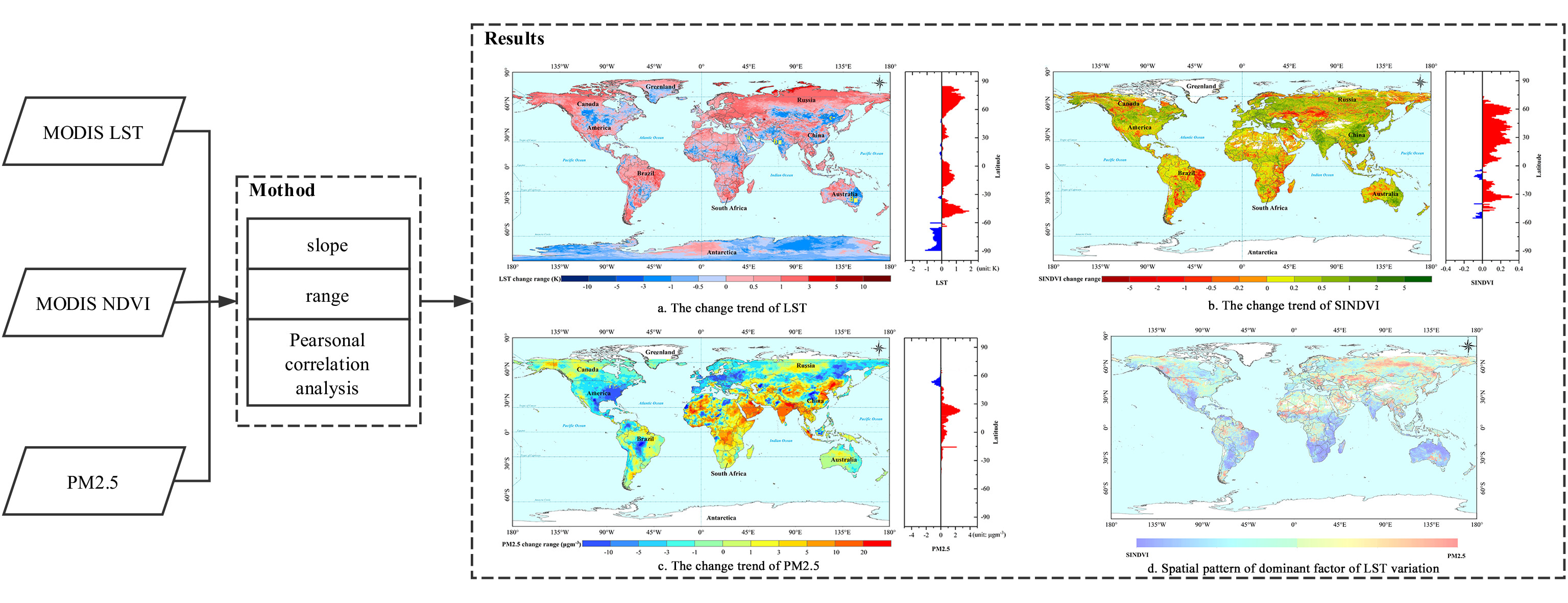
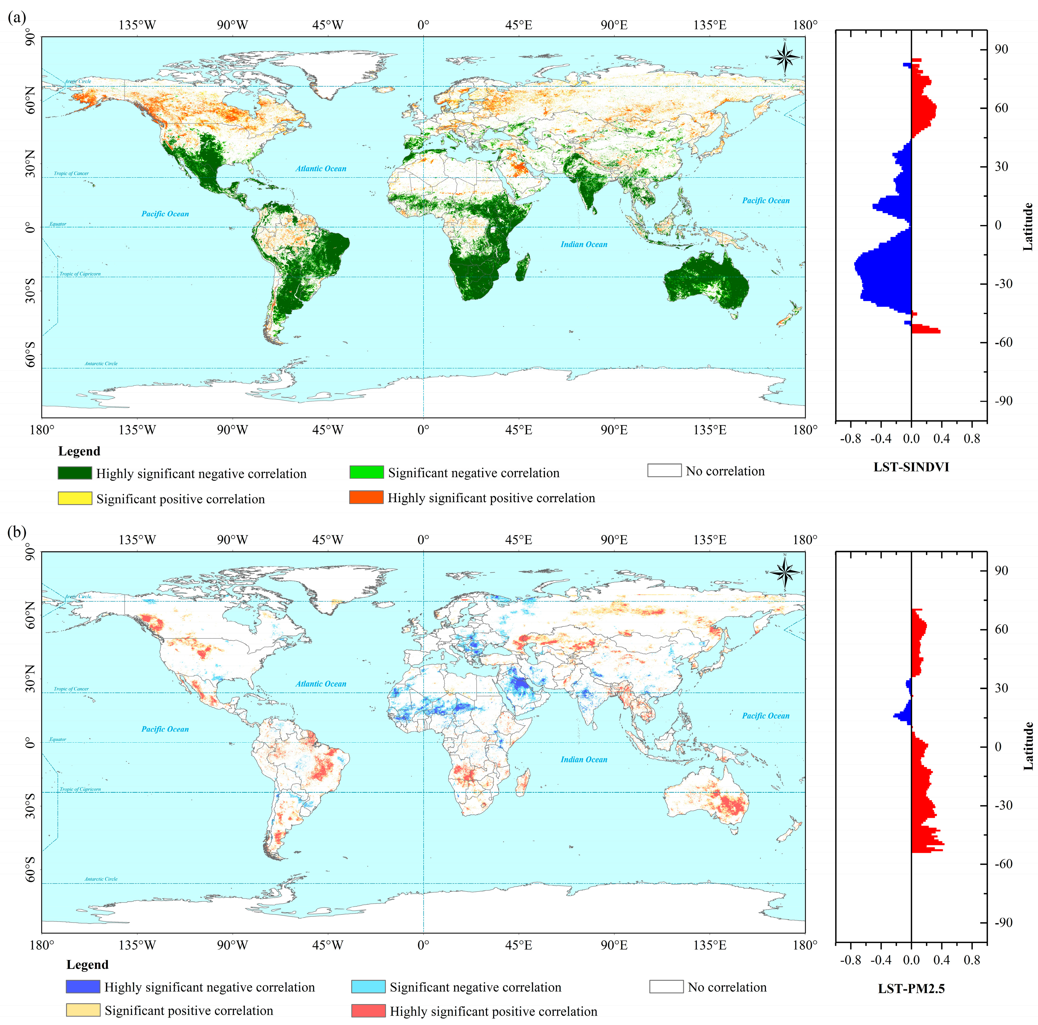
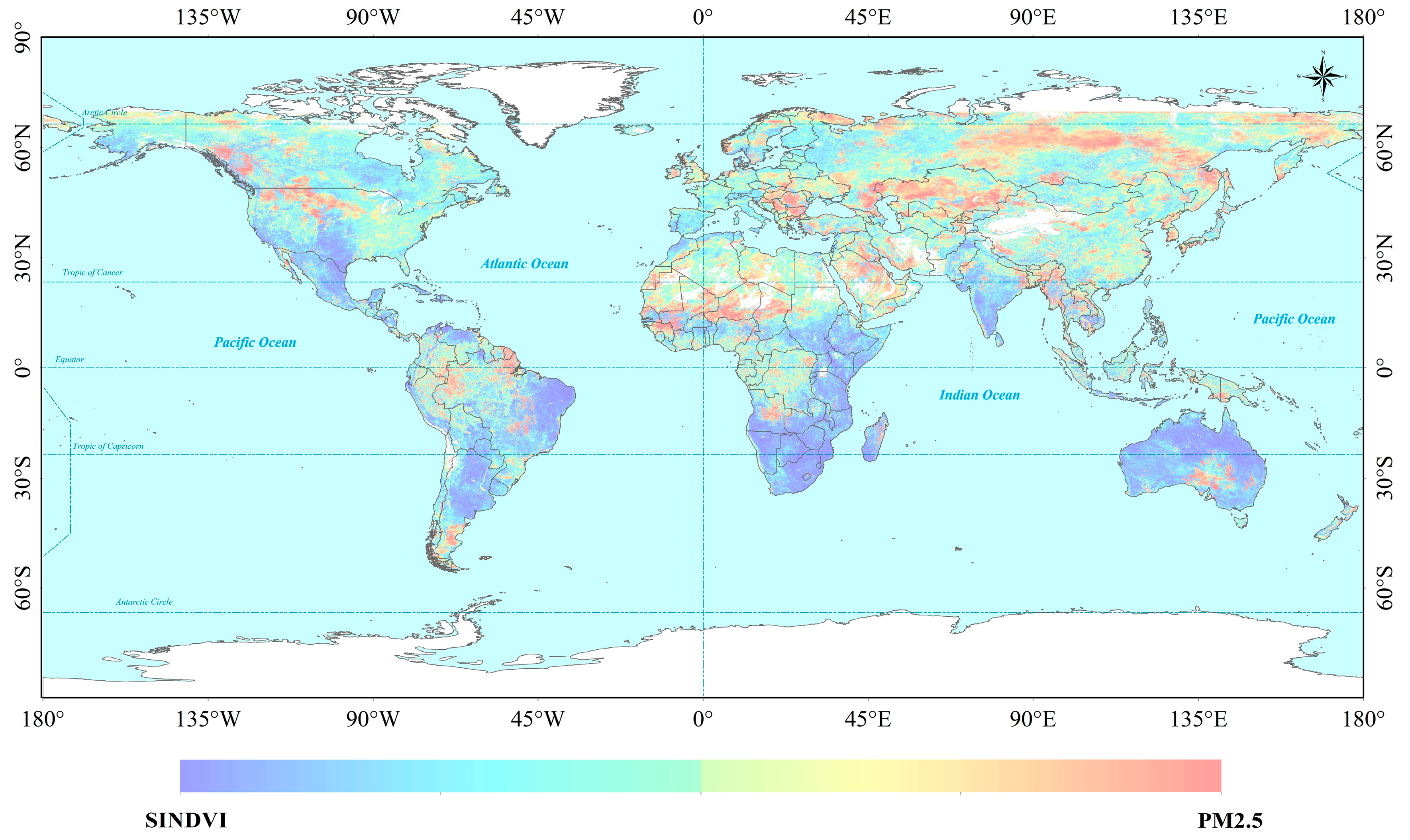
3.1. Spatiotemporal Changes in LST, SINDVI, and PM_2.5 Concentrations

The global land surface temperature presented an increasing trend, with a global mean rise of 0.17 K from 2001 to 2016 (

Table 1. Changes of LST, SINDVI, and PM_2.5 at different latitudinal bands from 2001 to 2016.

	Global	60°–90°N	30°–60°N	0°–30°N	0°–30°S	30°–60°S	60°–90°S
LST	0.17	1.10	0.23	0.07	0.47	0.31	−0.56
SINDVI	0.04	0.03	0.12	0.05	0.01	0.01	0.00
PM2.5	1.02	−0.20	−0.19	4.03	1.20	0.47	--

). LST increased at various degrees across 62.4% of the land area, with the exception in some regions such as the Antarctic, central North America, Central Asia, and eastern Australia (Figure 1a). An LST increase of 15 K was found in the Aral Sea, where water level decreased by 23 m, surface area decreased by 74%, and lake volume decreased by 90% [63], experiencing extreme desiccation [62]. The temperature of most regions increased within the range between 0 and 3 K, which accounts for 61.9% of the global land area. The Arctic experienced a marked warming trend, especially in northern Russia; however, the Antarctic, an area of approximately 14 million km², showed a cooling trend. In the mid-latitudes of the Northern Hemisphere, such as southeast Canada, northern United States, eastern Kazakhstan, Mongolia, and Northeast China, dramatic decreases in LST were detected.

Variable solar radiation causes different climate zones and LST along the latitude. As shown in Figure 1a and Table 1, LST had an increasing trend, except for the areas at high latitudes in the Southern Hemisphere. In the high latitudes of the Northern Hemisphere, the change range increased firstly before a sharp decline. LST increased by an average of 0.30 K in the mid-latitudes of northern hemisphere, and it fluctuated slightly in the low-latitude areas. Compared with the Northern Hemisphere, there were two distinct peaks both at low- and mid-latitudes, and the larger one was an increase of 1.85 K at 48°S.

SINDVI presented a greening trend all over the world [57], with an average value of 0.04 during the period of 2000–2016. Approximately 58.4% of the global area showed an increasing trend. Arctic, Antarctic, and high mountains were coved by snow for most time of the year. Approximately 9.8% of the global land was covered with snow all the year round, and SINDVI had no change in these regions. About 31.8% of other areas experienced a downward trend. Approximately 54.5% of the area’s increase range of SINDVI was between 0 and 1, and 40.5% ranged from −1 to 0. The vegetation cover in central and southeastern China, northwestern India, and eastern Australia increased markedly. In addition, an increase appeared in Europe and most parts of North America. However, the SINDVI decreased significantly in eastern Brazil, northern Argentina, northern Kazakhstan, southeastern Africa, and western Australia.

The latitudinal SINDVI varied from −0.11 to 0.33, with an obvious increasing trend in the Northern Hemisphere, which indicated the great increase in the vegetation coverage in the Northern Hemisphere (Figure 1b and Table 1). SINDVI in Southern Hemisphere (between 15°S to 30°S) also increased, with fluctuation within ±0.15. However, a dramatic decrease (from 0.32 to −0.09) was found between 34°S and 40°S, and there were more rapidly latitudinal fluctuations between 40°S and 55°S.

PM_2.5 concentrations also had an increasing trend (1.02 μg/m³). The global distribution of PM_2.5 was shown in Figure 1c. The air quality in America, Europe, and eastern Russia improved greatly. PM_2.5 concentrations in Africa as a whole showed an increasing trend, and most regions had increased by 10 μg/m³. PM_2.5 in Asia, such as Saudi Arabia, India, and China, increased noticeably, indicating serious air pollution. Slight fluctuations were found in Australia.

In the Northern Hemisphere, PM_2.5 concentrations decreased at mid-latitudes, but increased markedly at low latitudes. In the Southern Hemisphere near the tropics, the concentrations of PM_2.5 increased slightly.

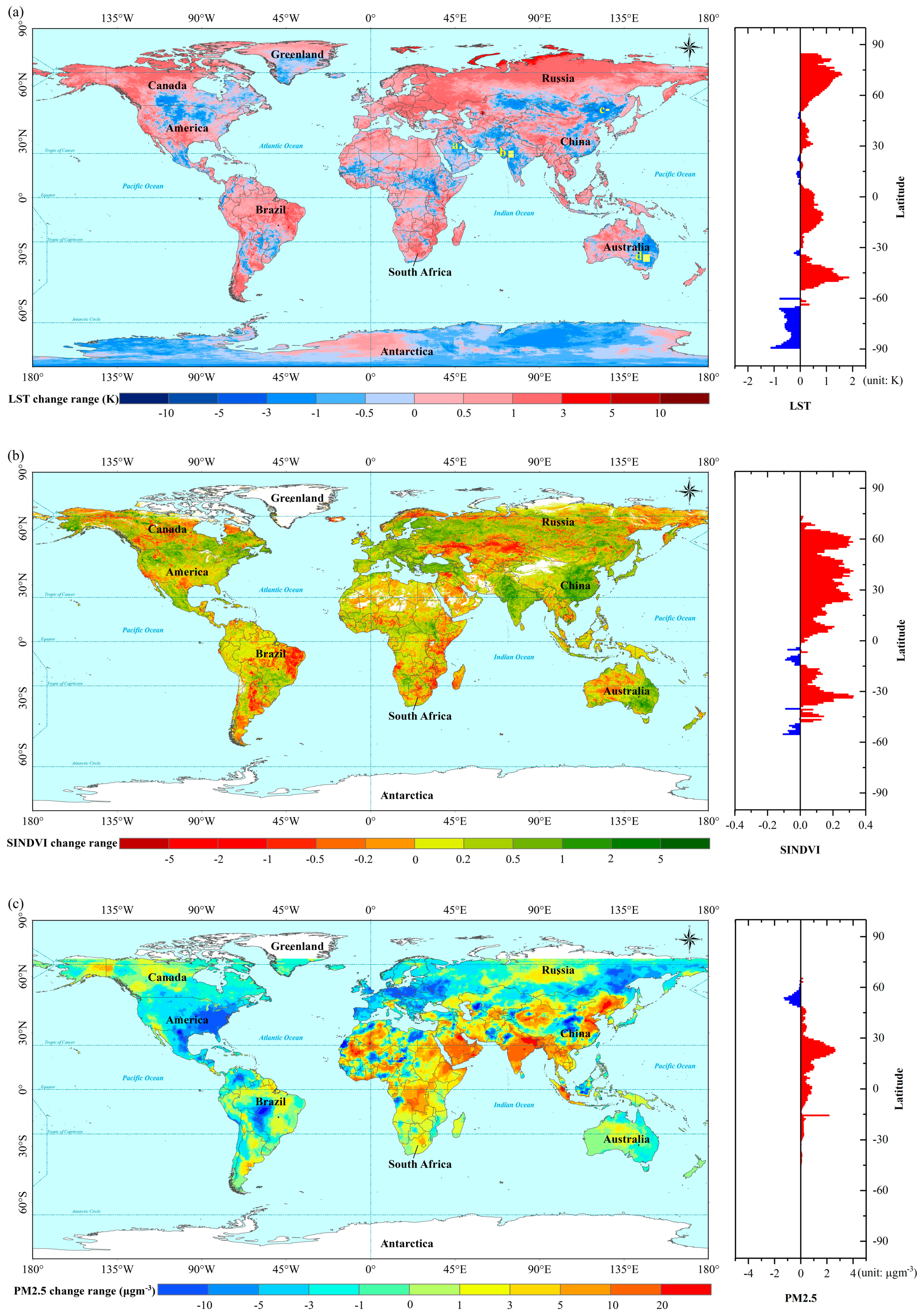
3.2. Correlation Analysis

The Pearson correlation coefficients were calculated based on each pixel, as shown in Figure 2 (left). The results indicated a significant positive correlation between the LST and SINDVI in most areas of the Northern Hemisphere. In contrast, a highly significant negative correlation appeared in most areas of the Southern Hemisphere, especially Brazilian plateau, Pampas steppe, southeastern Africa, and Australia.

Latitudinal patterns of Pearson correlation were shown in Figure 2 (right). In the Northern Hemisphere, a positive correlation between LST and SINDVI was found at high latitudes, but a negative correlation was found in other latitudinal zones. In the Southern Hemisphere, the correlation between LST and SINDVI increased then decreased along with a rising latitude. Strong negative correlations between LST and SINDVI occurred at 15–35°S (i.e., mid-to-low latitudes in the Southern Hemisphere), and the negative correlation gradually weakened from latitude of 40°S.

Except for low latitudes in the Northern Hemisphere, a positive correlation between LST and PM_2.5 appeared around the world. Compared with regions in north of the equator, those in south of the equator had stronger positive correlations. Positive correlations between LST and PM_2.5 existed in central Eurasia, South America, and eastern Australia, where PM_2.5 fluctuated slightly. The negative correlations between LST and PM_2.5 were mainly concentrated in Europe, West Asia, and south of Sahara Desert. In these areas, PM_2.5 experienced dramatic changes, increasing in West Asia especially in Saudi Arabia and decreasing in Europe such as Poland, Germany, and Romania. Therefore, the effect of PM_2.5 on LST was complex, and it was related to the changes of PM_2.5 concentrations. A small amplitude increasing of PM_2.5 concentration increased LST due to the heat retention effect of PM_2.5 on global surfaces, with a result of a positive correlation. However, a marked increase in PM_2.5 concentration prevented solar radiation from reaching the surface, reducing surface energy and causing a decrease in LST.

3.3. Dominant Factor Analysis

The partial correlation coefficients (i.e., r _{LST SINDVI (PM2.5)} and r _{LST PM2.5 (SINDVI)}) were calculated based on pixels to analyze the main factors causing surface temperature changes (Figure 3). If r _{LST SINDVI (PM2.5)} was larger than r _{LST PM2.5 (SINDVI)}, the SINDVI was considered to be the main factor. The opposite result indicated PM_2.5 had a larger effect on LST.

In most parts of the world, SINDVI was found to be the dominant factor (Figure 3). SINDVI increased markedly in the mid-latitude of the Northern Hemisphere, especially over the East European Plain, Labrador Plateau, and India. It decreased obviously in east of the Brazilian Plateau and southeast of Africa. The decrease in vegetation cover caused by human activities led to the increase in LST.

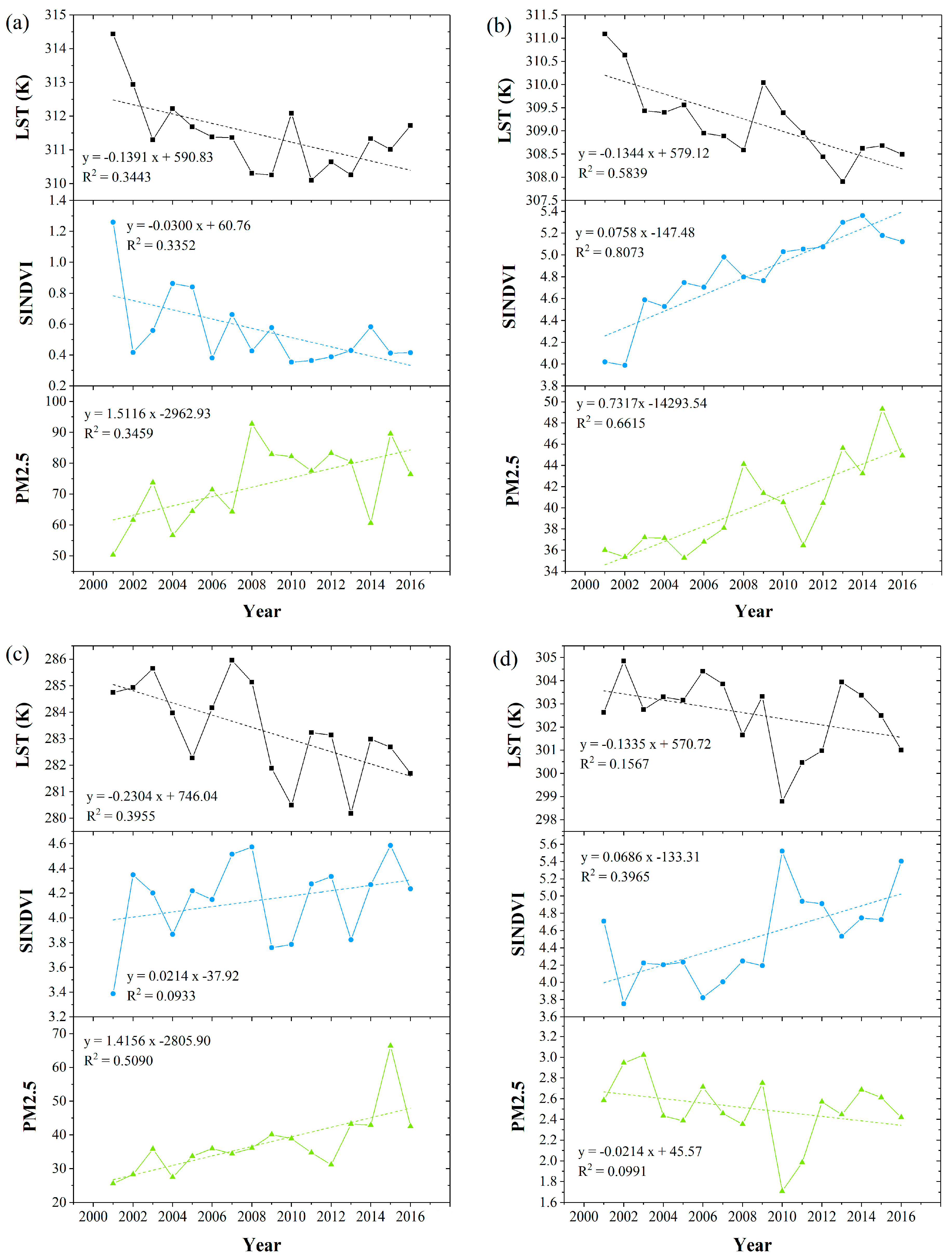
3.4. Significant Decreases in LST on Regions of Interest (ROIs)

Four regions of interest (ROIs) where LST decreased sharply were found in Saudi Arabia (ROI-a), India (ROI-b), Northeast China (ROI-c), and Australia (ROI-d). The spatial positions of ROIs were shown in Figure 1a in yellow and the locations were shown in

Table 2. Locations of four regions of interest (ROIs).

Region Code	Bottom Left Corner	Top Right Corner	Pixel Numbers
ROI-a	25.85°N, 47.30°E	27.30°N, 48.50°E	696
ROI-b	21.30°N, 73.25°E	25.05°N, 76.20°E	4425
ROI-c	46.10°N, 125.20°E	47.30°N, 127.20°E	960
ROI-d	34.15°S, 145.05°E	30.10°S, 148.70°E	5913

.

3.4.1. Saudi Arabia

LST in Saudi Arabia (ROI-a) has decreased by 2.09 K over the past 16 years (Figure 4a). SINDVI in this region also decreased with a slope of −0.03, but PM_2.5 increased dramatically, with a slope of 1.512. The interannual variations in ROI-a were shown in Figure 4a. The correlation analysis showed a significantly positive correlation between LST and SINDVI (r = 0.661, p < 0.01) and a significantly negative correlation between LST and PM_2.5 (r = −0.746, p < 0.01), which means that both SINDVI and PM_2.5 contributed to the changes in LST. However, the partial correlation analyses indicated lower confidence levels (p > 0.05,

Table 3. Statistical analysis of relation between LST with SINDVI and PM_2.5 in the regions of interest (ROIs).

	Simple Correlation Coefficient				Partial Correlation Coefficient
	r LST SINDVI	p	r LST PM2.5	p	r LST SINDVI (PM2.5)	p	r LST PM2.5 (SINDVI)	p
ROI-a	0.661 **	0.005	−0.746 **	0.001	0.249	0.371	−0.511	0.051
ROI-b	−0.877 **	0.000	−0.630 **	0.009	−0.789 **	0.000	−0.106	0.708
ROI-c	0.336	0.203	−0.416	0.109	0.569 *	0.027	−0.608 *	0.016
ROI-d	−0.849 **	0.000	0.743 **	0.001	−0.736 **	0.002	0.513	0.051

* indicates a statistically significant p-value (p < 0.05); **indicates p < 0.01.

). Therefore, the effects of vegetation cover cannot be ignored in this area.

3.4.2. India

LST experienced a marked decrease as SINDVI and PM_2.5 increased in India (Figure 1). The interannual variations in ROI-b were shown in Figure 4b. The variation in vegetation cover played the leading roles in affecting LST changes during the period from 2001 to 2016 (Figure 3). The correlation analysis showed that LSTs were significantly correlated to both SINDVI and PM_2.5, with Pearson correlation coefficients of −0.877 (p < 0.01) and −0.630 (p < 0.01), respectively. However, the partial correlation analysis indicated that the correlation between LST and SINDVI (r _{LST SINDVI (PM2.5)} = −0.789, p < 0.01) was more significant than that between LST and PM_2.5 (r _{LST PM2.5 (SINDVI)} = −0.106).

3.4.3. China

LST showed an increasing trend in West China, but a reverse trend in East China, particularly in Northeast China (Figure 1a). The interannual variations in ROI-c were shown in Figure 4c. Interestingly, the partial correlation analyses indicated a significantly positive correlation between LST and SINDVI and a significantly negative correlation between LST and PM_2.5, while the simple correlation coefficients were smaller than the partial correlation coefficients (Table 3). Therefore, the interaction between SINDVI and PM_2.5 weakened their respective effects on LST in the Northeast China.

3.4.4. Australia

LST in Australia showed a decreasing trend, with a noticeable increase in SINDVI and a slight decrease in PM_2.5 (Figure 1). The interannual variations in ROI-d were shown in Figure 4d. In 2010, the value of LST and PM_2.5 were low, but SINDVI reached its peak (Figure 4d). The simple correlation analysis showed significant relationship between LST with SINDVI and PM_2.5, but the partial correlation analysis indicated that SINDVI had a larger impact on LST than PM_2.5 (Table 3).

4. Discussion

4.1. Potential Causes for Variations in LST, SINDIV, and PM_2.5

LST is very sensitive to the global climate changes. It had a prominent increasing trend in the Arctic, but a decreasing trend over the Antarctic. This is consistent with the conclusion of Overland et al. [64] that the North and South poles experienced opposite climate changes. Authors identified anthropogenic influence as the primary cause for sea ice reduction in the Arctic [65]. Under the background of global warming, researchers have paid more attention to the warming in the Arctic due to the importance of global sea level rise, especially regarding the Greenland ice sheet [66]. LST could also be used to monitor glacial melt zones based on remote sensing technology. LSTs increased in the Arctic, and the surface temperature of North Greenland had risen by approximately 1 K over the past 16 years (Figure 1a). The main indicators of Arctic temperature increase include reducing sea ice and permafrost. In addition, LST could indicate the burn severity of forest fires [67]. The increase in LST (0.073–0.325 K) has deteriorated forest fires in Siberian boreal forests. In addition to direct warming by fires, lower albedo with darker surfaces and lower evapotranspiration due to biomass burning can increase energy absorption by land surface and decrease the evaporative cooling, with the consequence of higher LST [68].

Although both the Arctic and Antarctic were subjected to similar solar radiation and increasing greenhouse gas concentrations, the two regions had undergone different variations [64]. Studies showed that decreasing LSTs in the Antarctic may be related to the ozone hole [69]. Turner et al. [70] suggested that the ozone hole would shield global warming in the Antarctic. Ozone depletion in the stratosphere had intensified polar vortices, and winds over the center of the Antarctic continent had strengthened the change of weather patterns over the mainland. Strong winds have effectively separated the Antarctic from global warming, with a result of a decrease in LST and an increase in snowfall [71].

SINDVI value was used to denote interannual variations of vegetation productivity [58]. It integrated NDVI over the growth season and weaken the details of NDVI variation. Vegetation cover measured by SINDVI showed a greening trend at the global scale from 2001 to 2016 (Figure 1b). Specifically, vegetation greening trends increased in midlatitude areas of the Northern Hemisphere. Other studies demonstrated that snow cover decreased dramatically in those regions [57]. As a result of global warming, the melting of snow and ice produced a large amount of water that could be used for irrigating plant. In addition, longer growing season caused by more heat can also led to the increases in SINDVI. A dramatic browning trend was found in central Asia (Figure 1b). In this area, a warming climate in the summer worsened the aridity [72]. The decreases in precipitation and aridity were the main reasons for the decreases in SINDVI [72].

The sources of air pollutants were diversified, such as biomass burning, fossil fuel combustion, and industrialization [73,74]. PM_2.5 in the atmosphere could be emitted directly by combustion or mechanical processes and it can also be generated by chemical reactions of inorganic or organic molecules in the atmosphere [73]. The time series analyses of the interannual mean PM_2.5 concentration demonstrated an increasing trend at a global scale (Figure 1c and Table 1). Dramatic decreases in PM_2.5 were observed in the Eastern USA and Europe because of effective pollution control measures, but an opposite trend was found in Sub-Saharan Africa due to biomass burning and higher concentration of mineral dust [60]. New research showed that the emissions of sulfur dioxide had increased by 50% in India from 2007 to 2017 [75]. The sharp increase in PM_2.5 in India was influenced by both anthropogenic and natural factors such as chemical processes [73,75] and mineral dust [60]. The regions where PM_2.5 was the dominate factor for the change in LST were mainly distributed in central Russia and Kazakhstan where the concentration of PM_2.5 increased because of the biomass burning [76], and Saudi Arabia where a lot of mineral dust contributed to the increase in PM_2.5.

4.2. Influence of SINDVI and PM_2.5 on LST

This study analyzed the effects of the vegetation cover measured by SINDVI and air pollution measured by PM_2.5 on the variation in LST. Previous studies showed the lower LSTs with higher vegetation cover [18,77]. Similarly, the current study found a significant negative relationship between SINDVI and LST in the Southern Hemisphere and low latitude areas of the Northern Hemisphere. On the contrary, a positive relationship between LST and SINDVI was found in high latitude areas. Different from the low latitude of Northern Hemisphere, high latitude areas are characterized by lesser solar radiation and lower temperature. Plant photosynthesis is limited particularly by lower temperature and increase in temperature including LST will promote plant growth and NDVI values in high latitude. Therefore, a positive relationship between LST and SINDVI was found in high latitude. A study found that although most regions experienced overall greenness, the increase rate decreased and browning trend expanded in the Northern Hemisphere especially in northern mid-low latitudes [26]. It could be the reason for that the negative relationship between SINDVI and LST in the Northern Hemisphere was weaker than that in the Southern Hemisphere (Figure 3). Furthermore, compared with past time, the increasing temperature caused a longer plant growth season. It partially caused the increase in SINDVI [78]. Therefore, the browning trend was hidden in the greenness in the Northern Hemisphere. In addition, drought can cause higher LST, but the legacies of drought were different among forest, shrubs, and grass in the North Hemisphere [79].

SUHI and the air pollution have become two major problems along with urbanization without proper environmental protection [43]. The positive correlation between LST and PM_2.5 was found in most areas from 2001 to 2016 (Figure 2b). However, negative correlation was also identified in Saudi Arabia, northeast China and south of Sahara Desert. It might be caused by a different rate of the variation in PM_2.5 concentrations. Cooling effect of aerosol was found in the urban areas [44]. Radiative effects of aerosols, reducing solar shortwave radiation and increasing atmospheric longwave radiation, have a marked cooling effect on air temperature, especially downwind of the city cluster [42]. The cooling effects of aerosol can explain the negative relation between LST and PM_2.5 in Saudi Arabia, northeast China and south of Sahara Desert where PM_2.5 increased markedly. The increase of PM_2.5 can reduce solar radiation reaching land by scattering more radiation back to space, but it could also reduce the surface longwave flux and latent heat flux which may increase LST [80,81].

In addition, Hajiloo et al. [37] used a geographically weighted regression model to assess the relationship between environmental parameters and PM_2.5 concentrations. They found a negative correlation between LST with PM_2.5 in western Tehran and a positive correlation in eastern Tehran which resulted from asymmetry distribution of vegetation. However, different trends of SINDVI did not cause opposite correlation in ROI-a and ROI-b (Figure 4a,b). Therefore, other factors may play a more important part in the negative correlation between LST and PM_2.5 in the two areas.

4.3. Limitations and Future Research

Same as many studies, there are limitations in the current research. Due to the spatial heterogeneity, LST can be affected by many factors, such as elevation, albedo, meteorological parameters, human activities, and others. [9,18,57,82]. However, because of the limitation of high spatial resolution remote sensing images and statistical data at a global scale, other factors rather than SINDVI and PM_2.5 have not yet been considered in this study. In addition, the enhanced vegetation index (EVI) was more sensitive than NDVI in some regions, such as tropical rainforests with high biomass [83]. The saturation of NDVI might underestimate the correlation between LST and vegetation cover. In future studies, other vegetation indexes can be used to analyze vegetation changes in the regions with saturation of NDVI. In addition, it is important to develop models including more climatic, topographical, and socio-economic factors such as precipitation, wind speed, elevation, SUHI, population, and others for better estimate the changes of LST.

5. Conclusions

In this study, the spatiotemporal trends of global land surface temperature, vegetation cover, and air quality were analyzed during the period of 2001–2016. The research evaluated the influence of vegetation cover and PM_2.5 on land surface temperature. A total of 62.4% of the world’s land surface temperature exhibited a increasing trend from 2001 to 2016. A total of 58.2% of regions had an increasing trend of SINDVI, indicating that vegetation coverage increased from a global aspect. The concentrations of PM_2.5 showed an increasing pattern mainly in developing countries, for example China and India, and a decreasing pattern mostly in developed countries, such as the USA. A significant negative correlation between vegetation and land surface temperature indicated vegetation was the main driver for land surface temperature changes in most areas on the earth. The effect of PM_2.5 on surface temperature was not uniform. A significant increase in PM_2.5 concentrations caused a decrease in surface temperature, but a slight increase in PM_2.5 concentrations increased surface temperature. In future studies, models including more parameters should be developed to more accurately analyze the variation in land surface temperature.

References

1. Estrada, F.; Martins, L.F.; Perron, P. Characterizing and attributing the warming trend in sea and land surface temperatures. Atmósfera 2017, 30, 163–187. [Google Scholar] [CrossRef] [Green Version]
2. Qin, D.; Thomas, S.; TSU (Bern & Beijing). Highlights of the IPCC working group|fifth assessment report. Clim. Chang. R 2014, 10, 1–6. [Google Scholar]
3. Ji, F.; Wu, Z.; Huang, J.; Chassignet, E.P. Evolution of land surface air temperature trend. Nat. Clim. Chang. 2014, 4, 462–466. [Google Scholar] [CrossRef]
4. Sun, L.; Sun, R.; Li, X.; Chen, H.; Zhang, X. Estimating evapotranspiration using improved fractinal vegetation cover and land surface temperatur space. J. Resour. Ecol. 2011, 2, 225–231. [Google Scholar]
5. Bechtel, B. A new global climatology of annual land surface temperature. Remote Sens. 2015, 7, 2850–2870. [Google Scholar] [CrossRef]
6. Kerr, Y.H.; Lagouarde, J.P.; Nerry, F.; Ottlé, C.; Quattrochi, D.A.; Luvall, J.C. Land surface temperature retrieval techniques and applications. Therm. Remote Sens. LSP 2000, 33–109. [Google Scholar] [CrossRef]
7. Li, Z.; Tang, B.; Wu, H.; Ren, H.; Yan, G.; Wan, Z.; Trigo, I.F.; Sobrino, J.A. Satellite-derived land surface temperature: Current status and perspectives. Remote Sens. Environ. 2013, 131, 14–37. [Google Scholar] [CrossRef] [Green Version]
8. Song, L.; Liu, S.; Kustas, W.P.; Nieto, H.; Sun, L.; Xu, Z.; Skaggs, T.H.; Yang, Y.; Ma, M.; Xu, T.; et al. Monitoring and validating spatially and temporally continuous daily evaporation and transpiration at river basin scale. Remote Sens. Environ. 2018, 219, 72–88. [Google Scholar] [CrossRef]
9. Peng, J.; Ma, J.; Liu, Q.; Liu, Y.; Hu, Y.N.; Li, Y.; Yue, Y. Spatial-temporal change of land surface temperature across 285 cities in China: An urban-rural contrast perspective. Sci. Total Environ. 2018, 635, 487–497. [Google Scholar] [CrossRef]
10. Zhao, L.; Yang, Z.-L.; Hoar, T.J. Global soil moisture estimation by assimilating AMSR-E brightness temperatures in a coupled CLM4–RTM–DART system. J. Hydrometeorol. 2016, 17, 2431–2454. [Google Scholar] [CrossRef]
11. Anastasios, P.; Theleia, M.; Constantinos, C. Quantifying the trends in land surface temperature and surface urban heat island intensity in mediterranean cities in view of smart urbanization. Urban Sci. 2018, 2, 16. [Google Scholar] [CrossRef]
12. Wan, Z.; Jeff, D. A generalized split-window algorithm for retrieving land-surface temperature from space. IEEE Trans. Geosci. Remote Sens. 1996, 34, 892–905. [Google Scholar]
13. Masiello, G.; Serio, C.; De Feis, I.; Amoroso, M.; Venafra, S.; Trigo, I.F.; Watts, P. Kalman filter physical retrieval of surface emissivity and temperature from geostationary infrared radiances. Atmos. Meas. Tech. 2013, 6, 3613–3634. [Google Scholar] [CrossRef] [Green Version]
14. Yu, W.; Ma, M.; Li, Z.; Tan, J.; Wu, A. New Scheme for validating remote-sensing land surface temperature products with station observations. Remote Sens. 2017, 9, 1210. [Google Scholar] [CrossRef]
15. Masiello, G.; Serio, C.; Venafra, S.; Liuzzi, G.; Göttsche, F.; Trigo, I.F.; Watts, P. Kalman filter physical retrieval of surface emissivity and temperature from SEVIRI infrared channels: A validation and intercomparison study. Atmos. Meas. Tech. 2015, 8, 2981–2997. [Google Scholar] [CrossRef]
16. Masiello, G.; Serio, C.; Venafra, S.; Liuzzi, G.; Poutier, L.; Göttsche, F.-M. Physical retrieval of land surface emissivity spectra from hyper-spectral infrared observations and validation with in situ measurements. Remote Sens. 2018, 10, 976. [Google Scholar] [CrossRef]
17. Ghent, D.; Good, E.; Bulgin, C.; Remedios, J.J. A spatio-temporal analysis of the relationship between near-surface air temperature and satellite land surface temperatures using 17 years of data from the ATSR series. J. Geophys. Res. Atmos. 2017, 122, 9185–9210. [Google Scholar]
18. Deng, Y.; Wang, S.; Bai, X.; Tian, Y.; Wu, L.; Xiao, J.; Chen, F.; Qian, Q. Relationship among land surface temperature and LUCC, NDVI in typical karst area. Sci. Rep. 2018, 8, 641. [Google Scholar] [CrossRef] [PubMed] [Green Version]
19. Xu, Y.; Shen, Y.; Wu, Z. Spatial and temporal variations of land surface temperature over the Tibetan Plateau Based on Harmonic analysis. Mt. Res. Dev. 2013, 33, 85–94. [Google Scholar] [CrossRef]
20. Carlson, T.N.; Gillies, R.R.; Perry, E.M. A method to make use of thermal infrared temperature and NDVI measurements to infer surface soil water content and fractional vegetation cover. Remote Sens. 1994, 9, 161–173. [Google Scholar] [CrossRef]
21. Vlassova, L.; Pérez-Cabello, F.; Mimbrero, M.; Llovería, R.; García-Martín, A. Analysis of the relationship between land surface temperature and wildfire severity in a series of Landsat images. Remote Sens. 2014, 6, 6136–6162. [Google Scholar] [CrossRef]
22. Van Nguyen, O.; Kawamura, K.; Trong, D.P.; Gong, Z.; Suwandana, E. Temporal change and its spatial variety on land surface temperature and land use changes in the Red River Delta, Vietnam, using MODIS time-series imagery. Environ. Monit. Assess. 2015, 187, 464. [Google Scholar] [CrossRef] [PubMed]
23. Pettorelli, N.; Vik, J.O.; Mysterud, A.; Gaillard, J.M.; Tucker, C.J.; Stenseth, N.C. Using the satellite-derived NDVI to assess ecological responses to environmental change. Trends Ecol. Evol. 2005, 20, 503–510. [Google Scholar] [CrossRef] [PubMed]
24. Swain, S.; Wardlow, B.D.; Narumalani, S.; Tadesse, T.; Callahan, K. Assessment of vegetation response to drought in Nebraska using Terra-MODIS land surface temperature and normalized difference vegetation index. GISci. Remote Sens. 2013, 48, 432–455. [Google Scholar] [CrossRef]
25. Jingyong, Z.; Wenjie, D.; Congbin, F.; Lingyun, W. The influence of vegetation cover on summer precipitation in China: A statistical analysis of NDVI and climate data. Adv. Atmos. Sci. 2003, 20, 1002–1006. [Google Scholar] [CrossRef]
26. Pan, N.; Feng, X.; Fu, B.; Wang, S.; Ji, F.; Pan, S. Increasing global vegetation browning hidden in overall vegetation greening: Insights from time-varying trends. Remote Sens. Environ. 2018, 214, 59–72. [Google Scholar] [CrossRef]
27. Tan, Z.; Tao, H.; Jiang, J.; Zhang, Q. Influences of climate extremes on NDVI (Normalized Difference Vegetation Index) in the Poyang Lake Basin, China. Wetlands 2015, 35, 1033–1042. [Google Scholar] [CrossRef]
28. Tourre, Y.M.; Jarlan, L.; Lacaux, J.P.; Rotela, C.H.; Lafaye, M. Spatio-temporal variability of NDVI–precipitation over southernmost South America: Possible linkages between climate signals and epidemics. Environ. Res. Lett. 2008, 3, 1–9. [Google Scholar] [CrossRef]
29. Zhang, Y.; Gao, J.; Liu, L.; Wang, Z.; Ding, M.; Yang, X. NDVI-based vegetation changes and their responses to climate change from 1982 to 2011: A case study in the Koshi River Basin in the middle Himalayas. Glob. Planet. Chang. 2013, 108, 139–148. [Google Scholar] [CrossRef]
30. Fathizad, H.; Tazeh, M.; Kalantari, S.; Shojaei, S. The investigation of spatiotemporal variations of land surface temperature based on land use changes using NDVI in southwest of Iran. J. Afr. Earth Sci. 2017, 134, 249–256. [Google Scholar] [CrossRef]
31. Julien, Y.; Sobrino, J.A.; Verhoef, W. Changes in land surface temperatures and NDVI values over Europe between 1982 and 1999. Remote Sens. Environ. 2006, 103, 43–55. [Google Scholar] [CrossRef]
32. Sun, D.; Kafatos, M. Note on the NDVI-LST relationship and the use of temperature-related drought indices over North America. Geophys. Res. Lett. 2007, 34, 1111–1117. [Google Scholar] [CrossRef]
33. Wang, X.; Piao, S.; Ciais, P.; Li, J.; Friedlingstein, P.; Koven, C.; Chen, A. Spring temperature change and its implication in the change of vegetation growth in North America from 1982 to 2006. Proc. Natl. Acad. Sci. USA 2011, 108, 1240–1245. [Google Scholar] [CrossRef] [Green Version]
34. Zhao, S.; Cong, D.; He, K.; Yang, H.; Qin, Z. Spatial-temporal variation of drought in China from 1982 to 2010 based on a modified Temperature Vegetation Drought Index (mTVDI). Sci. Rep. 2017, 7, 17473. [Google Scholar] [CrossRef] [PubMed]
35. Fan, J.; Li, S.; Fan, C.; Bai, Z.; Yang, K. The impact of PM2.5 on asthma emergency department visits: A systematic review and meta-analysis. Environ. Sci. Pollut. Res. 2016, 23, 843–850. [Google Scholar] [CrossRef] [PubMed]
36. Lin, Y.; Zou, J.; Yang, W.; Li, C.Q. A review of recent advances in research on PM2.5 in China. Int. J. Environ. Res. Public Health 2018, 15, 438. [Google Scholar] [CrossRef] [PubMed]
37. Hajiloo, F.; Hamzeh, S.; Gheysari, M. Impact assessment of meteorological and environmental parameters on PM2.5 concentrations using remote sensing data and GWR analysis (case study of Tehran). Environ. Sci. Pollut. Res. Int. 2018, 3, 1–15. [Google Scholar] [CrossRef]
38. Chan, C.K.; Yao, X. Air pollution in mega cities in China. Atmos. Environ. 2008, 42, 1–42. [Google Scholar] [CrossRef]
39. Li, J.; Huang, X.; Yang, H.; Chuai, X.; Wu, C. Convergence of carbon intensity in the Yangtze River Delta, China. Habitat Int. 2017, 60, 58–68. [Google Scholar] [CrossRef]
40. Kampa, M.; Castanas, E. Human health effects of air pollution. Environ. Pollut. 2008, 151, 362–367. [Google Scholar] [CrossRef]
41. Rizwan, A.M.; Dennis, L.Y.C.; Liu, C. A review on the generation, determination and mitigation of Urban Heat Island. J. Environ. Sci. 2008, 20, 120–128. [Google Scholar] [CrossRef]
42. Zhong, S.; Qian, Y.; Zhao, C.; Leung, R.; Wang, H.; Yang, B.; Fan, J.; Yan, H.; Yang, X.-Q.; Liu, D. Urbanization-induced urban heat island and aerosol effects on climate extremes in the Yangtze River Delta region of China. Atmos. Chem. Phys. 2017, 17, 5439–5457. [Google Scholar] [CrossRef] [Green Version]
43. Li, H.; Meier, F.; Lee, X.; Chakraborty, T.; Liu, J.; Schaap, M.; Sodoudi, S. Interaction between urban heat island and urban pollution island during summer in Berlin. Sci. Total Environ. 2018, 636, 818–828. [Google Scholar] [CrossRef] [PubMed]
44. Jin, M.; Shepherd, J.M.; Zheng, W. Urban surface temperature reduction via the urban aerosol direct effect: A remote sensing and WRF model sensitivity study. Adv. Meteorol. 2010, 2010, 681587. [Google Scholar] [CrossRef]
45. Bauer, S.E.; Menon, S. Aerosol direct, indirect, semidirect, and surface albedo effects from sector contributions based on the IPCC AR5 emissions for preindustrial and present-day conditions. J. Geophys. Res. Atmos. 2012, 117, 1–15. [Google Scholar] [CrossRef]
46. Qian, Y.; Kaiser, D.P.; Leung, L.R.; Xu, M. More frequent cloud-free sky and less surface solar radiation in China from 1955 to 2000. Geophys. Res. Lett. 2006, 33, 1–4. [Google Scholar] [CrossRef]
47. Jin, M.S.; Kessomkiat, W.; Pereira, G. Satellite-observed urbanization characters in Shanghai, China: Aerosols, urban heat island effect, and land–atmosphere interactions. Remote Sens. 2011, 3, 83–99. [Google Scholar] [CrossRef]
48. Cao, C.; Lee, X.; Liu, S.; Schultz, N.; Xiao, W.; Zhang, M.; Zhao, L. Urban heat islands in China enhanced by haze pollution. Nat. Commun. 2016, 7, 12509. [Google Scholar] [CrossRef] [Green Version]
49. Ma, M.; Che, T.; Li, X.; Xiao, Q.; Zhao, K.; Xin, X. A Prototype network for remote sensing validation in China. Remote Sens. 2015, 7, 5187–5202. [Google Scholar] [CrossRef]
50. Geng, L.; Ma, M.; Yu, W.; Wang, X.; Jia, S. Validation of the MODIS NDVI products in different land-use types using in situ measurements in the Heihe River Basin. IEEE Geosci. Remote Sens. Lett. 2014, 11, 1649–1653. [Google Scholar] [CrossRef]
51. Lai, L.; Huang, X.; Yang, H.; Chuai, X.; Zhang, M.; Zhong, T.; Chen, Z.; Chen, Y.; Wang, X.; Thompson, J.R. Carbon emissions from land-use change and management in China between 1990 and 2010. Sci. Adv. 2016, 2, e1601063. [Google Scholar] [CrossRef] [PubMed] [Green Version]
52. Mao, D.; Wang, Z.; Yang, H.; Li, H.; Thompson, J.; Li, L.; Song, K.; Chen, B.; Gao, H.; Wu, J. Impacts of climate change on Tibetan Lakes: Patterns and processes. Remote Sens. 2018, 10, 358. [Google Scholar] [CrossRef]
53. Wan, Z. New refinements and validation of the collection-6 MODIS land-surface temperature/emissivity product. Remote Sens. Environ. 2014, 140, 36–45. [Google Scholar] [CrossRef]
54. Wang, T.; Tang, X.; Zheng, C.; Gu, Q.; Wei, J.; Ma, M. Differences in ecosystem water-use efficiency among the typical croplands. Agric. Water Manag. 2018, 209, 142–150. [Google Scholar] [CrossRef]
55. Ma, M.; Veroustraete, F. Reconstructing pathfinder AVHRR land NDVI time-series data for the Northwest of China. Adv. Space Res. 2006, 37, 835–840. [Google Scholar] [CrossRef]
56. Stow, D.; Daeschner, S.; Hope, A.; Douglas, D.; Petersen, A.; Myneni, R.; Zhou, L.; Oechel, W. Variability of the seasonally integrated normalized difference vegetation index across the north slope of Alaska in the 1990s. Int. J. Remote Sens. 2003, 24, 1111–1117. [Google Scholar] [CrossRef]
57. Li, Q.; Ma, M.; Wu, X.; Yang, H. Snow cover and vegetation-induced decrease in global albedo from 2002 to 2016. J. Geophys. Res. Atmos. 2018, 123, 124–138. [Google Scholar] [CrossRef]
58. Hope, A.S.; Boynton, W.L.; Stow, D.A.; Douglas, D.C. Interannual growth dynamics of vegetation in the Kuparuk River watershed, Alaska based on the normalized difference vegetation index. Int. J. Remote Sens. 2003, 24, 3413–3425. [Google Scholar] [CrossRef]
59. Sun, Z.; Chang, N.-B.; Opp, C.; Hennig, T. Evaluation of ecological restoration through vegetation patterns in the lower Tarim River, China with MODIS NDVI data. Ecol. Inform. 2011, 6, 156–163. [Google Scholar] [CrossRef]
60. Van Donkelaar, A.; Martin, R.V.; Brauer, M.; Hsu, N.C.; Kahn, R.A.; Levy, R.C.; Lyapustin, A.; Sayer, A.M.; Winker, D.M. Global estimates of fine particulate matter using a combined geophysical-statistical method with information from satellites, models, and monitors. Environ. Sci. Technol. 2016, 50, 3762–3772. [Google Scholar] [CrossRef]
61. Tan, C.; Guo, B.; Kuang, H.; Yang, H.; Ma, M. Lake area changes and their influence on factors in arid and semi-arid regions along the Silk Road. Remote Sens. 2018, 10, 595. [Google Scholar] [CrossRef]
62. Tan, C.; Ma, M.; Kuang, H. Spatial-Temporal characteristics and climatic responses of water level fluctuations of global major lakes from 2002 to 2010. Remote Sens. 2017, 9, 150. [Google Scholar] [CrossRef]
63. Micklin, P. The Aral Sea Disaster. Annu. Rev. Earth Planet. Sci. 2007, 35, 47–72. [Google Scholar] [CrossRef]
64. Overland, J.; Turner, J.; Francis, J.; Gillett, N.; Marshall, G.; Tjernström, M. The Arctic and Antarctic: Two faces of climate change. Eos 2008, 89, 177–178. [Google Scholar] [CrossRef]
65. Yang, H.; Ma, M.; Thompson, J.R.; Flower, R.J. Transport expansion threatens the Arctic. Science 2018, 359, 646. [Google Scholar] [PubMed]
66. Hulley, G.C.; Hall, D.K.; Hook, S.J. In monitoring snow melt characteristics on the Greenland ice sheet using a new MODIS land surface temperature and emissivity product (MOD21). In Proceedings of the AGU Fall Meeting, San Francisco, CA, USA, 9–13 December 2013. [Google Scholar]
67. Quintano, C.; Fernández-Manso, A.; Calvo, L.; Marcos, E.; Valbuena, L. Land surface temperature as potential indicator of burn severity in forest Mediterranean ecosystems. Int. J. Appl. Earth Obs. 2015, 36, 1–12. [Google Scholar] [CrossRef]
68. Liu, Z.; Ballantyne, A.P.; Cooper, L.A. Increases in land surface temperature in response to fire in Siberian Boreal Forests and their attribution to biophysical processes. Geophys. Res. Lett. 2018, 45, 6485–6494. [Google Scholar] [CrossRef]
69. Yang, H.; Flower, R.; Thompson, J.R. Identify and punish ozone depleters. Nature 2018, 560, 167. [Google Scholar] [CrossRef] [PubMed]
70. Turner, J.; Barrand, N.E.; Bracegirdle, T.J.; Convey, P.; Hodgson, D.A.; Jarvis, M.; Jenkins, A.; Marshall, G.; Meredith, M.P.; Roscoe, H.; et al. Antarctic climate change and the environment: An update. Polar Rec. 2013, 50, 237–259. [Google Scholar] [CrossRef]
71. Chen, L. Evidence of Arctic and Antarcitc changes and their regulation of global climate change (further findings since the fourth IPCC assessment report released). Chin. J. Polar Res. 2013, 25, 1–6. [Google Scholar] [CrossRef]
72. Lioubimtseva, E.; Henebry, G.M. Climate and environmental change in arid Central Asia: Impacts, vulnerability, and adaptations. J. Arid Environ. 2009, 73, 963–977. [Google Scholar] [CrossRef]
73. Weagle, C.L.; Snider, G.; Li, C.; van Donkelaar, A.; Philip, S.; Bissonnette, P.; Burke, J.; Jackson, J.; Latimer, R.; Stone, E.; et al. Global sources of fine particulate matter: Interpretation of PM2.5 chemical composition observed by SPARTAN using a global chemical transport model. Environ. Sci. Technol. 2018, 52, 11670–11681. [Google Scholar] [CrossRef] [PubMed]
74. Li, X.; Li, S.; Xiong, Q.; Yang, X.; Qi, M.; Zhao, W.; Wang, X. Characteristics of PM2.5 chemical compositions and their effect on atmospheric visibility in urban Beijing, China during the heating season. Int. J. Environ. Res. Public Health 2018, 15, 1924. [Google Scholar] [CrossRef] [PubMed]
75. Li, C.; McLinden, C.; Fioletov, V.; Krotkov, N.; Carn, S.; Joiner, J.; Streets, D.; He, H.; Ren, X.; Li, Z.; et al. India is overtaking China as the world’s largest emitter of anthropogenic sulfur dioxide. Sci. Rep. 2017, 7, 14304. [Google Scholar] [CrossRef]
76. Kondo, Y.; Matsui, H.; Moteki, N.; Sahu, L.; Takegawa, N.; Kajino, M.; Zhao, Y.; Cubison, M.J.; Jimenez, J.L.; et al. Emissions of black carbon, organic, and inorganic aerosols from biomass burning in North America and Asia in 2008. J. Geophys. Res. 2011, 116, 1–25. [Google Scholar] [CrossRef]
77. Yuan, F.; Bauer, M.E. Comparison of impervious surface area and normalized difference vegetation index as indicators of surface urban heat island effects in Landsat imagery. Remote Sens. Environ. 2007, 106, 375–386. [Google Scholar] [CrossRef]
78. Myneni, R.B.; Keeling, C.D.; Tucker, C.J.; Asrar, G.; Nemani, R.R. Increased plant growth in the northern high latitudes from 1981 to 1991. Nature 1997, 386, 698–702. [Google Scholar] [CrossRef]
79. Wu, X.; Liu, H.; Li, X.; Ciais, P.; Babst, F.; Guo, W.; Zhang, C.; Magliulo, V.; Pavelka, M.; Liu, S.; et al. Differentiating drought legacy effects on vegetation growth over the temperate Northern Hemisphere. Glob. Chang. Biol. 2018, 24, 504–516. [Google Scholar] [CrossRef]
80. Zheng, Z.; Ren, G.; Wang, H.; Dou, J.; Gao, Z.; Duan, C.; Li, Y.; Ngarukiyimana, J.P.; Zhao, C.; Cao, C.; et al. Relationship between fine-particle pollution and the urban heat island in Beijing, China: Observational evidence. Bound. Lay Meteorol. 2018, 169, 93–113. [Google Scholar] [CrossRef]
81. Zou, J.; Sun, J.; Ding, A.; Wang, M.; Guo, W.; Fu, C. Observation-based estimation of aerosol-induced reduction of planetary boundary layer height. Adv. Atmos. Sci. 2017, 34, 1057–1068. [Google Scholar] [CrossRef]
82. Huang, R.; Zhang, C.; Huang, J.; Zhu, D.; Wang, L.; Liu, J. Mapping of daily mean air temperature in agricultural regions using daytime and nighttime land surface temperatures derived from TERRA and AQUA MODIS data. Remote Sens. 2015, 7, 8728–8756. [Google Scholar] [CrossRef]
83. Phompila, C.; Lewis, M.; Ostendorf, B.; Clarke, K. MODIS EVI and LST temporal response for discrimination of tropical land covers. Remote Sens. 2015, 7, 6026–6040. [Google Scholar] [CrossRef]
Figure 1. Changes (left) of LST (a), SINDVI (b) and PM2.5 (c), and the latitudinal characteristics (right) of the variation trends in LST, SINDVI and PM2.5 from 2001 to 2016. LST was measured in Kelvin, SINDVI was unitless, and PM2.5 concentrations were measured in μg/m3. The yellow regions in Figure 1a referred to regions of interest (ROIs) where LST decreased sharply. The locations of four ROIs were shown in Table 2.
Remotesensing 10 02034 g001
Figure 2. Correlation coefficients (left) between LST and SINDVI (a) and LST and PM2.5 (b) at a global scale. These coefficients were divided into highly significant negative correlations (p < 0.01), significant negative correlations (p < 0.05), highly significant positive correlations (p < 0.01), significant positive correlations (p < 0.05), and no correlations (p > 0.05) according to the degree of significance. The average correlation coefficients among SINDVI (a), PM2.5 (b) and LST for latitudinal bins of 1°were shown on the right.
Remotesensing 10 02034 g002
Figure 3. Partial correlation coefficient between LST with SINDVI (blue) and PM2.5 (red) at a global scale. The blue color indicates SINDVI is the dominate factor of LST variation, while the red color indicates PM2.5 is the dominate factor.
Remotesensing 10 02034 g003
Figure 4. The temporal changes of LST, SINDVI, and PM2.5 in regions of interest (ROIs), which were shown in Figure 1a in yellow. (a) ROI-a in Saudi Arabia, (b) ROI-b in India, (c) ROI-c in China, and (d) ROI-d in Australia.
Remotesensing 10 02034 g004