3D Calibration Test-Field for Digital Cameras Mounted on Unmanned Aerial Systems (UAS)


1
Department of Terrestrial Measurements and Cadastre, Faculty of Hydrotechnical Engineering, Geodesy and Environmental Engineering, “Gheorghe Asachi” Technical University of Iasi, Professor Dimitrie Mangeron Boulevard 67, Iasi 700050, Romania
2
Department of Geodesy and Geoinformation, Vienna University of Technology, Gußhausstraße 27–29, A-1040 Vienna, Austria
*
Author to whom correspondence should be addressed.
Remote Sens. 2018, 10(12), 2017; https://doi.org/10.3390/rs10122017
Submission received: 8 November 2018
/
Revised: 1 December 2018
/
Accepted: 7 December 2018
/
Published: 12 December 2018
(This article belongs to the Special Issue 3D-City Models and Remote Sensing: Acquisition, Processing and Application)
Abstract
:Due to the large number of technological developments in recent years, UAS systems are now used for monitoring purposes and in projects with high precision demand, such as 3D model-based creation of dams, reservoirs, historical monuments etc. These unmanned systems are usually equipped with an automatic pilot device and a digital camera (photo/video, multispectral, Near Infrared etc.), of which the lens has distortions; but this can be determined in a calibration process. Currently, a method of “self-calibration” is used for the calibration of the digital cameras mounted on UASs, but, by using the method of calibration based on a 3D calibration object, the accuracy is improved in comparison with other methods. Thus, this paper has the objective of establishing a 3D calibration field for the digital cameras mounted on UASs in terms of accuracy and robustness, being the largest reported publication to date. In order to test the proposed calibration field, a digital camera mounted on a low-cost UAS was calibrated at three different heights: 23 m, 28 m, and 35 m, using two configurations for image acquisition. Then, a comparison was made between the residuals obtained for a number of 100 Check Points (CPs) using self-calibration and test-field calibration, while the number of Ground Control Points (GCPs) variedand the heights were interchanged. Additionally, the parameters where tested on an oblique flight done 2 years before calibration, in manual mode at a medium altitude of 28 m height. For all tests done in the case of the double grid nadiral flight, the parameters calculated with the proposed 3D field improved the results by more than 50% when using the optimum and a large number of GCPs, and in all analyzed cases with 75% to 95% when using a minimum of 3 GCP. In this context, it is necessary to conduct accurate calibration in order to increase the accuracy of the UAS projects, and also to reduce field measurements.
1. Introduction
The calibration process of a digital camera is necessary to obtain metric information of the three-dimensional world using two-dimensional images. The purpose of camera calibration is to describe the projection model that relates both coordinate systems, i.e., the world and image coordinate systems, and to identify intrinsic camera parameters so that it can be used as a measurement device [1].
The experiments conducted by Samper et al. [2] for synthetic and real point calibration models demonstrate that the model using a planar target produces a larger reconstruction error of the world system coordinates than the model using 3D calibration objects. As we previously demonstrated [3,4,5], the precision is improved by approximately 50% compared to the use of a 2D calibration object. Thus, it is recommended that this method be used when precision is very important and a 3D calibration object can be made.
In a typical Unmanned Aerial System (UAS) reconstruction project, a structure-from motion (SfM) technique is used to orient the images. In order to bring the results into a desired coordinate system, GCPs are used as constraints in a bundle adjustment process. Currently, for the calibration of digital cameras installed on UAS systems, the “self-calibration” or “auto-calibration” method is used, i.e., a method that refers to the process of calculating the camera’s internal and external orientation parameters using only image point correspondences [6]. Self-calibration can be performed with or without object space constraints, which are usually in the form of known control points [7]. The accuracy of self-calibration is not comparable with that of pre-calibration, because self-calibration needs to estimate a large number of parameters, resulting in a much harder mathematical problem [8]. Also, there are some problems with the self-calibration mentioned in [9], such as correlations between parameters, images without relative roll angles, incomplete use of image format, use of high distortion lenses, lack of camera stability, and missing scale information in the viewing direction. Most of the cameras mounted on UASs are consumer-grade digital cameras. Those non-metric cameras with large distortions need to be calibrated at the same focal length and focus, as in the projects in which cameras are used [10]. Furthermore, in Honkavaara et al. [11], it was observed that the stability with respect to flying height is an important research topic that should be studied with various types of survey aircraft. If the large distortions are not determined with high accuracy, the UAS image block will be oriented with less accuracy, and will lead to further accuracy losses of the resulted products: point clouds, meshes, DEM, DSM, or orthophotos.
Convergent and rotated images of a well-known geometric pattern should be acquired to perform camera calibration [7], and a number of at least 30 control points [12] should be measured with high accuracy. Also, the control points of the calibration object must fill at least 80% of image format; therefore, to accommodate camera fields of view at typical flying heights, the dimensions of the 3D calibration field are quite large. For example, in the case of DJI system, at 40 m height the image format is 54 m × 72 m, covering at ground level a surface of 3888 sq. m. Additionally, the design of the test field should be representative to the volume of the actual object to be modeled, and the number and distribution of image points are of major importance for an accurate determination of distortion parameters [9]. As suggested in [13], a minimum of 8–12 images are needed for this calibration method. This type of calibration is also known as bundle-block-adjustment with self-calibration.
1.1. Related Work
There are many studies describing the pre-calibration of digital cameras used for UAS mapping purposes during the last decade, and only a few with the camera mounted on a UAS and at a long object distance during calibration process. Some of them have been calibrated using planar calibration objects [13,14,15,16], some using a 3D target, but at short object distance [17,18,19], and only a few tested the impact of camera pre-calibration on UAS mapping projects [10,20].
Test fields have been used to calibrate and test digital photogrammetric sensors for over two decades [21]. The test-field designed by Perez et al. [15] has a set of 67 target points distributed over a flat surface of approximately 25 m × 25 m, but has not been tested in an UAS photogrammetric project. Several control points attached on two facades in an inner courtyard and on the ground were used as test-fields for UAS camera calibration by Kraft et al. [22]; however, the resulting calibration parameters have not been replaced in real projects. A 3-dimensional test field was designed on a building wall by Cramer et al. [23] with an extension of approximately 14 m × 3 m × 3 m and approx. 500 spatially-distributed coded and non-coded targets, but only the values of focal length obtained by test-field and in-situ calibration were compared. They concluded that for unconventional block geometry, a best pre-calibrated camera must be requested, and that, possibly, it is helpful to use the pre-calibration parameters as an approximation for in-situ calibration. A 2500-square-meter calibration field was designed by Yusoff et al. [20] on a football field with 36 calibration targets. Different heights for calibration on different object distances where tested, but using only three check lines for image mapping measurement accuracy. They found that a different height for calibration process was the optimum for a given object distance. In Harwin et al. [10] the camera pre-calibration performed using CalibCam and PhotoScan software based on a 25 m × 25 m test-field and 13 GCPs and using Lens based on a Checker Board pattern didn’t improved the results in comparison with self-calibration. They suggest that there are grounds for undertaking a similar study over a larger area in order to produce more ‘scalable’ rules for camera calibration and GCP distribution.
1.2. Proposed 3D Calibration Field
Our study builds on previous work by quantifying the impact of camera calibration on the accuracy of UAS reconstruction projects. Furthermore, our study is a first attempt to assess the impact of pre-calibration parameters on real UAS reconstruction projects, both with nadiral single and double grid images and with oblique convergent images, using also a large number of GCPs i.e., 100 instead of a few check points or distances. So, the actual question we want to answer is: using test-field calibration, how much we can improve the accuracy of UAS reconstruction projects with different flight configuration while reducing manual effort.
Plates made of plexiglass whose center have been manually measured have been used for the ground materialization of GCPs. If coded targets are used for control-point materialization, the size of the circular target must be 10 pixels on the ground to automatically identify the center, as recommended by [23,24,25]. As in this study, a digital camera with a 4 mm focal length was used, the size of the circular target at 35 m height must be 43 cm. Thus, taking into consideration the large number of control points of the proposed test-field and the large dimension of each control point, the non-coded targets option was chosen. This way, the user is able to watch and verify the correct location and numbering of each control point.
A local geodetic network was designed for the 3D calibration test-field to minimize the errors during the map conversion process, and a local reference coordinate system for the X, Y, and Z coordinates was used to determine the GCPs positions. In this way, a homogeneous and unitary precision of all three components of spatial positioning was obtained. So, this study is the first to undertake a calibration field of such dimensions and by using a local coordinate system to determine the GCPs coordinates with millimeter precision, independent of deformations caused by the global geodetic system.
2. Materials and Methods
2.1. Study Area
The study area of about 1 ha is located near the Faculty of Hydro-technical Engineering, Geodesy and Environmental Engineering from “Gheorghe Asachi” Technical University of Iasi, Romania, covering the building roof, the parking lot and the green area in the vicinity.
2.2. Marking the Ground Control Points (GCPs)
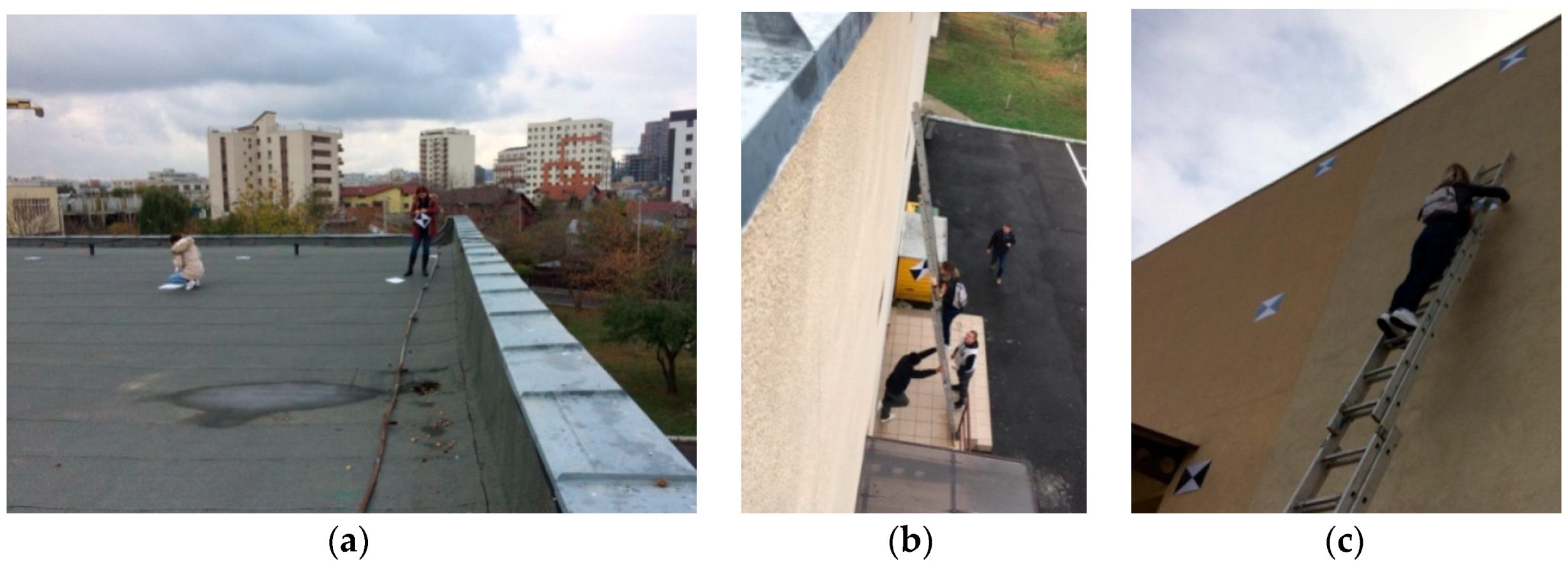
Firstly, 349 uniformly distributed points in the study area were marked: 104 points on the roof (marked with paint, using a plastic pattern), 55 points distributed on 11 rows on the building façade being marked using a construction black marker, 29 points in the green space (reinforced concrete poles to ensure different heights having a metal bold in the superior part), 2 points from the GNSS network (concrete), and 159 points in the parking lot (metallic bolts) (Figure 1).
During the flight, the points marked on the façade and the roof were marked with A3 laminated sheets (Figure 1a–c); after having drawn two black and white triangles, their intersection represented the mathematical point.
The points were situated in the parking lot and the green space, have been marked with plates made by orange plexiglass and two black triangles, 3 mm thickness, 40 cm × 40 cm dimension, with a hole in the center of 5 mm diameter.
A perspective view over the 3D calibration field of digital cameras mounted on UASs, can be seen in Figure 2.
2.3. GNSS Measurements
The solution to design a spatial geodetic network determined by GNSS technology has been chosen, providing a homogeneous and unitary precision of all three components of spatial positioning, currently representing the most efficient approach in the development of geodetic networks in ground measurement works.
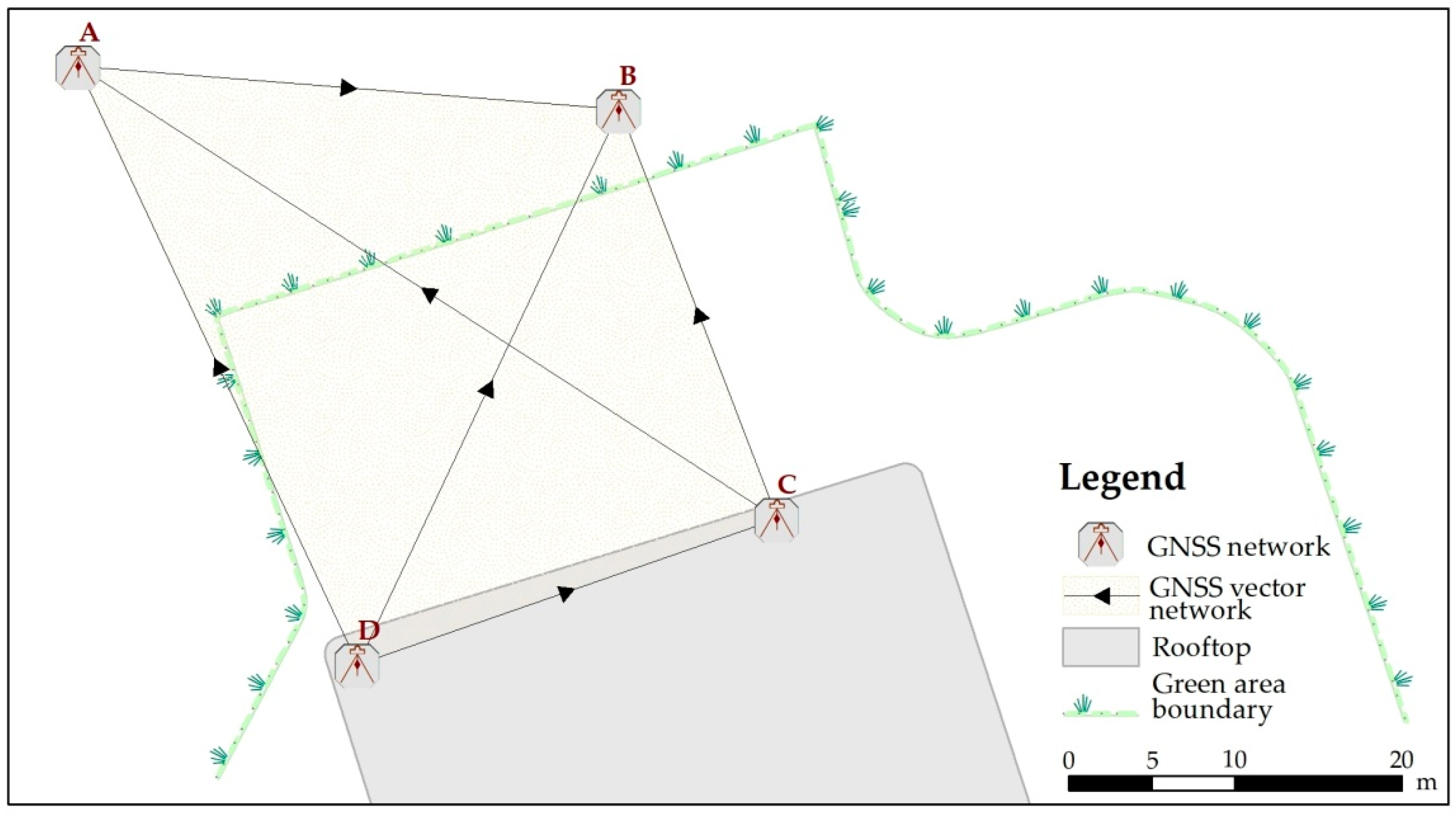
The spatial geodetic network was designed with 4 points (A, B, C, D), two of which (A, B) were grounded in the green area behind the Faculty of Hydrotechnical Engineering, Geodesy, and Environmental Engineering; the other two (C, D) were located on the rooftop, in the northern part of the building at a height difference of about 9 m (Figure 3). In the foregoing research, a local reference and coordinate system was adopted.
The framework of GNSS measurements, is represented by the World Geodetic System (WGS84). The WGS84 is an Earth-centered, Earth-fixed terrestrial reference system and geodetic datum, having three spatial rectangular axes defined in relation with a rotation ellipsoid determined exclusively using data, techniques and satellite technologies.
The GNSS measurements effectuated in the spatial geodetic network were made by static relative positioning method. Three GNSS South S82-V receivers with double frequency GPS + GLONASS + GALILEO + COMPASS + SBAS have been used, having an horizontal precision of positioning of 3 mm ± 0.3 ppm and a vertical precision of 4 mm ± 0.5 ppm, in static mode.
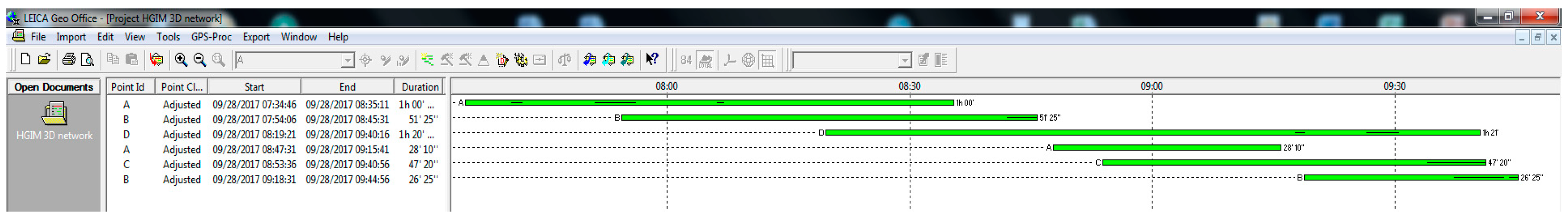
The duration of an observation session is determined by the length of the polygon sides, the number of visible satellites, the geometry of their space position (as assessed by PDOP—Position Dilution of Precision) and the accuracy requirements imposed when determining the network points. Due to distances of less than 50 m between the network points, the duration of a work session was at least 20 min, ranging from 26 min to 1 h and 50 min, i.e., the time period required to resolve ambiguities from phase measurements. After data collection, the receivers were switched off and a part of them were moved as in the measurements scheme on the following bases (A–B–D, A–D–C, D–C–B). The measurements continued afterward (Figure 4).
The measured GNSS bases, fell within the range PDOP 2.2 ÷ 4.2 (<5), HDOP 1.1 ÷ 1.7 (<2) and VDOP 1.8 ÷ 3.9 (<4), which proves a good configuration of satellite geometry with effect on positioning accuracy of GNSS network points.
2.4. Processing the GNSS Measurements
Observations from all sessions were completed in one day (28 September 2017); this is why the precise ephemeris downloaded from the IGS web site were used for processing.
Four stations with unknown coordinates resulted from the network pre-analysis, (12 components of the three-dimensional rectangular coordinates), 9 GNSS bases (27 relative spatial coordinates), and 27 – 12 = 15 network degrees of freedom.
In the case of static measurements, there are several GNSS loops interconnected. For each formed polygon, the algebraic sum of the GNSS base relative coordinates components (ΔX, ΔY, ΔZ) should be zero. A large non-closure in one of the polygons indicates that there is an error of one or more GNSS bases measured in that polygon. In the non-closure analysis report of polygons formed within the GNSS network (Table 1), it can be seen that they are less than 7 mm in planimetric position, and 3 cm in vertical position, with total relative errors in the range 30 ÷ 292 ppm.
The GNSS network adjustment was performed in the WGS84 three-dimensional coordinate system, under the condition of a free geodetic network, in which no element is considered to be fixed, so, a network in which only the measurements to determine the network geometry is established. The adjustment results are shown in Appendix A.
For the current project, a heterogeneous “LOCAL HGIM” reference and coordinate system (CRS) was adopted, consisting of:
- CRS 1: planimetric rectangular coordinates (x,y) in double tangent stereographical projection “Local—HGIM” with WGS84 datum,
- CRS 2: ortometric altitude (H) in local vertical datum with the horizontal reference plan which pases through origin, having the altitude equal with the ellipsoidal height (because of small distances).
The “Local-HGIM” stereographical projection parameters are presented in Table 2, and the adjusted coordinates of GNSS network points in the new heterogenious reference and coordinate system named “LOCAL HGIM”, together with accuracy assessment, are presented in Appendix A.
For the geographical coordinate transformation into rectangular coordinates defined in the “LOCAL HGIM” coordinate system, a Matlab script was created.
2.5. Measurement of Ground Control Points (GCPs)
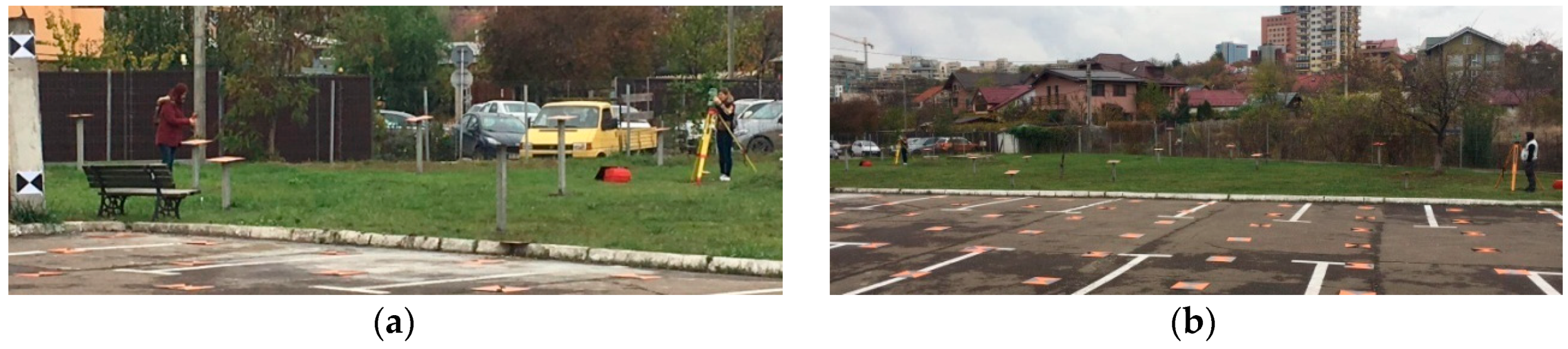
The detail points where determined by topographic measurements using a Leica TCR 405 with an angular precision of 5″ (0.5 mgon) and distance precision of 2 mm + 2 ppm in Fine-Mode (IR). Each GCP have been double measured with a miniprism verticalized with a buble (Figure 5a) from the ends of a GNSS base (A–B for the points situated in the parking lot and the green area (Exhibit 5b) and C–D for the points situated on the roof).
As a preliminary check, the differences were made between the two coordinates strings thus obtained, resulting in a mean absolute value of 9 mm in the horizontal position and 1 mm in the vertical position for the parking and green area points, and 3 mm in the horizontal position and 6 mm in vertical position for the roof points.
For the GCPs coordinate adjustments, the preliminary reduction of slant distances and zenithal angles to the direction between points at ground level was necessary.
At the end of this stage, the initial coordinates of the GCPs were obtained as a simple arithmetic mean between the two above-mentioned determinations, to be included further in the adjustment process, applying the least squares method.
2.6. Geodetic Measurements Processing
The adjustment of the topographic data was made in an application that was specifically developed in the Matlab, having as inputs the GNSS base points coordinates, the initial coordinates of the GCPs, and the topographic elements measured on the ground. To obtain the adjusted spatial coordinates of the GCPs, for each individual point, the adjustment functional model of indirect weight method was applied [25]. The total spatial positioning error for the whole project was less than 5 mm.
2.7. UAS Image Acquisition over the Proposed 3D Calibration Field
For this study, a low-cost UAS “DJI Phantom 3 Standard” was used, with an integrated “GoPro” digital camera (12 Mega pixel) equipped with a 6.31748 mm by 4.73811 mm image sensor. The digital image has a resolution of 4000 × 3000 pixels with a 1.6245 µm pixel size.
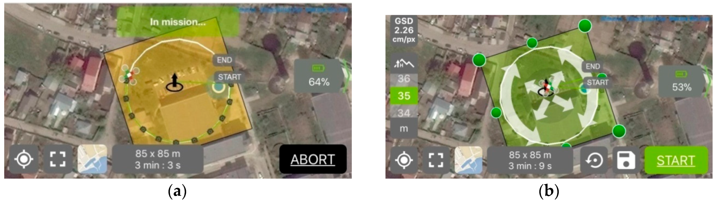
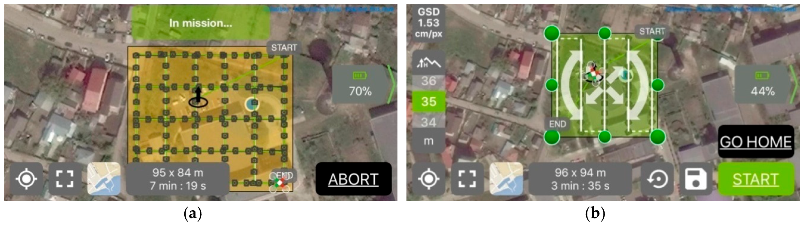
UAS images were taken over the calibration field from 3 different heights: 23 m, 28 m, and 35 m, using the “Pix4D Capture” software for flight planning and control of the UAS system during the flight mission. The “circular” mode for image acquisition was selected for the area of interest (Figure 6a,b).
The image configuration for the camera calibration is close to the one described in [9]. Here, it is mentioned that the test field should be imaged perpendicularly and obliquely, and each image should have a relative rotation of 90° around the optical axis, with eight images being sufficient. As the DJI system has an integrated camera which cannot be separated from the drone itself, taking rotated images in vertical plane around the optical axis is impossible. So, 17 images were taken in an oblique position, the camera being orientated with the optical axis towards the geometric center. Additionally, 4 images in nadiral position were acquired in manual mode with the camera rotated each time at 90° around the optical axis, approximatively above the geometric center, used primarily to determine the principal point coordinates and affinity parameters.
3. Experiments and Results
3.1. UAS Images Processing for Camera Calibration
The camera calibration process was used to obtain intrinsic parameters such as focal distance (f), optical point coordinates (u0,v0), correction of radial distortion (k1, k2, k3), correction of decentering distortion (p1, p2) [1] as well as the extrinsic parameters (rij, X0, Y0, Z0).
The calibration was carried out as part of a bundle block adjustment using the “Pix 4D Mapper” and “3DF Zephyr Pro” software.
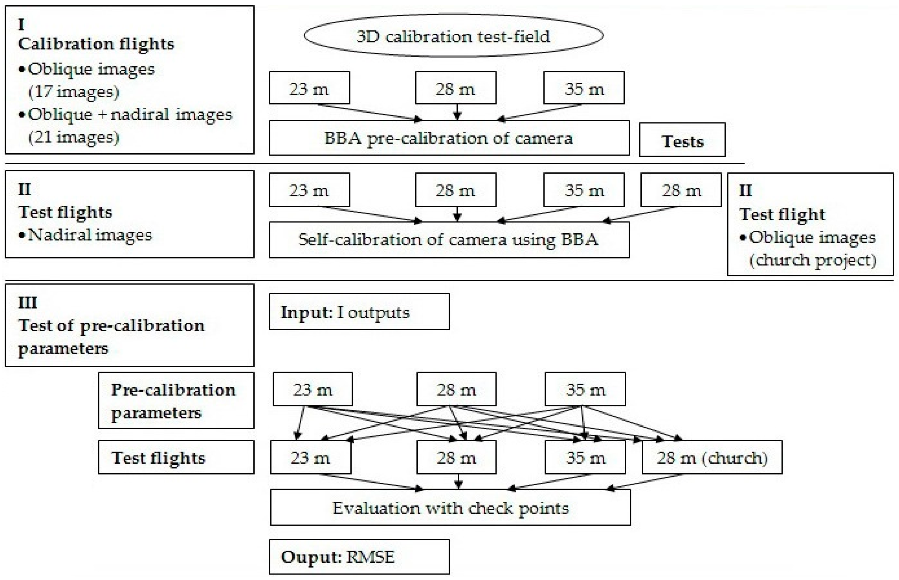
The workflow of this study is presented in Figure 7.
3.1.1. Camera Calibration Using “Pix 4D Mapper” Software
To process the UAS images in “Pix4D Mapper” software, the desired images were imported into a new project, and regarding the “Output/GCP Coordinate System”, the “Arbitrary coordinate system” was selected, the “Image Geolocation” being taken from the EXIF information. With “GCP/MTP Manager”, the file with the control points coordinates was imported, the horizontal accuracy was changed to 0.002, and the vertical accuracy (m) to 0.001, the “Type” of GCP being left as the default, namely “3D GCP”. First, 9 GCP were manually measured on each image using “Basic Editor” for a preliminary image block orientation through BBA.
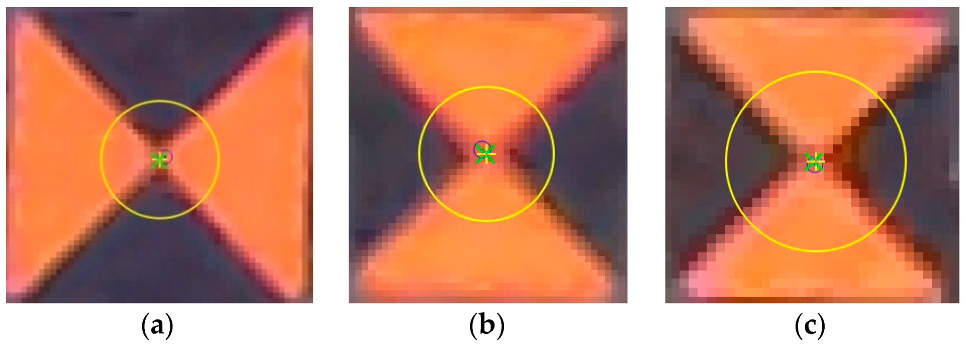
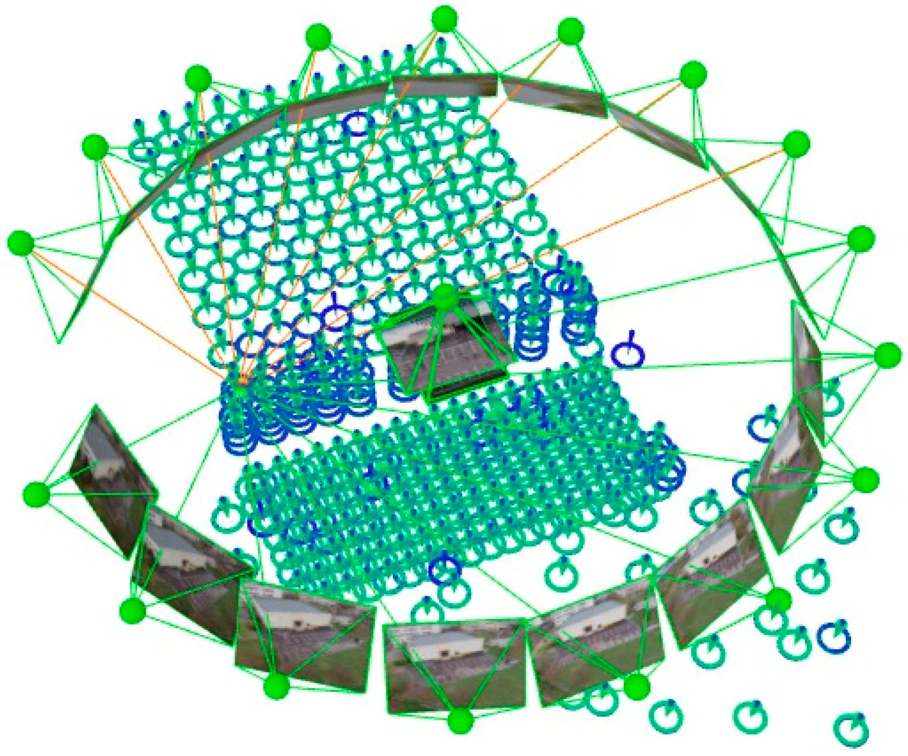
As an advanced processing option, the geometrically verified matching was utilized for the matching strategy, and the “standard” option was selected with all internal and external parameters optimization for the calibration method. After performing the BBA, the images have been oriented and the rest of the 340 GCPs were measured easily on each image as they appeared, the approximate position being indicated by the software after performing a ray intersection (Figure 8). Even so, the GCP marking remains time-consuming for the operator (approximately 8 h).
A final BBA ran and a quality report was created, as well as a graphic representation (Figure 9). The nadiral images haven’t been oriented automatically by the software, so a minimum of 7 GCP was measured on each unoriented image. All GCPs that appear on each nadiral image could be measured after processing again the project.
The principal elements of the quality report for each calibration process for the 3 different heights and the two configurations for image acquisition, 21 images and 17 images respectively, can be found in Table 3.
The values of interior orientation parameters for each case are listed in Table 4, where f is the focal length, u0 and v0 are the coordinates of the principal point, k1, k2 and k3 are the coefficients of the radial distortion, and p1 and p2 are the coefficients of the tangential distortion.
The same measurements for GCPs image coordinates have been used into “3DF Zephyr Pro” software.
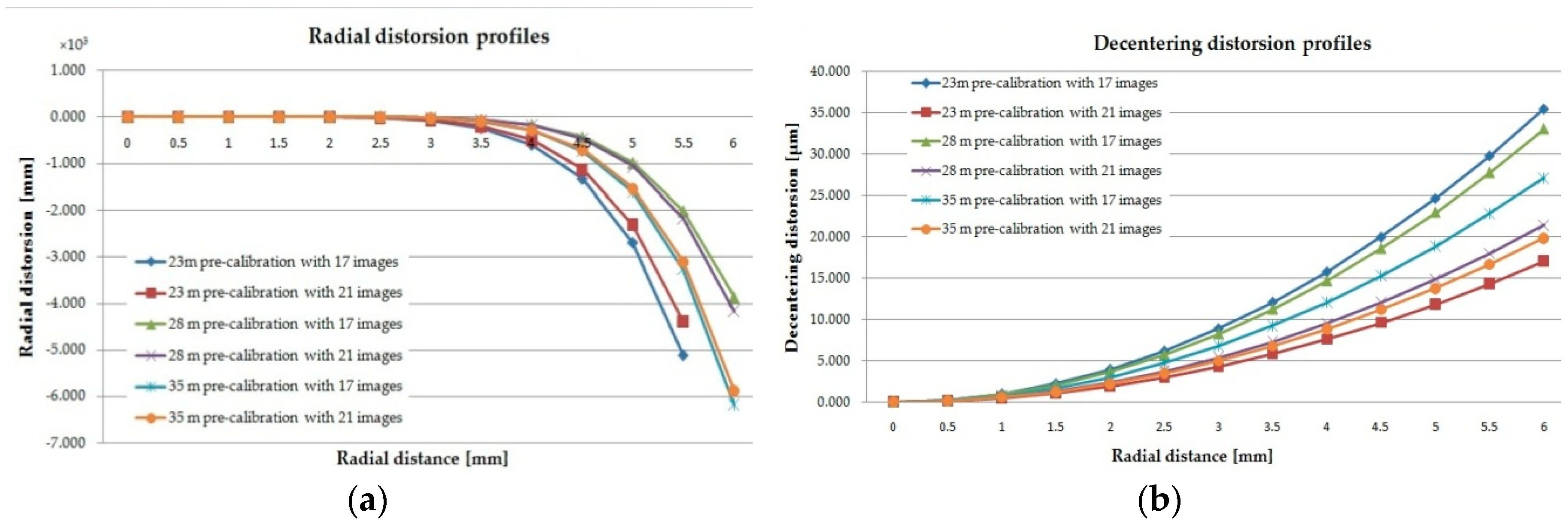
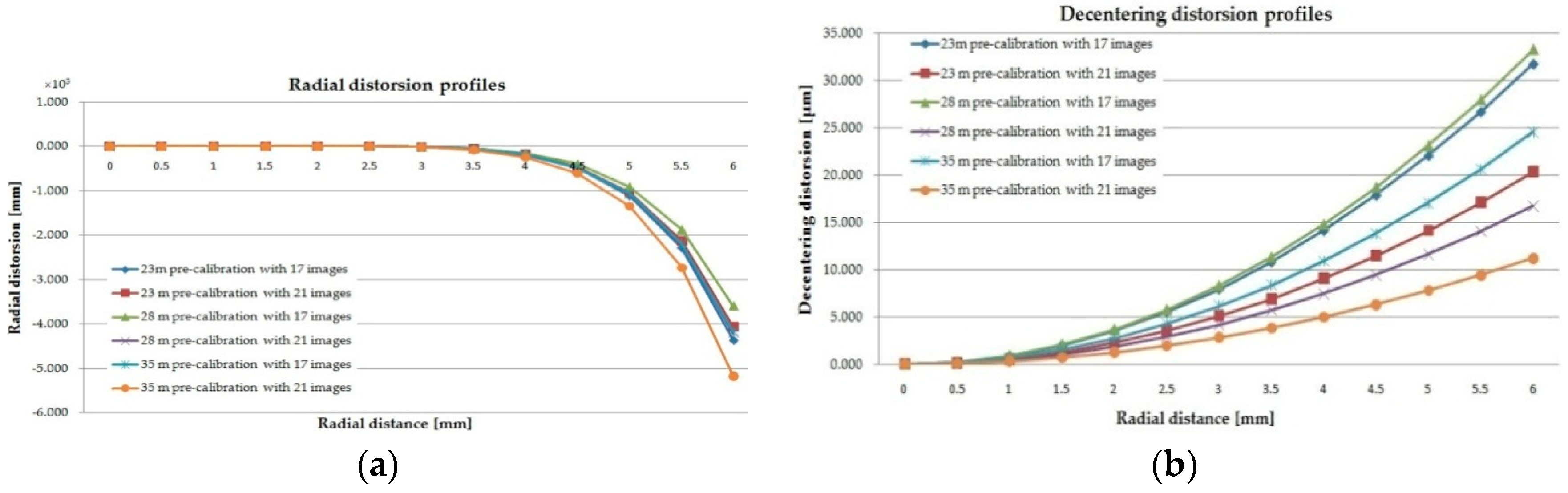
To model the radial distortion Δr, the odd-order polynomial Δr = K1r3 + K2r5 + K3r7 [26,27,28], where r is the radial distance, was used and the radial distortion profiles for all three heights, and for the two image configuration, as shown in Figure 10.
The decentering distortion is due to the lens elements decentering along the optical axis [28], and was graphically represented in an analogous manner to radial distortion, using the function:
3.1.2. Camera Calibration Using “3DF Zephyr Pro” Software
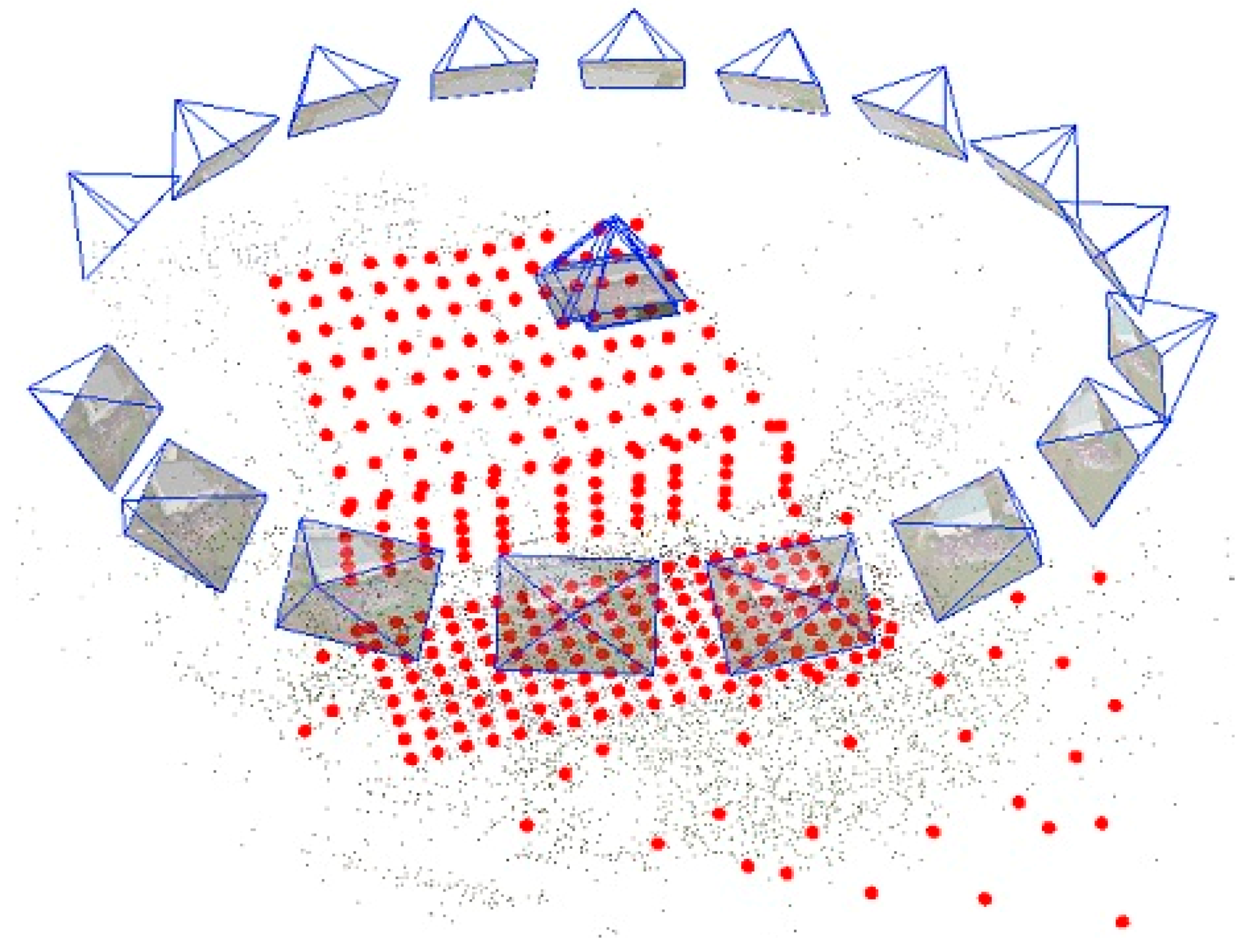
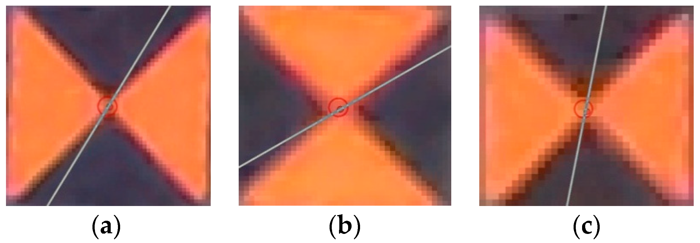
For UAS image processing using the “3DF Zephyr Pro” software, the images were imported into the software and the project was processed without specifying the calibration parameters, so for the interior and exterior orientation parameters for each camera position, an approximation was made based on the EXIF information. After performing SfM process, the image coordinates of each GCP were imported, a preliminary check for each one being made based on the reprojection error to see if all GCPs have been imported correctly. Then, the 3D coordinates have been added. Finally, the “constraint” and “control” boxes have been checked for all 349 GCPs, and a bundle adjustment process was performed adjusting all the interior orientation parameters. After performing BBA, all images have been automatically oriented, and the parameters of interior and exterior orientation have been calculated (Figure 11). If an additional measurement for a GCP is to be made, the correct position on the image is found by a ray intersection (Figure 12).
The principal elements of the quality report for each calibration process done for the 3 different heights in “3DF Zephyr Pro” software and the two configurations for image acquisition, 21 images and 17 images respectively, are listed in Table 5.
The values of interior orientation parameters for each case are listed in Table 6.
The radial and decentering distortion profiles drawn using the coefficients calculated with “3DF Zephyr Pro” software are shown in Figure 13.
3.2. UAS Image Acquisition for Testing the Proposed 3D Calibration Field
In order to test the obtained interior orientation parameters, UAS images were taken with the “DJI Phantom 3 Standard” platform over the calibration field at the same heights as in the camera calibration processes, immediately after the calibration flights. The flight planning was made with “Pix4D Capture” software (Figure 14), choosing the longitudinal and transversal overlap of 80% and 60% respectively, the camera being oriented in nadiral position. For 28 m height, the flight was made in double grid and 122 images were acquired, while for 23 m and 35 m, the flight was made in single grid and 85 and 51 images were acquired respectively.
3.3. UAS Image Processing for Testing the Proposed 3D Calibration Field
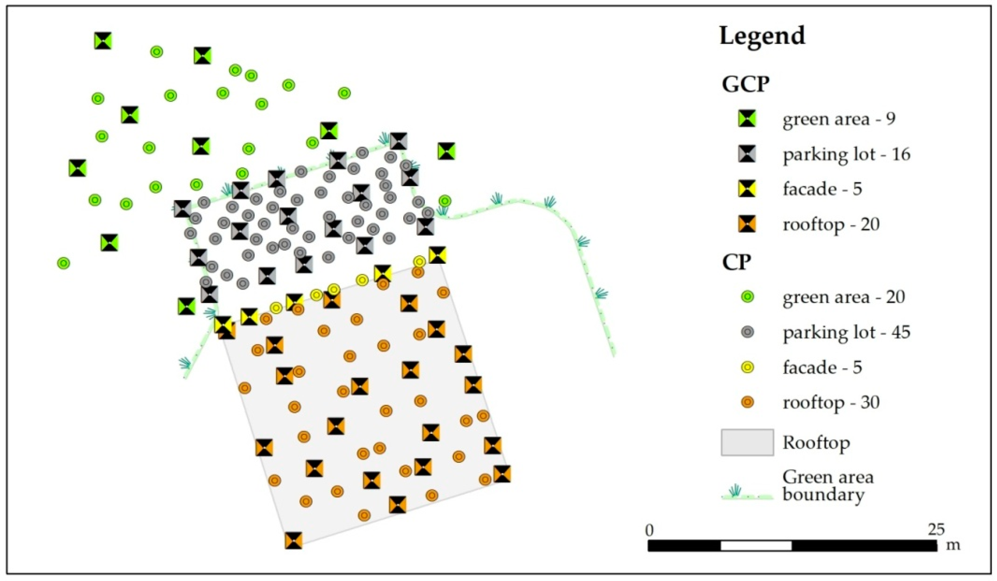
A total of 63 scenarios were tested. The assessed key variables were: (i) the influence of pre- calibration process on the accuracy of BBA in comparison with self-calibration; (ii) the inclusion or exclusion of nadiral images from the image blocks used for the calibration processes; (iii) the influence of height between the calibration process and the UAS reconstruction project; and (iv) the number of GCPs. In order to process the UAS images, the coordinates of 150 points were selected from the total of 349 targets representing the calibration field, 50 of them being considered GCPs and the rest of 100 as Check Points. The distribution of these points can be found in Figure 15.
Before processing UAS images with 3DF Zephyr Pro different scenarios were tested using both “Pix 4D Mapper” and “3DF Zephyr Pro” software. In both cases, a minimum of 3 GCPs were manually measured on each image in which they appeared for a preliminary image block orientation through BBA. Then, the rest of GCPs were measured easily, the approximate position being indicated by the software after performing a ray intersection. We have concluded that even if a point has the “type” changed to “Check Point”, it is included in the BBA. As we wanted to have a set of control points independent of BBA, we tried to make two separate lists of points: one for GCPs, and one for check points (CPs). When using a minimum number of GCPs, the “Pix 4D Mapper” is absolutely wrong when computing the images orientation, so we further replaced the calibration parameters into “3DF Zephyr Pro”.
Quality Assessment
The residuals of the BBA are computed by comparing the CPs coordinates with those determined with high precision followed by the determination of the root mean square error (RMSE). So, the software is using only the points marked as “control” in the BBA process. A different number was used for GCPs: the minimum of 3, the optimum of 14, as found in [29], and a large number of 50.
Although the recovered camera parameters with both software were quite similar, by analyzing the results listed in Table 7, we can see that the errors are smaller in the case of using the calibration parameters calculated with “3DF Zephyr Pro” software. Therefore, we have done further tests using only these parameters.
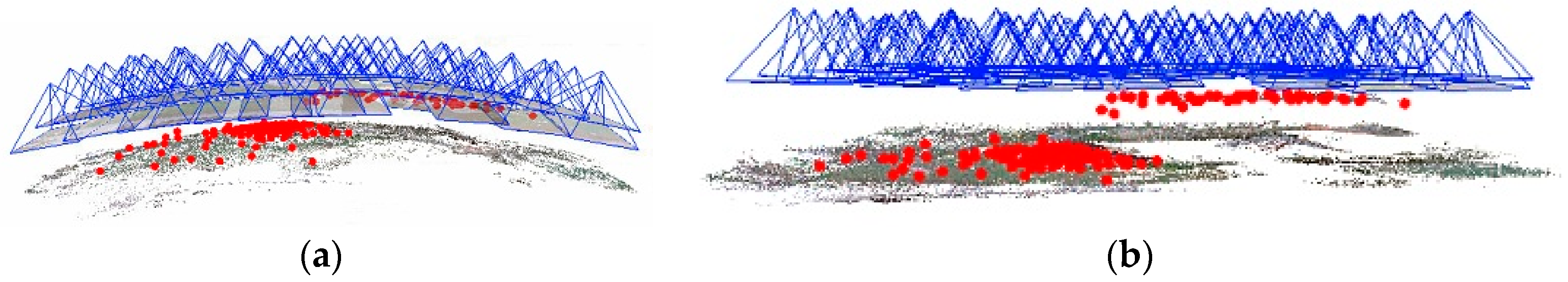
When using self-calibration with the minimum number of GCPs, the errors are very large because the image block is affected by the bowl effects (Figure 16a). By modifying the camera interior orientation parameters before running the SfM, the distortions are corrected (Figure 16b).
In the case of 23 m nadiral block images, not all 100 CPs could be measured on a minimum of 2 images, so only 87 CPs were used to compute the residuals, as shown in Table 8. Also, only 44 GCPs have been used as constraints in the BBA process.
The residuals for the 28 m nadiral flight have been calculated using 100 CPs, and are listed in Table 9. In the case of the 35 m nadiral block images, only 99 CPs were used to compute the residuals, as shown in Table 10.
In Table 8, Table 9 and Table 10, the residuals have also been listed in relation with the value of GSD calculated as a relationship between the flight height and the focal length multiplied by the sensor size. So, for the 23 m height, a value of 0.93 cm was obtained for the GSD; for the 28 m height, a value of 1.1 cm, and for the 35 m, a value of 1.4 cm was obtained.
3.4. Testing the Pre-Calibration Parameters with an Oblique Flight
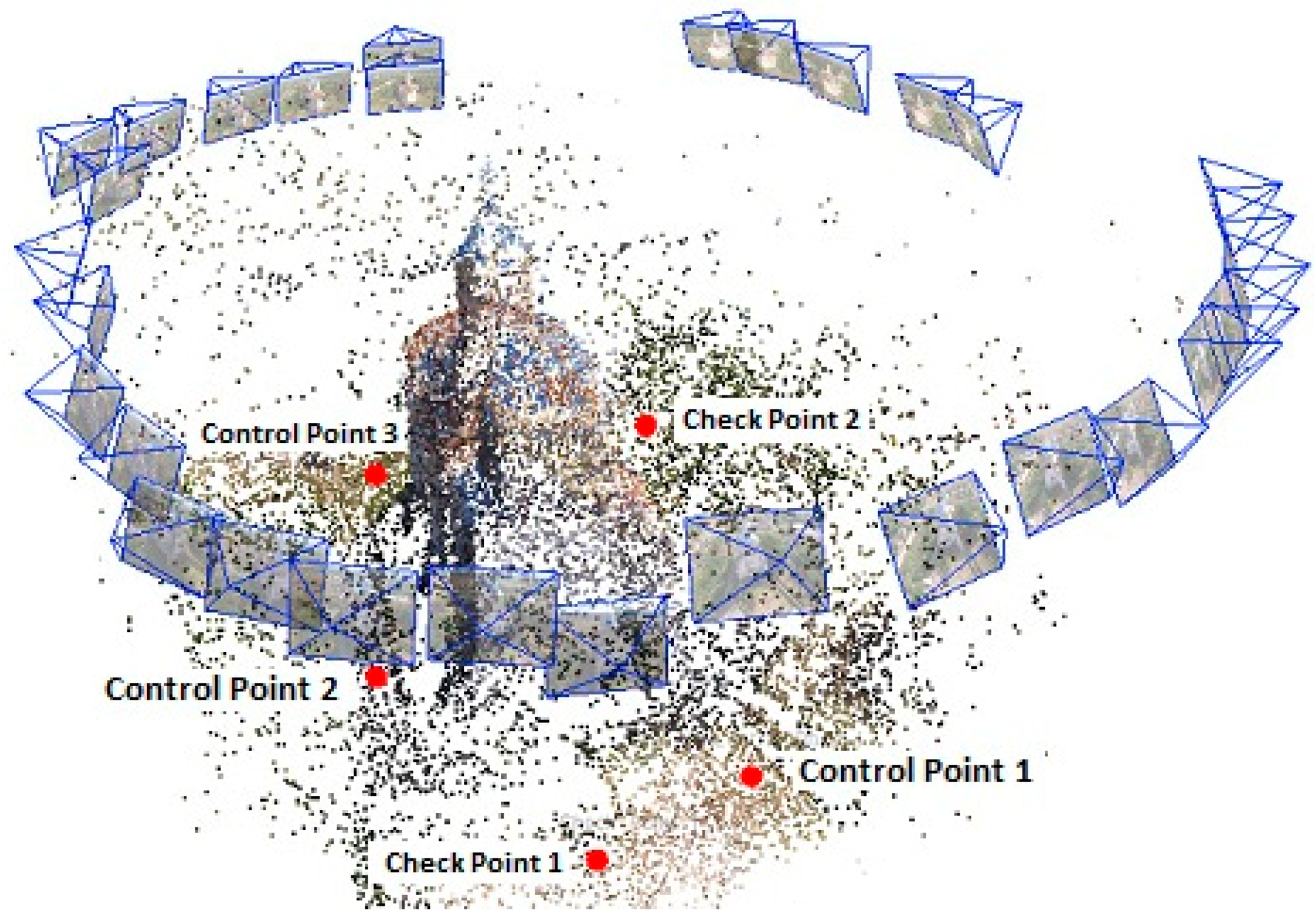
In order to test the pre-calibration parameters on an oblique flight, we chose a UAS reconstruction project done for an old monastery two years before camera calibration. Five reference points were uniformly distributed around the monastery, allowing good visibility without any blockage from vegetation. Three of them have been used as GCPs in order to place the project into a desired coordinate system, i.e., “Stereographical on unique secant plane 1970” and two of them as check points (Figure 17).
The reference points were made by plexiglass, having the center marked by the intersection of two black triangles with 30 cm × 30 cm dimensions. The coordinates were measured with high accuracy using the GNSS technology, the final coordinates resulting as an average of two determinations. For UAS image acquisition, the flight was made in manual mode a total of 30 images from 30 different camera positions being acquired in a circular sequence with the camera axis oriented approximately at 45 degrees to perform oblique acquisition for the facades. Taking into account that the flight was done in manual mode, the altitudes above ground for each camera positions are different, ranging from 25 m to 30 m, with an average of 28 m.
4. Discussion
For this study, a 3D calibration test-field was designed and tested, being the largest reported to date. A number of 349 non-coded targets was measured with millimeter precision in a designed local coordinate system. The camera was calibrated at three different flying heights with two configurations for image acquisition, and the tests were performed on nadiral and oblique flights done at three heights, i.e., 23 m, 28 m, and 35 m, the same as for camera calibration. The pre-calibration parameters were compared with self-calibration parameters, by interchanging the heights after performing a total of 63 scenarios using 3, 14, and 50 GCPs and 100 CPs.
Knowing the camera calibration parameters, after the BBA process, the positions of the measured geometric features are as well adjusted, so the less the RMSE of the CPs object coordinates, the better the distortion parameters were estimated.
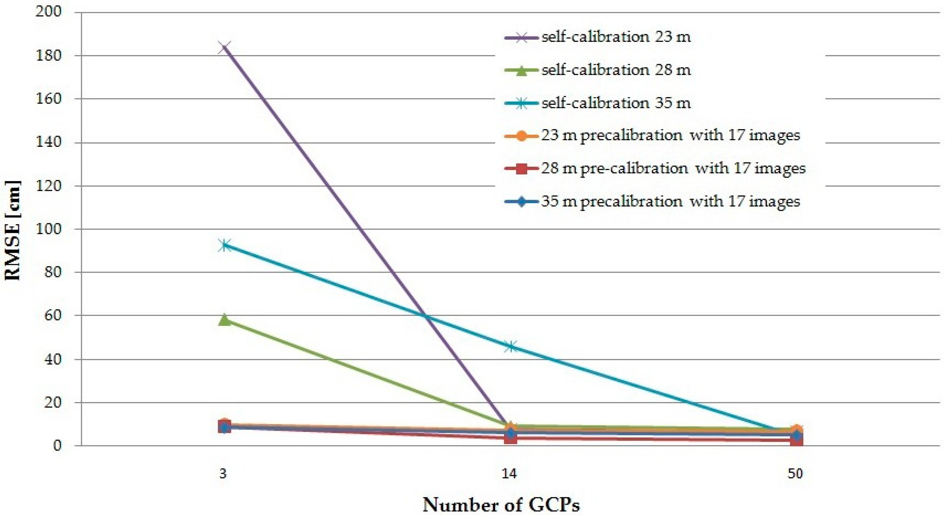
The errors are very large in the case of self-calibration with a minimum number of GCPs. In the case of a double grid nadiral flight, the RMSE is approximately 60 cm, while in the case of a nadiral single grid, the RMSE is 93 cm for the 35 m flight and 1.84 m for 23 m flight. As mentioned in [29,30,31], the errors of a Digital Surface Model (DSM) outside the GCPs area can reach 3 m, so the results support these findings. For all camera blocks, it was found that when the number of control points increases, the accuracy improves, reaching cm- to dm- level positioning accuracy.
The accuracy is improved by 75% when using pre-calibration in the orientation of the double grid nadiral block image with a minimum number of GCPs. When the number of GCPs increase, the accuracy improves by more than 50% (Figure 18).
When using pre-calibration parameters in the orientation of a single grid nadiral block image with a minimum number of GCPs, the accuracy is improved by 95% for the 23 m flight and 90% for the 35 m flight. So, using SfM technique to orient the images and only 3 GCPs in the BBA process, the distortion parameters are poorly-modelled, particularly if the camera network is comprised of traditional nadiral images in strips and blocks [10]. When the optimum and a large number of GCPs are used in the process of BBA of the 23 m flight, the self-calibration led to slightly better results than pre-calibration in the range of 1–5 mm. When the optimum of GCPs is used in the case of 35 m flight, the pre-calibration improved the results by 86%, and the errors have almost the same values when a large number of GCPs i.e., 50, was used. So, using 1 GCP/65 sq. m in the process of BBA, the results of self-calibration and pre-calibration converge.
Even if a large number of GCPs are used for orienting a double grid nadiral flight, pre-calibration improves the results with respect to self-calibration with more than 50% in comparison with single grid, because good coverage of the study area is assured. So, having a pre-calibrated camera along with good image configuration and an optimal number of GCPs, an accuracy of half decimeter can be achieved. The impact of pre-calibration when using a large number of GCPs isn’t so notable in the case of single grid, taking into account the side overlap of 40% and the fact that the roof has a uniform texture and it covers approximately 15% of the study area.
Orthogonal roll angles must be used to image the test-field for calibration purpose in order to break the projective coupling between interior and exterior orientation parameters, but, using a strongly 3D object point array and higher convergence angles for the images, it is possible to decouple the interior and exterior orientation parameters as mentioned in [7].
Analyzing the residuals when using the two image configuration, 17 oblique images and 21 oblique and nadiral rolled images around the optical axis, we can see for the two single grid nadiral flights that they are slightly different, being better overall in the case of 17 oblique images. Looking at the residuals obtained for the double grid nadiral flight with 17 images camera pre-calibration, they are better in percentage by approximately 35% with respect to self-calibration when using only 3 GCP in the BBA process and 3 ÷ 10% when using the optimum and a large number of GCPs. So, the exclusion of nadiral images from the image blocks used for the calibration process is possible, in agreement with the findings of [7].
In the case of the oblique flight done for an old monastery 2 years before calibration, the accuracy when using the pre-calibration parameters is improved by approximately 60%. The time variation of the interior orientation parameters had no impact on the accuracy of the UAS project even after this long period of time. This can be explained, as Cramer et al. [23] found that the DJI Phantom low-cost UAS system is already close to the concept of the metric camera design after performing a short distance test-field calibration in different epochs.
The smallest residuals computed for the 23 m nadiral flight were obtained using the 23 m pre-calibration height, so the same height for pre-calibration as for the UAS reconstruction project. Analyzing the residuals listed in Table 11 for the 28 m nadiral flight, we can see that better results were obtained when using 35 m pre-calibration height. In addition, analyzing the residuals calculated for the 35 m nadiral flight, the smaller values can be found for the 35 m pre-calibration height. We can conclude that the same height for pre-calibration must be used as for the UAS reconstruction project.
5. Conclusions
Our study assessed the accuracy of image block orientation through BBA process with a focus on the influence of pre-calibrated camera. For this purpose, the calibration parameters for the digital camera integrated into the “DJI Phantom 3 Standard” UAS platform calculated using the proposed test-field calibration and the “3DF Zephyr Pro” software for three different heights, namely 23 m, 28 m, and 35 m, and for two image configurations only with oblique images and with a combination of nadiral and oblique images, have been tested.
For all tests done, in the case of the double grid nadiral flight, the parameters calculated with the proposed 3D field improved the results by more than 50% when using the optimum and a large number of GCPs, and by 75% to 95% when using a minimum of 3 GCP in all other analyzed cases.
If the UAS reconstruction project involves an area with a very rugged terrain, placing the GCPs and check points and measuring their position is a very time-consuming step of the survey, and may be impossible. Since UAS are built for this purpose, namely for imaging areas that are not easily accessible, such situations are not uncommon. Using the pre-calibration parameters, a minimum number of 3 GCP can be used for BBA for obtaining a decimeter precision.
The self-calibration can be used when a number of well distributed GCPs is available and the network geometry is favorable, but the advantages of using test-field calibration are that the accuracy is significantly improved and the number of GCPs is considerable reduced.
This research has investigated the relationship between height for calibration process and the UAS reconstruction project.
It has been shown that the interior orientation parameters calculated for a digital camera integrated in an UAS platform using a test-field calibration can be transferred with success to other UAS reconstruction projects. Also, by testing the interior orientation parameters obtained by using a 3D calibration test-field on UAS projects done before camera calibration (monastery) respectively after camera calibration (nadiral flights), we showed that the UAS cameras can be pre- or post- calibrated.
Further research can be done by performing camera calibration using the OrienTal software developed by Department of Geodesy and Geoinformation from TU WIEN and other commercial software such as Agisoft and Australis.
Author Contributions
Experiment conception and design, V.-E.O. and N.P.; Methodology, V.-E.O.; Processing of UAS images, V.-E.O. and A.-M.L.; Validation, V.-E.O., N.P. and A.-M.L.; Formal Analysis, V.-E.O.; Investigation, V.-E.O. and N.P.; Resources, V.-E.O. and A.-M.L.; Writing—Original Draft Preparation, V.-E.O.; Writing—Review & Editing, N.P.; Visualization, A.-M.L.; Supervision, N.P.
Funding
This research received no external funding.
Acknowledgments
This work was supported by a grant of the Romanian Ministry of Research and Innovation, CCCDI-UEFISCDI, project number PN-III-P2-2.1-CI-2017-0623, within PNCDI III. No funds have been received for covering the costs to publish in open access.
Conflicts of Interest
The authors declare no conflict of interest.
Appendix A

Table A1.
The adjusted coordinates of GNSS network points.
| Point | Adjusted WGS84 Cartesian Coordinates | Adjusted WGS84 Geodetic Coordinates | ||||
|---|---|---|---|---|---|---|
| X (m) | Y (m) | Z (m) | B (° ′ ″) | L (° ′ ″) | HE (m) | |
| A | 3,850,635.6259 | 2,012,904.9023 | 4,653,646.0581 | 47 09 22.44280 | 27 35 53.32127 | 72.3272 |
| B | 3,850,622.9236 | 2,012,933.389 | 4,653,644.4446 | 47 09 22.36121 | 27 35 54.79906 | 72.4634 |
| C | 3,850,639.011 | 2,012,952.0451 | 4,653,634.5178 | 47 09 21.59893 | 27 35 55.23012 | 80.7569 |
| D | 3,850,655.4025 | 2,012,933.3896 | 4,653,628.4944 | 47 09 21.32661 | 27 35 54.08480 | 80.3415 |
Table A2.
The adjusted coordinates of GNSS network points in CRS—“LOCAL HGIM”.
| Point | Planimetric Rectangular Coordinates “Local-HGIM”/WGS84 | Ortometric Altitudine | Standard Deviation | |||
|---|---|---|---|---|---|---|
| x (m) | y (m) | H (m) | sx (m) | sy (m) | sH (m) | |
| A | 1014.9097 | 980.6469 | 72.3272 | 0.0011 | 0.0007 | 0.0077 |
| B | 1012.3900 | 1011.7766 | 72.4634 | 0.0013 | 0.0009 | 0.0123 |
| C | 988.8496 | 1020.8570 | 80.7569 | 0.0012 | 0.0007 | 0.0072 |
| D | 980.4399 | 996.7307 | 80.3415 | 0.0008 | 0.0005 | 0.0060 |
References
- Zhang, Z. A flexible new technique for camera calibration. IEEE Trans. Pattern Anal. Mach. Intell. 2000, 22, 1330–1334. [Google Scholar] [CrossRef] [Green Version]
- Samper, D.; Santolaria, J.; Brosed, F.J.; Majaren, A.C.; Aguilar, J.J. Analysis of Tsai calibration method using two and three-dimensional calibration objects. Mach. Vis. Appl. 2013, 24, 117–131. [Google Scholar] [CrossRef]
- Oniga, V.E.; Oniga, M.B. Testing the accuracy of different calibration methods. J. Geod. Cartogr. Cadastre 2015, 2, 8–17. [Google Scholar]
- Loghin, A.M.; Oniga, V.E. The influence of camera calibration parameters on 3D buildings models creation. J. Geod. Cadastre Rev. CAD 2014, 17, 178–185. [Google Scholar]
- Oniga, V.E.; Chirila, C. Object based digital non-metric images accuracy. In Proceedings of the 13th International Multidisciplinary Scientific Geo Conference, Albena, Bulgaria, 16–22 June 2013; Volume II, pp. 655–662. [Google Scholar]
- Förstner, W.; Wrobel, B.; Paderes, F.; Craig, R.; Fraser, C.; Dolloff, J. Analytical Photogrammetric Operations, ASPRS Manual of Photogrammetry, 5th ed.; McGlone, J.C., Mikhail, E., Bethel, J., Eds.; American Society for Photogrammetry and Remote Sensing: Bethesda, MD, USA, 2004; pp. 763–936. ISBN 978-1570830716. [Google Scholar]
- Remondino, F.; Fraser, C. Digital Camera Calibration Methods: Considerations and Comparisons. In Proceedings of the ISPRS Commission V Symposium ‘Image Engineering and Vision Metrology’, Dresden, Germany, 25–27 September 2006; Volume 36, pp. 266–272. [Google Scholar]
- Zhang, Z. Camera Calibration. In Emerging Topics in Computer Vision; Medioni, G., Kang, S.B., Eds.; Prentice Hall Professional Technical Reference: Upper Saddle River, NJ, USA, 2004; pp. 4–43. [Google Scholar]
- Luhmann, T.; Robson, S.; Kyle, S.; Harley, I. Measurement concepts and solutions in practice. In Close-Range Photogrammetry. Principle, Methods and Applications; Whittles: Scotland, UK, 2006; pp. 448–458. ISBN 1–870325-50–8. [Google Scholar]
- Harwin, S.; Lucieer, A.; Osborn, J. The impact of the calibration method on the accuracy of point clouds derived using unmanned aerial vehicle multi-view stereopsis. Remote Sens. 2015, 7, 11933–11953. [Google Scholar] [CrossRef]
- Honkavaara, E.; Ahokas, E.; Hyyppä, J.; Jaakkola, J.; Kaartinen, H.; Kuittinen, R.; Markelin, L.; Nurminen, K. Geometric test field calibration of digital photogrammetric sensors. ISPRS J. Photogramm. Remote Sens. 2006, 60, 387–399. [Google Scholar] [CrossRef]
- Fryer, J.G. Camera calibration in non-topographic photogrammetry. In Non-Topographic Photogrammetry, 2nd ed.; American Society for Photogrammetry and Remote Sensing: Falls Church, VA, USA, 1989; p. 64. [Google Scholar]
- Hieronymus, J. Comparison of methods for geometric camera calibration. In Proceedings of the XXII ISPRS Congress International Archives of the Photogrammetry, Remote Sensing and Spatial Information Sciences, Melbourne, Australia, 25 August–1 September 2012; pp. 595–599. [Google Scholar]
- Balletti, C.; Guerra, F.; Tsioukas, V.; Vernier, P. Calibration of Action Cameras for Photogrammetric Purposes. Sensors 2014, 14, 17471–17490. [Google Scholar] [CrossRef] [PubMed] [Green Version]
- Pérez, M.; Agüera, F.; Carvajal, F. Digital Camera Calibration Using Images Taken From an Unmanned Aerial Vehicle. In Proceedings of the Unmanned Aerial Vehicle in Geomatics, Zurich, Switzerland, 14–16 September 2011; Volume XXXVIII-1/C22, pp. 1–5. [Google Scholar]
- Chiang, K.W.; Tsai, M.L.; Naser, E.S.; Habib, A.; Chu, C.H. New calibration method using low cost MEMS IMUs to verify the performance of UAV-borne MMS payloads. Sensors 2015, 15, 6560–6585. [Google Scholar] [CrossRef] [PubMed]
- Toschi, I.; Rivola, R.; Bertacchini, E.; Castagnetti, C.; Dubbini, M.; Capra, A. Validation test of open source procedures for digital camera calibration and 3D image based modeling. ISPRS Int. Arch. Photogramm. Remote Sens. Spatial Inf. Sci. 2013, 1, 647–652. [Google Scholar] [CrossRef]
- Murtiyoso, A.; Grussenmeyer, P.; Freville, T. Close Range UAV Accurate Recording and Modeling of St-Pierre-le-Jeune Neo-Romanesque Church in Strasbourg (France). ISPRS Int. Arch. Photogramm. Remote Sens. Spat. Inf. Sci. 2017, XLII-2/W3, 519–526. [Google Scholar] [CrossRef]
- Yanagi, H.; Chikatsu, H. Camera calibration in 3D modelling for UAV application. Int. Arch. Photogramm. Remote Sens. Spat. Inf. Sci. 2015, XL-4(W5), 223–226. [Google Scholar] [CrossRef]
- Yusoff, A.R.; Ariff, M.F.; Idris, K.M.; Majid, Z.; Chong, A.K. Camera calibration accuracy at different UAV flying heights. Int. Arch. Photogramm. Remote Sens. Spat. Inf. Sci. 2017, 42, 595. [Google Scholar] [CrossRef]
- Honkavaara, E.; Markelin, L.; Ilves, R.; Savolainen, P.; Vilhomaa, J.; Ahokas, E.; Jaakkola, J.; Kaartinen, H. In-flight performance evaluation of digital photogrammetric sensors. In Proceedings of the ISPRS Hannover Workshop, Hannover, Germany, 17–20 May 2005. [Google Scholar]
- Kraft, T.; Geßner, M.; Meißner, H.; Przybilla, H.J.; Gerke, M. Introduction of a photogrammetric camera system for RPAS with highly accurae GNSS/IMU information for standardized workflows. In Proceedings of the EuroCOW 2016, the European Calibration and Orientation Workshop, Lausanne, Switzerland, 10–12 February 2016. [Google Scholar]
- Cramer, M.; Przybilla, H.-J.; Zurhorst, A. UAV cameras: Overview and geometric calibration benchmark. Int. Arch. Photogramm. Remote Sens. Spatial Inf. Sci. 2017, XLII-2/W6, 85–92. [Google Scholar] [CrossRef]
- Shortis, M.R.; Clarke, T.A.; Short, T. A Comparison of Some Techniques for The Subpixel Location of Discrete Target Images. SPIE Proc. 1994, 2350, 239–250. [Google Scholar]
- Ahn, S.J.; Warnecke, H.J.; Kotowskis, R. Systematic Geometric image Measurement Errors of Circular Object Targets: Mathematical Formulation and Correction. Photogramm. Rec. 1999, 16, 485–502. [Google Scholar] [CrossRef]
- Ghilani, C.D.; Wolf, P.R. Adjustment computations. In Spatial Data Analysis, 4th ed.; John Wiley&Sons Inc.: Hoboken, NJ, USA, 2006. [Google Scholar]
- Brown, D.C. Close-range camera calibration. Photogramm. Eng. 1996, 37, 855–866. [Google Scholar]
- Light, D.L. The new camera calibration system at the U.S. Geological Survey. Photogramm. Eng. Remote Sens. 1992, 58, 185–188. [Google Scholar]
- Mugnier, C.J.; Forstner, W.; Wrober, B.; Padres, F.; Munjy, R. The mathematics of photogrammetry. In Manual of Photogrammetry, 5th ed.; McGlone, J.C., Mikhail, E., Bethel, J., Eds.; American Society of Photogrammetry and Remote Sensing: Bethesda, MD, USA, 2004; pp. 181–316. [Google Scholar]
- Oniga, V.E.; Breaban, A.I.; Statescu, F. Determining the Optimum Number of Ground Control Points for Obtaining High Precision Results Based on UAS Images. Proceedings 2018, 2, 352. [Google Scholar] [CrossRef]
- Jaud, M.; Passot, S.; Le Bivic, R.; Delacourt, C.; Grandjean, P.; Le Dantec, N. Assessing the Accuracy of High Resolution Digital Surface Models Computed by PhotoScanR and MicMacR in Sub-Optimal Survey Conditions. Remote Sens. 2016, 8, 465. [Google Scholar] [CrossRef]
Figure 1.
Marking the ground control points (a) on the building roof, (b) and (c) on the facade.

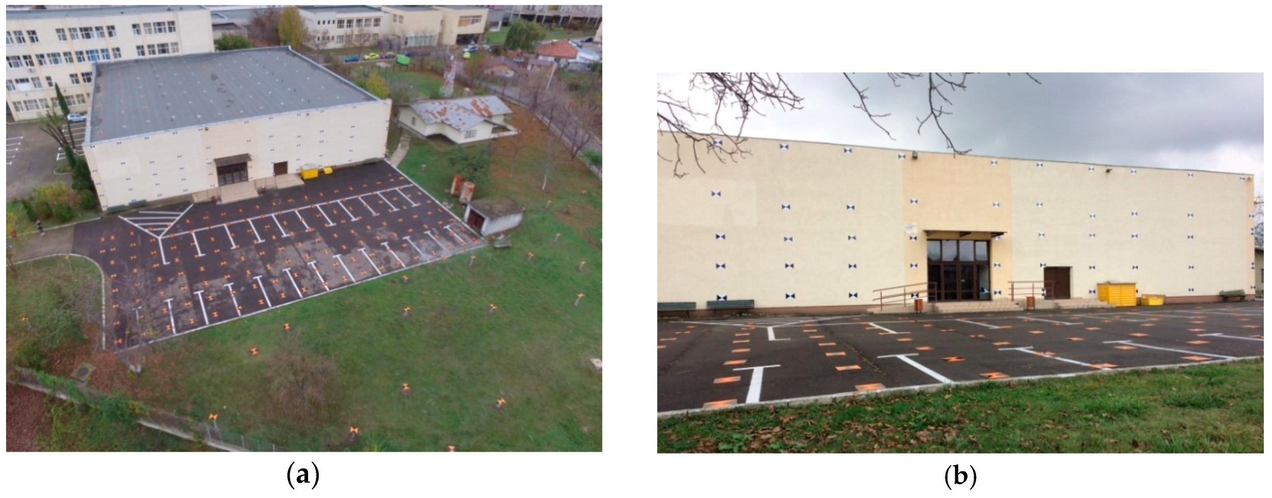
Figure 2.
(a) UAS image over the 3D calibration field of digital non-metric cameras mounted on Unmanned Aerial Systems, (b) ground image.
Figure 2.
(a) UAS image over the 3D calibration field of digital non-metric cameras mounted on Unmanned Aerial Systems, (b) ground image.

Figure 3.
GNSS network.

Figure 4.
GNSS observations sessions.

Figure 5.
(a) Taking the measurements using a miniprism and (b) two Leica TCR 405 total stations, centered on A and B GNSS points.
Figure 5.
(a) Taking the measurements using a miniprism and (b) two Leica TCR 405 total stations, centered on A and B GNSS points.

Figure 6.
Screen shots during the UAS image acquisition over the 3D calibration field for digital cameras mounted on UAS platforms at (a) 28 m height and (b) 35 m height.
Figure 6.
Screen shots during the UAS image acquisition over the 3D calibration field for digital cameras mounted on UAS platforms at (a) 28 m height and (b) 35 m height.

Figure 7.
Experiments workflow.

Figure 8.
Screen shots with a control point image in Pix 4D Mapper (No. 229) positioned approximatively in the calibration field center (a) 23 m height, (b) 28 m and (c) 35 m height.
Figure 8.
Screen shots with a control point image in Pix 4D Mapper (No. 229) positioned approximatively in the calibration field center (a) 23 m height, (b) 28 m and (c) 35 m height.

Figure 9.
The elements resulted after the bundle adjustment process: cameras positions and orientations, GCPs positions and errors marked with green arrow.
Figure 9.
The elements resulted after the bundle adjustment process: cameras positions and orientations, GCPs positions and errors marked with green arrow.

Figure 10.
(a) Radial and (b) decentering distortion profiles for the digital camera mounted on “DJI Phantom 3 standard” UAS at 23, 28, and 35 m height for 17 oblique images and 21 oblique and nadiral images.
Figure 10.
(a) Radial and (b) decentering distortion profiles for the digital camera mounted on “DJI Phantom 3 standard” UAS at 23, 28, and 35 m height for 17 oblique images and 21 oblique and nadiral images.

Figure 11.
The elements resulted after the bundle adjustment process: cameras positions and orientations, GCPs positions and sparse point cloud.
Figure 11.
The elements resulted after the bundle adjustment process: cameras positions and orientations, GCPs positions and sparse point cloud.

Figure 12.
Screen shots with a GCP image in “3DF Zephyr Pro” software (No. 229) positioned approximatively in the calibration field center (a) 23 m height, (b) 28 m and (c) 35 m height.
Figure 12.
Screen shots with a GCP image in “3DF Zephyr Pro” software (No. 229) positioned approximatively in the calibration field center (a) 23 m height, (b) 28 m and (c) 35 m height.

Figure 13.
(a) Radial and (b) decentering distortion profiles for the digital camera mounted on “DJI Phantom 3 Standard” UAS at 23, 28 and 35 m height for 17 oblique images and 21 oblique and nadiral images.
Figure 13.
(a) Radial and (b) decentering distortion profiles for the digital camera mounted on “DJI Phantom 3 Standard” UAS at 23, 28 and 35 m height for 17 oblique images and 21 oblique and nadiral images.

Figure 14.
Taking the UAS images over the calibration field at (a) 28 m and (b) 35 m.

Figure 15.
The 50 GCPs and 100 CPs distribution.

Figure 16.
Images and tie points positions for the 23 m nadiral flight after the orientation process using (a) SfM method and (b) pre-calibration parameters.
Figure 16.
Images and tie points positions for the 23 m nadiral flight after the orientation process using (a) SfM method and (b) pre-calibration parameters.

Figure 17.
The elements resulted after the bundle adjustment process: cameras positions and orientations and GCPs and CPs positions.
Figure 17.
The elements resulted after the bundle adjustment process: cameras positions and orientations and GCPs and CPs positions.

Figure 18.
The RMSE resulted for the 23 m, 28 m, and 35 m flights when using self-calibration and pre-calibration with oblique images.
Figure 18.
The RMSE resulted for the 23 m, 28 m, and 35 m flights when using self-calibration and pre-calibration with oblique images.

Table 1.
The non-closures calculation of GNSS network polygons.
| No. | Polygons | Errors of Closers in Polygons (m) | Length of Polygon | |||
|---|---|---|---|---|---|---|
| e_EST | e_NORTH | e_H | et | Lt (m) | ||
| 1 | D–B–C | 0.0048 | 0.0023 | −0.0163 | 0.0172 | 88.2947 |
| 2 | C–B–A | −0.0060 | 0.0024 | 0.0304 | 0.0310 | 106.4422 |
| 3 | D–C–A | −0.0002 | 0.0010 | −0.0033 | 0.0034 | 113.0794 |
Table 2.
“Local-HGIM” stereographical projection parameters.
| Parameter | Value |
|---|---|
| Latitudine of natural origin (real) | φo = 47°09′21.96″ (north latitudine) |
| Longitudine of natural origin (real) | λo = 27°35′54.24″ (east longitudine) |
| Scale factor | Ko = 1 (tangential projection) |
| False north (translated coordinates of natural origin) | No = Xo = 1000.000 m |
| False east (translated coordinates of natural origin) | Eo = Yo = 1000.000 m |
Table 3.
Summary of full bundle adjustment (BBA) quality report.
| Height (m) | 23 | 28 | 35 | |||
|---|---|---|---|---|---|---|
| No. images | 21 | 17 | 21 | 17 | 21 | 17 |
| Mean GSD (cm) | 3.9 | 3.6 | 2.6 | 2.7 | 2.1 | 2.3 |
| Mean RMSE (mm) | 9 | 8 | 6 | 6 | 6 | 6 |
| Mean reprojection error (pixels) | 0.215 | 0.239 | 0.182 | 0.231 | 0.205 | 0.243 |
| Number of 2D keypoint observations for BBA | 42,078 | 77,507 | 47,166 | 81,841 | 88,266 | 110,229 |
| Mean number of matched 2D keypoint per image | 2004 | 4559 | 2246 | 4814 | 4203 | 6484 |
| Number of 3D points for BBA | 19,216 | 34,893 | 22,343 | 34,455 | 37,202 | 41,473 |
Table 4.
Interior orientation parameters calculated for the “GoPro” digital camera at 3 different heights: 23 m, 28 m and 35 m using “Pix 4D Mapper”software.
Table 4.
Interior orientation parameters calculated for the “GoPro” digital camera at 3 different heights: 23 m, 28 m and 35 m using “Pix 4D Mapper”software.
| Height (m) | No. of Images | f (mm)/pixels | u0 (mm)/(pixels) | v0 (mm)/(pixels) | k1 | k2 | k3 | p1 × 10−4 | p2 × 10−4 |
|---|---|---|---|---|---|---|---|---|---|
| 23 | 21 | 4.27808 | 3.11761 | 2.32975 | −0.129361 | 0.110143 | −0.018652 | −2.3613 | 4.11071 |
| 2708.73 | 1973.96 | 1475.11 | |||||||
| 17 | 4.27885 | 3.12531 | 2.32776 | −0.130439 | 0.113851 | −0.021348 | −2.01641 | 9.64783 | |
| 2709.21 | 1978.83 | 1473.85 | |||||||
| 28 | 21 | 4.27674 | 1974.82 | 1476.65 | −0.129152 | 0.108773 | −0.017812 | −1.91946 | 5.62797 |
| 2707.87 | |||||||||
| 17 | 4.27991 | 3.12421 | 2.32587 | −0.128664 | 0.108156 | −0.016712 | −1.9623 | 8.96893 | |
| 2709.89 | 1978.14 | 1472.65 | |||||||
| 35 | 21 | 4.27975 | 3.11853 | 2.33246 | −0.131715 | 0.116669 | −0.024146 | −2.19276 | 5.06711 |
| 2709.78 | 1974.54 | 1476.83 | |||||||
| 17 | 4.28529 | 3.1219 | 2.32524 | −0.131707 | 0.117748 | −0.025275 | −1.31255 | 7.42829 | |
| 2713.29 | 1976.67 | 1472.26 |
Table 5.
Summary of full bundle block adjustment (BBA) quality report.
| Height (m) | 23 | 28 | 35 | |||
|---|---|---|---|---|---|---|
| No. of images | 21 | 17 | 21 | 17 | 21 | 17 |
| Mean GSD (cm) | 1.6 | 1.8 | 1.9 | 2.0 | 1.7 | 1.9 |
| Mean RMSE (mm) | 11 | 11 | 9 | 9 | 10 | 10 |
| Mean reprojection error (pixels) | 0.572 | 0.542 | 0.501 | 0.276 | 0.604 | 0.290 |
| 3D points per image | 596 | 582 | 1537 | 632 | 1510 | 1017 |
| Number of 3D points for BBA | 5265 | 4330 | 11,877 | 10,758 | 11,659 | 7330 |
Table 6.
Interior orientation parameters calculated for the “GoPro” digital camera at 3 different heights: 23 m, 28 m, and 35 m using “3DF Zephyr Pro” software.
Table 6.
Interior orientation parameters calculated for the “GoPro” digital camera at 3 different heights: 23 m, 28 m, and 35 m using “3DF Zephyr Pro” software.
| Height (m) | No. of Images | f (mm)/pixels | u0 (mm)/(pixeli) | v0 (mm)/(pixeli) | k1 | k2 | k3 | p1 × 10−4 | p2 × 10−4 |
|---|---|---|---|---|---|---|---|---|---|
| 23 | 21 | 2707.326 | 1974.823 | 1477.729 | −0.12940 | 0.109243 | −0.017431 | −2.1990 | 5.2146 |
| 17 | 2710.399 | 1978.085 | 1472.805 | −0.13008 | 0.118661 | −0.018778 | −1.1667 | 8.7533 | |
| 28 | 21 | 2707.599 | 1973.953 | 1477.729 | −0.12983 | 0.109752 | −0.017975 | −1.5643 | 4.3785 |
| 17 | 2709.921 | 1978.267 | 1472.582 | −0.12837 | 0.107149 | −0.015723 | −1.8728 | 9.0569 | |
| 35 | 21 | 2709.367 | 1972.562 | 1476.918 | −0.13098 | 0.113706 | −0.021533 | −1.9484 | 2.4395 |
| 17 | 2710.847 | 1975.954 | 1474.430 | −0.12919 | 0.109489 | −0.017830 | −1.7114 | 6.6117 |
Table 7.
The residuals of 100 CPs for a 28 m nadiral flight when using self-calibration and pre-calibration at 28 m height done with “Pix 4D Mapper” respectively “3DF Zephyr”.
Table 7.
The residuals of 100 CPs for a 28 m nadiral flight when using self-calibration and pre-calibration at 28 m height done with “Pix 4D Mapper” respectively “3DF Zephyr”.
| Height for Pre-Calibration (m) | No. of GCPs | Self-Calibration 28 m Height RMSE (cm) | Pre-Calibration with 17 Images RMSE (cm) | |
|---|---|---|---|---|
| Pix4D Mapper | 3DF Zephyr Pro | |||
| 28 | 3 | 58.4 | 13.7 | 9.0 |
| 14 | 9.1 | 4.31 | 4.11 | |
| 50 | 7.6 | 3.29 | 2.95 | |
Table 8.
The residuals of 87 CPs for a 23 m nadiral flight when using self-calibration and pre-calibration at 3 different heights: 23 m, 28 m and 35 m with two image configuration in the case of a different number of GCPs.
Table 8.
The residuals of 87 CPs for a 23 m nadiral flight when using self-calibration and pre-calibration at 3 different heights: 23 m, 28 m and 35 m with two image configuration in the case of a different number of GCPs.
| Height for Pre-Calibration (m) | No. of GCPs | Self-Calibration 23 m Height RMSE (cm) and RMSE/GSD | Pre-Calibration RMSE (cm) and RMSE/GSD | |
|---|---|---|---|---|
| 21 Images | 17 Images | |||
| 23 | 3 | 184/197.8 | 10.1/10.9 | 10/10.8 |
| 14 | 7.8/8.4 | 7.7/8.3 | 7.7/8.3 | |
| 50 | 6.5/7.0 | 7.0/7.5 | 7.0/7.5 | |
| 28 | 3 | 184/197.8 | 10.7/11.5 | 10.4/11.2 |
| 14 | 7.8/8.4 | 7.7/8.3 | 7.9/8.5 | |
| 50 | 6.5/7.0 | 7.0/7.5 | 7.2/7.7 | |
| 35 | 3 | 184/197.8 | 10.9/11.7 | 10/10.8 |
| 14 | 7.8/8.4 | 7.9/8.5 | 7.8/8.4 | |
| 50 | 6.5/7.0 | 6.9/7.4 | 7.0/7.5 | |
Table 9.
The residuals of 100 CPs for a 28 m nadiral flight when using self-calibration and pre-calibration at 3 different heights: 23 m, 28 m and 35 m with two image configuration in the case of a different number of GCPs.
Table 9.
The residuals of 100 CPs for a 28 m nadiral flight when using self-calibration and pre-calibration at 3 different heights: 23 m, 28 m and 35 m with two image configuration in the case of a different number of GCPs.
| Height for Pre-Calibration (m) | No. of GCPs | Self-Calibration 28 m Height RMSE (cm) and RMSE/GSD | Pre-Calibration RMSE (cm) and RMSE/GSD | |
|---|---|---|---|---|
| 21 Images | 17 Images | |||
| 23 | 3 | 58.4/53.1 | 14.7/13.4 | 12.3/11.2 |
| 14 | 9.1/8.3 | 4.2/3.8 | 4.0/3.6 | |
| 50 | 7.6/6.9 | 3.3/3.0 | 3.2/2.9 | |
| 28 | 3 | 58.4/53.1 | 14.4/13.1 | 9.0/8.2 |
| 14 | 9.1/8.3 | 3.9/3.5 | 4.1/3.7 | |
| 50 | 7.6/6.9 | 3.2/2.9 | 2.95/2.7 | |
| 35 | 3 | 58.4/53.1 | 12.3/11.2 | 7.93/7.2 |
| 14 | 9.1/8.3 | 3.9/3.5 | 4.11/3.7 | |
| 50 | 7.6/6.9 | 3.3/3.0 | 2.96/2.7 | |
Table 10.
The residuals of 99 CPs for a 35 m nadiral flight when using self-calibration and pre-calibration at 3 different heights: 23 m, 28 m and 35 m in the case of a different number of GCPs.
Table 10.
The residuals of 99 CPs for a 35 m nadiral flight when using self-calibration and pre-calibration at 3 different heights: 23 m, 28 m and 35 m in the case of a different number of GCPs.
| Height for Pre-Calibration (m) | No. of GCPs | Self-Calibration 35 m Height RMSE (cm) and RMSE/GSD | Pre-Calibration RMSE (cm) and RMSE/GSD | |
|---|---|---|---|---|
| 21 Images | 17 Images | |||
| 23 | 3 | 92.6/65.2 | 9.0/6.3 | 10.2/7.2 |
| 14 | 45.9/32.3 | 6.5/4.6 | 6.2/4.4 | |
| 50 | 4.8/3.4 | 5.1/3.6 | 5.0/3.5 | |
| 28 | 3 | 92.6/65.2 | 9.6/6.8 | 9.8/6.9 |
| 14 | 45.9/32.3 | 6.4/4.5 | 6.1/4.3 | |
| 50 | 4.8/3.4 | 5.1/3.6 | 4.9/3.5 | |
| 35 | 3 | 92.6/65.2 | 10/7.0 | 8.8/6.2 |
| 14 | 45.9/32.3 | 6.3/4.4 | 6.2/4.4 | |
| 50 | 4.8/3.4 | 5.1/3.6 | 5.2/3.7 | |
Table 11.
The residuals of 2 CPs resulted after BBA process for an oblique flight when using self-calibration and pre-calibration at 3 different heights: 23 m, 28 m and 35 m.
Table 11.
The residuals of 2 CPs resulted after BBA process for an oblique flight when using self-calibration and pre-calibration at 3 different heights: 23 m, 28 m and 35 m.
| Height for Pre-Calibration (m) | Self-Calibration RMSE (cm) and RMSE/GSD | Pre-Calibration RMSE (cm) and RMSE/GSD | |
|---|---|---|---|
| 21 Images | 17 Images | ||
| 23 | 5.2/4.7 | 2.0/1.8 | 1.9/1.7 |
| 28 | 5.2/4.7 | 2.0/1.8 | 1.8/1.6 |
| 35 | 5.2/4.7 | 2.1/1.9 | 1.9/1.7 |
Table 12.
The residuals of 2 CPs for an oblique flight when using self-calibration and pre-calibration at 23 m, 28 m and 35 m height.
Table 12.
The residuals of 2 CPs for an oblique flight when using self-calibration and pre-calibration at 23 m, 28 m and 35 m height.
| Height for Pre-Calibration (m) | 21 Images RMSE (cm) | 17 Images RMSE (cm) | ||
|---|---|---|---|---|
| Check Point 1 | Check Point 2 | Check Point 1 | Check Point 2 | |
| Self-calibration | 10.3 | 13.7 | 10.3 | 13.7 |
| 23 | 4.0 | 4.2 | 4.0 | 3.9 |
| 28 | 4.0 | 4.4 | 3.6 | 3.7 |
| 35 | 4.2 | 4.5 | 4.1 | 4.3 |
© 2018 by the authors. Licensee MDPI, Basel, Switzerland. This article is an open access article distributed under the terms and conditions of the Creative Commons Attribution (CC BY) license (http://creativecommons.org/licenses/by/4.0/).
Share and Cite
MDPI and ACS Style
Oniga, V.-E.; Pfeifer, N.; Loghin, A.-M. 3D Calibration Test-Field for Digital Cameras Mounted on Unmanned Aerial Systems (UAS). Remote Sens. 2018, 10, 2017. https://doi.org/10.3390/rs10122017
AMA Style
Oniga V-E, Pfeifer N, Loghin A-M. 3D Calibration Test-Field for Digital Cameras Mounted on Unmanned Aerial Systems (UAS). Remote Sensing. 2018; 10(12):2017. https://doi.org/10.3390/rs10122017
Chicago/Turabian StyleOniga, Valeria-Ersilia, Norbert Pfeifer, and Ana-Maria Loghin. 2018. "3D Calibration Test-Field for Digital Cameras Mounted on Unmanned Aerial Systems (UAS)" Remote Sensing 10, no. 12: 2017. https://doi.org/10.3390/rs10122017
Note that from the first issue of 2016, this journal uses article numbers instead of page numbers. See further details here.