Change Detection in Hyperspectral Images Using Recurrent 3D Fully Convolutional Networks


1
Department of Civil and Environmental Engineering, Seoul National University, 1 Gwanak-ro, Gwanak-gu, Seoul 08826, Korea
2
School of Civil Engineering, Chungbuk National University, 1 Chungdae-ro, Seowon-gu, Cheongju, Chungbuk 28644, Korea
3
School of Convergence and Fusion System Engineering, Kyungpook National University, Sangju 37224, Korea
*
Author to whom correspondence should be addressed.
Remote Sens. 2018, 10(11), 1827; https://doi.org/10.3390/rs10111827
Submission received: 12 October 2018
/
Revised: 12 November 2018
/
Accepted: 15 November 2018
/
Published: 17 November 2018
(This article belongs to the Special Issue Selected Papers from the “International Symposium on Remote Sensing 2018”)
Abstract
:Hyperspectral change detection (CD) can be effectively performed using deep-learning networks. Although these approaches require qualified training samples, it is difficult to obtain ground-truth data in the real world. Preserving spatial information during training is difficult due to structural limitations. To solve such problems, our study proposed a novel CD method for hyperspectral images (HSIs), including sample generation and a deep-learning network, called the recurrent three-dimensional (3D) fully convolutional network (Re3FCN), which merged the advantages of a 3D fully convolutional network (FCN) and a convolutional long short-term memory (ConvLSTM). Principal component analysis (PCA) and the spectral correlation angle (SCA) were used to generate training samples with high probabilities of being changed or unchanged. The strategy assisted in training fewer samples of representative feature expression. The Re3FCN was mainly comprised of spectral–spatial and temporal modules. Particularly, a spectral–spatial module with a 3D convolutional layer extracts the spectral–spatial features from the HSIs simultaneously, whilst a temporal module with ConvLSTM records and analyzes the multi-temporal HSI change information. The study first proposed a simple and effective method to generate samples for network training. This method can be applied effectively to cases with no training samples. Re3FCN can perform end-to-end detection for binary and multiple changes. Moreover, Re3FCN can receive multi-temporal HSIs directly as input without learning the characteristics of multiple changes. Finally, the network could extract joint spectral–spatial–temporal features and it preserved the spatial structure during the learning process through the fully convolutional structure. This study was the first to use a 3D FCN and a ConvLSTM for the remote-sensing CD. To demonstrate the effectiveness of the proposed CD method, we performed binary and multi-class CD experiments. Results revealed that the Re3FCN outperformed the other conventional methods, such as change vector analysis, iteratively reweighted multivariate alteration detection, PCA-SCA, FCN, and the combination of 2D convolutional layers-fully connected LSTM.

1. Introduction
1.1. Background of Hyperspectral Change Detection
The rapid development of sensor technologies assists in the formulation of hyperspectral images (HSIs). These images allow high-dimensional spectral information over a wide range to be obtained from various platforms, such as aircraft, satellites, and unmanned aerial vehicles [1]. The spectral profiles obtained from HSIs help to achieve target detection, classification, as well as change detection (CD) because of the profiles ability to distinguish the spectrally similar materials and describe the finer spectral changes [2,3].
CD is the process of identifying changes in land cover or land use that have occurred over time in the same geographical area [4]. Applications of CD techniques include assessing natural disasters, monitoring crops, and managing water resources [5,6,7]. Moreover, CD has offered the benefit of hyperspectral remote sensing over the past two decades. As HSIs offer more-detailed information about spectral changes than multispectral images, HSIs can improve the performance of CD [8]. However, various CD techniques for the development of multispectral images may be unsuitable for HSIs because the latter requires special processing. Any CD method for HSIs must address the high dimensionality problems, high computational cost, and limited data sets. With the existence of hundreds of narrow continuous bands, high dimensionality can enhance the more implicit and less separable changes, because identifying the changes in a high-dimensional feature space is computationally expensive [9]. Band-selection and feature-extraction methods are proposed to solve these problems; however, vital spectral information could be lost using these approaches [10]. Another crucial problem is the limited data sets as HSIs lack label information, because it is difficult to obtain change information about objects in the real world. Furthermore, generating labels for a huge set of training samples is labor-intensive and time-consuming [11].
To address these problems, several approaches have been proposed to achieve beneficial hyperspectral CD applications. Image difference and ratio are widely approaches used to solve such problems; however, these approaches are characterized by limited applications [10]. Generally, traditional CD methods for HSIs can be categorized as: (i) Image algebra, (ii) transformation-based methods, (iii) spectral analysis, and (iv) post-classification.
A classical method in image algebra is a spectral change vector analysis (CVA), which calculates the magnitudes and directions of changes [12]. Using the two variables (i.e., magnitude and direction), different types of change can be detected. Sequential spectral CVA (S2CVA) was proposed for the hyperspectral CD to overcome the problems associated with the original CVA [13]. S2CVA is implemented iteratively, with multiple change information models and it is identified hierarchically in each iteration [13]. However, CVA-based methods have some disadvantages, such as difficulties in identifying multi-class changes and in selecting an appropriate threshold [14].
Transformation-based methods can transform HSIs into other feature spaces to distinguish changes from non-changes, these methods assist in producing multivariate components based on the first few components [15]. Principal component analysis (PCA) exploits the variance in the principal components (PCs) of the combined multi-temporal HSIs [16]. Multivariate alteration detection (MAD) is based on the canonical correlation analysis, which investigates the linear combinations of the original variables [17]. By assigning higher weights to non-change features, iterative reweighted (IR) MAD generates a non-change background to detect changes [18]. Transformation-based methods are advantageous in reducing both dimensionality and noise, with the ability to emphasize the changed or unchanged features related to specific changes. However, if the changes comprise a large portion of the images, it will be relatively time-consuming to generate new components [9].
Spectral analysis detects differences in spectral distance or shape in all bands between two pixels acquired at two different times. This analysis is used to construct anomaly-detection algorithms to distinguish unusual pixels from background pixels. Generally, Euclidean Distance (ED) [19], Spectral Angle Mapper (SAM) [20], Spectral Correlation Measure (SCM) [21], and Spectral Information Divergence (SID) [22] are widely used to measure differences between spectral signatures. Moreover, the subspace distances between temporal HSIs were calculated using orthogonal subspace analysis [23], which assisted in detecting the background anomalous pixels. These models are effective in solving shadow problems and noise effects; however, they are relatively complex and are difficult in determining an appropriate threshold for distinguishing between changes and non-changes.
Post-classification methods are used to compare the land-cover classification results after the multi-temporal images have been classified independently using a specific classifier. These methods are widely used and provide “from-to” CD information. A fuzzy c-means (FCM) classifier is generally used in a clustering algorithm that calculates the degree of uncertainty in each class and expresses the property of the class membership [24]. The advantage of that particular method is its ability to generate a change map obtained from two different sensors [15]. Nevertheless, the CD accuracy depends on the classification accuracy [23].
Additionally, CD can be implemented in a tensor factorization method [25], a semi-supervised method [3], and an unsupervised statistical analysis method [26]. The multi-temporal images are analyzed using a three-dimensional (3D) tensor cube [25], and a higher-order orthogonal iteration algorithm is used to detect the changes. The application of a vector machine provides the results of a semi-supervised distance metric for CD (SSDM-CD), which assists in identifying the changed areas effectively and tries to solve the limited labeled training samples [3]. The similarity distance and second-derivative spectral profiles generated from a synthetic image fusion were used [26] to detect changes without dimensionality reduction.
Although the discussed previous studies demonstrated the effectiveness of the proposed methods, several limitations remain, such as the inappropriate threshold selection, classification error, and model complexity. To extract the features with a high dimensionality problem and to learn the CD rules for newly obtained imagery from various platforms, data-driven and learning-based methods have been developed. Deep-learning has exhibited good performance in remote sensing, such as classification and CD. In the CD, deep-learning can learn different features hierarchically from different layers, and it is effective for representing change information between multi-temporal images [27]. Deep-learning is also better for handling the high dimensionality problem. A convolutional neural network (CNN) is a representative deep architecture that is comprised of convolutional layers as the multi-scale feature extractor and a fully connected layer as the classifier [28]. An end-to-end two-dimensional (2D) CNN framework, known as GETNET, was proposed for detecting changes from temporal HSIs [10]. This framework generates a mixed-affinity matrix that integrates a subpixel representation and it is fed into the network to detect temporal changes. Since the CNN acts mainly as a spatial–spectral feature extractor in a CD framework, the input for the CNN architecture must be processed to obtain temporal information. In this case, an important branch of deep-learning involves recurrent neural networks (RNNs). An RNN uses recurrent connections between neural activations at consecutive time steps, where hidden layers and memory cells store past signals for a long time [29]. Lye et al. [30] used an end-to-end RNN based on the long short-term memory (LSTM) for multi/hyperspectral CD that demonstrated that the RNN framework and an LSTM model could learn a stable change rule. The two also serve as good transferability between target images with no extra learning process. In recent years, several attempts have been made to combine a CNN and an RNN to extract meaningful features. This study, described in Reference [31], proposed a recurrent CNN (ReCNN) for the CD, which extracted the spatial–spectral features from a 2D CNN sub-network and fed them into an RNN sub-network to extract the temporal features of changes. The ReCNN can detect changes effectively in an end-to-end way by considering a spatial–spectral–temporal feature representation.
1.2. Problem Statements
Although deep-learning approaches produce superior results and take the advantage of automatically learning the high-level semantic features from raw data in a hierarchical manner [32], these approaches require training samples to train the network as the methods provide excellent performance when the number of training samples is sufficient. Supervised deep-learning methods, such as CNN and RNN, require training samples to train the network. These samples have high probabilities of being either changed or unchanged; thus, the accuracy of the samples affects the CD results. Many studies have verified the performance of such networks with samples extracted from the ground-truth map [30,31,33]. However, the available labeled HSIs are limited because it is difficult to determine the change information without prior knowledge of the output values for the pixels. Although several unsupervised methods, such as restricted Boltzmann machines (RBMs) [34] and the auto-encoder (AE)-based algorithm [35], have been proposed to solve the problem, there are still limitations. For example, the classification performance does not match with the supervised methods and there are no global optimizations.
Another limitation of these networks relates to difficulties in maintaining a 2D structure (both CNNs and RNNs) because the output of the convolutional layers is flattened to feed into the fully connected layers. Moreover, the input of the RNN architecture works only with vectorized sequences. However, in most remote-sensing applications, spatial information is very important, and a 2D class map is required as an output [28].
1.3. Contributions of the Paper
To solve these problems, the present study proposes a sample generation method and a novel CD network known as the recurrent 3D fully convolutional network (Re3FCN), which is a fully convolutional network (FCN) that includes 3D convolutional layers and a convolutional LSTM (ConvLSTM) [36]. The 3D convolutional layer can effectively extract the combined spectral–spatial features from HSIs with fewer parameters [37]. ConvLSTM replaces the matrix multiplication operator with the convolution operator; therefore, it can be applied to the image or feature maps wherein the spatial information is critical [38]. Several studies have successfully combined 3D convolution and the LSTM to extract spectral–spatial–temporal features. For example, 3D CNN network combined with LSTM was used for the fall detection of video kinematic data [39]. 2D/3D CNN and a ConvLSTM network were also used to extract spatiotemporal features from video data [40]. In contrast to the CD, these studies aimed to recognize the motion and the gesture in RGB video images and spatial structure of input could not be maintained because the studies used a fully connected layer at the end of the network.
In contrast, the proposed method provides the following three major contributions.
- (1)
- Our method is simple and effective in generating training samples. In many real cases, it is difficult to obtain training/testing samples by applying CD methods. The fusion of PCs obtained from multi-temporal images and the spectral correlation angle (SCA) [41] can produce more-representative samples that have high probabilities of either being changed or unchanged, for obtaining multivariate high accuracy. This improves the training of the network efficiency with fewer samples.
- (2)
- The method can also detect multi-class changes in an end-to-end manner. Most CD methods focus on binary CD to identify specific changes, but the proposed method can discriminate the nature changes in the sample-generation step. The proposed network can also learn the characteristics of the changed class effectively. Moreover, the Re3FCN can receive two images directly and perform the CD with no pre-treatment of the two input images.
- (3)
- The proposed method is effective in extracting spectral–spatial–temporal features of multi-temporal HSIs while maintaining spatial information using a fully convolutional structure. The 3D convolution is effective in exploiting the spectral–spatial information, and ConvLSTM can model the temporal dependency of multi-temporal images while maintaining the spatial structure. Thus, this study is a novel method which uses an FCN that includes 3D convolutional layers and an ConvLSTM for the hyperspectral CD.
2. Change Detection Methodology
The proposed method was divided into two parts, namely (i) generating samples for network training and (ii) training the Re3FCN and producing the CD map.
- (1)
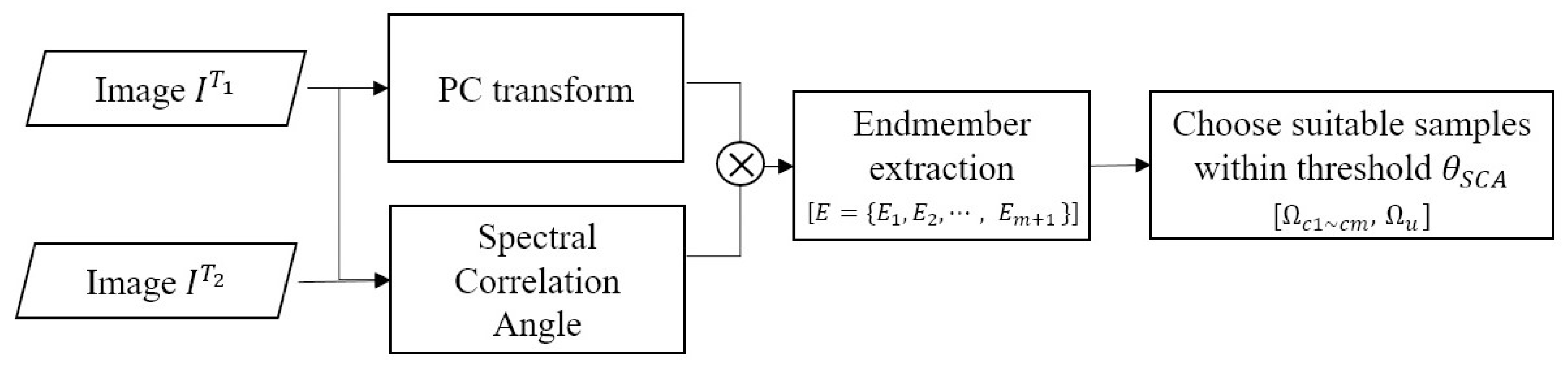
- Generating samples for network training using PCA and similarity measures. To identify multiple changes, a difference image (DI) was produced using PCA and the spectral similarity measure. The PCs and SCA were calculated using multi-temporal images and fused to form the DI. To select training samples of each class, the endmembers were extracted as a reference spectrum of each class. Finally, the pixels in which spectral angle was lower than the threshold were assigned to each endmember class. The samples were then selected randomly, and 3D image patches centered at each selected sample were fed into the Re3FCN network.
- (2)
- Training the Re3FCN and producing the CD map. The 3D patches obtained from each image passed through the 3D convolutional layer to extract spectral and spatial information, whereupon the spectral–spatial feature maps were fed into the ConvLSTM layer. In this phase, the temporal information between two images was reflected. The output of the ConvLSTM layer was fed into the prediction layer to generate the score map. The number of final feature maps equaled the number of classes. Finally, the pixels were classified to the final classes according to the score map.
2.1. Sample Generation
Let and be two HSIs acquired over the same location at different times and , respectively. The size of each image is (, where and are the columns and rows of the image, respectively, and L is the number of spectral bands. Figure 1 shows the flow of generating samples for network training. Generally, PCA can be applied in two ways to detect changes in multi-temporal images [42]. First approach involves directly comparing independently obtained PCs from different images with other CD methods, such as image differencing and regression analysis. The second approach involves combining multi-temporal images with bands into one image with () bands; then, the stacked image is transformed to () PCs.
The stacked image can be simplified as follows. and can be expressed in a matrix as follows:
where and are the number of bands and and represent of the number of pixels of and , respectively. If and have the same size, = and = . Considering each band as a vector, the stacked image can be simply defined as follows:
In , two images in an unchanged area are relatively correlated and two images in a changed area are relatively uncorrelated [42]. The first PC represented the maximum variance of the multi-temporal images and the second PC represented the largest variance not explained by the first PC. In this way, the first component represented unchanged information between two images, and the subsequent PCs were related to the change information. However, because PCA is a scene-dependent technique, the changed portion of the whole scene affected the results of newly obtained PCs, as described in Reference [43]. Therefore, the CD was achieved by analyzing the relative contribution of each input band of the PCs. The contributions of the original input bands and the PCs could be determined from the loadings, which were calculated from the eigenvectors and eigenvalues obtained from the PCA. The eigenvalues represented the percentage of the total variance explained by each PC, and the eigenvectors provided the orientations of the PC axes in the p-dimensional space, where p was the number of extracted PCs. By considering the eigenvalues and loadings, the optimal PCs were selected that distinguished the changes. The loading equation was
Although the optimal PCs show the changed and unchanged pixels; some pixels are not distinguished by the PCs. To discriminate between the changed and unchanged pixels, the optimal PCs and spectral similarity values are combined. A measurement of spectral similarity identifies the finer spectral differences between the two images, which are the differences that the PCs cannot detect. Therefore, combining the PCs and spectral similarity values increases the possibility of discriminating multivariate changes. Our study used the SCA, which reflected the level of the linear correlation between two spectral vectors. The SCA is an angle of the SCM and has been used widely to detect spectral changes because it is less affected by illumination and shadows, due to the relative insensitivity gain and bias factors [44]. The SCM and SCA are calculated as follows:
where and are the mean values of the vectors of and , respectively. The SCA varies between zero and radians. The DI (i.e., the combination of the PCs and SCA) is generated by
where and are the i-th band and the selected PC, respectively. The DI is the weighted PCs. After generating the DI, we used iterative error analysis (IEA), as in Reference [45], to extract the endmembers. The endmembers represented spectral signatures of the pure materials in the scene. Thus, the endmembers, obtained from the DI, represented the unique spectra of various changed and unchanged classes. IEA is a popular endmember extraction method that extracts endmembers one by one in sequential steps. As an input parameter, IEA requires the number of endmembers to be extracted. In the CD analysis, the number of extracted endmembers was taken as the number of total classes (m + 1), which included the changed classes = {, , , and the unchanged class . The extracted endmembers contained the representative spectral information of each class.
Finally, the pixels were clustered to each endmember class using the spectral similarity values. The SCA was calculated between all the pixels and endmembers. The pixels with a smaller SCA matched to each endmember spectrum. However, the pixels with a bigger SCA than the maximum angle threshold were not classified; rather they were assigned to the background class . Pixels were extracted randomly from and as training samples; whilst no pixels were taken from . The 3D image patches centered at these pixels were fed into the network.
2.2. Training Re3FCN and Producing CD Map
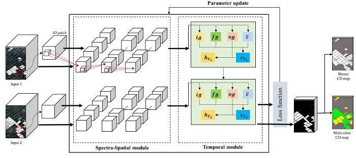
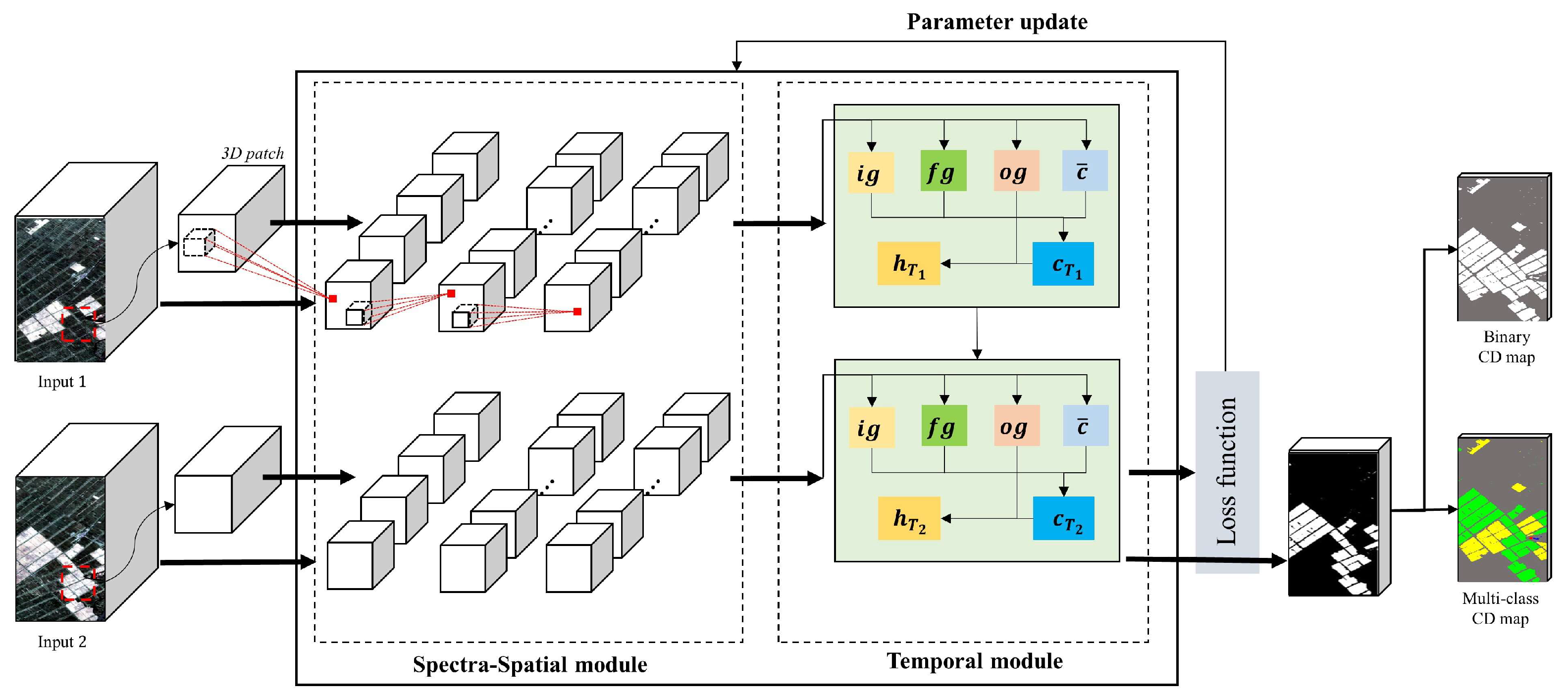
The Re3FCN is based on FCN architecture that includes 3D convolutional layers and the ConvLSTM. Figure 2 shows the architecture of the Re3FCN. Rather than using a fully connected layer, the network uses a convolutional layer at its end. The Re3FCN has two main modules, namely the spectral–spatial module and the temporal module, trained in an end-to-end manner and it preserves the spatial structure during the learning process. A simple network with low complexity is suitable for hyperspectral CD tasks. This is because small patches are used as input, which naturally reduces the depth of the network, and the predicted classes are relatively simple in comparison to other classification tasks. For example, ImageNet classification has 1000 categories and the PASCAL VOC classification has 20 classes [31].
2.2.1. Spectral-Spatial Module with 3D Convolutional Layers
3D patches were selected randomly from and equivalently from . Let and be 3D patches taken from the same location in and , respectively. and were fed separately into the spectral–spatial module of each branch. The spectral–spatial module in the Re3FCN had three 3D convolutional layers and batch normalization (BatchNorm) layers. The BatchNorm layer was placed after the 3D convolutional layer. The BatchNorm layers facilitate higher learning rates and reduce the dependency on initialization, thereby enabling more stable and faster training [46].
Many studies have used 2D CNNs to predict spatial distributions for HSIs, because 2D convolutional layers exploit any local spatial correlation in the images that enforce a local connectivity pattern between the neurons of adjacent layers [47]. However, to effectively apply 2D CNN for hyperspectral feature learning, pre-processing such as PCA for dimension reduction, and post-processing such as the fusion of spectral information, should be conducted [10,47,48]. The processing is achieved because performing 2D convolution on all image bands separately requires many learnable parameters when applied to an HSI with hundreds of bands. This inevitably leads to overfitting, which is a burdensome calculation process. Moreover, a 2D convolution does not conduct inter-band calculation; therefore, the spectral relation between the bands is not considered. 2D convolution can be expressed as:
where is the pixel value at position on the j-th feature map in layer l, where the current operation is located. is the activation function, and b is a bias. is the weight value at position in the n-th shared kernel. N is the number of feature maps in the -th layer.
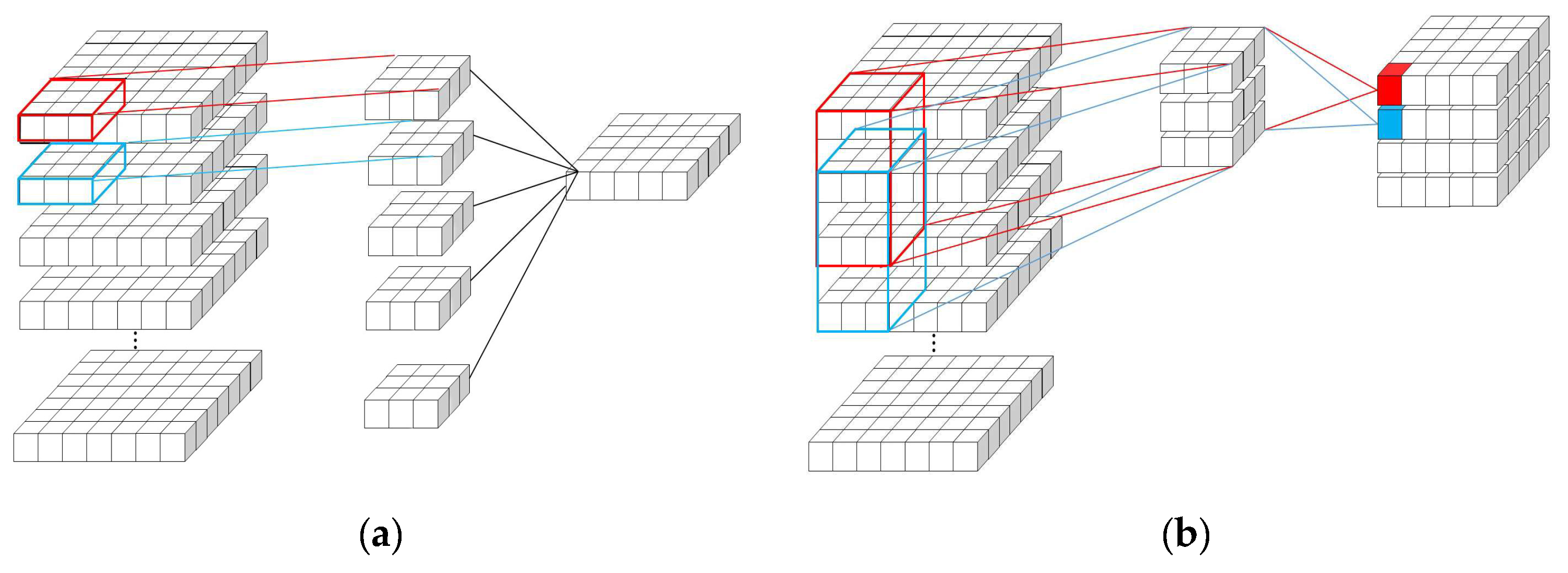
To solve the limitation of 2D convolution, 3D convolution has been introduced for HSI processing and many studies have shown the effectiveness of 3D convolution for HSI classification [37,49]. 3D convolution can extract both spatial and spectral features simultaneously using a 3D kernel. 3D convolution is calculated as:
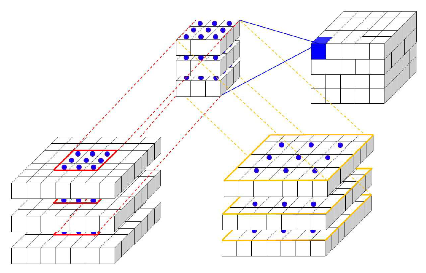
where is the pixel value at position in the j-th 3D feature cube and in the l-th layer. R is the spectral dimension of the 3D kernel, and is the weight value at position connected to the n-th feature in the -th layer. Figure 3 shows the difference between 2D convolution and 3D convolution. Compared to 2D convolution, 3D convolution can obtain spectral and spatial tensors.
Generally, in a deep-learning network, pooling layers are used to reduce the computational cost and to prevent overfitting. However, pooling layers lead to a serious loss of spatial dimension of the feature maps. In this case, the Re3FCN used dilated convolution [50], instead of traditional convolution and pooling. Dilated convolution [51] defines the spacing filled with zero between the original kernel values, which allows the size of the receptive field to be extended without losing spatial resolution. Figure 4 shows dilated convolutions with different dilation rates. The operation of 3D convolution with a dilation rate is formulated as:
2.2.2. Temporal Module with Convolutional LSTM
Feedforward networks, such as CNNs, assume that all inputs are independent. When extracting features, a CNN does not consider the temporal relationship between two inputs. However, in the CD tasks, many dependent portions between the time-series data were available because generally, changes occurred as a minor portion in the entire study site. Thus, it was helpful to derive timely information for the CD. Unlike CNNs, RNNs are designed to deal with dependent sequential inputs, used to solve sequential learning problems. An RNN can explore the temporal dependency of multi-temporal images by connecting previous information to the present task using recurrent hidden states.
To solve this problem, the LSTM was proposed as described in [52], which is an RNN architecture that can remember values over arbitrary intervals using a memory cell at time step t. The LSTM has three gates, namely the input gate , the output gate , and the forget gate , each of which has a learnable weight. is the gate for forgetting the previous information. The output range of the sigmoid function is 0–1: if = 0, the previous state information is forgotten; if = 1, the previous state information is memorized. is the gate for remembering the current information. The cell states are regulated, where they are deleted or added with information through the gates.
Let and be the spectral-spatial feature maps obtained from and , respectively. The simplest LSTM can be expressed as in Reference [32]
Here, “” is the matrix multiplication operator. The weight matrix subscripts have specific meaning. For example, and are the weight matrices between and , the bias of , respectively.
is the candidate cell value and constructs a new candidate value with , which is added to the memory cell to influence the next state. Finally, output is determined by multiplying tanh () and [Equations (14) and (15)], where “” is the element-wise multiplication.
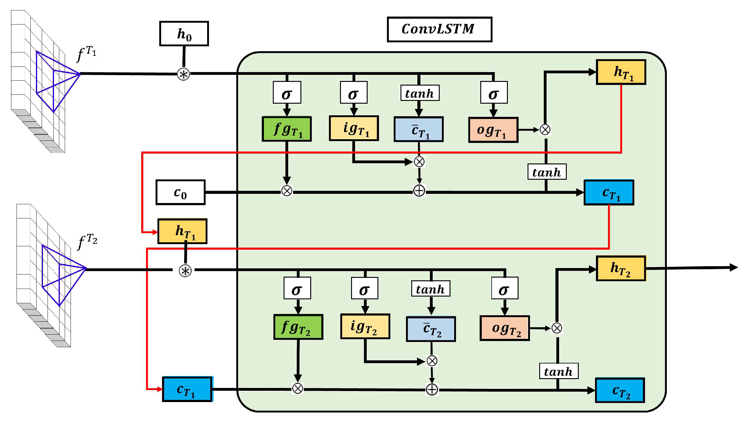
Although the conventional LSTM deals with temporal data, its architecture is not suitable for images and feature maps because (i) the size of the weight matrix increases the computational cost and (ii) spatial connectivity is ignored [36]. ConvLSTM is a modification of the conventional LSTM through replacing the matrix multiplication operators with the convolution operators. ConvLSTM operates as Equations (17)–(20), which is the modification of Equations (11)–(16), wherein the matrix multiplication operators are replaced by convolution operators. Its structure is shown in Figure 5.
Here, “” is a convolutional operator. The three gates of ConvLSTM have 3D tensors. ConvLSTM determines the future state of a cell in the pixel based on the input and past state of its adjacent region using a convolutional operator [36].
After and are fed into each temporal module of the , branch, ConvLSTM will output a sequence . Usually, before the first input is fed into the ConvLSTM, and are initialized to zero, revealing the ignorance about future information. Moreover, and have the same size as the inputs of zero padding that were used. The Re3FCN has one more convolutional layer called the prediction layer and an activation function layer, such as softmax and sigmoid, to generate heat maps. Herein, only the ConvLSTM output is fed into the final prediction layer. Then, the sigmoid layer is used for binary CD and the softmax layer is used for multi-class CD. The cross entropy (CE) loss function is used for parameter updates. The CE can be computed as follows [47]:
where W and b are the parameter sets of weights and bias, respectively. is the predicted class label, and is the ground-truth label for a given sample. K is the number of classes, and l is the total number of training patches. The stochastic gradient descent algorithm with momentum is used for parameter updates. The t-th parameters are updated as follows:
where is the learning rate for step length control, which is set as 0.001 in our experiments, and the gradients are calculated using back-propagation as described in Reference [53].
2.2.3. Quality Evaluation
To evaluate the proposed method, we calculated the overall accuracy (OA), the Kappa coefficient, and the producer accuracy (PA) by class. The OA was the number of correctly classified pixels divided by a total number of sampled pixels. The Kappa coefficient measured how closely the images were classified by the specific classifier with the ground-truth map. In other words, Kappa was a value that compared an observed accuracy with an expected accuracy. For the Kappa coefficient, >0.8 represents a strong agreement between the classification result and the ground truth, 0.6–0.8 represents good accuracy, 0.4–0.6 represents moderate accuracy, and <0.4 represents poor accuracy as outlined in Reference [54]. The PA was the measure of the omission error, which represented the pixels belonging to one class that were incorrectly included in other classes.
Herein, we compared the accuracy of the Re3FCN with several other methods, namely the CVA, IR-MAD, PCA-SCA, support vector machine (SVM) [55], FCN, and the combination of 2DCNN-fully connected LSTM (2DCNN-LSTM). CVA and IR-MAD are effective unsupervised CD methods that have been used in many binary CD studies [12,31,32]. PCA-SCA is the fusion of PCA and SCA. Herein, we used PCA-SCA for sample generation to extract endmembers and for multi-class CD, because it can provide multiple changes through fusion techniques. SVM is a supervised classifier that finds a hyperplane in an N (the number of features) dimensional space to classify the data. In this paper, the SVM with RBF kernel was used.
k-means clustering was used to select thresholds automatically for unsupervised methods, such as the CVA and IR-MAD. PCA-SCA classified the pixels according to the SCA values with endmembers. To compare our model with the other deep-learning architectures, we used FCN and 2DCNN-LSTM for both the binary and multi-CD. The FCN architecture used in the experiment comprised of several convolutional layers with a 2D kernel for feature extraction and pixel labels prediction. The 2DCNN-LSTM has the same structure of that described in Reference [32], and it is mainly composed of three sub-networks such as a 2D convolutional network, a recurrent network, and fully connected layers. The network uses fully connected layers at the end of the structure for predicting labels. As the CVA, IR-MAD, PCA-SCA, SVM, and FCN cannot deal with separated images, we used stacked images as input for these methods, whereas the 2DCNN-LSTM and Re3FCN that received multi-temporal images as input were trained in an end-to-end manner.
3. Dataset
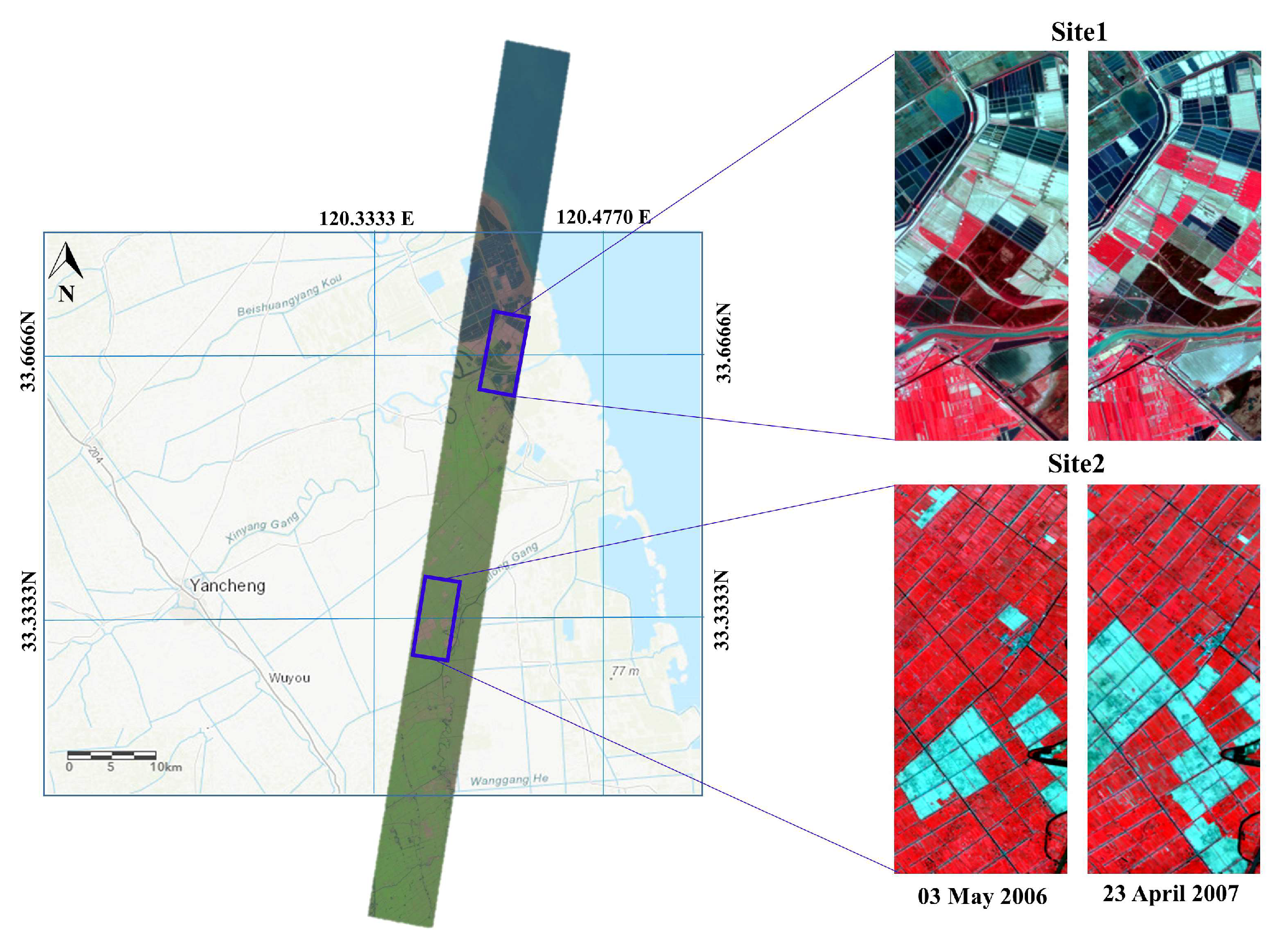
The dataset included two sites of hyperspectral EO-1 Hyperion multi-temporal images obtained from Yancheng in the Jiangsu province of China, which is a wetland agricultural area. The multi-temporal images were acquired on 3 May 2006 ( and on 23 April 2007 ( and the images were registered using geographic map projection WGS-84. The center coordinates of the sites were (33°39’51.85 N, 120°18’16.25 E) and (33°40’49.44 N, 120°30’57.96 E), respectively (Figure 6). The Hyperion spatial resolution was 30 m, and its spectral resolution was 10 nm in 242 bands ranging from 0.400 to 2.500 μm. Subset images with 400145 pixels and 114 spectral bands ranging from 0.5184 to 2.335 μm were used after removing the noise and uncalibrated bands. Pre-processing, such as geometric and radiometric correction was applied to the multi-temporal images before CD.
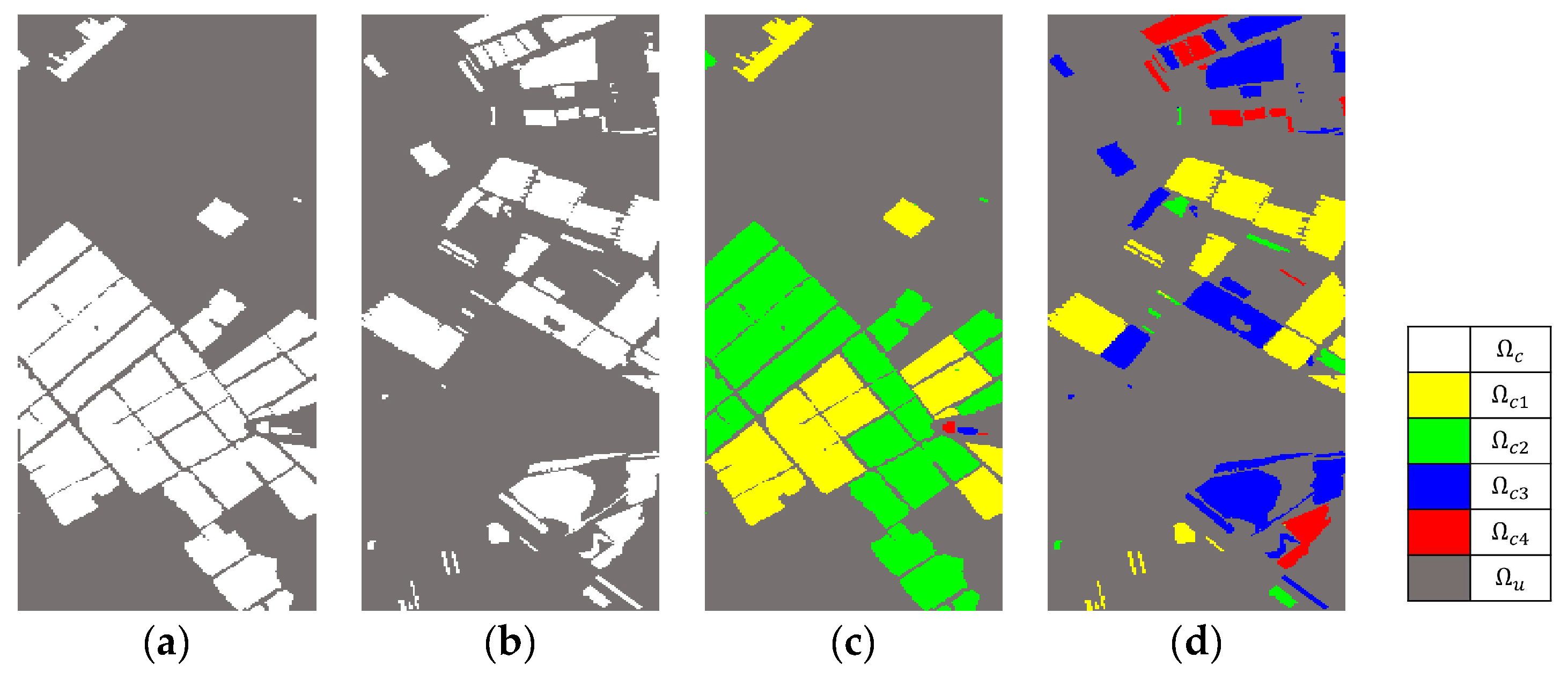
In the dataset, changed and unchanged classes were defined as and , respectively. Binary CD distinguished the pixels of the sites into changed and unchanged classes. Figure 7a,b show the ground-truth maps for the binary CD. To conduct multi-class CD, we divided into depending on the pattern of changes from to . The four major land-cover changes are related to vegetation, bare soil, and water changes [33]. The ground truths with four classes of sites 1 and 2 are shown in Figure 7c,d, respectively. represented changes from bare soil to vegetation, was from vegetation to bare soil, was from bare soil to water, and was from water to bare soil. Site 2 comprised of many wetland areas, covered by water. Therefore, changes in the wetlands were considered as water changes; for example, represented changes from bare soil to wetland, and represented changes from wetland to bare soil.
4. Results
4.1. Sample Generation
4.1.1. PCs for CD
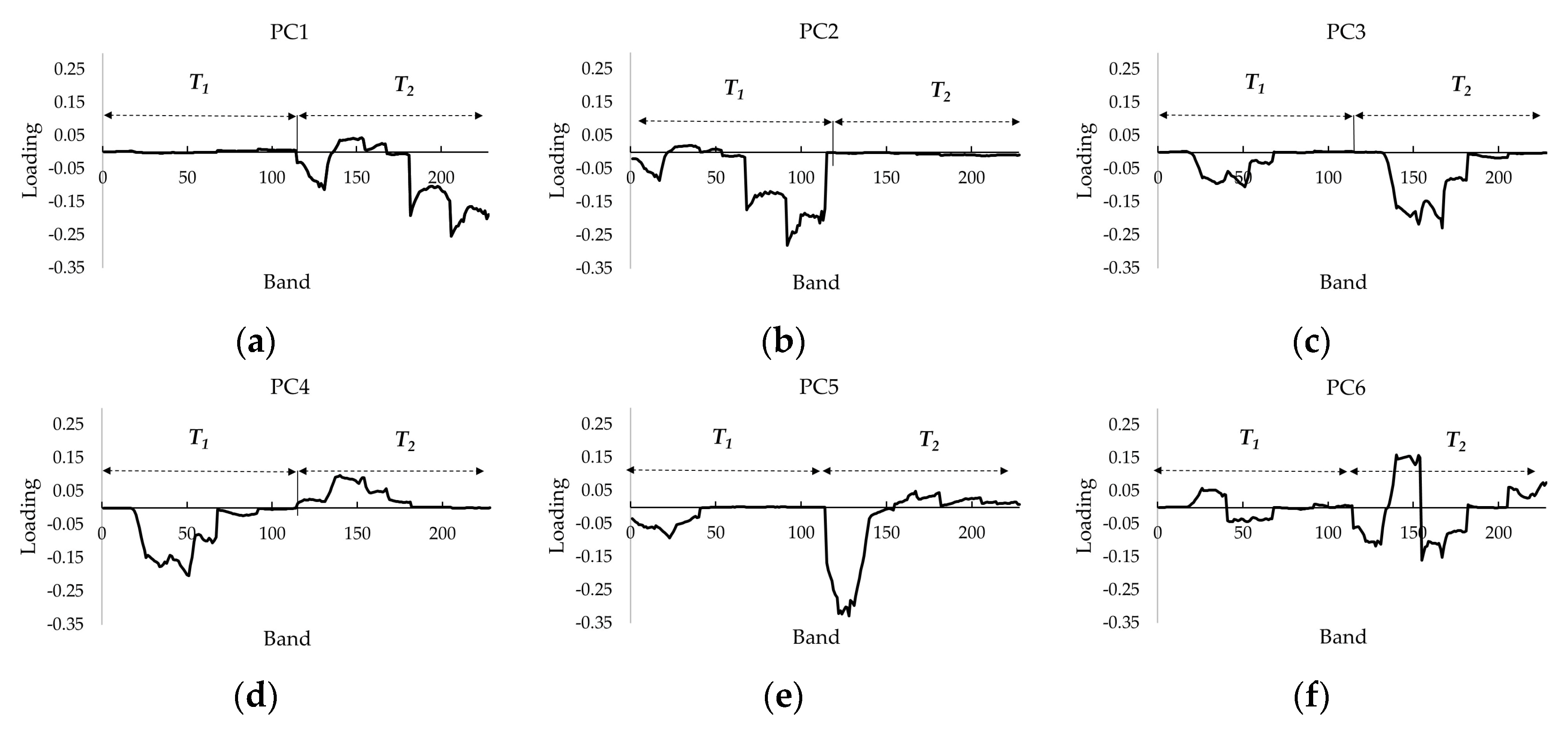
To generate training samples, we applied PCA to the stacked images. The objective of this phase was to transform the multi-temporal images to make the changed and unchanged areas prominent in the scene. Table 1 and Table 2 provide the eigenvalues and cumulative percentage variances for the newly obtained PCs for sites 1 and 2, respectively, and Figure 8 and Figure 9 show the loadings of each PC. By analyzing the eigenvalues and loading factors, we selected those PCs that were most useful for identifying the changed or unchanged areas. In the case of site 1, we extracted PC1–PC6 because they accounted for roughly 99% of the total variance in the staked multi-temporal image. The percentage variance indicates the number variance in the multi-temporal images that is explained by the PC. As PCs with low rank tend to concentrate uncorrelated noise between bands, we extracted the first few PCs. As shown in Figure 8a, PC1 is loaded mainly on the image and has a negative loading in the visible band and a positive loading in the infrared band. This suggested that PC1 was mainly a summary of the vegetation pixels in the image. In contrast with PC1, PC2 was mainly loaded on vegetation pixels in the image (Figure 8b). Given PC1 and PC2 described the vegetation information in each period, it was possible to extract change information using those components. Moreover, PC4 was negatively loaded on and positively loaded on in the red and infrared bands. Thus, PC4 could be used to measure the changes in those pixels that have contrast reflectance between two periods. In the same way, we selected PC5 and PC6 as the final optimal PCs for CD. However, PC3 had negative loadings in the visible and infrared bands on both the and images. This meant that PC3 represented those pixels that had low reflectance in the visible and infrared bands in both scenes that were not suitable for analyzing changes in land cover.
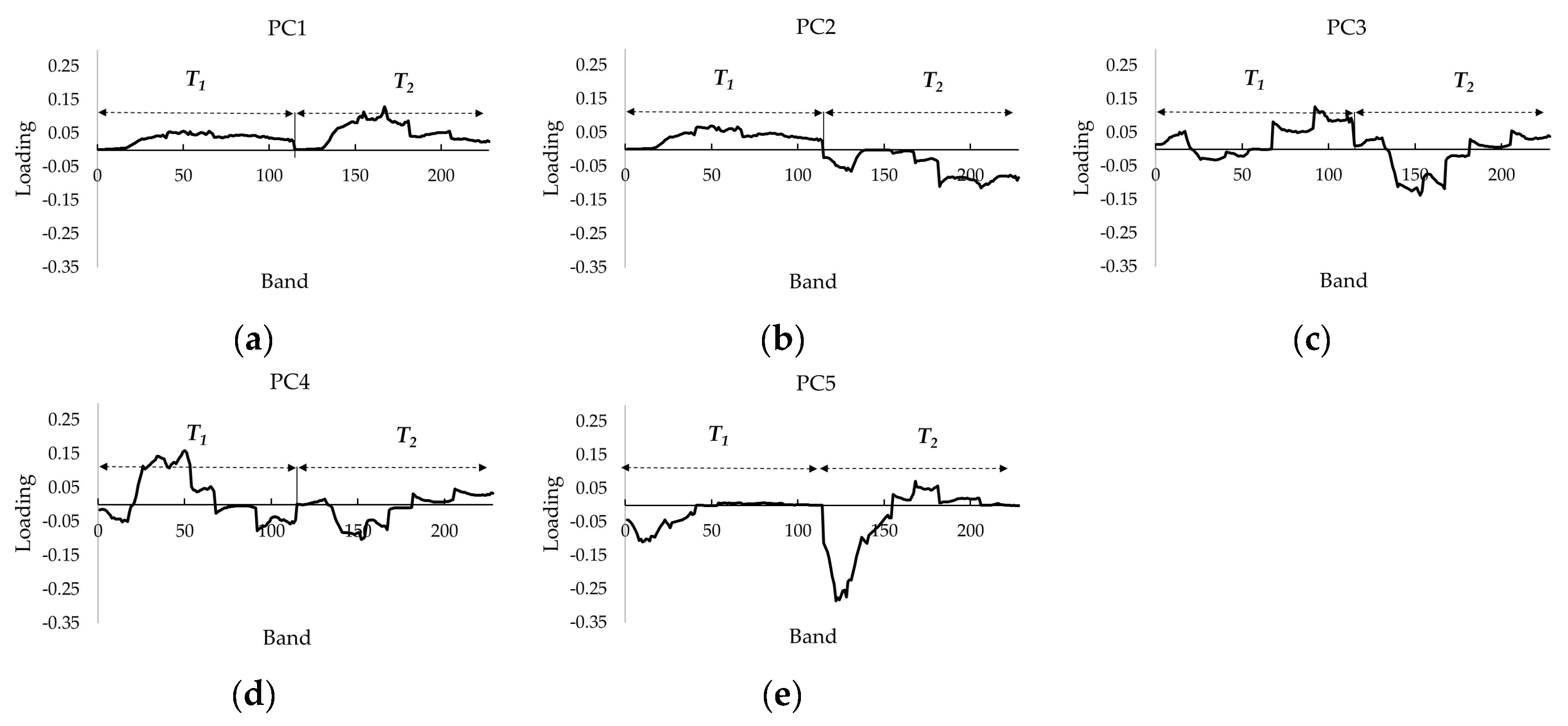
In the same way, we selected PC1–PC5 obtained from site 2 because they accounted for roughly 99% of the total variance in the multi-temporal images. We selected PC2, PC4, and PC5 as the final PCs as they represented change information; for example, PC2 was positively loaded in the image, but negatively loaded in the image. Therefore, PC2 could be used to measure brightness changes in the pixel reflectance. In contrast, PC1 was loaded positively and evenly in all bands in both the and images. Thus, the pixels had similar reflectance patterns in both times. PC3 was excluded from the optical PCs because it possibly represented pixels with similar reflectance patterns.
4.1.2. Clustering Pixels by SCA with Endmembers
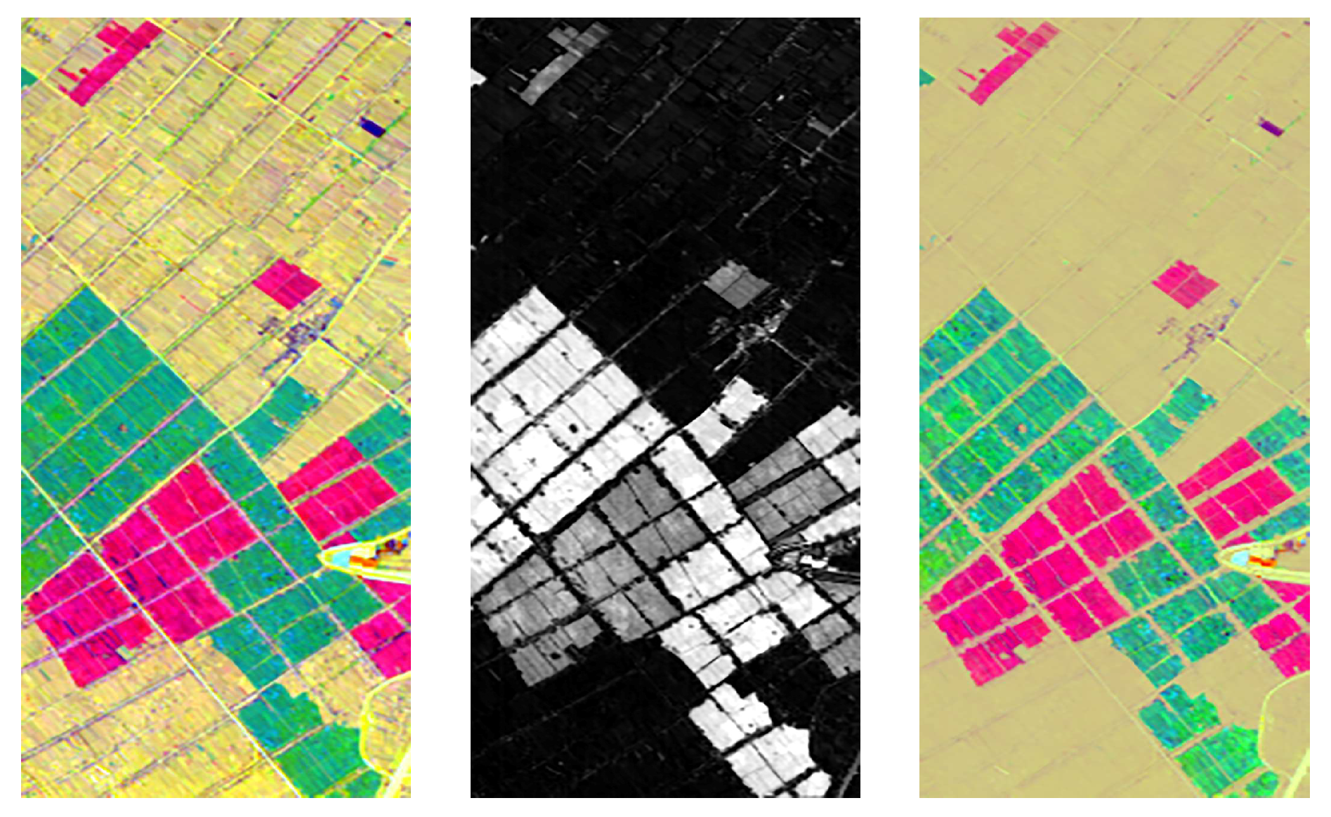
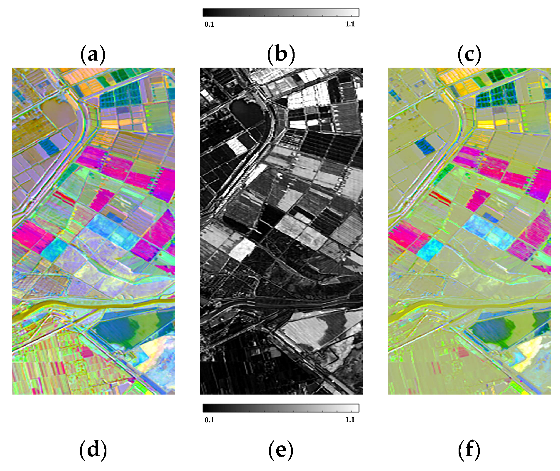
After the final PCs were selected for CD, the PCs were fused to SCA values, which were calculated between multi-temporal images. Figure 10 shows the color composites of the optimal PCs, SCA value maps, and the results of the fusion of PCs and SCA for sites 1 and 2. In the fused images, the changed and unchanged areas were more clearly distinguished than the original color composite of the PCs. This was because a large value of the SCA was multiplied on a pixel, where the spectral difference was great (assumed as the changed area), and a small value close to zero was multiplied on a pixel, where the spectral difference in the multi-temporal image was small (assumed as the unchanged area). This assisted in distinguishing and highlighting the unchanged/changed areas and the multiple changes in the images.
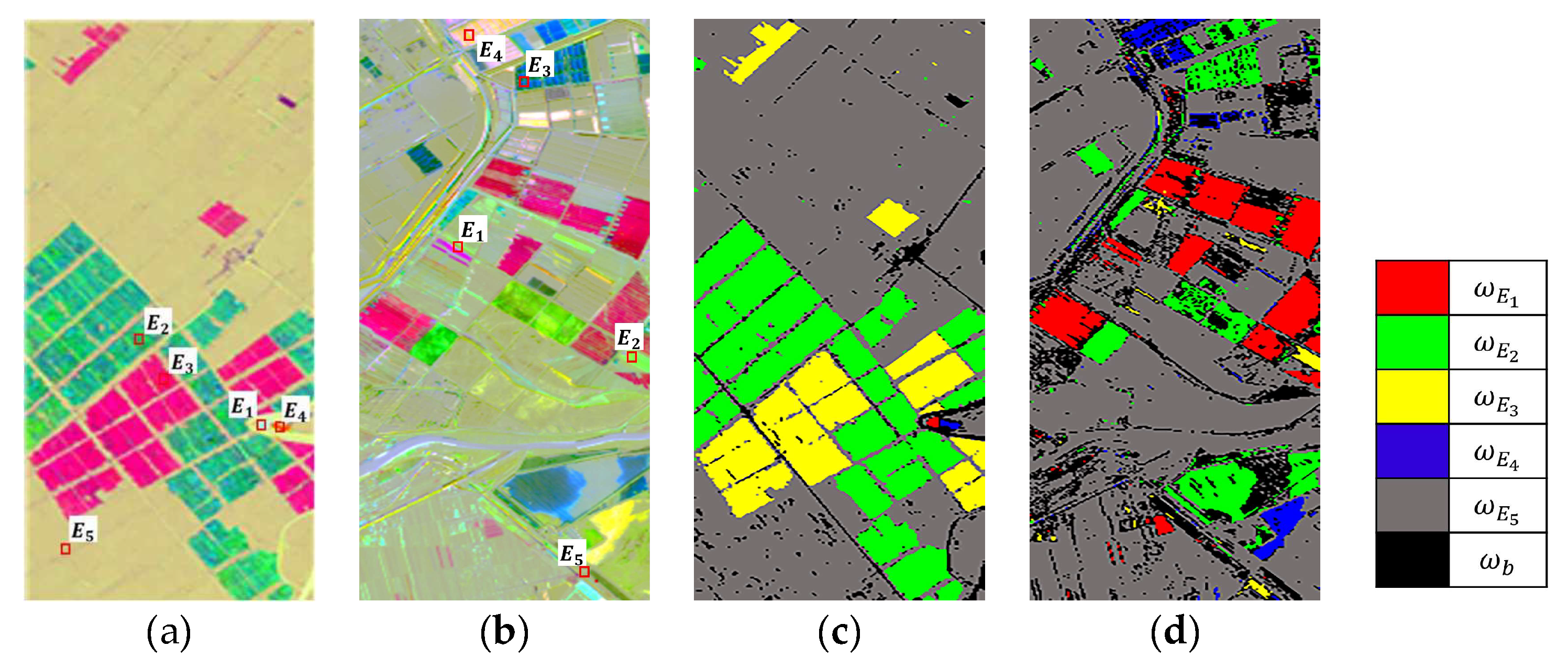
The endmember set , , ] was extracted using IEA, and the number of endmembers was set to five, which was the total number m of changed classes plus the one unchanged class. Since the endmembers represented pure pixels that had unique spectral values in the scene, the distinguished features in the fusion images were the extracted endmembers. The locations of the endmembers are shown in Figure 11a,b. were extracted from the specific changed or unchanged classes.
Finally, the training samples were generated by assigning the pixels to specific endmember classes with the SCA threshold values, which was calculated between and all the pixels (Figure 11c,d). For example, was the class of , and those pixels with SCA values lower than the threshold value of were assigned to class . Herein, the threshold was set to 0.05, which was determined experimentally. If the threshold value was set too high, then the pixels were more likely to be classified incorrectly. If the value was set too low, then the number of training samples was insufficient. Therefore, an appropriate value must be set, revealing that a value in the range 0.05–0.1 is suitable. Since the pixels were assigned by the threshold value, some of the pixels that did not have SCA values within the threshold for any were not classified. This class was labeled and the pixels in this class were not used in the samples for network training. The samples were divided into training and testing samples. Table 3 provides the numbers of ground truths and the training/testing samples for binary and multi-class CD. Of all the samples, 70% were used for training, and 30% were used for testing. For site 1, and (which represent and respectively) contributed relatively few samples, and for site 2 contributed a larger portion than that of site 1. Table 4 gives the PA of except . The samples were extracted with high accuracy. The OA of for site 1 was higher than that of site 2. The reason for the difference was that as site 2 contained many materials with similar spectral properties (e.g., wetlands over vegetation, which exhibited both vegetation and water characteristics), the pixels could be misclassified into different endmembers.
4.2. Change Detection Results and Discussion
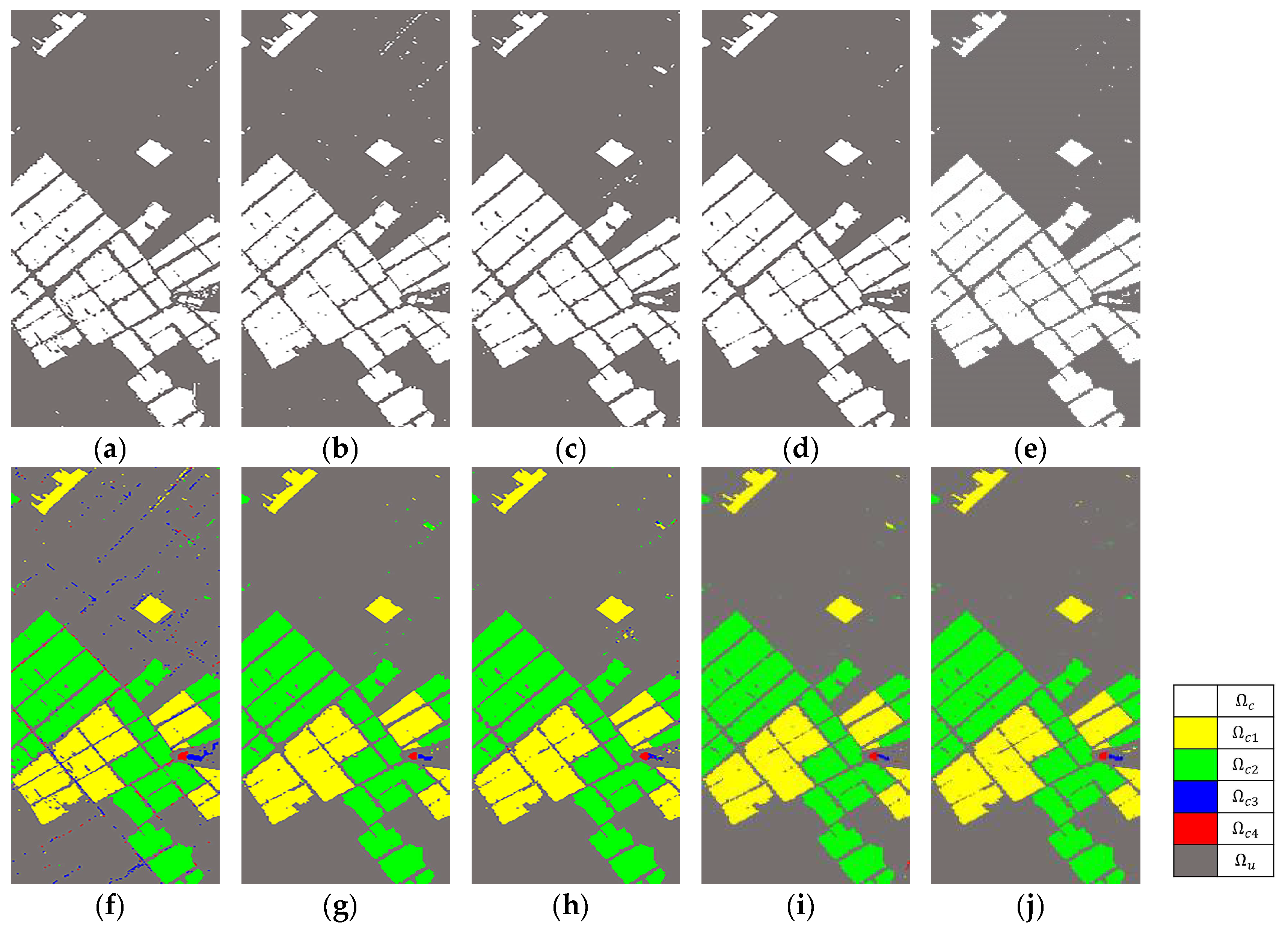
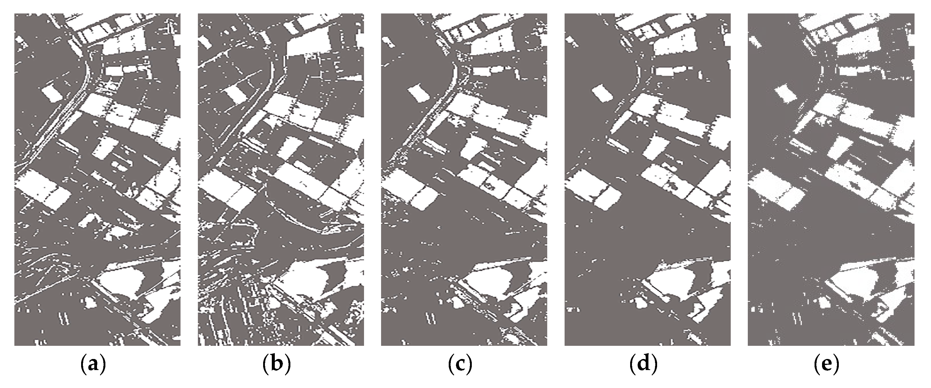
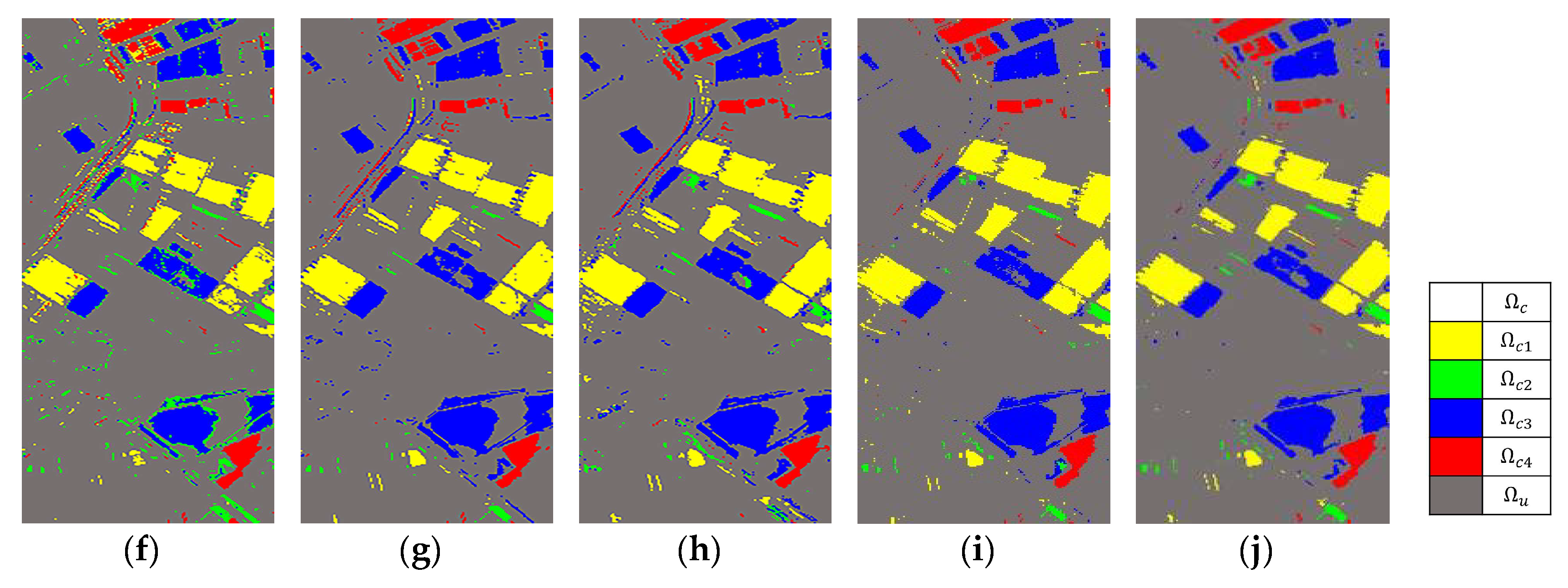
Figure 12 and Figure 13 show the binary and multi-class CD maps obtained from the Re3FCN and other methods. The OA, Kappa coefficient, and accuracy of all the class methods on the binary and multi-class CD are given in Table 5 and Table 6. To compare the CD ability in samples where no training samples were extracted, the accuracies in class were calculated. Compared to site 1, site 2 had lower OAs and Kappa coefficients for all the methods. This seemed affected by the sample accuracies. The sample classes of site 1 were more accurate than those of site 2. Moreover, most errors were identified in the class pixels, (which had no sample data), because site 2 had a higher portion of pixels as compared with site 1, the OA and Kappa values were lower in site 2 as compared to site 1. The results showed that the sampling error in the sample-generation step could affect the accuracy of the entire CD results. Nevertheless, the CD results on pixels can provide useful information for confirming the likelihood of CD in the absence of reference data.
Although classical unsupervised CD methods, such as CVA and IR-MAD with k-means clustering and PCA-SCA achieved good performance compared to the SVM and other deep-learning methods, errors occured in class and at the edges of the classes. For example, CVA and IR-MAD had the lowest OA and Kappa coefficient in site 1 and site 2, respectively. Moreover, PCA-SCA showed relatively poor CD results as compared to those of the other methods. Many errors occured at the edges of the objects. This was because the PCA-SCA considers only spectral values when classifying the pixels of spectrally similar materials; for example, shadows in the object edge line and water that have low reflectance can be misclassified.
SVM and the deep-learning methods outperformed the classical methods in terms of the OA and Kappa coefficient in both site 1 and site 2, including the pixels in . However, the FCN and SVM need specific operation like image stacking before the CD. Moreover, 2DCNN-LSTM and Re3FCN achieved better performance than that of the FCN with a 2D kernel and the SVM. For example, the OA and Kappa coefficient of the FCN in site 2 for binary CD were 0.938 and 0.822, respectively. The respective improvements in the OA and Kappa coefficient were 1.3% and 0.030 achieved by the 2DCNN-LSTM and 3.1% and 0.089 achieved by the Re3FCN. Furthermore, for a multi-class CD in site 2, the OA and Kappa coefficient of the SVM were 0.945 and 0.875, respectively, but the 2DCNN-LSTM delivered improved values of 0.951 (OA) and 0.880 (Kappa coefficient); and the Re3FCN delivered improved values of 0.962 (OA) and 0.895 (Kappa coefficient). The results showed the possibility that using recurrent convolutional networks could be effective for hyperspectral CD.
Furthermore, comparing the Re3FCN and the 2DCNN-LSTM, although both methods showed good performance and had similar accuracies, the results showed that the Re3FCN had the most stable and best performance in both site 1 and site 2. In particular, the Re3FCN was efficient at detecting binary and multi-class changes and it achieved the highest accuracies in class in all the CD experiments. For example, the OA and Kappa coefficient of the 2DCNN-LSTM and the Re3FCN in site 1, in terms of binary CD, had similar OA and Kappa coefficients such as 0.977 (OA), 0.949 (Kappa coefficient), and 0.981 (OA), 0.958 (Kappa coefficient). However, the accuracies on of the Re3FCN (0.928) was higher than the 2DCNN-LSTM (0.917). Moreover, the accuracies in the multi-class CD in site 2, Re3FCN, had a higher OA (0.899) on the pixels included in than 2DCNN-LSTM OA (0.861). The results showed that the Re3FCN could learn change rules from existing data and could be applied effectively to pixels without reference data. The present CD experiment confirmed that using a 3D convolution and ConvLSTM allowed a spectral–spatial–temporal change detector to be constructed.
5. Conclusions
In this study, we proposed a novel sample generation and a CD network, called the Re3FCN. This method merged the advantages of both a 3D FCN and a convolutional LSTM. The PCA and SCA were combined to generate reliable samples with high accuracy, and the training samples were determined based on the SCA value for each endmember. This method assists in conducting CD in cases where there are is reference or training data, such as in unsupervised CD. Furthermore, the Re3FCN (i) can extract spectral–spatial–temporal information between multi-temporal images, (ii) is effective in detecting binary and multi-class changes whilst maintaining the spatial structural inputs by replacing fully connected layers with convolutional layers, and (ii) can be trained in an end-to-end manner. The CD results were compared with those of the CVA, IR-MAD, PCA-SCA, SVM, FCN, and 2DCNN-LSTM. The Re3FCN outperformed them in both the binary and multi-class CD. Particularly, the Re3FCN was effective in detecting changes in areas from which no training samples had been extracted.
However, several problems in the CD method were identified; for example, the errors associated with sample generation can affect the final CD. To solve these problems, we improved the accuracy of the training-sample generation and conducted additional experiments to confirm the ability to learn changed rules from multi-temporal images obtained from different sensors.
Author Contributions
Conceptualization, all authors; Methodology, A.S. and J.C.; Software, A.S. and J.C.; Validation Y.H.; Formal analysis, Y.K., J.C., and Y.H.; Data curation, J.C. and Y.H.; Writing (original draft preparation), A.S.; Writing (review and editing), J.C. and Y.H.; Funding acquisition, Y.K.; Supervision, Y.K.; Project administration, Y.K. and J.C.
Funding
This research was supported by the National Research Foundation of Korea (NRF) funded by the Korean government (MSIT) (grant no. NRF-2016R1A2B4016301) and by a grant (18SIUE-B148326-01) from Satellite Information Utilization Center Establishment Program by Ministry of Land, Infrastructure and Transport of Korean government.
Conflicts of Interest
The authors declare no conflict of interest.
References
- Adão, T.; Hruška, J.; Pádua, L.; Bessa, J.; Peres, E.; Morais, R.; Sousa, J.J. Hyperspectral imaging: A review on UAV-based sensors, data processing and applications for agriculture and forestry. Remote Sens. 2017, 9, 1110. [Google Scholar] [CrossRef]
- Yang, X.; Ye, Y.; Li, X.; Lau, R.Y.K.; Zhang, X.; Huang, X. Hyperspectral image classification with deep learning models. IEEE Trans. Geosci. Remote Sens. 2018, 56, 5408–5423. [Google Scholar] [CrossRef]
- Yuan, Y.; LV, H.; LU, X. Semi-supervised change detection method for multi-temporal hyperspectral images. Neurocomputing 2015, 148, 363–375. [Google Scholar] [CrossRef]
- Singh, A. Review article digital change detection techniques using remotely-sensed data. Int. J. Remote Sens. 1989, 10, 989–1003. [Google Scholar] [CrossRef]
- Rumpf, T.; Mahlein, A.K.; Steiner, U.; Oerke, E.C.; Dehne, H.W.; Plümer, L. Early detection and classification of plant diseases with support vector machines based on hyperspectral reflectance. Comput. Electron. Agric. 2010, 74, 91–99. [Google Scholar] [CrossRef]
- Pu, R.; Gong, P.; Tian, Y.; Miao, X.; Carruthers, R.I.; Anderson, G.L. Invasive species change detection using artificial neural networks and CASI hyperspectral imagery. Environ. Monit. Assess. 2008, 140, 15–32. [Google Scholar] [CrossRef] [PubMed]
- Khan, M.J.; Khan, H.S.; Yousaf, A.; Khurshid, K.; Abbas, A.A. Modern trends in hyperspectral image analysis: A Review. IEEE Access 2018, 6, 14118–14129. [Google Scholar] [CrossRef]
- Khanday, W.A.; Kumar, K. Change detection in hyper spectral images. Asian J. Technol. Manag. Res. 2016, 6, 54–60. [Google Scholar]
- Liu, S. Advanced Techniques for Automatic Change Detection in Multitemporal Hyperspectral Images. Ph.D. Thesis, University of Trento, Trento, Italy, 2015. [Google Scholar]
- Wang, Q.; Yuan, Z.; Du, Q.; Li, X. GETNET: A general end-to-end 2-D CNN for hyperspectral image change detection. IEEE Trans. Geosci. Remote Sens. 2018, 99, 1–11. [Google Scholar] [CrossRef]
- Yu, L.; Xie, J.; Chen, S.; Zhu, L. Generating labeled samples for hyperspectral image classification using correlation of spectral bands. Front. Comput. Sci. 2016, 10, 292–301. [Google Scholar] [CrossRef]
- Xiaolu, S.; Bo, C. Change detection using change vector analysis from Landsat TM images in Wuhan. Procedia Environ. Sci. 2011, 11, 238–244. [Google Scholar] [CrossRef]
- Liu, S.; Bruzzone, L.; Bovolo, F.; Du, P. A novel sequential spectral change vector analysis for representing and detecting multiple changes in hyperspectral images. In Proceedings of the 2014 IEEE International Geoscience and Remote Sensing Symposium, Quebec City, QC, Canada, 13–18 July 2014; pp. 4656–4659. [Google Scholar]
- Singh, S.; Talwar, R. A comparative study on change vector analysis based change detection techniques. Sadhana 2014, 39, 1311–1331. [Google Scholar] [CrossRef]
- Hansanlou, M.; Seydi, S.T. Hyperspectral change detection: An experimental comparative study. Int. J. Remote Sens. 2018, 1–55. [Google Scholar] [CrossRef]
- Ortiz-Rivera, V.; Vélez-Reyes, M.; Roysam, B. Change detection in hyperspectral imagery using temporal principal components. In Proceedings of the SPIE 2006 Algorithms and Technologies for Multispectral, Hyperspectral, Ultraspectral Imagery XII, Orlando, FL, USA, 8 May 2006; p. 623312. [Google Scholar]
- Nielsen, A.A.; Conradsen, K.; Simpson, J.J. Multivariate alteration detection (MAD) and MAF postprocessing in multispectral, bitemporal image data: New approaches to change detection studies. Remote Sens. Environ. 1998, 64, 1–19. [Google Scholar] [CrossRef]
- Nielsen, A.A. The regularized iteratively reweighted MAD method for change detection in multi-and hyperspectral data. IEEE Trans. Image Process. 2007, 16, 463–478. [Google Scholar] [CrossRef] [PubMed]
- Danielsson, P.E. Euclidean distance mapping. Comput. Gr. Image Process. 1980, 14, 227–248. [Google Scholar] [CrossRef] [Green Version]
- Kruse, F.A.; Lefkoff, A.B.; Boardman, J.W.; Heidebrecht, K.B.; Shaprio, A.T.; Barloon, P.J.; Goetz, A.F.H. The spectral image processing system (SIPS)—Interactive visualization and analysis of imaging spectrometer data. Remote Sens. Environ. 1993, 44, 145–163. [Google Scholar] [CrossRef]
- De Carvalho, O.A.; Meneses, P.R. Spectral correlation mapper (SCM): An improvement on the spectral angle mapper (SAM). In Proceedings of the 9th Airborne Earth Science Workshop, Pasadena, CA, US, 23–25 February 2000. [Google Scholar]
- Chang, C.I. Spectral information divergence for hyperspectral image analysis. In Proceedings of the IEEE International Geoscience and Remote Sensing Symposium (IGARSS 1999), Hamburg, Germany, 28 June–2 July 1999; pp. 509–511. [Google Scholar]
- Wu, C.; Du, B.; Zhang, L. A subspace-based change detection method for hyperspectral images. IEEE J. Sel. Top. Appl. Earth Obs. Remote Sens. 2013, 6, 815–830. [Google Scholar] [CrossRef]
- Shi, A.; Gao, G.; Shen, S. Change detection of bitemporal multispectral images based on FCM and D-S theory. EURASIP J. Adv. Signal Process. 2016, 2016, 96. [Google Scholar] [CrossRef]
- Du, Q. A new method for change analysis of multi-temporal hyperspectral images. In Proceedings of the Workshop on Hyperspectral Image and Signal Processing: Evolution in Remote Sensing (WHISPERS), Shanghai, China, 4–7 June 2012; pp. 1–4. [Google Scholar]
- Han, Y.; Chang, A.; Choi, S.; Park, H.; Choi, J. An Unsupervised algorithm for change detection in hyperspectral remote sensing data using synthetically fused images and derivative spectral profiles. J. Sens. 2017, 2017, 1–14. [Google Scholar] [CrossRef]
- Gao, F.; Liu, X.; Dong, J.; Zhong, G.; Jian, M. Change detection in SAR images based on deep Semi-NMF and SVD networks. Remote Sens. 2017, 9, 435. [Google Scholar] [CrossRef]
- Fu, G.; Liu, C.; Zhou, R.; Sun, T.; Zhang, Q. Classification for high resolution remote sensing imagery using a fully convolutional network. Remote Sens. 2017, 9, 498. [Google Scholar] [CrossRef]
- Atkinson, P.P.; Tantnall, A.R.L. Introduction neural networks in remote sensing. Int. J. Remote Sens. 1997, 18, 699–709. [Google Scholar] [CrossRef]
- Lyu, H.; Lu, H.; Mou, L. Learning a transferable change rule from a recurrent neural network for land cover change detection. Remote Sens. 2016, 8, 506. [Google Scholar] [CrossRef]
- Mou, L.; Bruzzone, L.; Zhu, X.X. Learning spectral-spatial-temporal features via a recurrent convolutional neural network for change detection in multispectral imagery. arXiv, 2018; arXiv:1803.02642. [Google Scholar]
- Zhang, L.; Zhang, L.; Du, B. Deep learning for remote sensing data: A technical tutorial on the state of the art. IEEE Geosci. Remote Sens. Mag. 2016, 4, 22–40. [Google Scholar] [CrossRef]
- Liu, S.; Du, Q.; Tong, X.; Samat, A.; Pan, H.; Ma, X. Band selection-based dimensionality reduction for change detection in multi-temporal Hyperspectral Images. Remote Sens. 2017, 9, 1008. [Google Scholar] [CrossRef]
- Ackley, D.H.; Hinton, G.E.; Sejnowski, T.J. A learning algorithm for Boltzmann machines. Cogn. Sci. 1985, 9, 147–169. [Google Scholar] [CrossRef]
- Bengio, Y.; Lamblin, P.; Popovici, D.; Larochelle, H. Greedy layer-wise training of deep networks. In Proceedings of the Advances in Neural Information Processing Systems, Vancouver, BC, Canada, 4–7 December 2006; pp. 153–160. [Google Scholar]
- Xingjian, S.; Chen, Z.; Wang, H.; Yeung, D.Y.; Wong, W.K.; Woo, W.C. Convolutional LSTM network: A machine learning approach for precipitation nowcasting. Adv. Neural Inf. Process. Syst. 2015, 1, 802–810. [Google Scholar]
- Zhu, X.X.; Tuia, D.; Mou, L.; Xia, G.S.; Zhang, L.; Xu, F.; Fraundorfer, F. Deep learning in remote sensing: A comprehensive review and list of resources. IEEE Geosci. Remote Sens. Mag. 2017, 5, 8–36. [Google Scholar] [CrossRef]
- Valipour, S.; Siam, M.; Jafersand, M.; Ray, N. Recurrent fully convolutional networks for video segmentation. In Proceedings of the 2017 IEEE Winter Conference on Applications of Computer Vision (WACV), Santa Rosa, CA, USA, 24–31 March 2017; pp. 29–36. [Google Scholar]
- Lu, N.; Wu, Y.; Feng, L.; Song, J. Deep Learning for Fall Detection: 3D-CNN Combined with LSTM on Video Kinematic Data. IEEE J. Biomed. Health Inform. 2018, 1–10. [Google Scholar] [CrossRef] [PubMed]
- Zhang, L.; Zhu, G.; Shen, P.; Song, J. Learning spatiotemporal features using 3dcnn and convolutional LSTM for gesture recognition. In Proceedings of the IEEE Conference on Computer Vision and Pattern Recognition, Venice, Italy, 22–29 October 2017; pp. 3120–3128. [Google Scholar]
- Robila, S.A. An analysis of spectral metrics for hyperspectral image processing. In Proceedings of the 2004 IGARSS Geoscience and Remote Sensing Symposium, Anchorage, AK, USA, 20–24 September 2004; pp. 3233–3236. [Google Scholar]
- Deng, J.S.; Wang, K.; Deng, Y.H.; Qi, G.J. PCA-based land-use change detection and analysis using multitemporal and multisensor satellite data. Int. J. Remote Sens. 2008, 29, 4823–4838. [Google Scholar] [CrossRef]
- Fung, T.; Ledrew, E. Application of principal components analysis to change detection. Photogramm. Eng. Remote Sens. 1987, 53, 1649–1658. [Google Scholar]
- Carvalho Júnior, O.A.; Guimarães, R.F.; Gillespie, A.R.; Silva, N.C.; Gomes, R.A. A new approach to change vector analysis using distance and similarity measures. Remote Sens. 2011, 3, 2473–2493. [Google Scholar] [CrossRef]
- Neville, R.A.; Staenz, K.; Szeredi, T.; Lefebvre, J. Automatic endmember extraction from hyperspectral data for mineral exploration. In Proceedings of the 21st Canadian Symposium on remote Sensing, Ottawa, ON, Canada, 21–24 July 1999; pp. 891–897. [Google Scholar]
- Santurkar, S.; Tsipras, D.; Ilyas, A.; Madry, A. How does batch normalization help optimization? (no, it is not about internal covariate shift). arXiv, 2018; arXiv:1805.11604. [Google Scholar]
- Cao, X.; Zhou, F.; Xu, L.; Meng, D.; Xu, Z.; Paisley, J. Hyperspectral image classification with Markov random fields and a convolutional neural network. IEEE Trans. Image Process. 2018, 27, 2354–2367. [Google Scholar] [CrossRef] [PubMed]
- Jiao, L.; Liang, M.; Chen, H.; Yang, S.; Liu, H.; Cao, X. Deep fully convolutional network-based spatial distribution prediction for hyperspectral image classification. IEEE Trans. Geosci. Remote Sens. 2017, 55, 5585–5599. [Google Scholar] [CrossRef]
- Li, Y.; Zhang, H.; Shen, Q. Spectral–spatial classification of hyperspectral imagery with 3D convolutional neural network. Remote Sens. 2017, 9, 67. [Google Scholar] [CrossRef]
- Chen, L.C.; Kokkinos, I.; Murphy, K.; Yuille, A.L. Semantic Image Segmentation with Deep Convolutional Nets and Fully Connected CRFs. In Proceedings of the International Conference on Learning Representations (ICLR), San Diego, CA, USA, 7–9 May 2015. [Google Scholar]
- Yu, F.; Koltun, V. Multi-scale context aggregation by dilated convolutions. In Proceedings of the 2016 International Conference on Learning Representations, San Juan, Puerto Rico, 2–4 May 2016. [Google Scholar]
- Hochreiter, S.; Schmidhuber, J. Long short-term memory. Neural Comput. 1997, 9, 1735–1780. [Google Scholar] [CrossRef] [PubMed]
- Rumelhart, D.E.; Hinton, G.E.; Williams, R.J. Learning Internal Representations by Error Propagation. In Parallel Distributed Processing—Explorations in the Microstructure of Cognition; Rumelhart, D.E., McClelland, J.L., Eds.; The MIT Press: Cambridge, MA, USA, 1986; pp. 318–362. [Google Scholar]
- Landis, J.R.; Koch, G.G. The measurement of observer agreement for categorical data. Biometrics 1977, 33, 159–174. [Google Scholar] [CrossRef] [PubMed]
- Hearst, M.A.; Dumais, S.T.; Osuna, E.; Platt, J.; Scholkopf, B. Support vector machines. IEEE Intell. Syst. Appl. 1998, 13, 18–28. [Google Scholar] [CrossRef]
- ArcGIS Webmap. Available online: https://www.arcgis.com/home/webmap/viewer.html (accessed on 11 October 2018).
- Earth Science Data Archives of U.S. Geological Survey (USGS). Available online: http://earthexplorer.usgs.gov/ (accessed on 11 October 2018).
Figure 1.
Flowchart of sample generation. is the endmember set including endmembers. and represent i-th changed class and unchanged class, respectively.
Figure 1.
Flowchart of sample generation. is the endmember set including endmembers. and represent i-th changed class and unchanged class, respectively.

Figure 2.
Architecture of the proposed change detection (CD) method.

Figure 3.
Illustrations of (a) two-dimensional (2D) and (b) three-dimensional (3D) convolution operation.
Figure 3.
Illustrations of (a) two-dimensional (2D) and (b) three-dimensional (3D) convolution operation.

Figure 4.
Dilated convolution. Red wireframe = dilation rate of (1,1,1); yellow wireframe = dilation rate of (2,2,1). This figure shows that a 3 × 3 × 3 kernel with a dilation rate of (2,2,1) will have a receptive field size equal to that of a 7 × 7 × 3 kernel, without loss of spatial resolution.
Figure 4.
Dilated convolution. Red wireframe = dilation rate of (1,1,1); yellow wireframe = dilation rate of (2,2,1). This figure shows that a 3 × 3 × 3 kernel with a dilation rate of (2,2,1) will have a receptive field size equal to that of a 7 × 7 × 3 kernel, without loss of spatial resolution.

Figure 5.
Structure of the convolutional long short-term memory (LSTM). is a randomly initialized hidden state, and is a memory cell. ,, and are forget gates, input gates, output gates, candidate memory cells, memory cells, and hidden states, respectively, at time t.
Figure 5.
Structure of the convolutional long short-term memory (LSTM). is a randomly initialized hidden state, and is a memory cell. ,, and are forget gates, input gates, output gates, candidate memory cells, memory cells, and hidden states, respectively, at time t.

Figure 6.
Locations of the two study sites in wetland agricultural areas in Yancheng (China), along with false-color composite multi-temporal EO-1 Hyperion images (R: 0.864 μm, G: 0.651 μm, B: 0.549 μm). The background map was obtained from the ArcGIS world map [56], and the Hyperion EO-1 images were downloaded from the USGS websites [57]. The upper images are of site 1 and the lower images are of site 2.

Figure 7.
Ground truths for binary CD and multi-class CD. In the binary ground truths of (a) site 1 and (b) site 2, the change class ( is white and the unchanged class ( is gray. The multi-class CD ground truths of (c) site 1 and (d) site 2 contain four major changes (, shown in different colors.
Figure 7.
Ground truths for binary CD and multi-class CD. In the binary ground truths of (a) site 1 and (b) site 2, the change class ( is white and the unchanged class ( is gray. The multi-class CD ground truths of (c) site 1 and (d) site 2 contain four major changes (, shown in different colors.

Figure 8.
Loadings of each PC for each band in site 1. The graphs show the loading values of (a) PC1, (b) PC2, (c) PC3, (d) PC4, (e) PC5, and (f) PC6, where and represent temporal information in stacked images.
Figure 8.
Loadings of each PC for each band in site 1. The graphs show the loading values of (a) PC1, (b) PC2, (c) PC3, (d) PC4, (e) PC5, and (f) PC6, where and represent temporal information in stacked images.

Figure 9.
Loadings of each PC for each band in site 2. The graphs show the loading values of (a) PC1, (b) PC2, (c) PC3, (d) PC4, and (e) PC5. and represent temporal information in stacked images.
Figure 9.
Loadings of each PC for each band in site 2. The graphs show the loading values of (a) PC1, (b) PC2, (c) PC3, (d) PC4, and (e) PC5. and represent temporal information in stacked images.

Figure 10.
Results of fusion between PCs and SCA in experimental sites. (a) Color composite of PCs with (R: PC1, G: PC2, B: PC4), (b) SCA between and images, (c) the fused image between PCs and SCA for site 1. Additionally, (d) color composite of PCs with (R: PC2, G: PC4, B: PC5), (e) SCA between and images, (f) the fused image between PCs and SCA for site 2.


Figure 11.
Locations of five endmembers extracted from the fused images of (a) site 1 and (b) site 2, and the final samples for the network training with difference classes for (c) site 1 and (d) site 2.
Figure 11.
Locations of five endmembers extracted from the fused images of (a) site 1 and (b) site 2, and the final samples for the network training with difference classes for (c) site 1 and (d) site 2.

Figure 12.
Binary and multi-class CD maps obtained from the Re3FCN and other methods for site 1. Binary CD: (a) CVA, (b) IR-MAD, (c) FCN, (d) 2DCNN-LSTM, and (e) Re3FCN. Multi-class CD: (f) PCA-SCA, (g) SVM, (h) FCN, (i) 2DCNN-LSTM, and (j) Re3FCN.
Figure 12.
Binary and multi-class CD maps obtained from the Re3FCN and other methods for site 1. Binary CD: (a) CVA, (b) IR-MAD, (c) FCN, (d) 2DCNN-LSTM, and (e) Re3FCN. Multi-class CD: (f) PCA-SCA, (g) SVM, (h) FCN, (i) 2DCNN-LSTM, and (j) Re3FCN.

Figure 13.
Binary and multi-class CD maps obtained from the Re3FCN and other methods for site 2. Binary CD: (a) CVA, (b) IR-MAD, (c) FCN, (d) 2DCNN-LSTM, and (e) Re3FCN. Multi-class CD: (f) PCA-SCA, (g) SVM, (h) FCN, (i) 2DCNN-LSTM, and (j) Re3FCN.
Figure 13.
Binary and multi-class CD maps obtained from the Re3FCN and other methods for site 2. Binary CD: (a) CVA, (b) IR-MAD, (c) FCN, (d) 2DCNN-LSTM, and (e) Re3FCN. Multi-class CD: (f) PCA-SCA, (g) SVM, (h) FCN, (i) 2DCNN-LSTM, and (j) Re3FCN.


Table 1.
Eigenvalues and percentage variances of the principal components (PCs) obtained from site 1.
Table 1.
Eigenvalues and percentage variances of the principal components (PCs) obtained from site 1.
| PC1 | PC2 | PC3 | PC4 | PC5 | PC6 | |
|---|---|---|---|---|---|---|
| Eigenvalue | 0.571 | 0.257 | 0.151 | 0.011 | 0.007 | 0.002 |
| Cumulative % variance | 56.35% | 81.89% | 96.79% | 97.88% | 98.58% | 98.82% |
Table 2.
Eigenvalues and percentage variances of PCs obtained from site 2.
| PC1 | PC2 | PC3 | PC4 | PC5 | |
|---|---|---|---|---|---|
| Eigenvalue | 2.244 | 0.340 | 0.301 | 0.087 | 0.019 |
| Cumulative % variance | 73.17% | 85.88% | 95.69% | 98.51% | 99.12% |
Table 3.
Numbers of ground truths, training and testing samples in sites 1 and 2.
| Dataset | Type of CD | Ground Truth | Training Samples | Testing Samples | ||
|---|---|---|---|---|---|---|
| Site 1 | Binary CD | 37,606 | 25,530 | 10,942 | ||
| 20,394 | 13,341 | 5717 | ||||
| 2470 | ||||||
| Multi-class CD | 37,606 | 25,530 | 10,942 | |||
| 6863 | 4924 | 2110 | ||||
| 13,435 | 8370 | 3587 | ||||
| 56 | 24 | 10 | ||||
| 51 | 23 | 10 | ||||
| 2470 | ||||||
| Site2 | Binary CD | 44,798 | 25,307 | 10,846 | ||
| 13,202 | 7137 | 3059 | ||||
| 11,651 | ||||||
| Multi-class CD | 44,798 | 25,307 | 10,846 | |||
| 5158 | 3100 | 1328 | ||||
| 473 | 224 | 96 | ||||
| 5655 | 2978 | 1275 | ||||
| 1889 | 838 | 359 | ||||
| 11,651 | ||||||
Table 4.
Class accuracies of samples generated from sites 1 and 2.
| PA | ||||||
|---|---|---|---|---|---|---|
| Corresponding class | Site 1 Site 2 | |||||
| Site 1 Site 2 | 0.963 | 0.998 | 0.941 | 1.000 | 1.000 | |
| 0.971 | 0.941 | 0.930 | 0.924 | 0.971 | ||
Table 5.
Accuracy comparison of binary CD on sites 1 and 2.
| Site 1 | Site 2 | |||||||||
|---|---|---|---|---|---|---|---|---|---|---|
| OA | Kappa | PA | OA | Kappa | PA | |||||
| CVA | 0.965 | 0.922 | 0.989 | 0.919 | 0.835 | 0.899 | 0.714 | 0.926 | 0.804 | 0.786 |
| IRMAD | 0.971 | 0.937 | 0.981 | 0.952 | 0.882 | 0.872 | 0.657 | 0.883 | 0.830 | 0.696 |
| FCN | 0.974 | 0.942 | 0.990 | 0.942 | 0.877 | 0.938 | 0.822 | 0.951 | 0.889 | 0.818 |
| 2DCNN-LSTM | 0.977 | 0.949 | 0.991 | 0.950 | 0.917 | 0.951 | 0.852 | 0.982 | 0.839 | 0.856 |
| Re3FCN | 0.981 | 0.958 | 0.994 | 0.958 | 0.928 | 0.969 | 0.911 | 0.982 | 0.925 | 0.917 |
Table 6.
Accuracy comparison of multi-class CD on sites 1 and 2.
| Methods | OA | Kappa | PA | ||||||
|---|---|---|---|---|---|---|---|---|---|
| Site 1 | PCA-SCA | 0.958 | 0.919 | 0.972 | 0.918 | 0.942 | 0.977 | 0.826 | 0.809 |
| SVM | 0.973 | 0.951 | 0.991 | 0.946 | 0.940 | 0.600 | 0.558 | 0.884 | |
| FCN | 0.972 | 0.945 | 0.990 | 0.942 | 0.940 | 0.605 | 0.739 | 0.844 | |
| 2DCNN-LSTM | 0.973 | 0.950 | 0.964 | 0.935 | 0.951 | 0.488 | 0.739 | 0.878 | |
| Re3FCN | 0.976 | 0.953 | 0.993 | 0.951 | 0.942 | 0.837 | 0.783 | 0.905 | |
| Site 2 | PCA-SCA | 0.916 | 0.775 | 0.957 | 0.771 | 0.714 | 0.746 | 0.849 | 0.756 |
| SVM | 0.945 | 0.872 | 0.973 | 0.894 | 0.546 | 0.875 | 0.862 | 0.852 | |
| FCN | 0.942 | 0.846 | 0.958 | 0.923 | 0.633 | 0.871 | 0.873 | 0.811 | |
| 2DCNN-LSTM | 0.951 | 0.880 | 0.976 | 0.901 | 0.606 | 0.868 | 0.863 | 0.861 | |
| Re3FCN | 0.962 | 0.895 | 0.985 | 0.937 | 0.731 | 0.842 | 0.866 | 0.899 | |
© 2018 by the authors. Licensee MDPI, Basel, Switzerland. This article is an open access article distributed under the terms and conditions of the Creative Commons Attribution (CC BY) license (http://creativecommons.org/licenses/by/4.0/).
Share and Cite
MDPI and ACS Style
Song, A.; Choi, J.; Han, Y.; Kim, Y. Change Detection in Hyperspectral Images Using Recurrent 3D Fully Convolutional Networks. Remote Sens. 2018, 10, 1827. https://doi.org/10.3390/rs10111827
AMA Style
Song A, Choi J, Han Y, Kim Y. Change Detection in Hyperspectral Images Using Recurrent 3D Fully Convolutional Networks. Remote Sensing. 2018; 10(11):1827. https://doi.org/10.3390/rs10111827
Chicago/Turabian StyleSong, Ahram, Jaewan Choi, Youkyung Han, and Yongil Kim. 2018. "Change Detection in Hyperspectral Images Using Recurrent 3D Fully Convolutional Networks" Remote Sensing 10, no. 11: 1827. https://doi.org/10.3390/rs10111827
Note that from the first issue of 2016, this journal uses article numbers instead of page numbers. See further details here.