DInSAR for a Regional Inventory of Active Rock Glaciers in the Dry Andes Mountains of Argentina and Chile with Sentinel-1 Data

 , ,
, ,
Abstract
:
1. Introduction
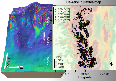
2. Study Area
Climate Setting
3. Dataset and Methodology
3.1. Sentinel-1 DInSAR Applied to Dry Andes
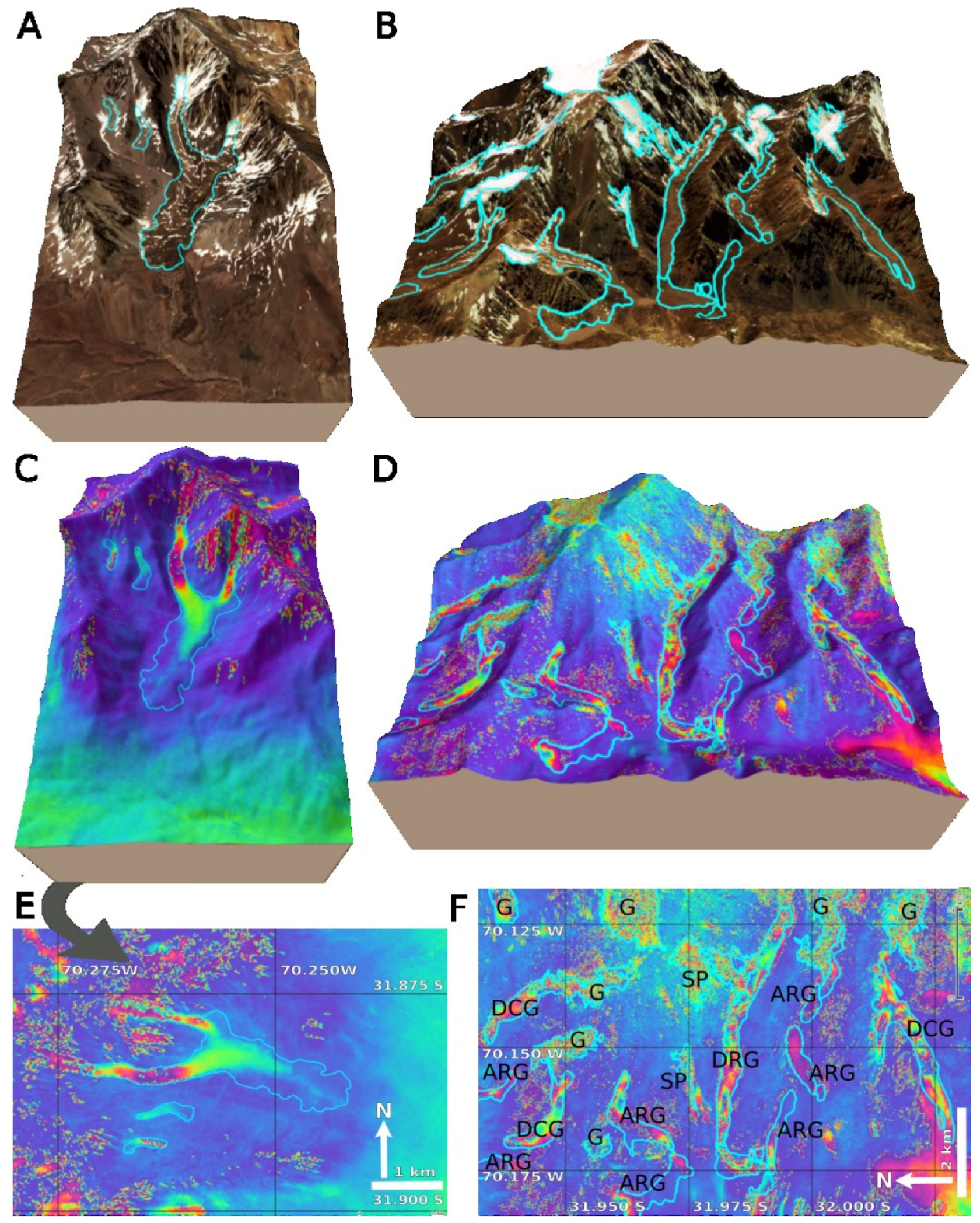
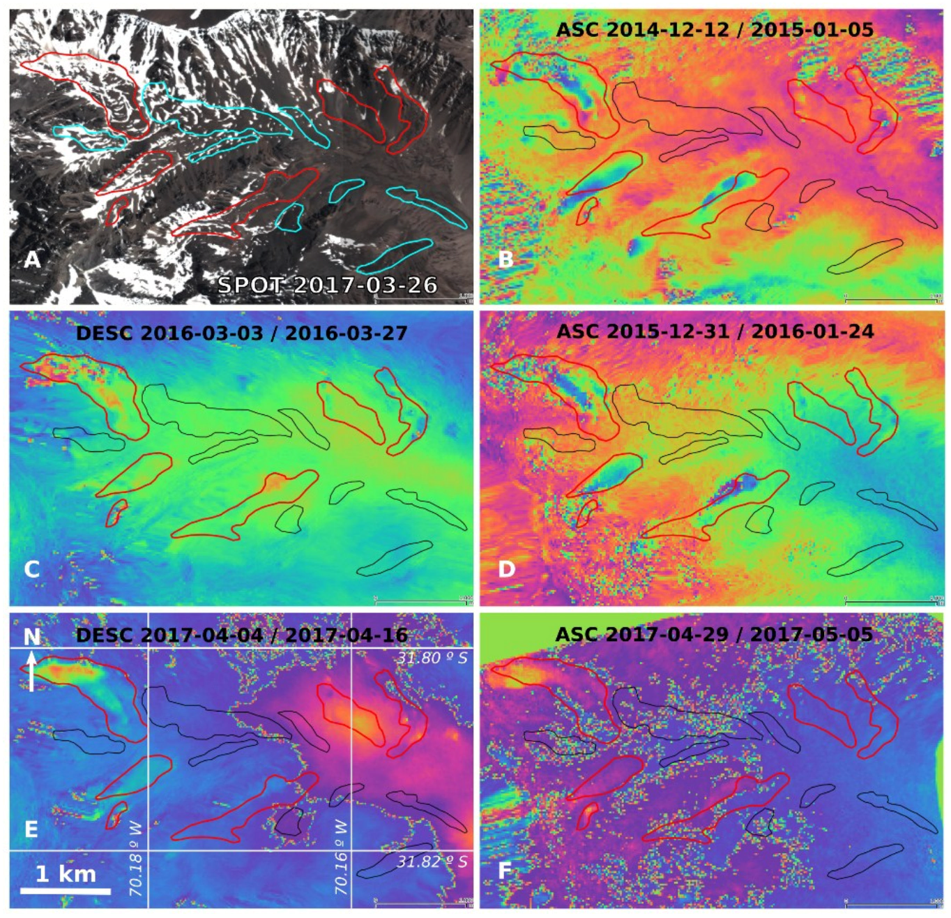
3.2. Active Landforms Detection with DInSAR
3.3. Comparison of DInSAR and Optical Based Inventories
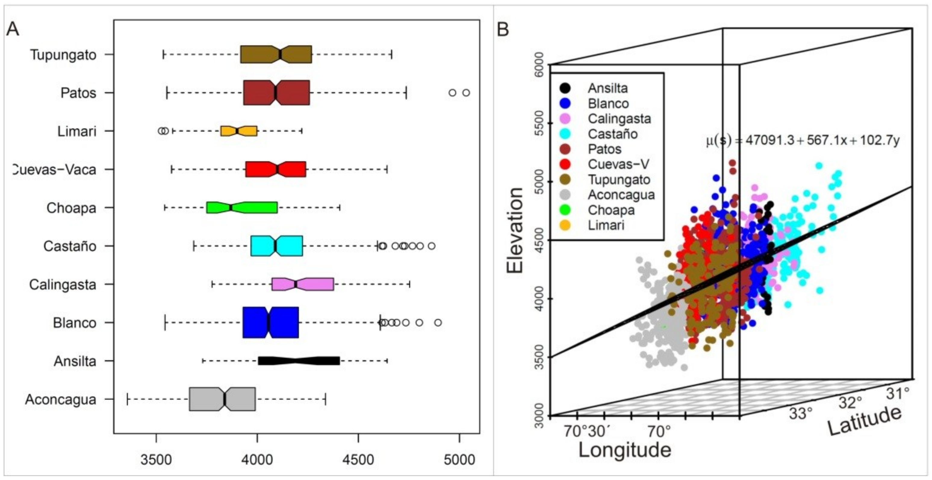
3.4. Statistical Analysis
4. Results
4.1. Comparison between DInSAR and Optical Inventories
4.2. Analysis of the Spatial Structural Model
5. Discussion
6. Conclusions
Author Contributions
Funding
Acknowledgments
Conflicts of Interest
References
- Azócar, G.F.; Brenning, A.; Bodin, X. Permafrost distribution modelling in the semi-arid Chilean Andes. Cryosphere 2017, 11, 877–890. [Google Scholar] [CrossRef]
- Corte, A.E.E.; Corte, L.E.A.E.; Espizua, L.E. Inventario de glaciares de la cuenca del río Mendoza. In Technical Report, Consejo Nacional de Investigaciones Científicas y Técnicas; Instituto Argentino de Nivología y Glaciología: Mendoza, Argentina, 1981. [Google Scholar]
- Brenning, A.; Trombotto, D. Logistic regression modelling of rock glacier and glacier distribution: Topographic and climatic controls in the semi-arid Andes. Geomorphology 2006, 81, 141–154. [Google Scholar] [CrossRef]
- Esper Angillieri, M.Y.E. A preliminary inventory of rock glaciers at 30° S latitude, cordillera frontal of San Juan, Argentina. Quat. Int. 2009, 195, 151–157. [Google Scholar] [CrossRef]
- Wang, X.; Liu, L.; Zhao, L.; Wu, T.; Li, Z.; Liu, G. Mapping and inventorying active rock glaciers in the northern Tien Shan of China using satellite SAR interferometry. Cryosphere 2017, 11, 997–1014. [Google Scholar] [CrossRef]
- Barboux, C.; Strozzi, T.; Delaloye, R.; Wegmuller, U.; Collet, C. Mapping slope movements in alpine environments using Tterrasar-X interferometric methods. ISPRS J. Photogramm. Remote Sens. 2015, 109, 178–192. [Google Scholar] [CrossRef]
- Callegari, M.; Cantone, A.; Cuozzo, G.; Defilippi, M.; Notarnicola, C.; Pasquali, P.; Riccardi, P.; Seppi, R.; Seppi, S.; Zucca, F. Combining Radarsat-2 and Cosmo-Skymed data for alpine permafrost deformation monitoring. In Proceedings of the IEEE International Geoscience and Remote Sensing Symposium (IGARSS), Milan, Italy, 26–31 July 2015; pp. 5260–5263. [Google Scholar]
- Liu, L.; Millar, C.I.; Westfall, R.D.; Zebker, H.A. Surface motion of active rock glaciers in the Sierra Nevada, California, USA: Inventory and a case study using InSAR. Cryosphere 2013, 7, 1109. [Google Scholar] [CrossRef]
- Roer, I.; Nyenhuis, M. Rockglacier activity studies on a regional scale: comparison of geomorphological mapping and photogrammetric monitoring. Earth Surf. Process. Landf. 2007, 32, 1747–1758. [Google Scholar] [CrossRef]
- Azocar, G. Modeling of Permafrost Distribution in the Semi-Arid Chilean Andes. Master’s Thesis, University of Waterloo, Waterloo, ON, USA, 2014. [Google Scholar]
- Barboux, C.; Delaloye, R.; Lambiel, C. Inventorying slope movements in an Alpine environment using DInSAR. Earth Surf. Process. Landf. 2014, 39, 2087–2099. [Google Scholar] [CrossRef] [Green Version]
- Kenyi, L.W.; Kaufmann, V. Estimation of rock glacier surface deformation using SAR interferometry data. IEEE Trans. Geosci. Remote Sens. 2003, 41, 1512–1515. [Google Scholar] [CrossRef]
- Rott, H.; Siegel, A. Analysis of mass movements in alpine terrain by means of SAR interferometry. In Proceedings of the IEEE 1999 International Geoscience and Remote Sensing Symposium, Hamburg, Germany, 28 June–2 July 1999. [Google Scholar]
- Kenyi, L.; Kaufmann, V. Detection and quantification of rock glacier deformation using ERS D-InSAR data. In Proceedings of the ERS-Envisat Symposium, Gothenburg, Sweden, 16–20 October 2000. [Google Scholar]
- Nagler, T.; Mayer, C.; Rott, H. Feasibility of DINSAR for mapping complex motion fields of Alpine ice-and rock-glaciers. In Retrieval of Bio-and Geo-Physical Parameters from SAR Data for Land Applications; European Space Agency: Paris, France, 2002; Volume 475, pp. 377–382. [Google Scholar]
- Rignot, E.; Hallet, B.; Fountain, A. Rock glacier surface motion in Beacon Valley, Antarctica, from synthetic-aperture radar interferometry. Geophys. Res. Lett. 2002, 29, 17. [Google Scholar] [CrossRef]
- Lilleøren, K.S.; Etzelmüller, B.; Gärtner-Roer, I.; Kääb, A.; Westermann, S.; Guðmundsson, Á. The distribution, thermal characteristics and dynamics of permafrost in Tröllaskagi, northern Iceland, as inferred from the distribution of rock glaciers and ice-cored moraines. Permafr. Periglac. Process. 2013, 24, 322–335. [Google Scholar] [CrossRef]
- Necsoiu, M.; Onaca, A.; Wigginton, S.; Urdea, P. Rock glacier dynamics in Southern Carpathian Mountains from high-resolution optical and multi-temporal SAR satellite imagery. Remote Sens. Environ. 2016, 177, 21–36. [Google Scholar] [CrossRef] [Green Version]
- Strozzi, T.; Kääb, A.; Frauenfelder, R. Detecting and quantifying mountain permafrost creep from in situ inventory, space-borne radar interferometry and airborne digital photogrammetry. Int. J. Remote Sens. 2004, 25, 2919–2931. [Google Scholar] [CrossRef]
- Trombotto, D.; Buk, E.; Hernández, J. Rock Glaciers in the Southern Central Andes (Approx. 33–34 s), Cordillera frontal, Mendoza, Argentina; Bamberger Geographische Schriften; University of Bamberg Press: Bamberg, Germany, 1999; Volume 19, pp. 145–173. [Google Scholar]
- Barsch, D. Permafrost creep and rock glaciers. Permafr. Periglac. Process. 1992, 3, 175–188. [Google Scholar] [CrossRef]
- Kääb, A.; Frauenfelder, R.; Roer, I. On the response of rock glacier creep to surface temperature increase. Glob. Planet. Chang. 2007, 56, 172–187. [Google Scholar] [CrossRef]
- Schrott, L. Some geomorphological-hydrological aspects of rock glaciers in the Andes (San Juan, Argentina). Zeitschrift Fur Geomorphologie 1996, Suppl.-Bd. 104, 161–173. [Google Scholar]
- Brenning, A. Geomorphological, hydrological and climatic significance of rock glaciers in the Andes of central Chile (33–35 s). Permafr. Periglac. Process. 2005, 16, 231–240. [Google Scholar] [CrossRef]
- Janke, J.R.; Bellisario, A.C.; Ferrando, F.A. Classification of debris-covered glaciers and rock glaciers in the Andes of central Chile. Geomorphology 2015, 241, 98–121. [Google Scholar] [CrossRef]
- Bodin, X.; Thomas, E.; Liaudat, D.T.; Vivero, S.; Pitte, P. Rock glacier activity and distribution in the semi-arid Andes of Chile and Argentina detected from dInSAR. In Proceedings of the International Conference on Permafrost, Potsdam, Germany, 20–24 June 2016. [Google Scholar]
- Janousek, F.N.M.; Fontana, P.; Capone, A.A.; Sosa, G.J.; Euillades, P.A.; Euillades, L.D. Preliminary analysis of the status of rock glaciers using SAR images. In Proceedings of the 2017 XVII Workshop on Information Processing and Control (RPIC), Mar de Plata, Argentina, 20–22 September 2017; pp. 1–5. [Google Scholar]
- Lliboutry, L. Glaciers of Chile and Argentina; Geological Survey Professional Paper; USGS: Reston, VA, USA, 1998; p. 1103. [Google Scholar]
- Gruber, S.; Haeberli, W. Mountain Permafrost; Springer: Berlin, Germany, 2009; pp. 33–44. [Google Scholar]
- Esper Angillieri, M.Y. Permafrost distribution map of San Juan Dry Andes (Argentina) based on rock glacier sites. J. S. Am. Earth Sci. 2017, 73 (Suppl. C), 42–49. [Google Scholar] [CrossRef]
- INDEC (Instituto Nacional de Estadística y Censo). 2010. Available online: http://www.sig.indec.gov.ar/censo2010/ (accessed on 1 September 2017).
- INE (Instituto Nacional de Estadísticas). 2017. Available online: http://palma.ine.cl/demografia/menu/genera/indice.aspx (accessed on 24 August 2017).
- Milana, J.P. Predicción de caudales de ríos alimentados por deshielo mediante balances de energía: Aplicaci´on en los Andes centrales, Argentina. Revista de la Asociación Argentina de Sedimentología 1998, 5, 53–69. [Google Scholar]
- Hearnea, R.R.; Donoso, G. Water institutional reforms in Chile. Water Policy 2005, 7, 53–69. [Google Scholar] [CrossRef]
- Leiva, J.; Cabrera, G.; Lenzano, L. 20 years of mass balances on the Piloto glacier, las Cuevas river basin, mendoza, Argentina. Glob. Planet. Chang. 2007, 59, 10–16. [Google Scholar] [CrossRef]
- Gascoin, S.; Kinnard, C.; Ponce, R.; Macdonell, S.; Lhermitte, S.; Rabatel, A. Glacier contribution to streamflow in two headwaters of the huasco river, dry Andes of Chile. Cryosphere 2011, 5, 1099–1113. [Google Scholar] [CrossRef] [Green Version]
- Masiokas, M.H.; Villalba, R.; Luckman, B.H.; Le Quesne, C.; Aravena, J.C. Snowpack variations in the central Andes of Argentina and Chile, 1951–2005: Large-scale atmospheric influences and implications for water resources in the region. J. Clim. 2006, 19, 6334–6352. [Google Scholar] [CrossRef]
- Brown Fernández, E.; Saldivia Medina, J.E.; South American Technical Advisory Committee. Informe Nacional Sobre la Gestión del Agua en Chile; Global Water Partnership: Stockholm, Sweden, 2000. [Google Scholar]
- Rosegrant, M.W.; Ringler, C.; McKinney, D.C.; Cai, X.; Keller, A.; Donoso, G. Integrated economic-hydrologic water modeling at the basin scale: The Maipo river basin. Agric. Econ. 2000, 24, 33–46. [Google Scholar]
- Cai, X.; Rosegrant, M.W.; Ringler, C. Physical and economic efficiency of water use in the river basin: Implications for efficient water management. Water Resour. Res. 2003, 39. [Google Scholar] [CrossRef] [Green Version]
- Brenning, A.; Azócar, G.F. Minería y glaciares rocosos: Impactos ambientales, antecedentes pol´ıticos y legales, y perspectivas futuras. Revista de Geograf´ıa Norte Grande 2010, 47, 143–158. [Google Scholar] [CrossRef]
- Stehr, A.; Aguayo, M. Snow cover dynamics in Andean watersheds of Chile (32.0–39.5° S) during the years 2000–2016. Hydrol. Earth Syst. Sci. 2017, 21, 5111–5126. [Google Scholar] [CrossRef] [Green Version]
- Valdés-Pineda, R.; Pizarro, R.; García-Chevesich, P.; Valdés, J.B.; Olivares, C.; Vera, M.; Abarza, A. Water governance in Chile: Availability, management and climate change. J. Hydrol. 2014, 519, 2538–2567. [Google Scholar] [CrossRef]
- Minetti, J.; Vargas, W.; Vega, B.; Costa, M. Las sequias en la pampa húmeda: Impacto en la productividad del maíz. Revista Brasileira de Meteorología 2007, 22, 218–232. [Google Scholar] [CrossRef]
- Montecinos, A.; Díaz, A.; Aceituno, P. Seasonal diagnostic and predictability of rainfall in subtropical South America based on tropical pacific SST. J. Clim. 2000, 13, 746–758. [Google Scholar] [CrossRef]
- Bolius, D.; Schwikowski, M.; Jenk, T.; Gaggeler, H.W.; Casassa, G.; Rivera, A. A first shallow firn-core record from glaciar la ollada, cerro mercedario, central argentine Andes. Ann. Glaciol. 2006, 43, 14–22. [Google Scholar] [CrossRef]
- Corripio, J.; Purves, R.; Rivera, A. Modeling climate change impacts on mountain glaciers and water resources in the central dry Andes. In Darkening Peaks: Glacier Retreat, Science and Society; University of California Press: Berkeley, CA, USA, 2007; pp. 126–135. [Google Scholar]
- Núñez, J.; Rivera, D.; Oyarz´un, R.; Arumí, J. Influence of pacific ocean multidecadal variability on the distributional properties of hydrological variables in north-central Chile. J. Hydrol. 2013, 501, 227–240. [Google Scholar] [CrossRef]
- González-Reyes, Á.; McPhee, J.; Christie, D.A.; Le Quesne, C.; Szejner, P.; Masiokas, M.H.; Villalba, R.; Muñoz, A.A.; Crespo, S. Spatiotemporal variations in hydroclimate across the Mediterranean Andes (30°–37° S) since the early twentieth century. J. Hydrometeorol. 2017, 18, 1929–1942. [Google Scholar] [CrossRef]
- Rutllant, J.; Garreaud, R. Episodes of strong flow down the western slope of the subtropical Andes. Mon. Weather Rev. 2004, 132, 611–622. [Google Scholar] [CrossRef]
- Kalthoff, N.; Bischoff-Gauß, I.; Fiebig-Wittmaack, M.; Fiedler, F.; Thürauf, J.; Novoa, E.; Pizarro, C.; Castillo, R.; Gallardo, L.; Rondanelli, R.; et al. Mesoscale wind regimes in Chile at 30 S. J. Appl. Meteorol. 2002, 41, 953–970. [Google Scholar] [CrossRef]
- Strecker, M.; Alonso, R.; Bookhagen, B.; Carrapa, B.; Hilley, G.; Sobel, E.; Trauth, M. Tectonics and climate of the southern central Andes. Annu. Rev. Earth Planet. Sci. 2007, 35, 747–787. [Google Scholar] [CrossRef]
- Jenk, T.; Graesslin-Ciric, A.; Tobler, L.; Gäggeler, H.; Morgenstern, U.; Casassa, G.; Luthi, M.; Schmitt, J.; Eichler, A.; Schwikowski, M. The Mercedario ice core-an excellent archive for enso reconstruction. In Proceedings of the EGU General Assembly Conference Abstracts, Vienna, Austria, 12–17 April 2015. [Google Scholar]
- Schrott, L. Global solar radiation, soil temperature and permafrost in the central Andes, Argentina: A progress report. Permafr. Periglac. Process. 1991, 2, 59–66. [Google Scholar] [CrossRef]
- Falvey, M.; Garreaud, R.D. Regional cooling in a warming world: Recent temperature trends in the southeast pacific and along the west coast of subtropical South America (1979–2006). J. Geophys. Res. Atmos. 2009. [Google Scholar] [CrossRef]
- Poblete, A.G.; Minetti, J.L. Influye el calentamiento global en la disminución de las nevadas en los Andes Áridos. Revista Universitaria de Geografía 2017, 26, 11–29. [Google Scholar]
- Pellicciotti, F.; Ragettli, S.; Carenzo, M.; McPhee, J. Changes of glaciers in the Andes of Chile and priorities for future work. Sci. Total Environ. 2014, 493, 1197–1210. [Google Scholar] [CrossRef] [PubMed]
- Azócar, G.; Brenning, A. Hydrological and geomorphological significance of rock glaciers in the dry Andes, Chile (27–33 s). Permafr. Periglac. Process. 2010, 21, 42–53. [Google Scholar] [CrossRef]
- Haeberli, W.; Noetzli, J.; Arenson, L.; Delaloye, R.; Gärtner-Roer, I.; Gruber, S.; Phillips, M. Mountain permafrost: Development and challenges of a young research field. J. Glaciol. 2010, 56, 1043–1058. [Google Scholar] [CrossRef] [Green Version]
- Bamler, R.; Hartl, P. Synthetic aperture radar interferometry. Inverse Probl. 1998, 14, R1–R54. [Google Scholar] [CrossRef]
- Barra, A.; Monserrat, O.; Mazzanti, P.; Esposito, C.; Crosetto, M.; Scarascia Mugnozza, G. First insights on the potential of Sentinel-1 for landslides detection. Geomat. Nat. Hazards Risk 2016, 7, 1874–1883. [Google Scholar] [CrossRef]
- Barra, A.; Solari, L.; Béjar-Pizarro, M.; Monserrat, O.; Bianchini, S.; Herrera, G.; Crosetto, M.; Sarro, R.; González-Alonso, E.; Mateos, R.M.; et al. A Methodology to Detect and Update Active Deformation Areas Based on Sentinel-1 SAR Images. Remote Sens. 2017, 9, 1002. [Google Scholar] [CrossRef]
- Huang, Q.; Crosetto, M.; Monserrat, O.; Crippa, B. Displacement monitoring and modelling of a high-speed railway bridge using C-band Sentinel-1 data. ISPRS J. Photogramm. Remote Sens. 2017, 128, 204–211. [Google Scholar] [CrossRef]
- Franceschetti, G.; Lanari, R. Synthetic Aperture Radar Processing; CRC Press: Boca Raton, FL, USA, 1999. [Google Scholar]
- ESA. ESA Copernicus Open Access Hub. 2017. Available online: https://scihub.copernicus.eu/ (accessed on 20 October 2017).
- Crosetto, M.; Monserrat, O.; Cuevas, M.; Crippa, B. Spaceborne differential SAR interferometry: Data analysis tools for deformation measurement. Remote Sens. 2011, 3, 305–318. [Google Scholar] [CrossRef]
- Farr, T.G.; Rosen, P.A.; Caro, E.; Crippen, R.; Duren, R.; Hensley, S.; Seal, D. The shuttle radar topography mission. Rev. Geophys. 2007, 45. [Google Scholar] [CrossRef]
- Barsch, D. Rock Glaciers, Indicators for the Permafrost and Former Geoecology in High Mountain Environment, Series in the Physical Environment; Springer: Berlin, Germany, 1996. [Google Scholar]
- Quantum, G. Development Team, 2012. In Quantum GIS Geographic Information; 2014; (https://qgis.org). [Google Scholar]
- Forte, A.; Villarroel, C.; Esper Angillieri, M. Impact of natural parameters on rock glacier development and conservation in subtropical mountain ranges. Northern sector of the Argentine Central Andes. Cryosphere Discuss. 2016. [Google Scholar] [CrossRef]
- Delaloye, R.; Perruchoud, E.; Avian, M.; Kaufmann, V.; Bodin, X.; Hausmann, H.; Ikeda, A.; Kääb, A.; Kellerer-Pirklbauer, A.; Krainer, K.; et al. Recent interannual variations of rock glacier creep in the European Alps. In Proceedings of the 9th International Conference on Permafrost, Fairbanks, AK, USA, 28 June–3 July 2008; Volume 29, pp. 343–348. [Google Scholar]
- Martin, E.; Whalley, W.B. Rock glaciers: Part 1: Rock glacier morphology: Classification and distribution. Prog. Phys. Geogr. 1987, 11, 260–282. [Google Scholar] [CrossRef]
- Ikeda, A.; Matsuoka, N. Pebbly versus bouldery rock glaciers: Morphology, structure and processes. Geomorphology 2006, 73, 279–296. [Google Scholar] [CrossRef]
- Schmid, M.; Baral, P.; Gruber, S.; Shahi, S.; Shrestha, T.; Stumm, D.; Wester, P. Assessment of permafrost distribution maps in the Hindu Kush Himalayan region using rock glaciers mapped in Google Earth. Cryosphere 2015, 9, 2089–2099. [Google Scholar] [CrossRef]
- Tamburini Beliveau, G. Magnitudes y Características de los Procesos Geodinámicos en el Ambiente Glacial y Periglacial del Cordón de la Ramada (Andes Centrales Argentinos) Mediante Técnicas de Teledetección. Ph.D. Thesis, FCEIA—Universidad Nacional de Rosario, Rosario, Santa Fe, Argentina, 2017. [Google Scholar]
- Johnson, B.G.; Thackray, G.D.; Van Kirk, R. The effect of topography, latitude, and lithology on rock glacier distribution in the Lemhi Range, central Idaho, USA. Geomorphology 2007, 91, 38–50. [Google Scholar] [CrossRef]
- Kenner, R.; Magnusson, J. Estimating the effect of different influencing factors on rock glacier development in two regions in the Swiss Alps. Permafr. Periglac. Process. 2017, 28, 195–208. [Google Scholar] [CrossRef]
- Croce, F.A.; Milana, J.P. Internal structure and behaviour of a rock glacier in the arid Andes of Argentina. Permafr. Periglac. Process. 2002, 13, 289–299. [Google Scholar] [CrossRef]
- Milana, J.P.; Güell, A. Diferencias mecánicas e hídricas del permafrost en glaciares de rocas glacigénicos y criogénicos, obtenidas de datos sísmicos en el tapado, Chile. Revista de la Asociación Geológica Argentina 2008, 63, 310–325. [Google Scholar]
- Bodin, X.; Rojas, F.; Brenning, A. Status and evolution of the cryosphere in the Andes of Santiago (Chile, 33.5°S.). Geomorphology 2010, 118, 453–464. [Google Scholar] [CrossRef]


| Temporal Baseline [Days] | Minimum Detectable Displacement [cm/Year] | Maximum Detectable Displacement [cm/Year] |
|---|---|---|
| 6 | 17 | 170 |
| 12 | 8.5 | 85.2 |
| 24 | 4.2 | 42.6 |
| 36 | 2.9 | 28.4 |
| 48 | 2.2 | 21.3 |
| Master Image Date | Slave Image Date | Temporal Baseline [Days] | Perpendicular Baseline |
|---|---|---|---|
| Ascending 1 | |||
| 4 April 2015 | 28 April 2015 | 24 | 14 |
| 17 Januarty 2016 | 10 February 2016 | 24 | −32 |
| 10 February 2016 | 5 March 2016 | 24 | −52 |
| 5 March 2016 | 29 March 2016 | 24 | 61 |
| 29 April 2017 | 5 May 2017 | 6 | −51 |
| Ascending 2 | |||
| 12 December 2014 | 5 Janury 2015 | 24 | 37 |
| 5 May 2015 | 22 June 2015 | 48 | 65 |
| 31 December 2015 | 24 January 2016 | 24 | 14 |
| 24 January 2016 | 17 February 2016 | 24 | 32 |
| 17 February 2016 | 12 March 2016 | 24 | 26 |
| Descending 1 | |||
| 15 January 2016 | 3 March 2016 | 48 | 46 |
| 3 March 2016 | 27 March 2016 | 24 | −12 |
| Descending 2 | |||
| 8 June 2015 | 2 July 2015 | 24 | −57 |
| 15 February 2016 | 27 February 2016 | 12 | 16 |
| 27 February 2016 | 22 March 2016 | 24 | −43 |
| 4 April 2017 | 16 April 2017 | 12 | −25 |
| Amount of Active Rock Glaciers (ARG) | ||||
|---|---|---|---|---|
| Basin | ARG | DCG-RG | % Difference | |
| DInSAR | Optical | Optical | DInSAR-Optical | |
| Calingasta | 86 | 141 | 11 | −43.4% |
| Ansilta | 36 | 133 | 6 | −74.1% |
| Blanco | 540 | 884 | 20 | −40.2% |
| Los Patos | 339 | 501 | 35 | −36.7% |
| Castaño | 226 | 380 | 6 | −41.4% |
| Cuevas-Vacas | 130 | 189 | 17 | −36.7% |
| Tupungato | 167 | 294 | 38 | −49.7% |
| Total | 1524 | 2522 | 133 | |
© 2018 by the authors. Licensee MDPI, Basel, Switzerland. This article is an open access article distributed under the terms and conditions of the Creative Commons Attribution (CC BY) license (http://creativecommons.org/licenses/by/4.0/).
Share and Cite
Villarroel, C.D.; Tamburini Beliveau, G.; Forte, A.P.; Monserrat, O.; Morvillo, M. DInSAR for a Regional Inventory of Active Rock Glaciers in the Dry Andes Mountains of Argentina and Chile with Sentinel-1 Data. Remote Sens. 2018, 10, 1588. https://doi.org/10.3390/rs10101588
Villarroel CD, Tamburini Beliveau G, Forte AP, Monserrat O, Morvillo M. DInSAR for a Regional Inventory of Active Rock Glaciers in the Dry Andes Mountains of Argentina and Chile with Sentinel-1 Data. Remote Sensing. 2018; 10(10):1588. https://doi.org/10.3390/rs10101588
Chicago/Turabian StyleVillarroel, Cristian Daniel, Guillermo Tamburini Beliveau, Ana Paula Forte, Oriol Monserrat, and Monica Morvillo. 2018. "DInSAR for a Regional Inventory of Active Rock Glaciers in the Dry Andes Mountains of Argentina and Chile with Sentinel-1 Data" Remote Sensing 10, no. 10: 1588. https://doi.org/10.3390/rs10101588