Article

Advancing Precipitation Estimation and Streamflow Simulations in Complex Terrain with X-Band Dual-Polarization Radar Observations

by
Marios N. Anagnostou
1,2,3,*,
Efthymios I. Nikolopoulos
4,
John Kalogiros
1,
Emmanouil N. Anagnostou
4,
Francesco Marra
5,
Elisabeth Mair
6,
Giacomo Bertoldi
6,
Ulrike Tappeiner
6,7 and
Marco Borga
8
1
National Observatory of Athens, IERSD, 15236 Athens, Greece
2
Department of Environmental Engineering, School of Engineering, DUTH, 67100 Xanthi, Greece
3
Department of Water Resources, School of Civil Engineering, NTUA, 10682 Athens, Greece
4
Civil and Environmental Engineering, School of Engineering, University of Connecticut, Hartford, CT 06269, USA
5
Institute of Earth Sciences, Hebrew University of Jerusalem, Jerusalem 9190401, Israel
6
Institute for Alpine Environment, Eurac research, 39100 Bolzano, Italy
7
Department of Ecology, University of Innsbruck, Innsbruck A-6020, Austria
8
Department of Land, Environment, Agriculture and Forestry, University of Padova, 35122 Padova, Italy
*
Author to whom correspondence should be addressed.
Remote Sens. 2018, 10(8), 1258; https://doi.org/10.3390/rs10081258
Submission received: 26 June 2018 / Revised: 22 July 2018 / Accepted: 6 August 2018 / Published: 10 August 2018
(This article belongs to the Special Issue Remote Sensing of Precipitation)

Abstract

:
In mountain basins, the use of long-range operational weather radars is often associated with poor quantitative precipitation estimation due to a number of challenges posed by the complexity of terrain. As a result, the applicability of radar-based precipitation estimates for hydrological studies is often limited over areas that are in close proximity to the radar. This study evaluates the advantages of using X-band polarimetric (XPOL) radar as a means to fill the coverage gaps and improve complex terrain precipitation estimation and associated hydrological applications based on a field experiment conducted in an area of Northeast Italian Alps characterized by large elevation differences. The corresponding rainfall estimates from two operational C-band weather radar observations are compared to the XPOL rainfall estimates for a near-range (10–35 km) mountainous basin (64 km2). In situ rainfall observations from a dense rain gauge network and two disdrometers (a 2D-video and a Parsivel) are used for ground validation of the radar-rainfall estimates. Ten storm events over a period of two years are used to explore the differences between the locally deployed XPOL vs. longer-range operational radar-rainfall error statistics. Hourly aggregate rainfall estimates by XPOL, corrected for rain-path attenuation and vertical reflectivity profile, exhibited correlations between 0.70 and 0.99 against reference rainfall data and 21% mean relative error for rainfall rates above 0.2 mm h−1. The corresponding metrics from the operational radar-network rainfall products gave a strong underestimation (50–70%) and lower correlations (0.48–0.81). For the two highest flow-peak events, a hydrological model (Kinematic Local Excess Model) was forced with the different radar-rainfall estimations and in situ rain gauge precipitation data at hourly resolution, exhibiting close agreement between the XPOL and gauge-based driven runoff simulations, while the simulations obtained by the operational radar rainfall products resulted in a greatly underestimated runoff response.

1. Introduction

Natural disasters occurring in mountainous areas worldwide are most often associated with hazards like flash floods, debris flows, and landslides, which are responsible for fatalities, property losses, and environmental degradation [1,2]. The triggering process of those hazards depends on several factors including hydrological, geomorphological, and geotechnical features [3], but indisputably, the primary triggering factor is heavy rainfall interacting with a steep topography. Given the prospect of increase in frequency and intensity of heavy precipitation events in the context of climate change [4,5], the risk associated with rainfall-induced hazards is expected to increase in the future.
Early warning systems are essential elements in the development of disaster preparedness and response strategies [6,7]. The effectiveness of early warning procedures depends highly on the accuracies of the precipitation monitoring systems involved [4,8,9]. The impact of accurate representation of rainfall spatial variability on simulating the flash flood response has been demonstrated by several studies [10,11,12]. Moreover, recent studies [13,14] have shown the importance of accurate rainfall estimates at small spatial scales for the prediction of debris flow/landslide initiation. Therefore, to improve the accuracy of flood hazard warning systems, it is critical to acquire accurate estimates of precipitation rates at a high resolution.
The quantification of precipitation over mountainous areas, where these phenomena typically occur, is rather complex, and topography plays a dominant role in shaping precipitation variability [15]. Current operational rainfall monitoring systems from national weather radar networks do not provide sufficiently accurate measurements of precipitation variability over mountainous areas [16]. Oftentimes, storms developing in mountainous regions are affected by low-level orographic enhancement of precipitation that affects both the small-scale variability and intensity of rain rates and creates a great challenge to Quantitative Precipitation Estimation (QPE) by weather radar observations [17,18]. For operational radar networks, in particular, the monitoring of precipitation at long ranges is associated with precipitation detection issues including partial, or total, beam blockage of the lower beam elevations or overshooting of low-level convection signatures by the upper elevation sweeps, which leads to significant range dependent errors in the quantification of surface rainfall [19,20]. In addition, melting snow in widespread storm systems that typically result in high accumulations from persistent stratiform precipitation may substantially increase the threat of localized flash floods in mountainous basins [21].
Past studies [22,23,24,25,26,27,28,29] have shown that locally deployed dual-polarization X-band radar systems can contribute higher resolution rain rate estimations and improved rainfall quantification accuracies than the lower frequency (C-band and S-band) long-range operational radar systems. These short-range radar systems could potentially be used to fill in coverage gaps of operational weather radar networks, which is particularly important for advancing early warning of precipitation driven hydrological hazards (flash floods, landslides, debris flows, etc.) in urban and small mountainous basins [24,25,30]. A key drawback of X-band radar wavelength in rainfall estimation is the severe rain-path attenuation, but dual-polarization radar technology can now mitigate this effect through the development of robust attenuation correction schemes [31,32,33,34,35,36,37,38,39,40,41]. As a result, progress in the X-band dual-polarization rainfall estimation has enhanced the applicability of such radar (typically mobile) systems for flood modeling applications in urban areas [42,43,44,45] and in complex terrain basins [22,23,24,25,31,46,47].
The study’s objective is to evaluate the QPE obtained from locally deployed X-band dual-polarization (XPOL) observations and associated accuracies in hydrologic simulations of small-scale mountainous basins compared to precipitation estimates derived from near-range operational radar (C-band) observations [48]. This study is based on a field experiment conducted in the framework of HyMeX (Hydrological cycle in a Mediterranean experiment) Special Observation Period One (SOP 1) in the summer-fall period of 2012 and 2014 over a mountainous region (above 2000 m elevation ranges) in the Eastern Italian Alps. Quantitative comparisons of precipitation estimate and associated hydrologic simulations between the locally deployed XPOL from this field experiment and near-range operational C-band radars are used to highlight the benefits of locally deployed short-range X-band dual-polarization radar observations in terms of small-scale rainfall and runoff estimations. A description of the study area, the data collected and the setup of the field experiment are provided in the next section. The XPOL rainfall estimation algorithm and evaluation results are discussed in Section 2. Comparison of error statistics between XPOL and the operational C-band rainfall products and corresponding errors in hydrologic simulations are provided in Section 3.1, Section 3.2 and Section 3.3, respectively. Finally, the main conclusions are summarized in Section 4.

2. Instruments and Methodology

In the framework of HyMeX Special Observation experiment, the National Observatory of Athens (NOA) XPOL mobile radar was deployed in the northwestern part of Upper Adige river basin, in Eastern Italian Alps in July through October periods of 2012 and 2014 (Figure 1).
XPOL was deployed at an elevation of 2060 m (46°34′10.56″, 10°30′41.7594″) near range (40 km) of an experimental mountainous basin exhibiting dense in situ observations [49,50,51], which is part of the Long Term (Socio) Ecological Research site Matsch/Mazia (http://lter.eurac.edu/en). The upper Saldur catchment is located, with reference to its outlet, 10 km northeast from the XPOL site (Figure 1) and comprises the study area for the hydrologic analysis presented in this work. The basin covers a highly complex terrain area of 62 km2 with elevations ranging from about 1400 to 3700 m a.s.l. and an average elevation of about 2500 m a.s.l. At the upper part of the basin, a significant portion of the area (2.8 km2 in 2013) [52] is covered by glaciers. Due to its inner-alpine position, the mean annual precipitation in the lower valley is lower than 530 mm at 1600 m a.s.l. (Source: Mazia meteorological and discharge measurement stations of the Hydrographic Office South Tyrol). However, a strong lapse rate leads to more than 1000 mm year−1 at the higher altitudes of the basin, which touch the Alps main divide [53]. Precipitation typically occurs as snowfall from November to late April, but snowstorms can also occur during the summer and early fall at the higher elevations. During the late summer-early fall (the period of this experiment) precipitation typically originates from convective rainfall [54].
During the experimental periods, rainfall data were collected from the XPOL and a dense network of in situ sensors (rain gauges, meteorological stations, and disdrometers) contributed by the NOA, Eurac research (Bozen/Bolzano), and the hydrologic office of the Autonomous Province of Bolzano. Available instrumentation used in this study, shown in Figure 1, includes one 2D-video disdrometer (2DVD) available only in 2012 period, one laser type Parsivel disdrometer (APU), fourteen rain gauges, and seven meteorological stations with the temporal resolution of 15 min [55]. Three of the rain gauge stations also provided snow depth data. Since most of the rain gauges are in high altitudes and none of them are heated, liquid precipitation is distinguished from snow using air temperature and snow-depth observations in order to avoid rainfall underestimations [56].
The XPOL radar was operated during rain events first in plan position indicator (PPI) mode taking measurements in a sector scan of 60°, at 0.5°, 1.5°, 2.5°, 3.5°, and 5° elevation sweeps with a range resolution of 120 m for a total range of 35 km. The radar also operated in a range height indicator (RHI) mode taking RHI measurements over the two disdrometer sites. The antenna rotation rate was 6 deg s−1 for PPI and 3 deg s−1 for RHI mode. The time period for a full volume scan including the RHIs was less than 3 min.
The study domain is also covered by two operational C-band radar networks, one from Austria (~60 km from study basin) and a second from Switzerland (~150 km from study basin), providing surface QPE maps. The Austrian Meteo Service network covers the study area with a C-band weather radar located at the Valluga Mountain (2809 m a.s.l.); hereafter named “Valluga”. The radar covers the western parts of the Austrian Alps in the borders with the Italian Alps (shown in Figure 1). The lowest usable elevation is −0.5°, and a volume scan consists of 16 elevation sweeps with a duration of 5 min [57]. Technical details of the Valluga C-band radar are listed in Table 1. The rainfall maps from this radar are based on an algorithm described in [58,59]. Surface QPE maps are available at 1 km grid resolution and hourly accumulations.
The second operational radar rainfall product over the study area is based on estimates from the MeteoSwiss weather radar network covering the area [60]; specifically, the MeteoSwiss radar observations over the study area are based on three dual-polarization C-band radars located at Mt Lema, La Dôle, and Albis in Switzerland (technical characteristics described in Table 1). The rainfall product from the MeteoSwiss operational radar network (hereafter named “Swiss”) is based on an operational rainfall estimation algorithm called “CombiPrecip” [61,62,63] that provides hourly accumulated gauge-adjusted/radar merging rainfall maps at a 1 km grid resolution.
Table 2 summarizes the precipitation events selected in this study during the two experimental periods and the corresponding availability of sensor observations. The table also reports the average rainfall accumulation (in mm) reported from rain gauges deployed in the Saldur catchment. Ten out of the fifteen recorded events over the two experimental periods constitute the dataset of this study. The criteria for selecting these events are the availability of coincident operational C-band radar and XPOL rainfall datasets, in situ observations, and event total rainfall accumulations exceeding 10 mm. The “Swiss” radar rainfall product was used in 2014 and the 25 August 2012 event, while, for the rest of the selected storm events, we used rainfall products from the Valluga radar (Austrian radar network).
Although no major flooding occurred during the two field experiments in the study area, due to the moderate precipitation intensity of the storm events, the streamflow observations (made available from the Hydrologic Office of the Autonomous Province of Bolzano) show that two of the recorded events were associated with basin response adequate to support flood modeling. Therefore, in addition to the precipitation data, discharge observations for three different locations at the Saldur basin are used in this study to verify the model applied for hydrologic simulations.

XPOL Radar Rainfall Estimation Algorithm

This section describes the microphysical algorithm (named SCOP-ME) of Reference [64] applied on the XPOL radar observations. XPOL reflectivity observations were corrected for partial beam blockage and measurement biases prior to applying the precipitation retrieval algorithm. For beam blockage estimation, high-resolution terrain information and a three-dimensional model of the radar beam was applied. This information is used to exclude from further processing highly occluded areas or to correct reflectivity from areas with a minor (<50%) occlusion.
Next, the calibration of the XPOL radar echo signal (horizontal and differential reflectivity) was determined for the correct application of the XPOL radar algorithms. This calibration is assessed by comparing XPOL measurements to reference radar parameters (reflectivity and differential reflectivity) determined using scattering (T-matrix) routines applied on the drop size distribution (DSD) measurements from the 2DVD and Parsivel disdrometers deployed in the study area (both at ~17 km range and directly visible from XPOL). The lowest antenna elevation (0.5°) was used because XPOL observations at this elevation are closest in altitude to the disdrometers, while there is no significant beam blockage or ground clutter affecting the XPOL measurements. The mean bias determined from this process was subsequently removed from the radar data, as is described in more detail in the Kalogiros et al. [64], and it was found to be 3.5 dB and −0.2 dB for the horizontal and differential reflectivity, respectively. These values are close to the calibration biases reported from previous XPOL deployments [22,37].
Figure 2a,b shows scatter plots of the rain-path attenuation corrected and bias-adjusted of XPOL horizontal (ZhR) and differential (ZdrR) reflectivity versus the corresponding ZhD and ZdrD parameters determined by rain spectra observations from the two disdrometers (2DVD—black dot and Parsivel—gray dot) in 2012 (Figure 2a) and only the Parsivel in 2014 (Figure 2b). The bias calibration of ZhR and ZdrR are made using long-term disdrometer data as described in Kalogiros et al. [64] and Anagnostou et al. [37]. The calibration of ZdrR is also improved using a real-time method which is based on average Zh-Zdr relations. It is actually preformed in every radar scan using a Zdr vs. Zh average relation which is dynamically corrected for each scan, as described in more details in Reference [64]. The correlation coefficient of XPOL radar parameters compared to both disdrometers (2DVD and Parsivel) and for both observation years are 0.80 and 0.65 for the horizontal and differential reflectivity, respectively, and the mean relative error (after removing the corresponding biases) is less than 3% for both reflectivity types. Even though the scatter plots (especially the Zdr plot) look noisy due factors like measurements errors, the difference in height between the radar volume and the disdrometer, and the difference in spatial resolution of the two systems (radar volume versus point measurement), what is important is that the mean bias can be reliably estimated despite the scattering. Similar scatter has been observed in past studies over complex terrain [22,23], In addition, as it was mentioned above, the Zdr calibration is actually made in every radar scan using a Zdr vs. Zh average relation [64]. Next, we briefly describe the rainfall retrieval algorithm applied to bias-adjusted XPOL parameters.
The first step of the algorithm is the identification of the rain precipitation regime in each radar ray and application of the SCOP algorithm [36,64]. The path attenuation of a radar signal is significant, especially for high-frequency radars (like X-band). For the correction of path attenuation in rain, the SCOP algorithm is used. This algorithm is a self-consistent polarimetric algorithm, based on the parameterizations of the specific attenuation coefficients and backscattering phase shift in the rain, derived by Kalogiros et al. [64], and applied with an iterative scheme to separate radar rays [64]. Comparison with in situ disdrometer and rain gauge data in past studies [35,36,64] has shown that the attenuation correction procedure described in Reference [64] is more efficient than previous polarimetric attenuation correction algorithms [65,66].
Due to the high elevation of the XPOL deployment in this study, the radar beam frequently intercepted the snow-rain melting layer and the snow region of stratiform precipitation above the study area (40 km range). Thus, to properly estimate rainfall rate at ground level, a correction for the effect of the melting layer and the snow layer above it on the radar measurements was applied. The methodology followed here is an extension of Reference [67] technique applied to PPI scans using the apparent vertical profile of reflectivity (VPR) shape (hereafter called the apparent VPR correction) with temporally variable characteristics determined from the radar data itself [35]. The apparent VPR correction algorithm was used to identify the bright band zone and snow region above, and remove these effects, bringing the spatial variability of reflectivity closer to the actual values below the melting layer (i.e., in the rain layer near the ground provided that the melting layer has not reached the ground level).
After rain-path attenuation and VPR correction, we applied the rainfall estimation and microphysical algorithms defined by Equations (2)–(4d) in Reference [35]. To understand the effectiveness of the VPR correction in rainfall estimation, Figure 3 and Figure 4 show the XPOL rainfall timeseries (before and after the VPR correction for the 1.5° and 3.5° elevation) compared to the corresponding timeseries of rainfall derived from the two disdrometers (i.e., Parsivel and 2DVD) for the rain event of 24 September 2012 and from the Parsivel disdrometer for the rain events of 9 and 12–13 August 2014. When the VPR correction reduces (increases) the rainfall values estimated by XPOL, the radar beam gate at the horizontal position of the in-situ sensor was located in the bright band (above the bright band and in the snow region). Despite the random differences shown in Figure 3b and Figure 4b between the XPOL and in situ rainfall for the high elevation angle (3.5°), the comparison of accumulated rainfall depicted in Figure 3c and Figure 4c, shows that the VPR correction significantly reduces the difference between radar and in situ ground observations. Removing this systematic error in accumulated rainfall is a critical factor in hydrological runoff modeling [68], which will be discussed later in the paper.
Figure 5 and Figure 6 show the PPI of XPOL radar accumulated rainfall estimates without (upper two plots) and with VPR (lower two plots) correction from two high-elevation sweeps (2.5° and 3.5°). It is noted that the spatial structure of accumulated rainfall is similar between the two elevations after removing the bright band overestimation and snow underestimation based on the VPR correction procedure. In Figure 6, it can be seen that the bright band (melting layer) is at a longer range (and, thus, at higher height) than in Figure 5. In Figure 6 its base is at about 2800 m (radar height is about 2100 m), while in Figure 5 its base is at about 2400 m. More precisely, at the range where the base of the bright band is located in 2.5° elevation of Figure 6 the radar beam is completely blocked by the slope of the mountain (i.e., it is too low and interacts with the ground) in the center of the scanning sector and, thus, bright band detection and correction is very difficult for this elevation. The differences in rainfall field between the 2.5° and 3.5° elevations are found before the bright band range (i.e., below its height) and have nothing to do with the VPR correction because no VPR correction is applied below the bright band. These differences are probably due to some ground clutter in the 2.5° elevation PPI, which remained even after the application of the clutter filter. This is the reason that radar data from the 3.5° elevation was used, but not a higher elevation in order to limit the height of the radar volume above the surface and the effect of melting layer at close ranges, for further analysis (Section 3).
Furthermore, scatterplots (Figure 7) of radar rainfall estimates before and after the VPR correction against disdrometer measurements for all the recorded rain events (even the rain events excluded from this study) for both field experiments indicate similar performance with a mean relative error change from about 50% overestimation before VPR correction to less than 10% after the application of the algorithm.
As a final step, XPOL radar rainfall estimates were converted to a Cartesian grid and aggregated to half-hourly rainfall accumulations (in mm h−1). Linear interpolation was used to interpolate from the original polar grid to the Cartesian grid with a 200 × 200 m resolution. The gate resolution of XPOL was 120 m (as it is mentioned in the third paragraph of Section 2) and the angular resolution was 0.6°. Thus, the original polar grid resolution matches, on average, the Cartesian grid resolution in the area of the basins of interest. The XPOL rainfall estimation maps used in this work were processed at a high (200 × 200 m) and coarser (1 × 1 km) grid resolution, comparable with the “Austrian” and “Swiss” radar precipitation products. The 1 × 1 km Cartesian grid was made by averaging the 200 × 200 m grid cells contained in each cell of the coarser grid.

3. Results and Discussion

This section contrasts the quantitative evaluation of high-resolution XPOL rainfall estimates to the operational Swiss and Austrian radar network estimates using error statistics and scatter plots based on in situ rain gauge rainfall observations as a reference. In addition, this section shows a qualitative comparison between XPOL and the two operational radar rainfall products using storm total accumulation maps of two rainfall events (25 August 2012 and 12–13 August 2014) that triggered moderate peak runoff at the Saldur basin outlet.

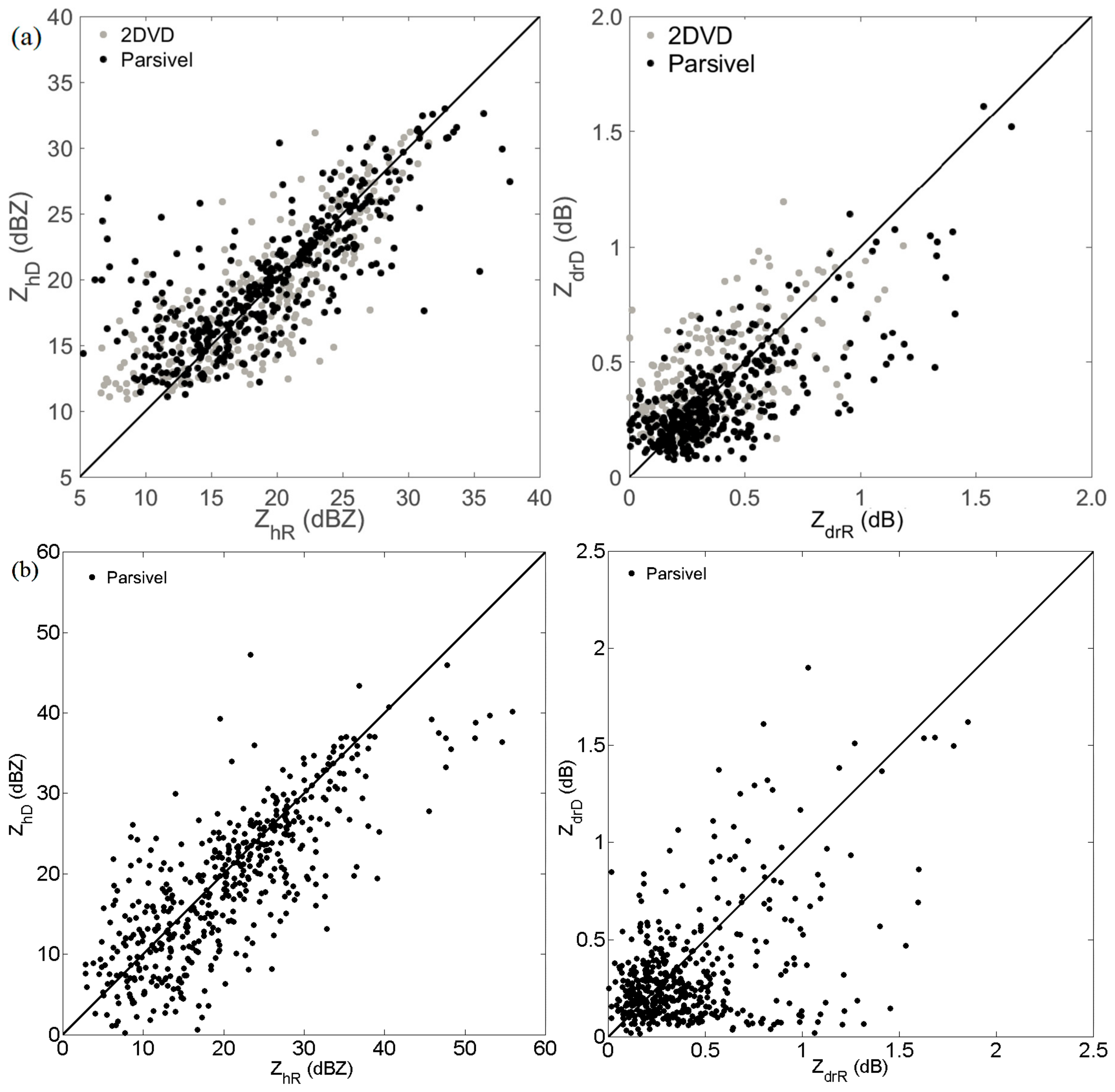
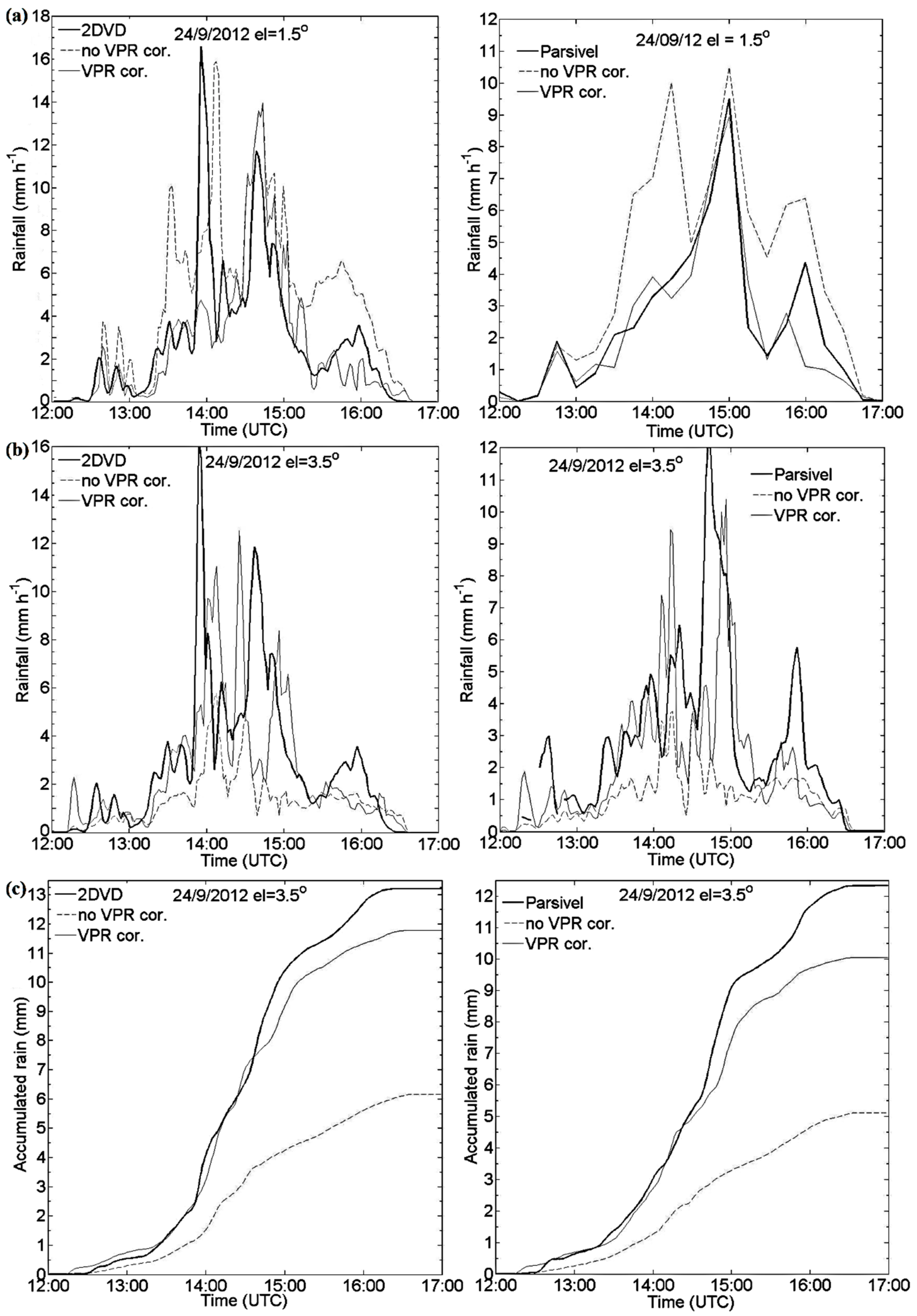
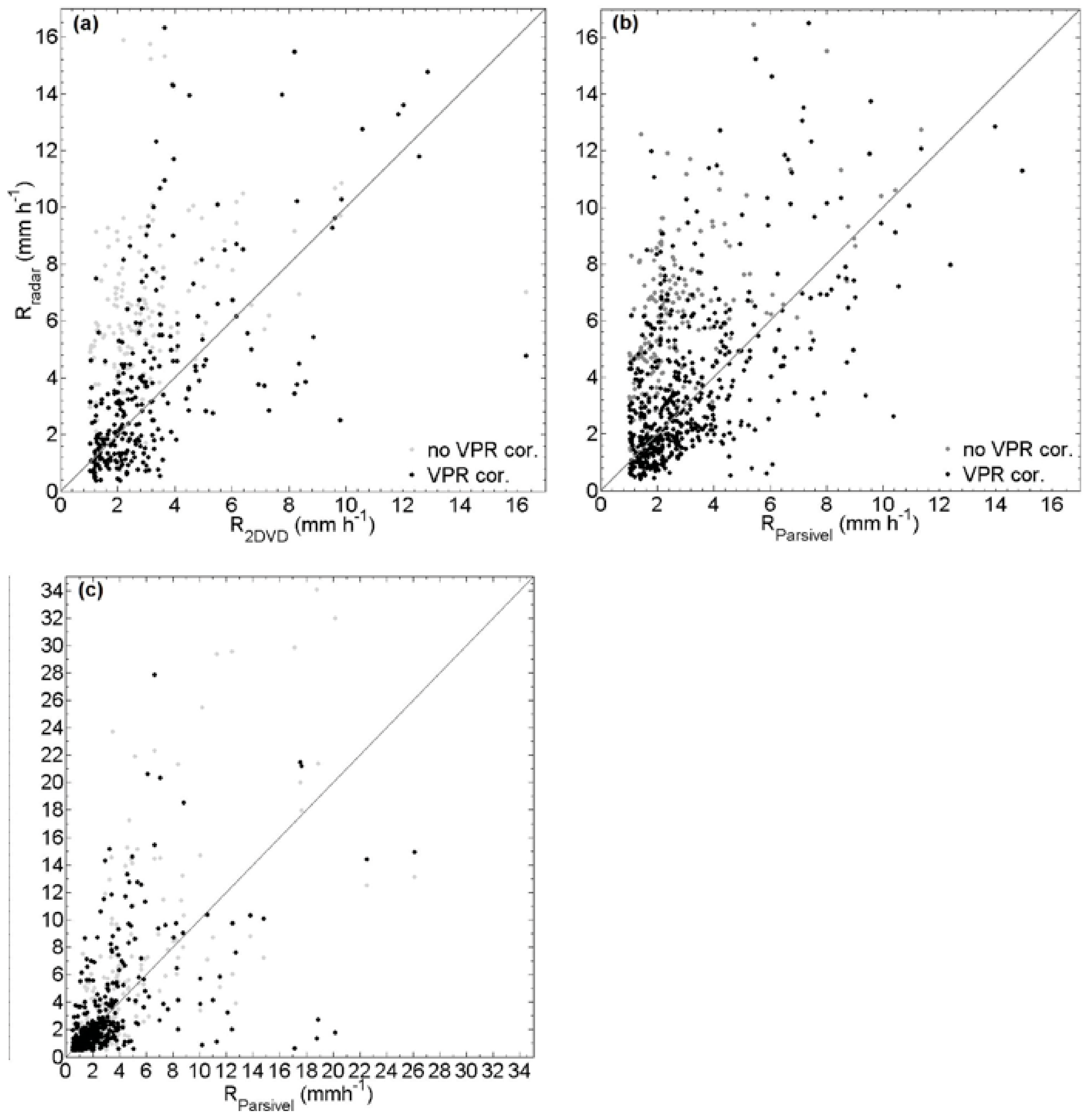
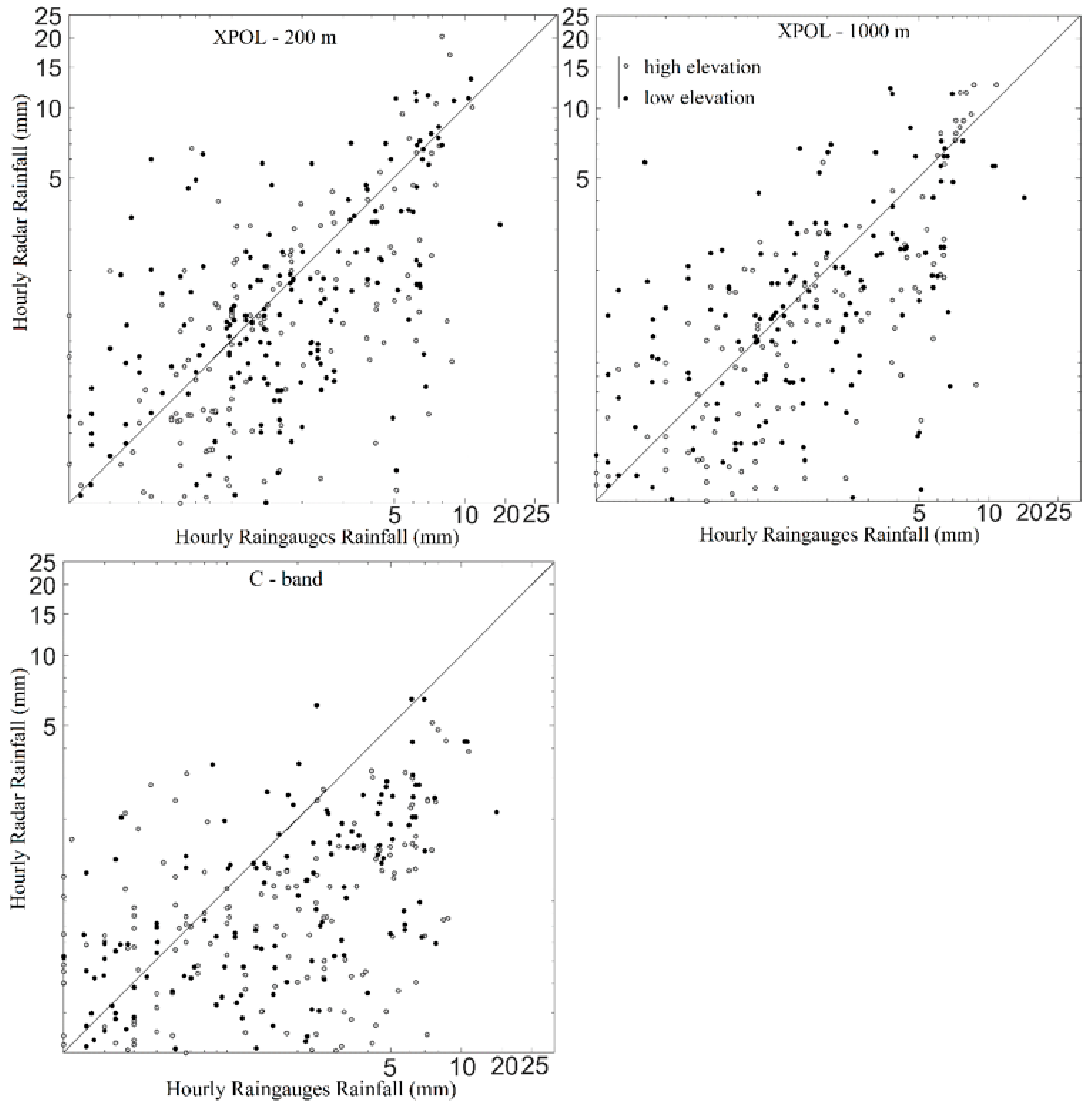
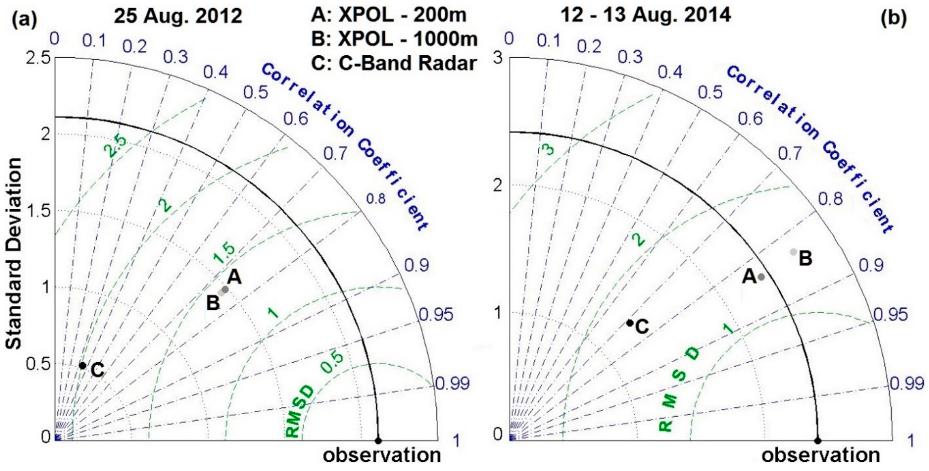
3.1. Quantitative Evaluation of Radar-Rainfall Estimates

The statistical metrics for the evaluation of the radar-rainfall estimates include (1) the correlation coefficient between hourly radar-rainfall estimates and reference rainfall; (2) the unconditional bias ratio, which is defined as the ratio of storm event total radar rainfall estimates to the corresponding reference values; and (3) the conditional bias ratio, which is the same as in (2), but for values of the reference rainfall greater than 0.1 mm h−1. The presented statistical analysis is evaluated based on hourly rainfall accumulation values (in mm h−1) from a network of rain gauges divided into two groups, namely, gauges located inside the Saldur basin with a mean elevation at 2664 m (ranged from 1827 to 3500 m), hereafter named “high-elevation” gauges; and outside the Saldur basin with a mean elevation of 1095 m (ranged from 700 to 1490 m), hereafter named “low-elevation” gauges. The XPOL rainfall estimates are evaluated at both XPOL grid resolutions (200 m and 1 km) to show potential spatial aggregation effects on the error statistics, given that operational radar rainfall estimates are available at a 1-km grid resolution.
A summary of bulk statistical metrics (correlation coefficient, total unconditional and conditional—for reference rainfall > 0.1 mm h−1—biases) of rainfall between estimates (i.e., the two C-band and XPOL radars) and reference (rain gauges) are presented in Table 3. We compared the performance metrics for both high and low elevation gauges. Analyzing the unconditional and conditional biases will provide a metric of rainfall detection error. According to these results XPOL rainfall estimates outperform the operational (C-band based) radar-rainfall products consistently for all events and gauge-elevation groups. Specifically, XPOL rainfall estimates exhibit correlations in the range of 0.70 to 0.99 for the low elevation and 0.62 to 0.99 for the high elevation gauge groups. Both Table 3 and Figure 8 results are for 1 h accumulated rainfall interpolated in an orthogonal grid of 200 m or 1 km resolution, respectively. Thus, a significant amount of spatial and temporal smoothing has been done, which means less random error and higher correlation with rain gauge data. It is important to note here that the 0.99 correlation from the 24/09 event is not statistically significant since the time duration was 5 h (see Figure 3) and, thus, only 5 points from this event were included in Table 3 and Figure 8, results.
On the other hand, the operational radar products show a significantly increased variation in performance with correlation values, being between 0.51 and 0.88 for the low elevation gauge group and 0.48 to 0.71 for the high elevation gauge group. The results for the conditional and unconditional bias ratios show that for the majority of cases, the majority of the operational radar rainfall products exhibit severe underestimation with the bias ratio (both conditional and unconditional) exhibiting values ranging from 0.21 up to 0.91 for the low elevation gauge groups, and from 0.24 up to 0.97 for the high elevation gauge groups. However, there are some cases (i.e., 4 August 2014 and 15 September 2014 events) where the C-band radar rainfall overestimated the surface rainfall.
On the other hand, the XPOL estimates are associated with considerably reduced bias, compared to the C-band estimates, that, although it varies largely among the cases, is on average 30%. A distinct feature from the results reported in Table 3 is an apparent large overestimation of the XPOL rainfall estimates in the last two events of 2014 field experiment (29 August and 15 September) where it reached up to 3-times the rainfall from the reference. In these two events, although the XPOL rainfall estimates did not capture the peak rainfall rate values accurately they performed better for the lower rainfall rates. This can be explained due to the close ground melting layer and missed correction of the VPR algorithm to the rainfall estimate and to the “undercatch” problem of the ground reference (rain gauges) measure during low rainfall rates (<1 mm h−1).
Figure 8 shows scatter plots of hourly rainfall (mm) estimates from the XPOL and the C-band radar products against the low and high elevation gauge-group hourly rainfall accumulations. It is noted that the XPOL rainfall estimates are almost unbiased in moderate to high rainfall values (i.e., >2 mm h−1) for all cases. At the low-elevation gauge group, XPOL rainfall estimates exhibit a systematic overestimation, consistent with the bias statistics discussed above. Bias statistics presented in Table 3 and the scatter plots of Figure 8 suggest that a significant grid resolution effect on the error statistics is present. On the other hand, both Figure 8 and Table 3 results reveal that the longer-range operational C-band radar rainfall estimations systematically underestimated rainfall at both low and high elevation gauge groups. A point to note is that both of these C-band radar rainfall products include operational gauge-based adjustments, though located far away from our study area, while the XPOL rainfall polarimetric estimates are based on the disdrometer-driven radar parameter adjustments and a polarimetric technique that is independent of in situ rainfall measurements [64]. Nevertheless, these are the best operational radar rainfall products available for the study area (the Italian radar network is blind due to beam blockage) and represent in this study the baseline radar-rainfall performance characteristics.

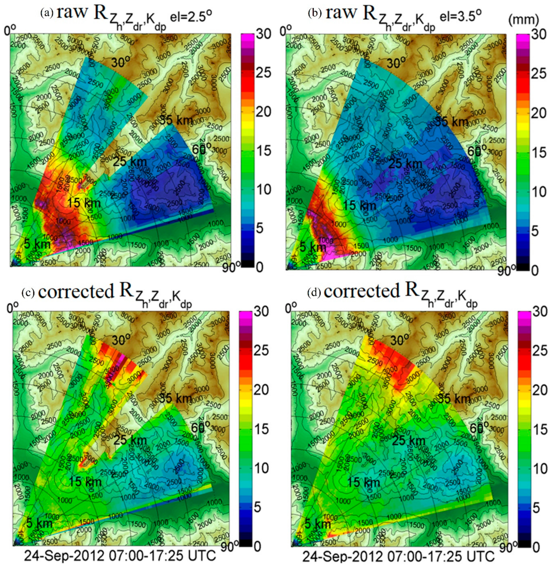
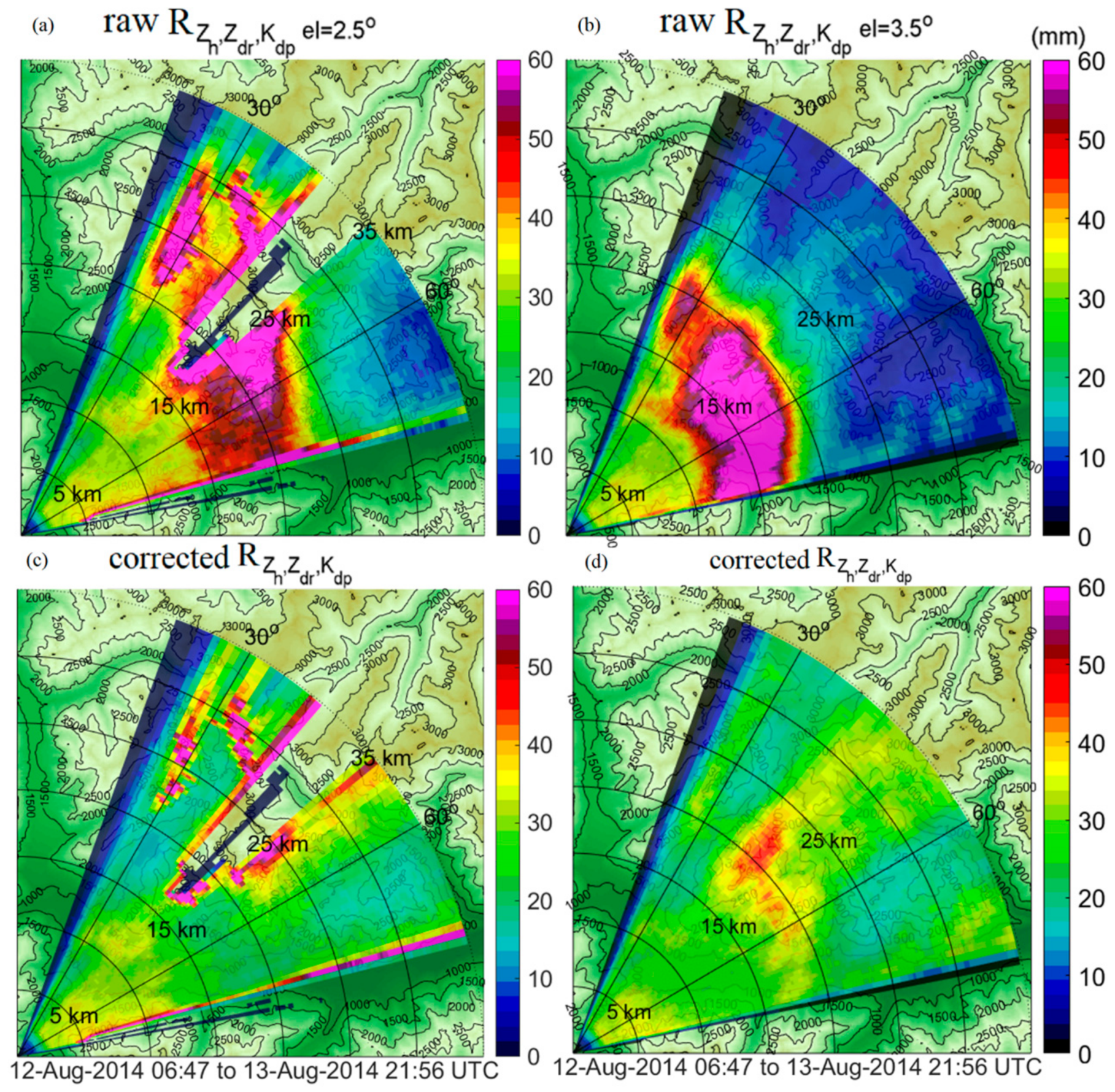
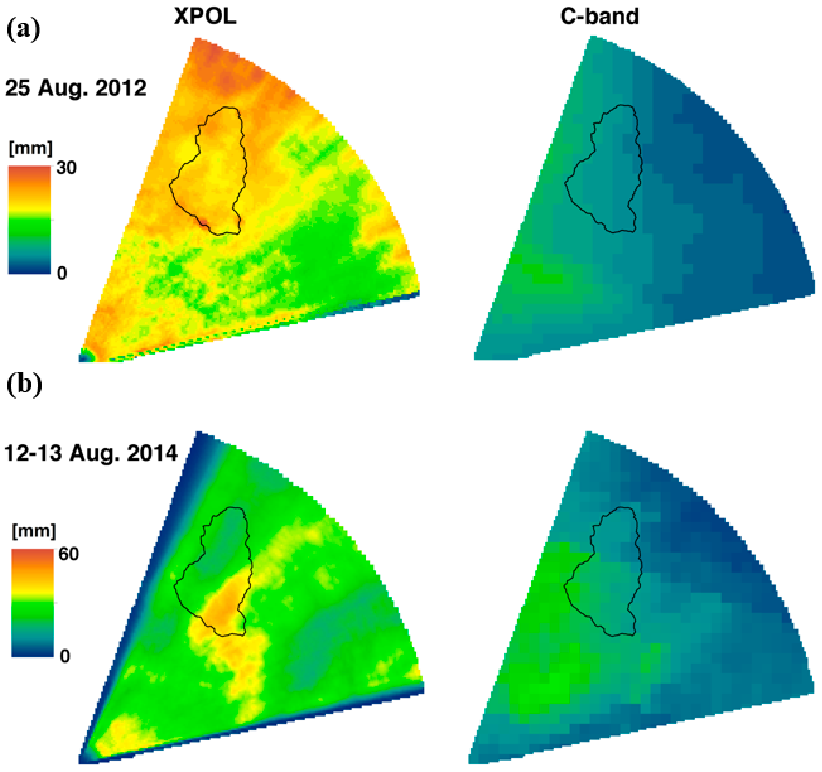
3.2. Case Study Analysis of Radar Rainfall Spatial Pattern

In this section, the evaluation of the radar rainfall estimates is performed qualitatively by comparing the spatial patterns of rain accumulation for the two rain events identified previously as the ones that caused considerable runoff response in Saldur basin. The first event occurred on the 25th of August, 2012 and is classified as convective type. It lasted less than 10 h and resulted in rainfall accumulations greater than 25 mm. The second event occurred over a 35-h period on 12–13th August 2014 and was stratiform (widespread) precipitation, with an embedded convection in the northeast direction of the storm, associated with a higher event total rainfall accumulation (~35 mm) within the study domain (Figure 9). These events are used to demonstrate the differences in representation of spatial rainfall patterns between the operational (C-band) radar-rainfall products, the short-range/high-resolution XPOL measurements, and rain gauges. Figure 9a,b exhibits distinct differences in terms of the rainfall patterns captured by the two radar-rainfall products. Rainfall fields observed by the C-band radar networks are significantly underestimated and spatially smoothed relative to the precipitation fields retrieved by XPOL measurements. Observations from the visual interpretation of Figure 9 are further supported by the Taylor diagram [69] shown in Figure 10, which is a graphical representation of the statistical relationship between the point (pixel) radar-rainfall estimates (i.e., XPOL and the two C-band radars) and the respective one of the reference (i.e., rain gauge rainfall observations). The similarity between the two fields of the figure is quantified in terms of their correlation, their centered root-mean-square difference (cRMSD) and the amplitude of their variations (represented by their standard deviations).
Note that the means of the fields are subtracted out before computing their second-order statistics so the diagram does not provide information about overall biases, but solely characterizes the centered pattern error. The position of each letter appearing on the plot quantifies how closely the radar precipitation estimates match the reference. The cRMSD between the observed and the reference patterns is proportional to the distance to the point on the x-axis identified as the reference “observation”. For both events, we note a low correlation for the operational C-band estimates and a significant underestimation of the reference standard deviation. For instance, for the 25th of August (Figure 10a) event the correlation coefficient of the XPOL estimates (both 200 and 1000 m resolution) are nearly 0.75 compare to the C-band estimates that have 0.35 (Figure 10a). The normalized RMSD (nRMSD) is also lower for the XPOL estimates. For the stratiform precipitation event of 12–13 August 2014 (Figure 10b), the XPOL estimates reveal higher correlations (~0.85) and lower RMSD values (close to 1.5). The C-band estimates also exhibit higher correlation (close to 0.7) and relative RMSD close to 1.8. The XPOL precipitation fields had standard deviations close to the reference rainfall fields, while the C-band precipitation estimates greatly underestimate the reference rainfall variability.

3.3. Hydrologic Evaluation of Radar-Rainfall Estimates

The potential benefit in using short-range X-band dual-polarization high-resolution observations for flood modeling applications in mountainous basins is examined by comparing the different radar and gauge-based hydrologic simulations, with the latter used as a reference throughout the hydrologic analysis. Runoff response in the study basin is simulated using a spatially distributed hydrologic model forced with rainfall estimates from the gauges, the operational radar, and the XPOL. The following sections discuss the selected runoff events, the hydrologic modeling setup and the analysis of simulated runoff.

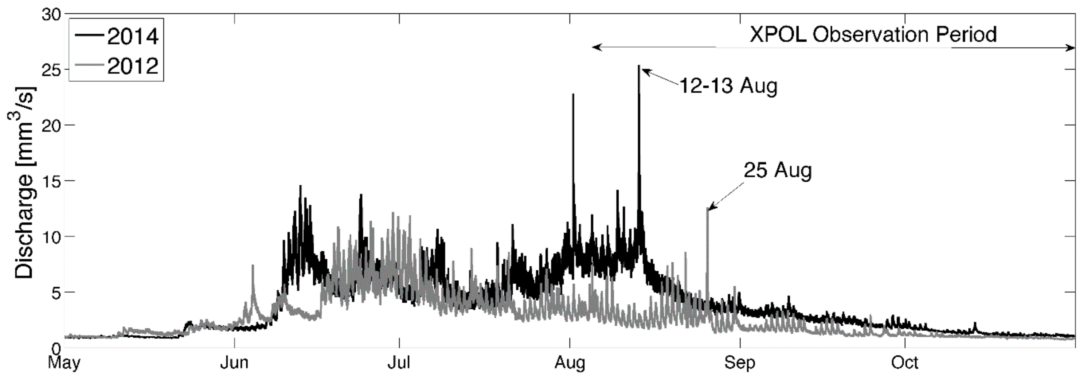
3.3.1. Runoff Events

The main volume of annual runoff in Saldur basin is generated between May and September, which is typical of snow dominated glaciated catchments. According to the tracer-based analysis of [50,66], the main runoff-contributing sources in the basin are as follows. From May to June, the runoff generation is predominantly attributed to melting of snow that has been accumulated during the cold season (late fall and winter). During mid-summer (July to early August), the runoff is largely generated by a mixture of snowmelt and glacier-melt and for the rest of the summer until September, glacier melt contributes to streamflow. At the same time, the precipitation events dominated by liquid phase (i.e., rainfall) translate in high direct runoff manifested as distinct spikes in runoff time series (Figure 11).
Since the focus of this study is on rainfall-runoff events, only the rainfall events associated with a significant signal in runoff response were selected for hydrologic analysis. From the list of events observed with XPOL (Table 1), only two events resulted in a considerable runoff response for the Saldur basin, which also corresponded to the annual max flow events of 2012 and 2014, respectively. The first event was during 25 August 2012 and was associated with an observed peak flow of ~12 m3 s−1 (at the basin outlet) and a gauge-based total basin-average rainfall of 21.2 mm. The second event on 13 August 2014 corresponded to an observed peak flow of ~25 m3 s−1 (Figure 11) and was associated with a 32.8 mm total basin-average rainfall. Note that those peak flow values correspond to the minimum and maximum of the annual max flows recorded within a 7-year record (2009–2014) of available discharge observations, respectively (stream gauges).
Based on the air temperatures of the Matsch LTER network, both events happened during a warm summer period. The snow limit was quite high (between 4500 and 3100 for the first one, between 3400 and 3100 for the second one), and therefore could be assumed that most of the basin was contributing by having liquid precipitation. On the basis of previous studies on the catchment, which analyzed the water sourced distribution along the season [70] and for specific events [51] we can estimate that in August roughly 50% of the base flow is due to glacier-melt, the snowmelt is negligible and the peak runoff is due to liquid precipitation.

3.3.2. Hydrologic Model Setup

The hydrologic simulations were carried out with a simple spatially distributed hydrologic model (KLEM—Kinematic Local Excess Model). The model is suitable for event-based rainfall-runoff analysis and has been used in several past studies in similar mountainous regions of northern Italy [71,72,73,74,75]. Model setup requires spatially distributed information of land surface properties (topography, soil type, and land use/cover) that were made available by the Hydrologic Office of the Autonomous Province of Bolzano. The model’s spatial resolution is dictated by the resolution of the digital elevation model, which in our case is 30 m. Runoff generation modelling is based on the Soil Conservation Service—Curve Number (SCS–CN) procedure [76]. Representation of runoff routing follows a simple scheme that distinguishes the drainage paths between the channel and hill slopes and assumes two spatially invariant velocities for hillslope and channel grids respectively [77]. The channel and hillslope grids are differentiated based on a channelization support area, which is considered constant at the sub-basin scale. For more information on KLEM model, the interested reader is referred to Reference [78] and references therein.
The model was calibrated to determine the required parameters that include the channelization support area, the channel and hillslope velocity, the parameter of infiltration storativity used in the SCS—CN procedure, and the parameter required for the specification of the initial abstraction [75]. Additionally, the identification of the appropriate antecedent moisture condition group required for CN calculation was also considered in the calibration exercise. Calibration of parameters was carried out manually for the rain gauge (reference) based simulations with the objective to achieve a realistic representation of the observed hydrograph shape and peak. Once calibrated, the model parameters were used consistently for the simulations based on XPOL and C-band rainfall estimates.
It is important to acknowledge that in a glaciated catchment, as our study basin, certain hydrological processes taking place such as glacier melting are not resolved by a relatively simple model like KLEM. However, implicitly accounting for their contribution (e.g., match antecedent flow conditions by proper initialization) permits the use of such a model to realistically simulate rainfall-to-runoff transformation at event scale. Given that the objective here is to examine the impact of differences in event rainfall (magnitude and spatial pattern) to runoff response, we consider that the application of KLEM is adequate for this purpose.

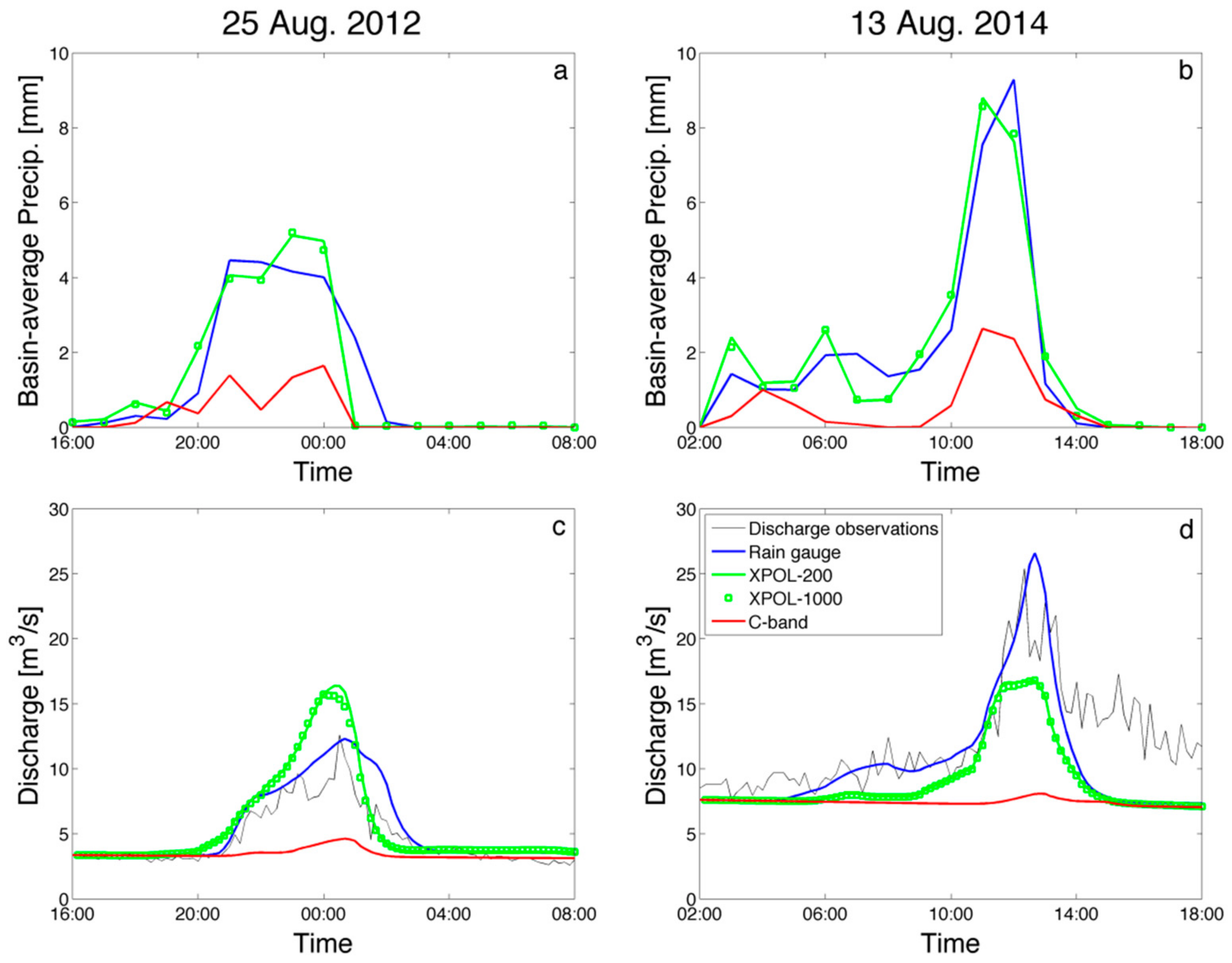
3.3.3. Simulation Results

Simulated runoff and basin-average rainfall, for the two events, are shown in Figure 12 for all the rainfall input scenarios examined (rain gauges, XPOL and C-band radars). The relative errors in the peak and total runoffs are summarized in Table 4.
The observed discharge time series are superimposed (Figure 12) to demonstrate the effectiveness of the hydrologic model’s calibration procedure, highlighting a good agreement in terms of peak runoff estimation. Comparison against the reference (control) runoff simulation is used in this study to evaluate the impact of radar-rainfall estimation uncertainty in rainfall-to-runoff transformation. One of the most distinct features revealed from the hydrologic simulations is that the C-band based simulated hydrographs showed almost no peak signature, revealing a dramatic underestimation of event flow peak in both cases examined. On the contrary, the XPOL-based simulations resulted in a clear flood hydrograph shape that quite well followed the dynamics of the reference-based simulations. However, it should be noted that XPOL-based simulations were associated with a considerable difference in the estimated hydrograph peak (27–37% with respect to gauge-based simulations) and inconsistent direction of the bias (i.e., underestimation or overestimation). Interestingly, comparison of the basin-average precipitation (Figure 12a,b) shows that the magnitude and dynamics are well captured by the XPOL estimates, which is why the relative difference in total runoff volume remains low (4–13%). This suggests that higher differences in the peak flow originate from differences in rainfall spatial pattern, which are further magnified due to the highly nonlinear propagation of errors from rainfall to peak flow.
The comparison of XPOL results at the two different grid resolutions (200 and 1000 m) shows that difference in pixel resolution did not have an important impact on the simulations of basin’s hydrologic response. This is somewhat expected, given previous research on the topic, which has shown that for the ratio of pixel resolution and basin scale considered here, no significant difference is expected in runoff response [11,79]. Overall, the findings from the hydrologic simulations demonstrate the potential benefit of using observations from locally deployed X-band dual-polarization radar for hydrological applications in mountainous areas. The systematic and severe underestimation in radar rainfall estimates from the regional C-band radar does not permit meaningful hydrologic analysis. This is also a clear indication of the potential limitations for using regional radars for developing flood early warning systems in remote complex terrain regions.

4. Conclusions

This study used data from a field experiment in the northeastern Italian Alps to demonstrate quantitative advantages from locally deployed dual-polarization X-band radar (XPOL) observations, relative to operational gauge-adjusted C-band radar-rainfall estimates, in terms of measuring rainfall over mountainous areas and the associated impacts in simulating runoff in small basins. The XPOL radar data were corrected for effects due to rain-path attenuation and the complex terrain (i.e., beam blockage, and VPR correction in areas with bright band and mixed phase contamination). For accurate calibration of radar parameters (ZH and ZDR), we used measurements from two disdrometers located at a site close to the radar with no intermediate obstacles. In addition, a three-dimensional model of the radar beam was applied to exclude highly occluded areas or to correct reflectivity from areas with minor occlusion (e.g., 3 dB reduction of ZH). Then polarimetric rainfall estimates were reported in two different spatial (200 and 1000 m) resolutions.
Ten rain events, measured by a locally deployed XPOL radar, dense in situ stations (rain gauges, disdrometers) and two regional operational radars, were selected to represent the case studies for this work. The intensity of the events was low to moderate, which did not induce significant flash flooding in the study area, but, according to the discharge observations, two of these events resulted in considerable direct runoff events. For the evaluation of radar-rainfall estimates, we selected fourteen different validation sites representing a large elevation range between 700 and 3500 m, which is not found in similar studies in the literature.
The comparison of the two XPOL spatial aggregation estimates with the in-situ gauges in both high and low elevations gave high correlations (0.60–0.99). The bias ratio for conditional (>0.1 mm h−1) and unconditional gauge rainfall varied between 20% and 53% overestimation. In two cases the total XPOL rainfall estimates exhibited two to three times larger precipitation accumulations than reference. No significant effect in the estimation accuracy was noted due to spatial resolution. The overall statistics showed better comparisons with the rain gauge measurements at high elevations (i.e., within the Saldur basin) and the XPOL rainfall estimation algorithm gave almost unbiased estimates for rainfall rates greater than 2 mm h−1. On the other hand, both the Austrian and Swiss operational radar network rainfall products gave lower correlations (0.45–0.85) against the in-situ gauges and high underestimation biases (from 0.21 up to 0.91 for the low elevation gauge groups, and from 0.24 up to 0.97 for the high elevation gauge groups).
Inspection of rainfall accumulation maps from the two high flow rainfall events showed that the spatial representation and magnitude of rainfall was significantly underestimated by the operational radar-rainfall products. Runoff simulations based on XPOL estimates were close to the reference (rain gauge) simulations in terms of runoff volume (relative difference <13%), but the peak runoff deviated by a larger degree (~30% relative difference). Simulations obtained from the operational radar rainfall products did not result in a notable peak flow. These results highlight the limitations of long-range radar observations for the flood modeling of small mountainous basins, and the potential from using locally deployed X-band radars as gap filling observing systems, especially in mountain regions, where beam blockage limits the effectiveness of traditional long-range C-band radars.
Even though the sample size associated with ten events was good enough to generate bulk error statistics in terms of precipitation estimation (mainly due to the number of in situ gauges), this study lacks a comprehensive representation of storm types, including rainfall intensities and high impact flood events. Therefore, it remains to be demonstrated how significant the described improvements are for different flood event severities and watershed characteristics, based on field experiments representing varying hydro-climatic regimes.

Author Contributions

M.N.A., J.K., M.B., E.N.A., E.M. and G.B. conceived and designed the experiments; M.N.A. and J.K. performed the XPOL and disdrometer experiments; M.B., E.M., U.T. and G.B. performed the ground validation rain gauge and discharge data and contribute on providing the Valluga and MeteoSwiss C-band radar data; M.N.A., J.K. and F.M. analyzed the precipitation data; E.I.N. carried out the hydrologic simulations and corresponding analysis and contributed the relevant text of the manuscript. E.N.A. contributed on the final revision of the paper; M.N.A. wrote the paper.

Funding

The research leading to these results has received part of the funding from the M. N. Anagnostou Postdoctoral Fellowship under the Action «Supporting Postdoctoral Researchers» of the Operational Program “Education and Lifelong Learning” (Action’s Beneficiary: General Secretariat for Research and Technology) and is co-financed by the European Social Fund (ESF) and the Greek State, under the Grand Agreement PE10 (975) HYDRO-X, coordinated by the National Observatory of Athens, Greece. In addition, EURAC activities were partially supported by the research projects “EMERGE: Retreating glaciers and emerging ecosystems in the Southern Alps” (Erich-Ritter-und Herzog-Sellenberg-Stiftung im Stifterverband für die Deutsche Wissenschaft) and “HydroAlp”, financed by Autonomous Province of Bolzano, Ripartizione Diritto allo Studio, Università e Ricerca Scientifica.

Acknowledgments

The authors would like to thank Urs Germann and Ioannis Sideris from MeteoSwiss for providing the Swiss Radar Network rainfall observations, and Andreas Schaffhauser (Austro Control Österreichische Gesellschaft, Austria) for providing the Valluga radar rainfall observations. Matteo Vischi and Pierpaolo Macconi (Ripartizione Opere Idrauliche, Provincia Autonoma di Bolzano—Italy) are thanked for the support in the installation of the XPOL radar. The study site is part of the LTSER Platform Matsch | Mazia, a member of the national and international Long-Term Ecological Research Networks (LTER-Italy, LTER-Europe and ILTER). Michael Engel and Francesco Comiti of the University of Bolzano are thanked for providing discharge and rainfall observations. G. Niedrist of EURAC is thanked for his work in maintaining the meteorological stations. Nikolopoulos acknowledges support from EU FP7 Marie Curie Actions IEF (project PIEF-GA-2011-302720).

Conflicts of Interest

The authors declare no conflict of interest.

References

  1. Petley, D. Global patterns of loss of life from landslides. Geology 2012, 40, 927–930. [Google Scholar] [CrossRef]
  2. Dowling, C.; Santi, P. Debris flows and their toll on human life: A global analysis of debris flow fatalities from 1950 to 2011. Nat. Hazards 2014, 71, 203–227. [Google Scholar] [CrossRef]
  3. Borga, M.; Stoffel, M.; Marchi, L.; Marra, F.; Jacob, M. Hydrogeomorphic response to extreme rainfall in headwater systems: Flash floods and debris flows. J. Hydrol. 2014, 518, 194–205. [Google Scholar] [CrossRef]
  4. Westra, S.; Fowler, H.J.; Evans, J.P.; Alexander, L.V.; Berg, P.; Johnson, F.; Kendon, E.J.; Lenderink, G.; Roberts, N.M. Future changes to the intensity and frequency of short-duration extreme rainfall. Rev. Geophys. 2014, 52, 522–555. [Google Scholar] [CrossRef] [Green Version]
  5. Molnar, P.; Fatichi, S.; Gaal, L.; Szolgay, J.; Burlando, P. Storm type effects on super Clausius-Clapeyron scaling of intense rainstorm properties with air temperature. Hydrol. Earth Syst. Sci. 2015, 19, 1753–1766. [Google Scholar] [CrossRef]
  6. UNISDR 2009. Terminology for Disaster Risk Reduction. Available online: http://www.unisdr.org/we/ inform/terminology (accessed on 11 January 2013).
  7. European Commission. Directive 2007/60/EC of the European Parliament and of the Council of 23 October 2007 on the Assessment and Management of Flood Risks; European Commission: Brussels, Belgium, 2007. [Google Scholar]
  8. Alfieri, L.; Salamon, P.; Pappenberger, F.; Wetterhall, F.; Thielen, J. Operational early warning systems for water-related hazards in Europe. Environ. Sci. Policy 2012, 21, 35–49. [Google Scholar] [CrossRef]
  9. Liechti, K.; Zappa, M.; Fundel, F.; Germann, U. Probabilistic evaluation of ensemble discharge nowcasts in two nested Alpine basins prone to flash floods. Hydrol. Process. 2013, 27, 5–17. [Google Scholar] [CrossRef]
  10. Zoccatelli, D.; Borga, M.; Zanon, F.; Antonescu, B.; Stancalie, G. Which Rainfall Spatial Information for Flash Flood Response Modelling? A Numerical Investigation Based on Data from the Carpathian Range, Romania. J. Hydrol. 2010, 394, 148–161. [Google Scholar] [CrossRef]
  11. Nikolopoulos, E.I.; Anagnostou, E.N.; Borga, M.; Vivoni, E.R.; Papadopoulos, A. Sensitivity of a mountain basin flash flood to initial wetness condition and rainfall variability. J. Hydrol. 2011, 402, 165–178. [Google Scholar] [CrossRef]
  12. Lobligeois, F.; Andréassian, V.; Perrin, C.; Tabary, P.; Loumagne, C. When does higher spatial resolution rainfall information improve streamflow simulation? An evaluation using 3620 flood events. Hydrol. Earth Syst. Sci. 2014, 18, 575–594. [Google Scholar] [CrossRef] [Green Version]
  13. Nikolopoulos, E.I.; Crema, S.; Marchi, L.; Marra, F.; Guzzetti, F.; Borga, M. Impact of uncertainty in rainfall estimation on the identification of rainfall thresholds for debris flow occurrence. Geomorphology 2014, 221, 286–297. [Google Scholar] [CrossRef]
  14. Marra, F.; Nikolopoulos, E.I.; Creutin, J.D.; Borga, M.; Creutin, J.D. Radar rainfall estimation for the identification of debris-flow occurrence thresholds. J. Hydrol. 2014, 519, 1607–1619. [Google Scholar] [CrossRef]
  15. Barros, A.P.; Joshi, M.; Putkonen, J.; Burbank, D.W. A study of the 1999 monsoon rainfall in a mountainous region in central Nepal using TRMM products and rain gauge observations. Geophys. Res. Lett. 2000, 27, 3683–3686. [Google Scholar] [CrossRef] [Green Version]
  16. Maddox, R.A.; Zhang, J.; Gourley, J.J.; Howard, K.W. Weather Radar Coverage over the Contiguous United States. Weather Forecast. 2002, 17, 927–934. [Google Scholar] [CrossRef]
  17. Lewis, H.W.; Harrison, D.L. Assessment of radar data quality in upland catchments. Meteorol. Appl. 2007, 14, 441–454. [Google Scholar] [CrossRef] [Green Version]
  18. Zhang, J.; Qi, Y.; Kingsmill, D.; Howard, K. Radar-Based Quantitative Precipitation Estimation for the Cool Season in Complex Terrain: Case Studies from the NOAA Hydrometeorology Testbed. J. Hydrometeorol. 2012, 13, 1836–1854. [Google Scholar] [CrossRef]
  19. White, A.B.; Neiman, P.J.; Ralph, F.M.; Kingsmill, D.E.; Persson, P.O.G. Coastal orographic rainfall processes observed by radar during the California landfalling jets experiment. J. Hydrometeorol. 2003, 4, 264–282. [Google Scholar] [CrossRef]
  20. Chen, S.; Gourley, J.J.; Hong, Y.; Kirstetter, P.E.; Zhang, J.; Howard, K.; Flamig, Z.L.; Hu, J.; Qi, Y. Evaluation and Uncertainty Estimation of NOAA/NSSL Next-Generation National Mosaic Quantitative Precipitation Estimation Product (Q2) over the Continental United States. J. Hydrometeorol. 2013, 14, 1308–1322. [Google Scholar] [CrossRef]
  21. Smith, J.A.; Miller, A.J.; Baeck, M.L.; Nelson, P.A.; Fisher, G.T.; Meierdiercks, K.L. Extraordinary flood response of a small urban watershed to short-duration convective rainfall. J. Hydrometeorol. 2005, 6, 599–617. [Google Scholar] [CrossRef]
  22. Anagnostou, M.N.; Kalogiros, J.; Anagnostou, E.N.; Papadopoulos, A. Experimental results on rainfall estimation in complex terrain with a mobile X-band polarimetric radar. Atmos. Res. 2009, 94, 579–595. [Google Scholar] [CrossRef]
  23. Anagnostou, M.N.; Kalogiros, J.; Anagnostou, E.N.; Tarolli, M.; Papadopoulos, A.; Borga, M. Performance evaluation of high-resolution rainfall estimation by X-band dual-polarization radar for flash flood applications in mountainous basin. J. Hydrol. 2010, 394, 4–16. [Google Scholar] [CrossRef]
  24. Wang, Y.; Chandrasekar, V. Quantitative precipitation estimation in the CASA X-band dual-polarization radar network. J. Atmos. Ocean. Technol. 2010, 27, 1665–1676. [Google Scholar] [CrossRef]
  25. Shakti, P.C.; Maki, M.; Shimizu, S.; Maesaka, T.; Kim, D.; Lee, D.; Iida, H. Correction of Reflectivity in the Presence of Partial Beam Blockage over a Mountainous Region Using X-Band Dual Polarization Radar. J. Hydrometeorol. 2013, 14, 744–764. [Google Scholar]
  26. Matrosov, S.Y.; Cifelli, R.; Gochis, D. Measurements of Heavy Convective Rainfall in the Presence of Hail in Flood-Prone Areas Using an X-Band Polarimetric Radar. J. Appl. Meteorol. Climatol. 2013, 52, 395–407. [Google Scholar] [CrossRef]
  27. Koffi, A.K.; Gosset, M.; Zahiri, E.-P.; Ochou, A.D.; Kacou, M.; Cazenave, F.; Assamoi, P. Evaluation of X-band polarimetric radar estimation of rainfall and rain drop size distribution parameters in West Africa. Atmos. Res. 2014, 143, 438–461. [Google Scholar] [CrossRef]
  28. Vulpiani, G.; Baldini, L.; Roberto, N. Characterization of Mediterranean hail-bearing storms using an operational polarimetric X-band radar. Atmos. Meas. Tech. 2015, 8, 4681–4698. [Google Scholar] [CrossRef] [Green Version]
  29. Marra, F.; Morin, E. Autocorrelation structure of convective rainfall in semiarid-arid climate derived from high-resolution X-band radar estimates. Atmos. Res. 2018, 200, 126–138. [Google Scholar] [CrossRef]
  30. Chandrasekar, V.; Wang, Y.; Maki, M.; Nakane, K. Flood Monitoring using X-band Dual-polarization Radar Network. In Proceedings of the 11th Plinius Conference on Mediterranean Storms, Barcelona, Spain, 7–10 September 2009. [Google Scholar]
  31. Matrosov, S.Y.; Clark, A.; Martner, B.E.; Tokay, A. X-band polarimetric radar measurements of rainfall. J. Appl. Meteorol. 2002, 41, 941–952. [Google Scholar] [CrossRef]
  32. Anagnostou, E.N.; Anagnostou, M.N.; Krajewski, W.F.; Kruger, A.; Miriovsky, B.J. High-resolution rainfall estimation from X-band polarimetric radar measurements. J. Hydrometeorol. 2004, 5, 110–128. [Google Scholar] [CrossRef]
  33. Park, S.-G.; Maki, M.; Iwanami, K.; Bringi, V.N.; Chandrasekar, V. Correction of Radar Reflectivity and Differential Reflectivity for Rain Attenuation at X Band. Part I: Theoretical and Empirical Basis. J. Atmos. Ocean. Technol. 2005, 22, 1621–1632. [Google Scholar] [CrossRef] [Green Version]
  34. Kim, D.-S.; Maki, M.; Lee, D.-I. Retrieval of three dimensional raindrop size distribution using X-band polarimetric radar. J. Atmos. Ocean. Technol. 2010, 27, 1265–1285. [Google Scholar] [CrossRef]
  35. Kalogiros, J.; Anagnostou, M.N.; Anagnostou, E.N.; Montopoli, M.; Picciotti, E.; Marzano, F.S. Correction of Polarimetric Radar Reflectivity Measurements and Rainfall Estimates for Apparent Vertical Profile in Stratiform Rain. J. Appl. Meteorol. Climatol. 2013, 52, 1170–1186. [Google Scholar] [CrossRef]
  36. Kalogiros, J.; Anagnostou, M.N.; Anagnostou, E.N.; Montopoli, M.; Picciotti, E.; Marzano, F.S. Optimum estimation of rain microphysical parameters using X-band dual-polarization radar observables. IEEE Trans. Geosci. Remote Sens. 2013, 51, 3063–3076. [Google Scholar] [CrossRef]
  37. Anagnostou, M.N.; Kalogiros, J.; Marzano, F.S.; Anagnostou, E.N.; Montopoli, M.; Picciotti, E. Performance evaluation of a new dual-polarization microphysical algorithm based on long-term X-band radar and disdrometer observations. J. Hydrometeorol. 2013, 14, 560–576. [Google Scholar] [CrossRef]
  38. Lim, S.; Cifelli, R.; Chandrasekar, V.; Matrosov, S.Y. Precipitation Classification and Quantification Using X-Band Dual-Polarization Weather Radar: Application in the Hydrometeorology Testbed. J. Atmos. Ocean. Technol. 2013, 30, 2108–2120. [Google Scholar] [CrossRef]
  39. Chang, W.-Y.; Vivekanandan, J.; Wang, T.-C.C. Estimation of X-Band Polarimetric Radar Attenuation and Measurement Uncertainty Using a Variational Method. J. Appl. Meteorol. Climatol. 2014, 53, 1099–1119. [Google Scholar] [CrossRef]
  40. Thurai, M.; Mishra, K.V.; Bringi, V.N.; Krajewski, W.F. Initial Results of a New Composite-Weighted Algorithm for Dual-Polarized X-band Rainfall Estimation. J. Hydrometeorol. 2017, 18, 1081–1100. [Google Scholar] [CrossRef]
  41. Matrosov, S.Y.; Kingsmill, D.E.; Martner, B.E.; Ralph, F.M. The utility of X-band polarimetric radar for quantitative estimates of rainfall parameters. J. Hydrometeorol. 2005, 6, 248–262. [Google Scholar] [CrossRef]
  42. Chen, H.; Chandrasekar, V. The Quantitative Precipitation Estimation System for Dallas-Fort Worth (DFW) Urban Remote Sensing Network. J. Hydrol. 2015, 531 Pt 2, 259–271. [Google Scholar] [CrossRef]
  43. Yang, W.-Y.; Ni, G.-H.; Qi, Y.-C.; Hong, Y.; Sun, T. Exploring the potential of utilizing high resolution X-band radar for urban rainfall estimation. Atmos. Meas. Tech. Discuss. 2016. [Google Scholar] [CrossRef]
  44. Chandrasekar, V.; Wang, Y.; Chen, H. The CASA quantitative precipitation estimation system: A five year validation study. Nat. Hazards Earth Syst. Sci. 2012, 12, 2811–2820. [Google Scholar] [CrossRef]
  45. Cifelli, R.; Chandrasekar, V.; Chen, H.; Johnson, L.E. High resolution radar quantitative precipitation estimation in the San Francisco Bay Area: Rainfall monitoring for the urban environment. J. Meteorol. Soc. Jpn. 2018, 96A. [Google Scholar] [CrossRef]
  46. Mishra, K.V.; Krajewski, W.F.; Goska, R.; Ceynar, D.; Seo, B.-C.; Kruger, A.; Niemeier, J.J.; Galvez, M.B.; Thurai, M.; Bringi, V.N.; et al. Deployment and Performance Analyses of High-Resolution Iowa XPOL Radar System during the NASA IFloodS Campaign. J. Hydrometeorol. 2016, 17, 455–479. [Google Scholar] [CrossRef]
  47. Lim, S.; Lee, D.-R.; Cifelli, R.; Hwang, S.H. Quantitative precipitation estimation for an X-band dual-polarization radar in the complex mountainous terrain. KSCE J. Civ. Eng. 2014, 18, 1548–1553. [Google Scholar] [CrossRef]
  48. Paschalis, A.; Fatichi, S.; Molnar, P.; Rimkus, S.; Burlando, P. On the effects of small scale space-time variability of rainfall on basin flood response. J. Hydrol. 2014, 514, 313–327. [Google Scholar] [CrossRef]
  49. Comiti, F.; Marchi, L.; Macconi, P.; Arattano, M.; Bertoldi, G.; Borga, M.; Brardinoni, F.; Cavalli, M.; D’Agostino, V.; Penna, D.; et al. A new monitoring station for debris flows in the European Alps: First observations in the Gadria basin. Nat. Hazards 2014, 73, 1175–1198. [Google Scholar] [CrossRef]
  50. Mao, L.; Dell’Agnese, A.; Huincache, C.; Penna, D.; Engel, M.; Niedrist, G.; Comiti, F. Bedload hysteresis in a glacier-fed mountain river. Earth Surf. Process. Landf. 2015, 39, 964–976. [Google Scholar] [CrossRef]
  51. Engel, M.; Penna, D.; Bertoldi, G.; Dell’Agnese, A.; Soulsby, C.; Comiti, F. Identifying run-off contributions during melt-induced run-off events in a glacierized alpine catchment. Hydrol. Process. 2016, 30, 343–364. [Google Scholar] [CrossRef]
  52. Galos, S.; Kaser, G. The Mass Balance of Matscherferner 2012/13, Project Report; University of Innsbruck: Innsbruck, Austria, 2014. [Google Scholar]
  53. Engel, M.; Notarnicola, C.; Endrizzi, S.; Bertoldi, G. Snow model sensitivity analysis to understand spatial and temporal snow dynamics in a high-elevation catchment. Hydrol. Process. 2017, 31, 4151–4168. [Google Scholar] [CrossRef]
  54. Penna, D.; Engel, M.; Mao, L.; Dell’Agnese, A.; Bertoldi, G.; Comiti, F. Tracer-based analysis of spatial and temporal variation of water sources in a glacierized catchment. Hydrol. Earth Syst. Sci. 2014, 18, 5271–5288. [Google Scholar] [CrossRef]
  55. Bertoldi, G.; Della Chiesa, S.; Notarnicola, C.; Pasolli, L.; Niedrist, G.; Tappeiner, U. Estimation of soil moisture patterns in mountain grasslands by means of SAR RADARSAT 2 images and hydrological modelling. J. Hydrol. 2014, 516, 245–257. [Google Scholar] [CrossRef]
  56. Mair, E.; Leitinger, G.; della Chiesa, S.; Niedrist, G.; Tappeiner, U.; Bertoldi, G. A simple method to combine snow height and meteorological observations to estimate winter precipitation at sub-daily resolution. Hydrol. Sci. J. 2015, 61, 2050–2060. [Google Scholar] [CrossRef]
  57. Schaffhauser, A.; Auer, M.; Kann, A. Weather Radar Observations at high altitude is it worth the effort? In Proceedings of the 6th European Conference on Radar in Meteorology and Hydrology (ERAD), Sibiu, Romania, 6–10 September 2010. [Google Scholar]
  58. Paulitsch, H.; Teschl, F.; Randeu, W.L. Dual-polarization C-band weather radar algorithms for rain rate estimation and hydrometeor classification in an alpine region. Adv. Geosci. 2009, 20, 3–8. [Google Scholar] [CrossRef]
  59. Paulitsch, H.; Teschl, F.; Randeu, W.L. Preliminary evaluation of polarimetric parameters from a new dual-polarization C-band weather radar in an alpine region. Adv. Geosci. 2010, 25, 111–117. [Google Scholar] [CrossRef] [Green Version]
  60. Germann, U.; Galli, G.; Boscacci, M.; Bolliger, M. Radar precipitation measurement in a mountainous region. Q. J. R. Meteorol. Soc. 2006, 132, 1669–1692. [Google Scholar] [CrossRef] [Green Version]
  61. Sideris, I.; Gabella, M.; Sassi, M.; Germann, U. Real-time spatiotemporal merging of radar and raingauge precipitation measurements in Switzerland. In Proceedings of the 9th International Workshop on Precipitation in Urban Areas, Urban Challenges in Rainfall Analysis, St. Moritz, Switzerland, 6–9 December 2012. [Google Scholar]
  62. Sideris, I.; Gabella, M.; Erdin, R.; Germann, U. Real-time radar-raingauge merging using spatio-temporal co-kriging with external drift in the Alpine terrain of Switzerland. Q. J. R. Meteorol. Soc. 2014, 140, 1097–1111. [Google Scholar] [CrossRef]
  63. Sideris, I.; Gabella, M.; Sassi, M.; Germann, U. The CombiPrecip experience: Development and operation of a real-time radar-raingauge combination scheme in Switzerland. In Proceedings of the 9th Weather Radar and Hydrology (WRaH) International Symposium, Washington, DC, USA, 7–9 April 2014. [Google Scholar]
  64. Kalogiros, J.; Anagnostou, M.N.; Anagnostou, E.N.; Montopoli, M.; Picciotti, E.; Marzano, F.S. Evaluation of a new Polarimetric Algorithm for Rain-Path Attenuation Correction of X-Band Radar Observations Against Disdrometer Data. IEEE Geosci. Remote Sens. Lett. 2014, 52, 1369–1380. [Google Scholar] [CrossRef]
  65. Testud, J.; le Bouar, E.; Obligis, E.; Ali-Mehenni, M. The rain profiling algorithm applied to polarimetric weather radar. J. Atmos. Ocean. Technol. 2000, 17, 332–356. [Google Scholar] [CrossRef]
  66. Gorgucci, E.; Chandrasekar, V.; Baldini, L. Correction of X-band radar observation for propagation effects based on the self-consistency principle. J. Atmos. Ocean. Technol. 2006, 23, 1668–1681. [Google Scholar] [CrossRef]
  67. Matrosov, S.Y.; Kurt, C.; Kingsmill, A.; David, E. A polarimetric radar approach to identify rain. Melting-layer and snow regions for applying corrections to vertical profiles of reflectivity. J. Appl. Meteorol. Climatol. 2007, 46, 154–166. [Google Scholar] [CrossRef]
  68. Borga, M.; Anagnostou, E.N.; Frank, E. On the use of real-time radar rainfall estimates for flood prediction in mountainous basins. J. Geophys. Res. Atmos. 2000, 105, 2269–2280. [Google Scholar] [CrossRef] [Green Version]
  69. Taylor, K.E. Summarizing multiple aspects of model performance in a single diagram. J. Geophys. Res. 2001, 106, 7183–7192. [Google Scholar] [CrossRef] [Green Version]
  70. Penna, D.; Engel, M.; Bertoldi, G.; Comiti, F. Towards a tracer-based conceptualization of meltwater dynamics and streamflow response in a glacierized catchment. Hydrol. Earth Syst. Sci. 2017, 21, 23–41. [Google Scholar] [CrossRef] [Green Version]
  71. Sangati, M.; Borga, M.; Rabuffetti, D.; Bechini, R. Influence of rainfall and soil properties spatial aggregation on extreme flash flood response modelling: An evaluation based on the Sesia river basin, North Western Italy. Adv. Water Res. 2009, 32, 1090–1106. [Google Scholar] [CrossRef]
  72. Zoccatelli, D.; Borga, M.; Viglione, A.; Chirico, G.B.; Blöschl, G. Spatial moments of catchment rainfall: Rainfall spatial organisation, basin morphology, and flood response. Hydrol. Earth Syst. Sci. 2011, 15, 3767–3783. [Google Scholar] [CrossRef] [Green Version]
  73. Nikolopoulos, E.I.; Borga, M.; Zoccatelli, D.; Anagnostou, E.N. Catchment-Scale Storm Velocity: Quantification, Scale Dependence and Effect on Flood Response. Hydrol. Sci. J. 2014, 59, 1363–1376. [Google Scholar] [CrossRef]
  74. Bartsotas, N.S.; Nikolopoulos, E.I.; Anagnostou, E.N.; Solomos, S.; Kallos, G. Moving Toward Subkilometer Modeling Grid Spacings: Impacts on Atmospheric and Hydrological Simulations of Extreme Flash Flood-Inducing Storms. J. Hydrol. 2017, 18, 209–226. [Google Scholar] [CrossRef]
  75. Destro, E.; Amponsah, W.; Nikolopoulos, E.I.; Marchi, L.; Marra, F.; Zoccatelli, D.; Borga, M. Coupled prediction of flash flood response and debris flow occurrence: Application on an alpine extreme flood event. J. Hydrol. 2018, 558, 225–237. [Google Scholar] [CrossRef]
  76. U.S. Department of Agriculture. Urban Hydrology for Small Watersheds; Technical Release; U.S. Department of Agriculture: Washington, DC, USA; Volume 55, p. 164.
  77. Da Ros, D.; Borga, M. Use of digital elevation model data for the derivation of the geomorphological instantaneous unit hydrograph. Hydrol. Process. 1997, 11, 13–33. [Google Scholar] [CrossRef]
  78. Borga, M.; Boscolo, P.; Zanon, F.; Sangati, M. Hydrometeorological Analysis of the 29 August 2003 Flash Flood in the Eastern Italian Alps. J. Hydrometeorol. 2007, 8, 1049–1067. [Google Scholar] [CrossRef]
  79. Sangati, M.; Borga, M. Influence of rainfall spatial resolution on flash flood modeling. Nat. Hazards Earth Syst. Sci. 2009, 9, 575–584. [Google Scholar] [CrossRef]
Figure 1. The topography of the experimental area showing the coverage of the XPOL radar encompassing the experimental basin, the various in situ instruments, and the coverage of the two operational network radars. Pictures from the deployed sensors are also shown (at the lower right is the XPOL radar, in the middle are two NOA gauges and the 2D-video disdrometer and at the top are the Parsivel disdrometer and Micro-Rain-Radar of NASA).
Remotesensing 10 01258 g001
Figure 2. The scatter plots between the calibrated radar reflectivity ZhR and differential reflectivity ZdrR at the position of the disdrometers (0.5° elevation angle of the radar antenna) and the corresponding reflectivities (ZhD and ZdrD) estimated from the disdrometers for (a) 2012 and (b) 2014 observations.
Remotesensing 10 01258 g002
Figure 3. The application of the VPR correction algorithm to XPOL data at (a) 1.5° and (b,c) 3.5° elevation and comparison with in situ (2DVD and Parsivel) data on 24 September 2012.
Remotesensing 10 01258 g003
Figure 4. The same as Figure 3, but for the rain events of 12–13 and 9 August 2014 at (a) 1.5° and (b,c) 3.5°.
Remotesensing 10 01258 g004
Figure 5. The PPI plots of accumulated rain estimated by the XPOL radar before (a,b) and after the VPR correction (c,d) at elevations 2.5° (a,c) and 3.5° (b,d) for the rain event of 24 September 2012.
Remotesensing 10 01258 g005
Figure 6. The same as Figure 5 but for the rain event of 12 August 2014, before (a,b) and after the VPR correction (c,d) at elevations 2.5° (a,c) and 3.5° (b,d).
Remotesensing 10 01258 g006
Figure 7. The scatter plots of rainfall rate, estimated from the radar (at the 1.5° elevation) without (light grey dots) and with VPR (black dots) correction against in situ measurements for the rain events of (a,b) 2012 and (c) 2014.
Remotesensing 10 01258 g007
Figure 8. The scatter plots between the hourly rainfall estimation of XPOL and the large operational network radars versus the ground validation in situ sites separated into low and high elevation (inside the Saldur basin) gauge groups. The black line is the ‘1-1’ relation.
Remotesensing 10 01258 g008
Figure 9. The storm total accumulation estimation maps (in mm) during the (a) 25 August 2012 and (b) the 12–13 August 2014 of Swiss network operation radar estimates (on the right panel) and XPOL estimates (on the left panels).
Remotesensing 10 01258 g009
Figure 10. The Taylor diagram displaying a statistical comparison of three different daily accumulation radar precipitation estimates with in situ observations. The azimuthal angle represents correlation; the radial distance, the standard deviation; and the semicircles centered at the “observation” marker, the standard deviation of the errors. (a) 25 August 2012; (b) 12–13 August 2014.
Remotesensing 10 01258 g010
Figure 11. The time series of observed and discharge at the outlet of Saldur basin. The XPOL observation period and the two events analyzed are noted on the graph.
Remotesensing 10 01258 g011
Figure 12. The time series of the basin: the average precipitation (top) and simulated discharge (bottom) at Saldur outlet (WG1) during 25 August (left) and 13 August (right), according to rain gauges (blue), XPOL-200 m (green), XPOL-1 km (green squares) and C-band (red) estimates. Available discharge measurements (thin black) are also shown.
Remotesensing 10 01258 g012
Table 1. The technical specifications of the three C-band radars from for MeteoSwiss network and the Valluga radar of the Austrian weather radar operational network.
1. Swiss Radars2. Valluga Radar
Operating FrequencyC-band (5.4 GHz)C-band (5.625 GHz)
Pulse Length0.5 μs0.8 μs
PRFvariable from 600 to 1500 Hz1000 Hz
PolarizationDualDual
Dynamic Range105 dB108 dB
Max Range246 km120
Angular Resolution1° with 20 elevations per 5 min1° with 14 elevations per 5 min
Range Resolution83 m125 m
Beamwidth~1°~0.92°
Table 2. The selected rain events for the two observations periods in 2012 and 2014. In this table, “Total average—gauge rain indicates the surface basin total (for the time period) average rainfall”.
Time Period (UTC)
(day/month/year)
Total Average–Gauge Rain (mm)Available Observations
06/08/12 17:00–06/08/12 21:0010Rain gauges (all sites), 2DVD, Parsivel, XPOL, Valluga
25/08/12 16:00–25/08/12 24:0021Rain gauges (all sites), Parsivel, XPOL, Swiss Radar Network
10/09/12 08:00–12/09/12 21:0016Rain gauges (all sites), 2DVD, Parsivel, MRR, XPOL, Valluga
24/09/12 07:00–27/09/12 21:3028Rain gauges (all sites), 2DVD, Parsivel, MRR, XPOL, Valluga
29/09/12 07:00–30/09/12 06:3011Rain gauges (all sites), 2DVD, Parsivel, MRR, XPOL, Valluga
04/08/14 15:00–05/08/14 04:0011Rain gauges (all sites), Parsivel, XPOL, Swiss Radar Network
09/08/14 08:00–09/08/14 15:0014Rain gauges (all sites), Parsivel, XPOL, Swiss Radar Network
12/08/14 06:00–13/08/14 22:0037Rain gauges (all sites), Parsivel, XPOL, Swiss Radar Network
29/08/14 20:00–01/09/14 08:0010Rain gauges (all sites), Parsivel, XPOL, Swiss Radar Network
15/09/14 14:00–16/09/14 23:0013Rain gauges (all sites), Parsivel, XPOL, Swiss Radar Network
Table 3. The statistical evaluation of the radar rainfall products; statistics in parenthesis represents the “low-elevation” reference in situ inside the Saldur basin.
CorrelationConditional BiasUnconditional Bias
Date/Radar
(dd/mm/yy)
C-BandsXPOL-200 mXPOL-1000 mC-BandsXPOL-200 mXPOL-1000 mC-BandsXPOL-200 mXPOL-1000 m
06/08/120.65 (0.65)0.82 (0.97)0.83 (0.95)0.69 (0.51)0.95 (1.02)0.93 (1.04)0.37 (0.49)1.26 (1.24)1.22 (1.20)
25/08/120.69 (0.75)0.89 (0.84)0.89 (0.83)0.32 (0,19)1.11 (1.19)1.12 (1.18)0.27 (0.21)1.08 (1.22)1.10 (1.21)
10/09/120.71 (0.69)0.68 (0.90)0.70 (0.91)0.35 (0.21)0.77 (1.02)0.77 (0.99)0.35 (0.24)0.81 (1.09)0.82 (1.12)
24/09/120.68 (0.67)0.94 (0.99)0.91 (0.98)0.34 (0.40)1.06 (1.03)1.09 (1.03)0.24 (0.31)1.08 (1.05)1.11 (1.07)
29/09/120.43 (0.51)0.82 (0.95)0.81 (0.95)0.91 (0.37)0.98 (0.91)1.01 (0.89)0.34 (0.32)1.16 (1.18)1.18 (1.21)
04/08/140.53 (0.56)0.94 (0.88)0.93 (0.83)1,96 (2.08)0.71 (0.99)0.67 (1.11)1.96 (2.13)0.76 (0.99)0.71 (1.11)
09/08/140.69 (0.68)0.83 (0.92)0.77 (0.86)0.72 (0.84)0.74 (1.01)0.68 (1.07)0.75 (0.97)0.74 (1.03)0.68 (1.06)
12/08/140.68 (0.71)0.81 (0.91)0.80 (0.85)0.58 (0.91)1.17 (0.99)1.31 (0.97)0.58 (1.03)1.21 (1.01)1.35 (0.96)
29/08/140.52 (0.57)0.62 (0.70)0.54 (0.60)0.70 (0.84)1.69 (1.60)2.06 (2.14)0.68 (0.79)2.01 (1.91)2.40 (2.43)
15/09/140.66 (0.88)0.83 (0.93)0.77 (0.58)2.38 (0.45)2.52 (1.34)2.81 (1.89)2.50 (0.45)2.71 (1.56)3.10 (2.06)
Table 4. The basin-average rainfall accumulation and the relative difference in runoff peak and volume between the rain gauge and radar-based simulations for the two events of 25 August 2012 and 12–13 August 2014.
25 August 201212–13 August 2014
Total Rainfall (mm)Rel. Diff. in Peak Runoff (%)Rel. Diff. in Runoff Volume (%)Total Rainfall (mm)Rel. Diff. in Peak Flow (%)Rel. Diff. in Flow Volume (%)
Rain gauge21.2--32.8--
XPOL-20021.8334.436.4−37−12.7
XPOL-100021.727.83.835.8−37−13
C-band6−62.4−35.78.8−70−21.7

