Improving Geometric Performance for Imagery Captured by Non-Cartographic Optical Satellite: A Case Study of GF-1 WFV Imagery


1
State Key Laboratory of Information Engineering in Surveying, Mapping and Remote Sensing, Wuhan University, Wuhan 430079, China
2
Collaborative Innovation Center of Geospatial Technology, Wuhan University, Wuhan 430079, China
3
School of Remote Sensing and Information Engineering, Wuhan University, Wuhan 430079, China
4
China Academy of Space Technology, Beijing 100094, China
*
Author to whom correspondence should be addressed.
Remote Sens. 2018, 10(6), 971; https://doi.org/10.3390/rs10060971
Submission received: 14 May 2018
/
Revised: 8 June 2018
/
Accepted: 13 June 2018
/
Published: 18 June 2018
(This article belongs to the Section Remote Sensing Image Processing)
Abstract
:Numerous countries have established their own Earth observing systems (EOSs) for global change research. Data acquisition efforts are generally only concerned with the completion of the mission regardless of the potential to expand into other areas, which reduces the application effectiveness of Earth observation data. This paper explores the cartographic possibility of images being not initially intended for surveying and mapping, and a novel method is proposed to improve the geometric performance. First, the rigorous sensor model (RSM) is recovered from the rational function model (RFM), and then the system errors of the non-cartographic satellite’s imagery are compensated by using the conventional geometric calibration method based on RSM; finally, a new and improved RFM is generated. The advantage of the method over traditional ones is that it divides the errors into static errors and non-static errors for each image during the improvement process. Experiments using images collected with the Gaofen-1 (GF-1) wide-field view (WFV) camera demonstrate that the orientation accuracy of the proposed method is within 1 pixel for both calibration and validation images, and the obvious high-order system errors are eliminated. Moreover, a block adjustment test shows that the vertical accuracy is improved from 21 m to 11 m with four ground control points (GCPs) after compensation, which can fulfill requirements for 1:100,000 stereo mapping in mountainous areas. Generally, the proposed method can effectively improve the geometric potential for images captured by non-cartographic satellite.
1. Introduction
Numerous countries have established their own Earth observing systems (EOSs). For example, China has been working on the establishment of the meteorological Fengyun (FY) satellite series, oceanic Haiyang (HY) satellite series, Earth resource Ziyuan (ZY) satellite series [1,2], Environment and Disaster Monitoring Huanjing (HJ) satellite series, and China High-resolution Earth Observation System (CHEOS) [3,4]. The United States has developed an EOS plan [5], Earth Science Business Plan (ESE), and Integrated Earth Observation System (IEOS) [6], and it has launched numerous satellites including Landsat, Terra, Earth Observing-1 (EO-1), and other satellites [7]. Other countries such as Russia [8], Japan [9], Canada [10] and India [11] have also put forward corresponding Earth observation plans. Simultaneously, various commercial satellite companies have launched many influential commercial remote-sensing satellites including IKONOS [12,13], GeoEye-1 [14], QuickBird [15], WorldView 1/2 [16,17], SPOT6/7 [18], PLÉIADES 1A/B [19], and JL-1 [20]. On the basis of the implementation of these various types of Earth observation programs and the development of commercial remote-sensing satellites, Earth observation data have accumulated, especially optical remote-sensing data. These data have laid a solid foundation for global change research, and presently, there are various proposed methods and product specifications for such data.
With regard to satellites and the post-processing of image data, the corresponding Earth observation data-processing methods are generally designed according to the requirements of the mission. Because of the specifics of the mission, the acquired data is generally only concerned with the completion of the mission regardless of the ability to expand in other areas. For example, images of land and resources are rarely used for surveying and mapping, which has reduced the application benefits of Earth observation data to some extent. The cartographic possibility of using satellite imagery being not initially intended for surveying and mapping (non- cartographic satellite imagery) deserves exploration, as this could not only make up for the low quantity of surveying and mapping data but also improve the application effectiveness of Earth observation data. However, given that there are high requirements for interior accuracy during surveying and mapping, it will be crucial to detect and compensate for system errors, which have been barely considered in other fields when imagery captured by non-cartographic satellites were used.
Bias compensation methods (BCMs) have been studied and widely applied to compensate for satellite image errors, and these methods can generally be grouped into the shift model, the shift and drift model, the affine model, and the polynomial model. The shift model adds constant offsets directly in the image or object space and is effective for IKONOS [21], GeoEye-1, and WorldView-2 [22]. The shift and drift model is based on the shift model and adds a scale coefficient to compensate for the variation of the attitude errors caused by the drift of the satellite gyro with time. This model can be used to obtain relatively high compensation accuracy for QuickBird data [15]. The affine model is more commonly used, and it compensates for translation, scaling, rotation and shear deformation both in the image space and object space. Various verification studies have shown that the affine model is widely applicable to the IKONOS [23], QuickBird [24], WorldView [25], ALOS [26], ZY3 [1], and TH-1 [27] satellites. When multi-view and multi-track images are involved, the affine model can also be applied as a basic model for rational function model (RFM) block adjustments. In addition, the polynomial model can be used to achieve a compensation effect by establishing a high-order function for the residuals, which involves the use of low-order terms to model exterior element errors and high-order terms to model interior element errors. This kind of model has been adopted for error compensation and has shown good results in many studies [24,28,29]. Although BCMs are widely adopted, the following problems still arise during practical applications.
(1) The traditional BCMs for basic remote-sensing products are based on the RFM, which is used to establish an additional parameter model in the image space or the object space. No matter how complex the additional parameter model, the essence of the additional parameter model is to fit or approximate the residuals from the results and to perform corrections on the RFM based on additional parameters. Most methods can only achieve compensation for the exterior element errors after sufficient interior calibration work and will not work when images with interior element errors are provided. Although the polynomial model can partially compensate for interior errors in the image space, it requires a sufficient number of ground control points (GCPs) for each image and is not practically feasible.
(2) The systematic error in the traditional BCMs is defined as the integrated error (which includes the linear offset and non-linear offset) that leads to the systematic deviation of the current image. Essentially this includes the measurement errors of the ephemeris and attitude, installation error, and internal orientation element error. These errors are not differentiated and only considered within one image. In fact, the installation error and internal orientation element error are the same for each image. However, it should be noted that conventional methods fail to consider the stability of the installation error and interior orientation element error and compensate for these errors together with the orbit and attitude errors in the same image, which will inevitably cause many unnecessary calculations because compensation parameters for any image are different and, thus, control data are required separately for each image.
In addition to the BCMs, some researchers have proposed other methods. Xiong [30] proposed a generic processing method that recovers the rigorous sensor model (RSM) first and then adds constant compensation parameters to the recovered attitude and orbit data. Experiments proved that this method can obtain more robust results. Furthermore, this method was applied to block adjustments of IKONOS and QuickBird and yielded a sub-meter positioning accuracy. However, this method does not include a very clear procedure for recovering the RSM and fails to consider the stability of the interior elements error but calculates the compensated parameters and compensates for these errors together with the satellite position and attitude errors in the same imagery. In addition, Hu et al. [31] proposed a method for correcting the RFM parameters directly through additional control points, that is, by directly adding control point information into a constructed virtual control grid and by assigning certain weights to improve the accuracy of RFM but actually not performing any analysis and modeling of the system errors; the method was verified preliminarily with IKONOS data.
Considering the defects in the traditional methods, a novel method is proposed here for improving the geometric quality of a non-cartographic satellite’s images. First, the RSM is recovered from the RFM and then the system errors of non-cartographic satellite’s imagery can be compensated for by using the conventional geometric calibration method based on the RSM; finally, improved RFM is described. Its advantage over traditional methods is that the proposed method divides the errors into static errors (installation angle and interior orientation elements) and non-static errors (measurement errors of ephemeris and attitude) for each image during the improvement process. Besides, the multi-GCF strategy is proposed to solve the problem that requires a solution of compensation parameters for the image with wide swath. As a consequence, images with high-precision geometric quality can be acquired. The experimental results also prove that the proposed method can enable the use of the non-cartographic optical remote-sensing satellite’s images for surveying and mapping applications, thus improving the application effectiveness of Earth observation data.
2. Methodology
2.1. Recovery of Rigorous Sensor Model (RSM) Based on Rational Function Model (RFM)
The classical RSM is generally described in the form of collinear equations as shown in Equation (1):
where represent the satellite position with respect to the geocentric Cartesian coordinate system, is the rotation matrix from the satellite body-fixed coordinate system to the geocentric Cartesian coordinate system, represent the ray direction in the satellite body-fixed coordinate system, denotes the unknown scaling factor, and represent the unknown ground position in the Earth geocentric system. and together construct the exterior orientation elements, and constitute the interior orientation elements.
The RFM model [32] can be expressed as follows:
where and are the image coordinates, and (i = 1, 2, 3, and 4) are polynomials of Lat, Lon, and H. Similarly, the inverse RFM can be derived as follows:
In addition, the relationship between the coordinates in geocentric cartesian coordinate system and coordinates in the geographical coordinate system is shown as:
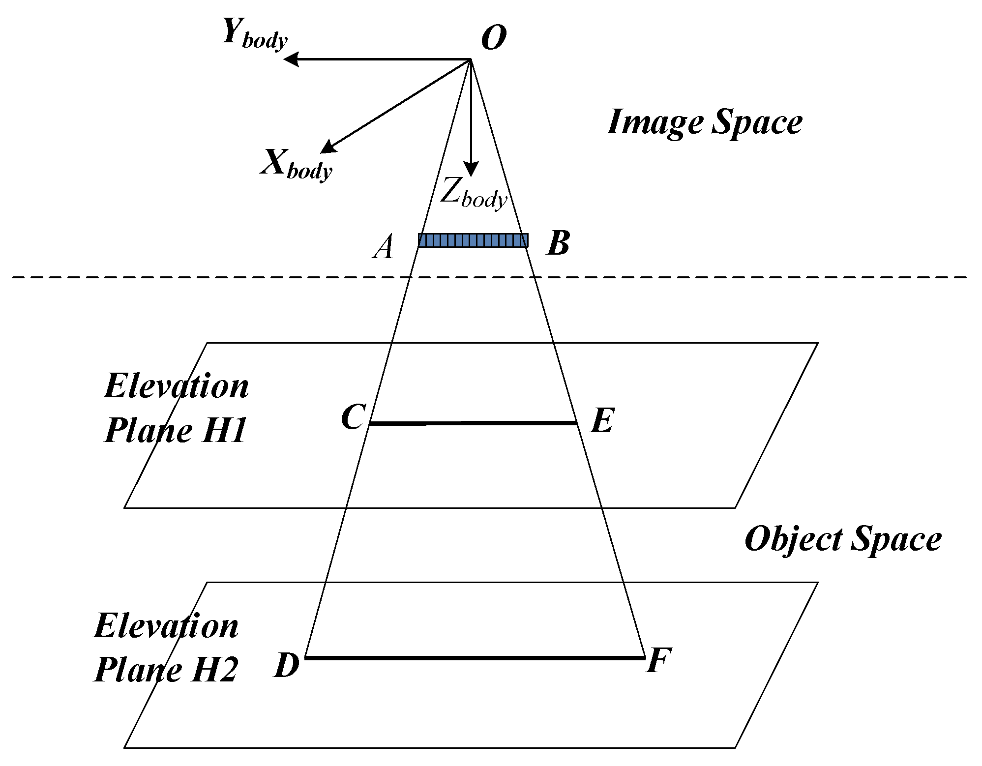
Recovering the RSM from the RFM is to obtain interior and exterior elements. The basic principle of recovering RSM from RFM is shown in Figure 1. In the figure, AB denotes the linear charge-coupled device (CCD) sensor at a certain time; O denotes the position of the projection center, which is an unknown parameter; OA and OB are the rays at linear sensor ends. XYZ stands for the satellite body-fixed coordinate system. H1 and H2 are two elevation planes whose elevations in the geodetic coordinate system are H1 and H2, respectively. The elevation plane H1 intersects ray OA at point C and OB at point D; elevation plane H2 intersects ray OA at point E and OB at point F.
Taking the detector A of the sensor AB at a specified time as an example, the ray OA intersects the elevation planes H1 and H2 at C and E in the object space, respectively. The geographical coordinates of C and E are and respectively. As the detector A is a common feature for ground points C and E, the image coordinates are both . and can be calculated by Equation (3). Then, the coordinates of C and E are and in geocentric Cartesian coordinate system, which can be derived from Equation (4). After the coordinates of C and E are determined, the direction of the ray in the Earth’s geocentric Cartesian coordinate system is the difference between the positions of C and E. This is the basic principle for using the RFM to recover the RSM. First, the position can be solved by the intersection of the vectors EC and FD. Based on the calculation result of the position, the attitude then can be calculated. Considering the correlation between the attitude and the interior orientation elements, the equivalent satellite body-fixed coordinate system is introduced, and its axis points to the ground direction which is the unit vectors of the rays OA and OB. The direction of the axis towards the flight, i.e., perpendicular to the plane OAB. The axis is determined by the axis and axis according to the right-hand criteria. When the axes of the three equivalent ontology coordinate systems are determined in the Earth’s geocentric coordinate system, can then be constructed. Finally, the direction of any ray in the satellite body-fixed coordinate system can be obtained through further applying the rotation matrix .
2.2. Geometric Calibration Model
The calibration model for the linear sensor model was established based on previous work [2,33,34], and it is expressed in Equation (5):
where represent the satellite position, is the rotation matrix, represent the ray direction, m is the unknown scaling factor, represent the unknown ground position, is the offset matrix that compensates for the exterior errors, and denotes the interior orientation elements.
2.2.1. Exterior Calibration Model
can be expanded to Equation (6):
where , , and are rotation angles about the , , and axes in the satellite body-fixed fixed coordinate system, respectively. The measurement errors of attitude and orbit are considered as constant errors within one standard scene, but a degree of random deviation occurs between several scenes imaged at different times, i.e., there are different values for different images.
2.2.2. Interior Calibration Model
Considering that the optical lens distortion is the main cause of error in the interior orientation elements, it is possible to compensate for the interior orientation element error by establishing a lens distortion model. The optical lens distortion error is the deviation of the image coordinates from the ideal coordinates caused by the lens design, fabrication, and assembly. It mainly includes the principal point error , principal distance error , radial distortion error , and decentering distortion error . Assuming that the principal point offset is and the principal distance is , the lens distortion model can be described as follows:
Let , and then the distortion model can be described as follows:
where . For the linear array sensor, where the image coordinate along the track is a constant value, and thus, is set as , the above distortion model can be simplified as follows:
Equation (9) is the distortion model for the compensation of the interior orientation elements. The solving of the compensation model parameters is performed by solving the unknown numbers , , , , , , , and to achieve the compensation for the interior orientation elements. While Equation (9) is a relatively complex non-linear model, there must be an initial value assignment and iterative convergence problems and the stability of the solution will be relatively poor. In order to simplify the solution, Equation (9) can be expanded as follows:
and the following variable substitutions are performed:
Then Equation (10) can be simplified as follows:
Therefore, the above distortion model can be expressed as a quintic polynomial model of the image column variables. The polynomial model is as follows:
where variables and are parameters describing the distortion to be calculated, s is the image coordinate across the track, and l is the image coordinate along the track. It should be noted that the polynomial distortion model can be considered as a one-variable function related to the sample for the linear push-broom camera. Besides, and are not related because the along-track and across-track aberrations in the across-track direction are described independently.
2.3. Solution for Calibration Parameters
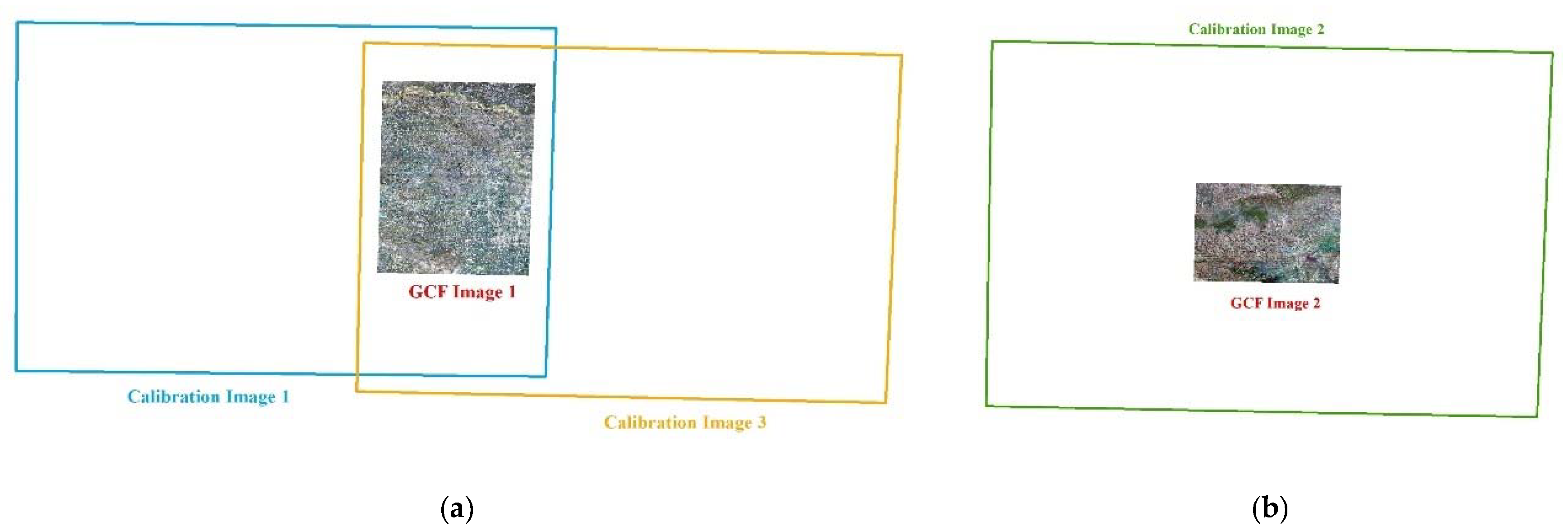
Calibration parameters can be calculated by high-precision GCPs obtained from the geometric calibration field (GCF) image by a high-accuracy matching method. However, on some occasions such as when processing images from a wide-field view camera, it is difficult to obtain sufficient GCPs for the reason that current GCFs fail to cover all rows in only one calibration-wide swath image. Therefore, multiple calibration images are collected to obtain sufficient GCPs covering all the rows. Multiple GCFs cover different parts of these calibration images, which extends the coverage of the GCF information accordingly. As shown in Figure 2, with GCF image 1 covering the right half of calibration image 1 and the left half of calibration image 3, and with GCF image 2 covering the middle part of calibration image 2, all rows in the calibration image can be further covered by the GCF image.
Because multiple calibration images are acquired at different times, there are different exterior orientation elements but the same interior orientation elements for these images. Therefore, it is essential to apply exterior calibration for multiple calibration images before solving the interior orientation element errors. However, owing to the strong correlation between exterior and interior calibration parameters, the compensation residuals of exterior calibration parameters of different images inevitably affect the rightness of interior calibration parameters, i.e., there exists residuals after the compensation of the exterior orientation element errors.
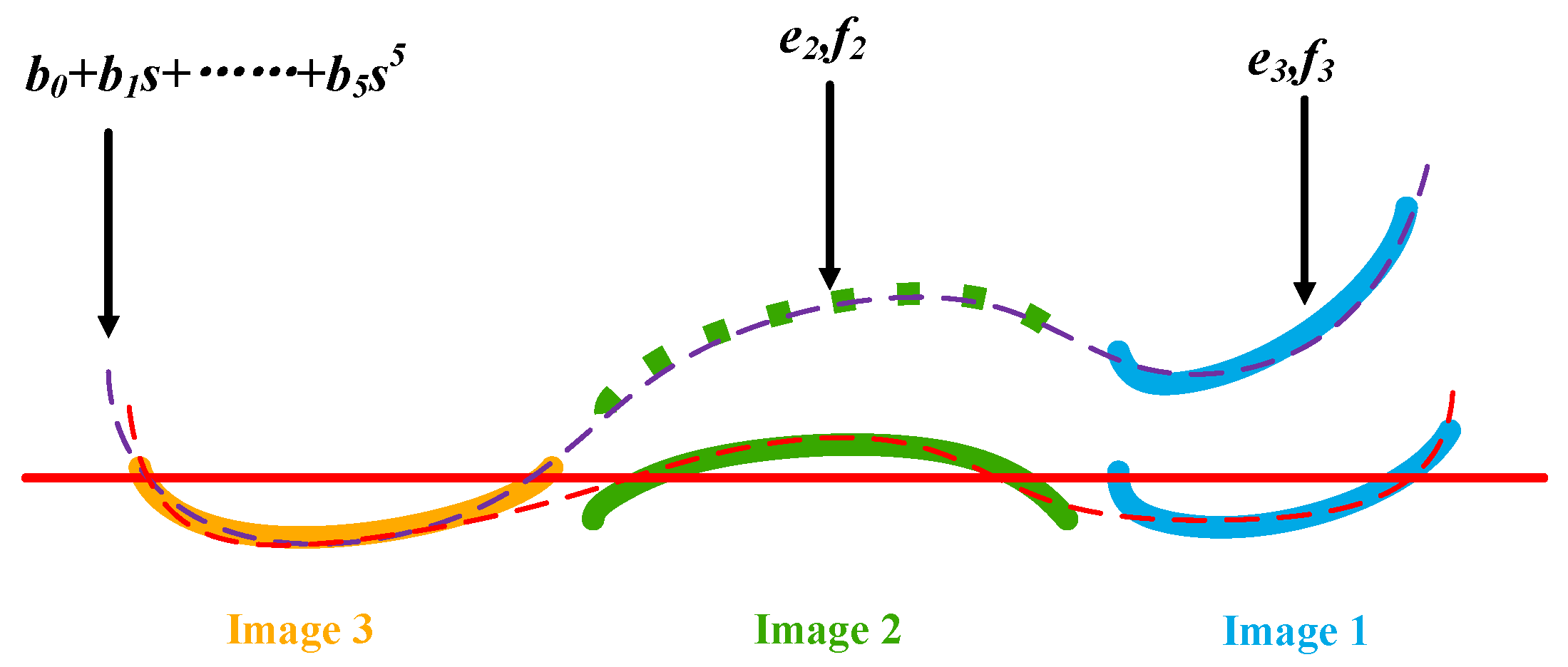
As shown in Figure 3, after three calibration images being compensated by the exterior calibration parameters, taking the across-track error of the calibration image as an example, the residual curve is shown by the solid curve in the diagram (orange, green, blue). The red solid line in the figure is the baseline with an error of zero. It can be seen from the figure that the residual curves of the three calibration images are not continuous (as shown by the red dotted line in the figure) after the compensation of the exterior element errors. Therefore, the interior orientation element errors in the calibration image plane are difficult to fit by Equation (13).
According to [23], when the attitude angle is small, the offset in the image plane caused by the exterior orientation element errors can be described by the shift, shift and scale, affine, and polynomial models. Since the calibration images have been compensated by the exterior calibration parameters, the exterior orientation element errors are much smaller than the previous ones and the residual exterior error can be described by the above model. When considering the orbit error, roll angle error, pitch angle error, and yaw angle error, the orientation error can be described as follows:
where and represent the orientation error caused by the residual exterior error, S represents the orbit error, represents the offset caused by the pitch angle error, represents the yaw angle error, s represents the sample index of a pixel, and the footnotes l and s represent the along-track and across-track values, respectively.
Therefore, in accordance with Equation (14), additional parameters (e, f) are introduced into the polynomial model across the track, which are used to describe the residuals of shift and rotation in the interior orientation elements compensation model. Normally, a calibration image is not introduced, such as calibration image 3 in Figure 3, for computational stability. When these additional parameters are introduced and involved in the adjustment calculations, the other calibration image can be shifted and rotated, and then consequently the resulting residual curve can become continuous (as shown by the red dotted line in Figure 3). The above computational solution process can be seen as an indirect adjustment with a constraint condition, where b0, b1, b2, b3, b4, b5 are the parameters to be requested, and ej and fj are the additional parameters that make the results more reasonable. This is also applicable for the residuals along the track.
Based on the above analysis, the system error compensation model with constrained conditions can be described as follows:
where n denotes the number of calibration images participating in the adjustment calculation, and cj, dj, ej, fj denote additional parameters for each calibration image other than the reference calibration image.
3. Experimental Results
Three experiments were designed to validate our proposed method comprehensively. Experiment 1 was designed to verify the precision of the recovered RSM. Experiment 2 was designed calculate the calibration parameters compensating the systematic error. Experiment 3 was designed to validate the efficiency and rightness of compensation parameters for other non-calibration images, which involves two aspects, namely assessing the orientation accuracy after compensating for exterior errors with four GCPs based on the affine model and testing the elevation accuracy based on block adjustment.
3.1. Study Area and Data Source
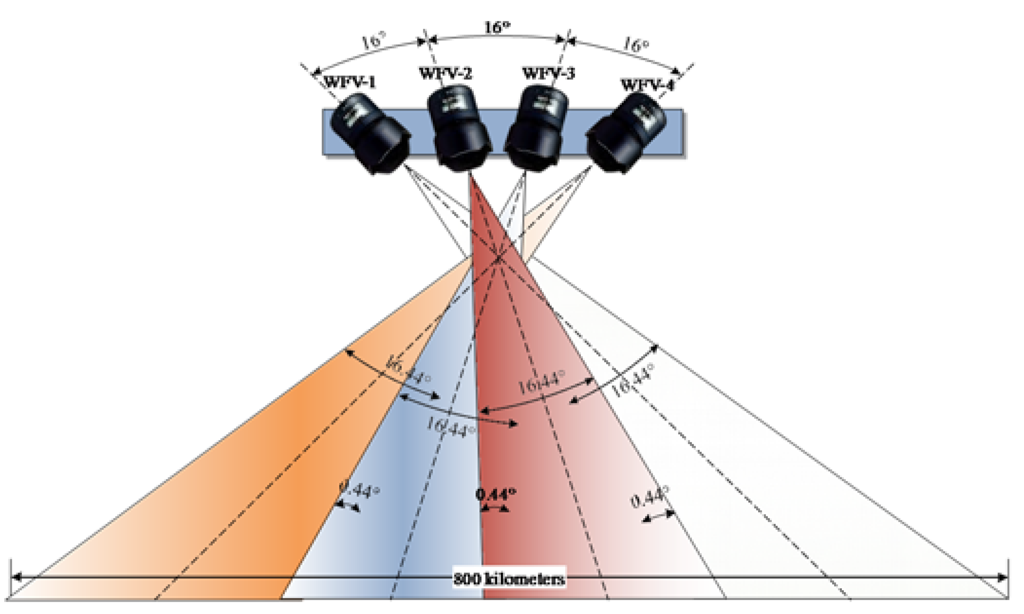
Images captured by the Gaofen-1 (GF-1) wide-field view (WFV) cameras were collected to validate sufficiently the accuracy and reliability of the proposed method. Launched in April 2013 and in a 644.5-km Sun-synchronous orbit, the GF-1 satellite is the first of a series of high-resolution optical Earth observation satellites for CHEOS, and it is mainly used to provide near-real-time observations for disaster prevention and relief, climate change monitoring, and environmental and resource surveys, as well as for precision agriculture support. The GF-1 satellite is configured with a set of four WFV cameras with 16-m multispectral (MS) medium-resolution and a combined swath of 800 km, as shown in Figure 4 [35]. The CCD size of the camera is 0.0065 mm, and the principle distance is about 270 mm. The FOV is about 16.44°, and the image size is 12,000 × 13,400 pixels.
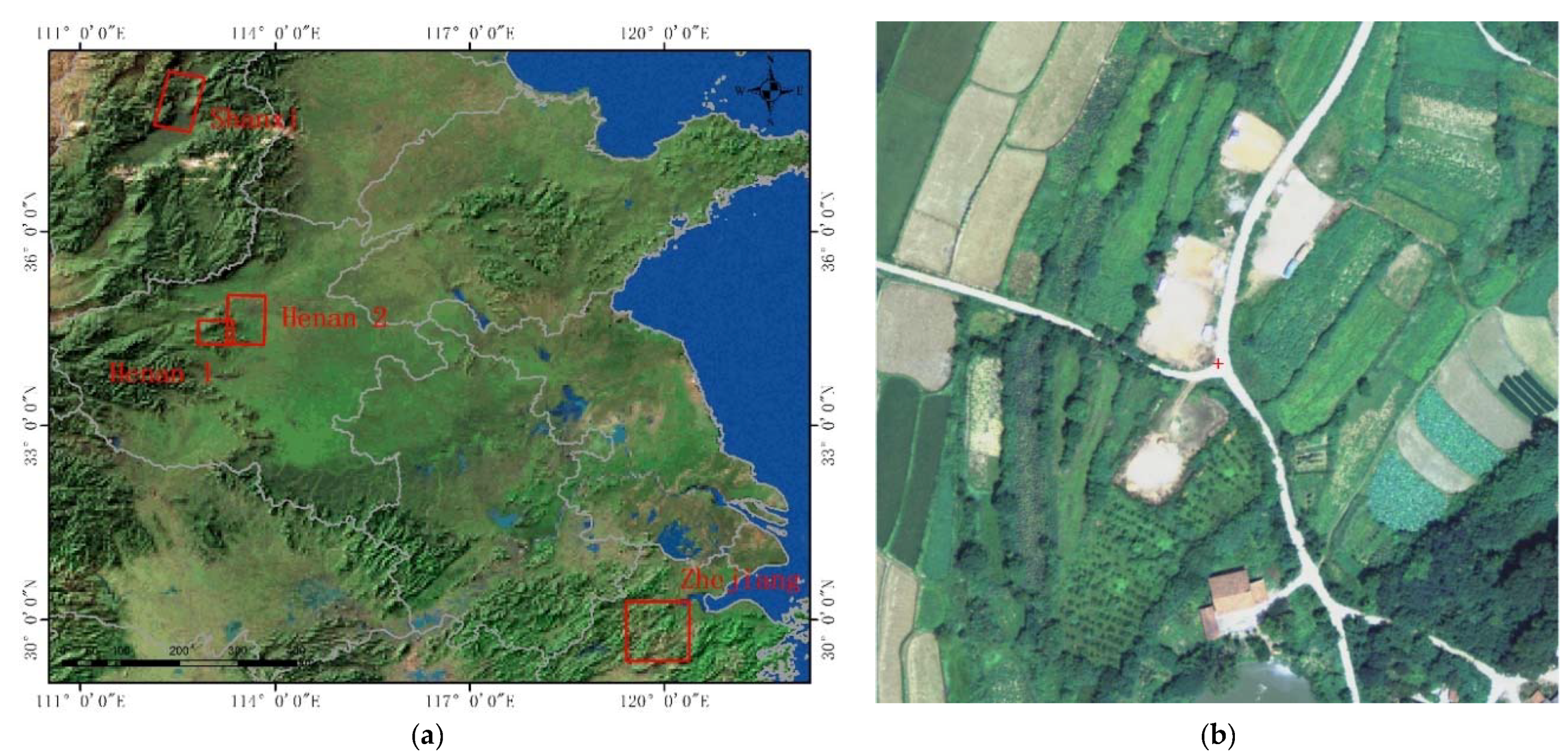
To validate the proposed method, a multitude of experimental GF-1 WFV-1 and WFV-4 images covering the Shanxi, Henan, and Zhejiang areas in China were collected. Detailed information about these images is listed in Table 1 and Table 2, respectively. Among these data, images 2818558, 3000814, 2143625 and 2355539 were collected to calculate the calibration parameters for the WFV-1 camera and images 2453997, 2788768, 2205552 and 2412890 were collected to calculate the calibration parameters for the WFV-4 camera. The GCPs were acquired by the method introduced above that uses the GCF, and the sample range represents the GCF coverage at the start and end rows of the images across the track. Moreover, other images were used to validate the compensation accuracy and elevation accuracy and to conduct digital surface model (DSM) product testing.
The 1:5000 digital orthophoto map/digital elevation model (DOM/DEM) of Henan 1, 1:2000 DOM/DEM of Henan 2, 1:5000 DOM/DEM of Shanxi and 1:10,000 DOM/DEM of Zhejiang as well as 1:5000 averagely distributed GCPs obtained via photographs taken in aerial photography field work in the Zhejiang area, are also applied as reference data. Specific information about GCFs is given in Table 3. Figure 5 presents the spatial coverage of the GCFs and illustration of a GCP.
3.2. Precision of Recovering RSM from RFM
In order to verify the accuracy of recovering the RSM from the RFM, the corresponding RSM was built first by using the interior and exterior orientation elements recovered from the RFM, and then comparisons were made with the RFM. The specific comparison process was as follows: (1) checkpoints were taken at a distance of 1000-pixel intervals on the image space and projected to the average elevation plane to calculate the ground point coordinates by using the RSM; (2) these ground points were conversely projected to the image space by using the RFM; (3) the differences between the two groups of image coordinates (the original and projected image pixel coordinates) were obtained and statistics were compiled to assess the accuracy. As shown in Table 4, the accuracy of the recovered RSM was better than 0.05 pixels for the calibration images. Therefore, for the GF-1 WFV camera, the accuracy loss caused by the recovery of the RSM is negligible.
3.3. Calibration Accuracy Result
Based on the interior and exterior orientation elements recovered from the RFM, geometric calibration was applied for the WFV-1 images and WFV-4 images by the proposed method. To demonstrate the validity of the calibration parameters, the parameters were used to correct the calibration images, and the orientation accuracy with GCPs was determined.
The orientation accuracy obtained by using GCPs before and after the calibration is shown in Table 5 for the WFV-1 images. It can be seen that the orientation accuracy with GCPs was within 0.8 pixels for both the original images and the images after calibration. Generally, the results after calibration were slightly higher than those before calibration. This demonstrates the correctness and effectiveness of the above system error compensation parameters to a certain degree, especially in terms of compensating for distortion errors and achieving improvements in the internal accuracy. The orientation accuracy with GCPs before and after the calibration is shown in Table 6 for the WFV-4 images. The orientation accuracy with GCPs was, within 1 pixel, similar to the other results.
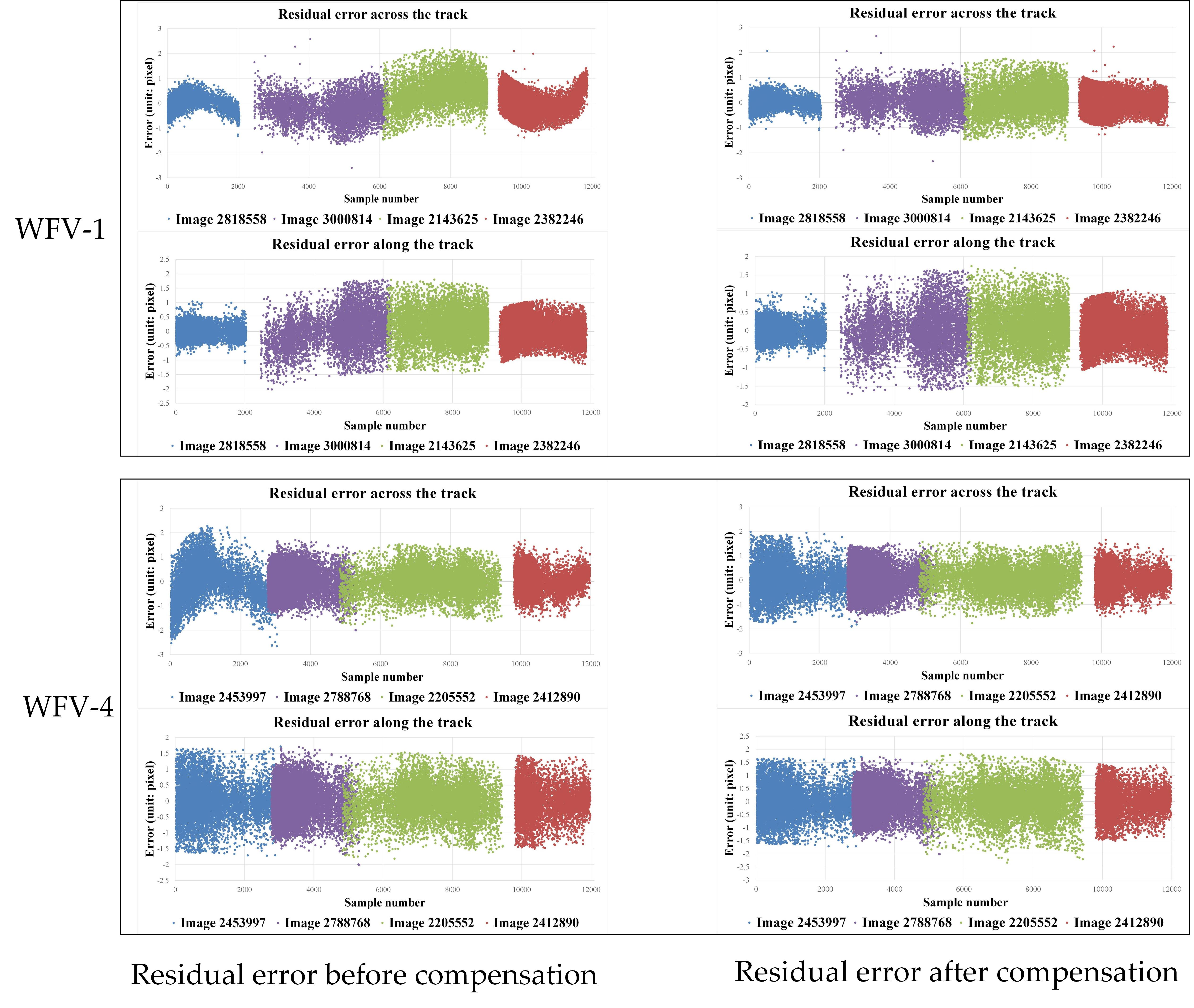
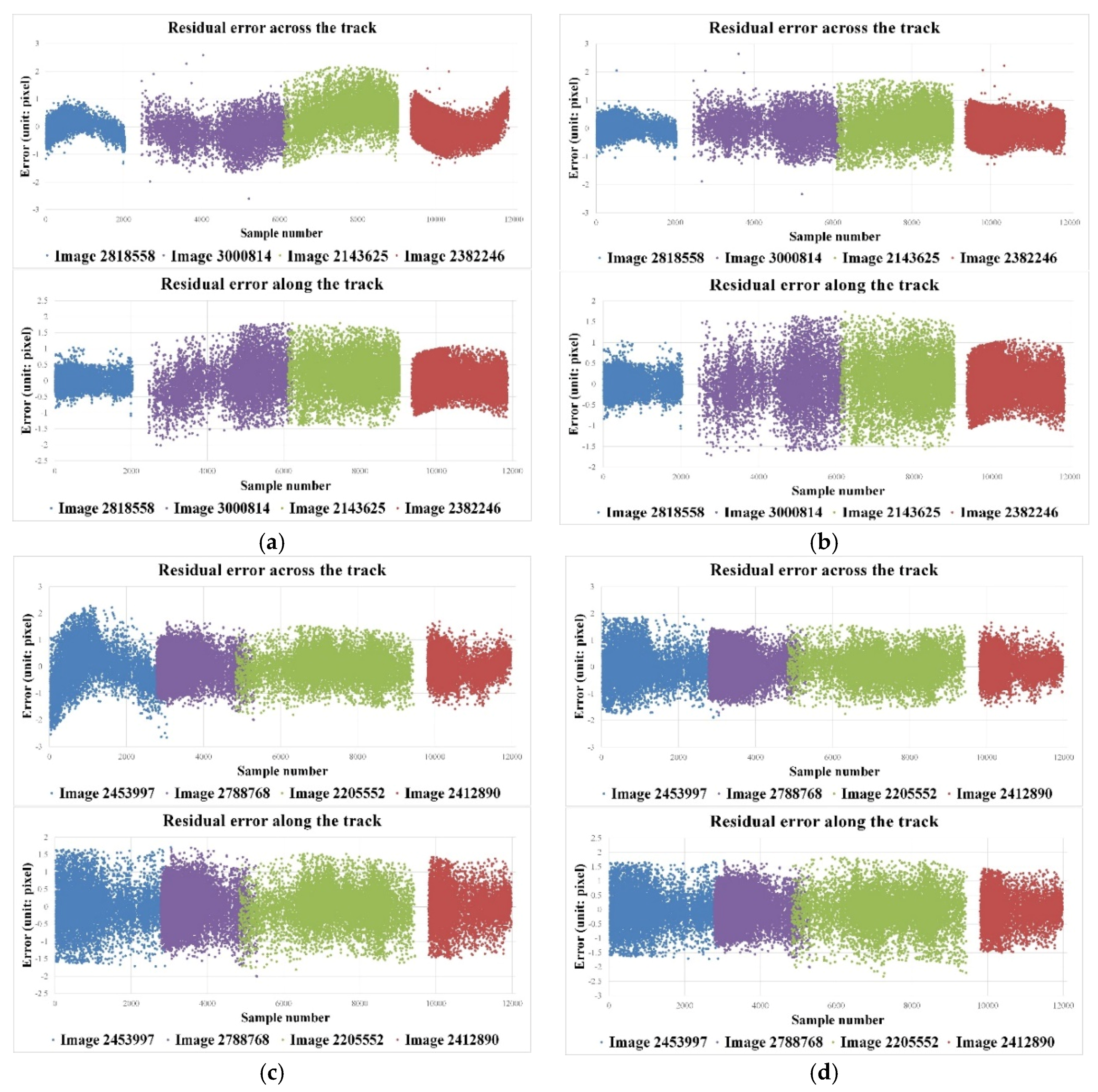
Given that the sample range only covers a part of the image and the exterior orientation absorbed the high-order system errors locally, the effect of error compensation was not obvious, as shown in Table 5 and Table 6. To show the compensation results clearly, Figure 6 presents the residuals before and after the calibration for the WFV-1 and WFV-4 calibration images. The abscissa in the figure indicates the sample number of the image, and the ordinate indicates the residuals. The upper part of the figure represents the residuals across the track, and the lower part represents the residuals along the track. Different colors indicate different calibration scenes.
It can be seen from Figure 6a,c that although the orientation accuracy before compensation was better than 1 pixel, there was significant systematic error before compensation, especially on both ends of the image. This was because the optimization of the orientation process was based on the smallest residual error. Although the residual error value after orientation was small, the internal system error was not fundamentally solved. These systematic errors will severely constrain the use of the data for mapping and, therefore, need to be modeled for elimination according to Equation (15). Figure 6b,d show the residual error after applying the calibration parameters for the WFV-1 and WFV-4 calibration images. Because scenes 108244, 126740, 061400 and 120856 were located at the edges of the images with relatively large distortion errors, it was clear that the results after calibration were much improved in comparison to the results before calibration. Inversely, other images were located at the center of the images with relatively smaller distortion errors, and these results after calibration were close to those before calibration. As seen from the residual plot, residual errors were random and were constrained within 1 pixel, which means that all distortions were corrected and the calibration parameters acquired by the proposed method were effective and correct.
3.4. Compensation Accuracy Result
3.4.1. Validation of Orientation Accuracy
To further validate the proposed method, the calibration parameters were applied to the compensation of other non-calibration images. As shown in Table 7 and Table 8, the orientation accuracies obtained by using GCPs before and after the calibration were within 1 pixel for the WFV-1 and WFV-4 cameras. The results after compensation were slightly higher than those before calibration.
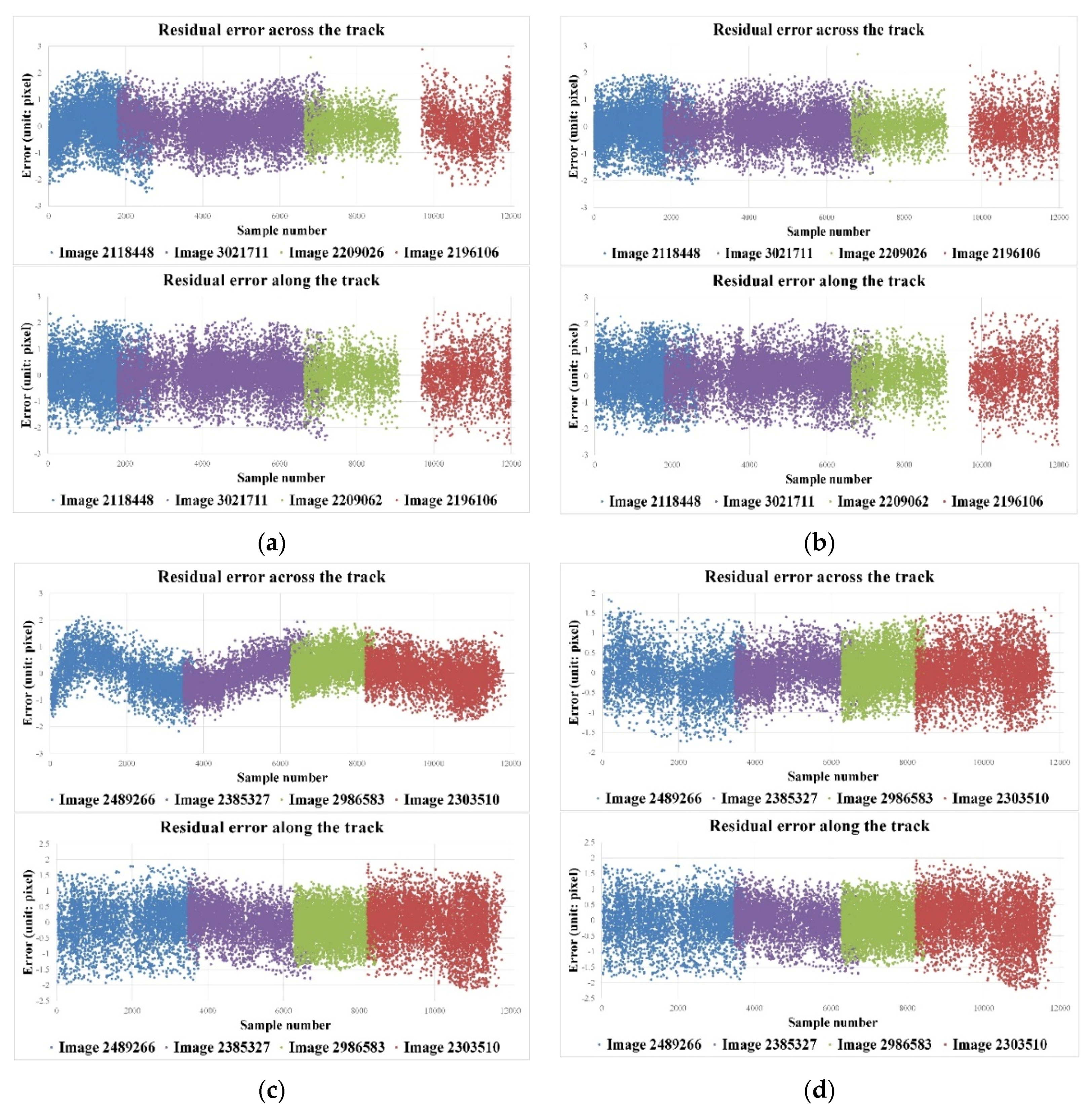
Similarly, considering that the exterior orientation absorbed some interior errors locally and that the sample range only covered a part of the image, it was difficult to observe any residual distortion from Table 4. To observe residual distortion, residual errors before and after the compensation were plotted in Figure 7. It can be seen from Figure 7a,c that although the orientation accuracy before compensation was better than 1 pixel, there was significant systematic error before the compensation, especially at both ends of the image. After applying the calibration parameter compensation, residual errors were random and were constrained within 1 pixel, especially at the ends of the image. There being no obvious systematic errors, this proves that the proposed method is effective and correct for compensation scenes.
Because of the coverage restriction of the GCF, validation using check points (CPs) of GCF cannot reflect the inner accuracy of the entire scene. Thus, GCPs/CPs obtained via photographs taken in aerial photography field work were used to validate the effectiveness of the calibration parameters. As shown in Table 9, the root-mean-square error (RMSE) reached up to 1.1 pixels for image 2143625 and 1.0 pixels for image 2986583. After calibration, the maximum error reached up to 0.9 pixels for scene image 2143625 and 1.0 pixels for scene image 2986583. The RMSE reached up to 0.5 pixels for scene 068316 and 0.6 pixels for scene 112159.
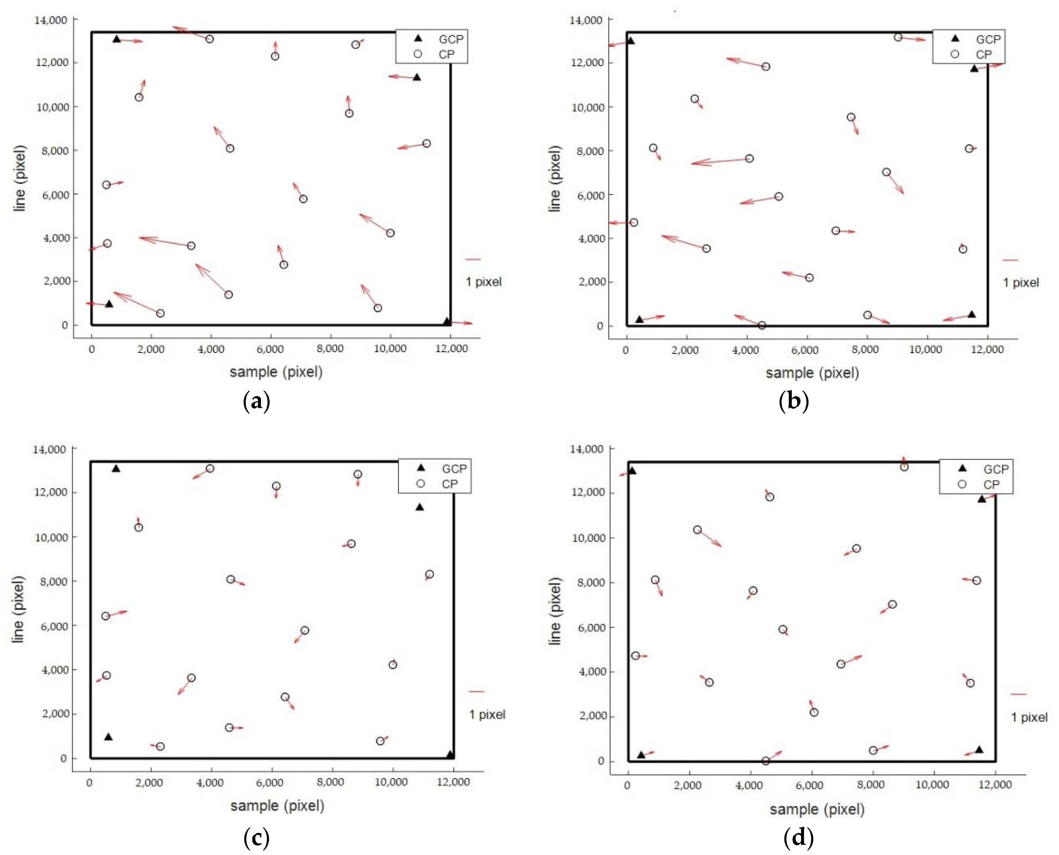
In addition, the orientation residual plots before and after the calibration of images 2143625 and 2986583 are shown in Figure 8. Before applying the compensation, as shown in Figure 8a,c, it can be seen from the plots that the data in the four corners were more accurate than those in other regions, which was because the affine model with four GCPs cannot completely absorb the higher-order distortion effect, especially in the middle region. After calibration, as shown in Figure 8b,d, it can be seen that the accuracy level was consistently within 0.6 pixels and the residual errors were random. In short, the non-linear system error was eliminated after applying the compensation, and the images represented undistorted images whose residual system error could be absorbed by the affine model with four GCPs. Thus, the orientation accuracy was improved after the compensation, and the results after orientation can be used for further applications.
3.4.2. Validation of Elevation Accuracy
As shown in Figure 4, the WFV cameras can observe the same area only if in different orbits, thus providing the potential for surveying and mapping. To obtain better intersection accuracy, the WFV-1 and WFV-4 cameras were taken as an example to analyze the height accuracy. According to [36,37], the ratio between the elevation accuracy and plane accuracy is as follows:
where and represent the horizontal error and vertical error, respectively. is the length of the baseline, and is the flight height. Thus, the vertical error can be calculated by the following equation:
Considering that the orbit height of GF-1 is 644.5 km, the baseline between WFV-1 and WFV-4 is about 600 km. According to Section 3.4.1, the orientation accuracy for the WFV image is approximately 0.5 pixels, and the corresponding point extraction accuracy is about 0.3 pixels too. The resolution of the WFV-1 or WFV-4 images is about 16 m. Theoretically, the horizontal vertical accuracy for the GF-1 are 12.8 m and 11.9 m, respectively, according to Equation (18):
According to the stereo analysis, the elevation accuracy for the GF-1 WFV-1 and WFV-4 cameras will be about 11.9 m. As the above calibration accuracy and matching accuracy are approximate, the stereo accuracy is a reference value that will be variant for each pixel.
In order to validate the stereo accuracy of the images before and after applying the compensation, stereo pairs formed from the overlapping area of WFV-1 image 2143265 and WFV-4 image 2886583 were processed with block adjustments by using different numbers of GCPs. The block adjustment results are given in Table 10 and, as shown, whether without GCPs or with GCPs, the stereo accuracies after applying the compensation with calibration parameters exhibited superior performance in comparison to the original ones. It is the geometric distortion in the image that results in the poor geometric quality for the original image. While for the images after compensation the plane accuracy with four GCPs can reach 8 m, and the elevation accuracy can reach about 11 m, which has reached the accuracy limit for the WFV images with a 16-m resolution, this can fulfill requirements for 1:100,000 stereo mapping in mountainous areas.
4. Discussion
4.1. Imporatance of Separating System Errors during Compensation
Since the initial missions and goals for GF-1 were land and resources surveys, the image distortion was not considered excessively in camera design, or an improper in-orbit geometric calibration was carried compared with a cartographic satellite, and then system errors still disappeared. As shown in Figure 6a,c and Figure 8a,c, there exist obvious non-linear system errors and the orientation accuracy with GCPs is poor. As analyzed in Section 2.2, the errors induced by exterior orientation elements errors exhibit linear form, while the errors induced by interior elements errors exhibit high-order non-linear form. Therefore, the real influence of geometric performance for a non-cartographic satellite’s image is the interior orientation errors. These errors would deteriorate the geometric quality of the image and further affect subsequent applications, especially in cartographic use. Moreover, previous studies demonstrated that the relationship between the quality of the DSM and the interior distortion of camera. From the references [38,39], uncalibrated IKONOS images will result in a bias of about 0.3–1.7 m in the DSM, which are mainly attributed to the interior distortion. Consequently, eliminating such non-linear systematic errors caused by interior orientation errors is a crucial precondition for enabling the non-cartographic satellite’s images with the capability of mapping and improving the application benefits.
During the compensation, it is essential to discriminate system errors from its features. The proposed method considers the stability of system errors to overcome the problem of traditional system error compensation in fitting residuals from the result. The static errors mainly contain optical lens distortion, i.e., interior orientation errors, and non-static errors stand for exterior orientation errors. Since this strategy directly starts from the causes of systematic errors, various approximate assumptions and conditional constraints of many traditional strategies can be avoided, overcoming the stringent conditions that conventional strategies require a narrow camera field and small attitude errors, and extending the method of compensating the system errors of a basic remote-sensing image.
As shown in Table 5, Table 6, Table 7 and Table 8, a comparison of orientation accuracy before and after applying compensation parameters was made. Although the improvement effect numerically was not obvious, there were clear high-order non-linear system errors induced by lens distortion shown in the corresponding residual figures, especially at both ends of images. Figure 4 also explains that the wide field angle (16.44°) creates large lens distortion in the image.
Due to the limitation of the cover range of the GCF images and the wide swath of the WFV camera (up to 200 km), the control points obtained by the GCF of each image can only cover a portion of its width. In the local area of the image, the systematic error of the whole image, especially the distortion error, cannot be reflected originally. The high-order distortion curve for the whole scene performed a low-order curve in the local scope. Most of the low-order residuals were absorbed by the exterior orientation model used in the orientation process, resulting in relatively high accuracy without compensation. Therefore, the aforementioned comparison of the accuracy of before and after compensation does not completely reflect the situation of the whole image. To further show the improvement effect of the compensation, we manually selected 20 GCPs evenly distributed in the whole image to examine the orientation accuracy. All the subfigures in Figure 8 demonstrate that the orientation accuracy was increasingly improved and the residual errors were random after the compensation.
4.2. Calculateing Calibration Paramters using Multi-Geometric Calibration Field (GCF) for Wide-Field View (WFV) Camera
It is difficult to obtain sufficient GCPs from current GCFs built in China, because current GCFs fail to cover all rows in only one image due to the wide swath of GF-1 WFV. As shown in Figure 4, the swath of the GF-1 WFV image spans 200 km. The proposed solution of calibration parameters by multi-GCFs can provide a usable approach for calculating calibration parameters to overcome the difficulty of the swath of the image becoming wider than current available GCFs. It is noted that the multiple calibration images should be captured within a shorter interval to guarantee them sharing same internal distortion. In addition, considering that the eccentric distortion of the aerospace camera is very small, the error along the track manifests shift error and the errors across the track is fifth-order according to Equation (13). This also explains why the interior distortion of the linear push-broom camera is mainly in the across-track direction.
4.3. Compensation Parameters Availability
Conventional error-compensation models mainly are to fit or approximate the residuals from the results and to perform corrections on the RFM based on additional parameters. Starting with the causes of system errors, the proposed method recovers the RSM model firstly then compensates the errors based on dividing the errors into static errors and non-static errors for each image. Consequently, the compensation parameters can be applied to other images rather than only be efficient within one image like the traditional BCM. In Section 3.4, the experimental results validate the rightness and efficiency of compensation parameters for other validation images.
The availability of compensation parameters is mainly subject to whether the non-linear distortions change in the acquisition time of validation images. In a previous study of geometric calibration of ZY3-02 satellite, we validated the stability of internal accuracy, concluding that the variations in imaging time (within two months) and area have less of an influence on the internal accuracy, with the maximum discrepancy being equal to 0.06 pixels [34]. In addition, other researchers demonstrated that the interior calibration parameters are relatively stable in the short term and tried to establish the changing trend models within four years [40]. Moreover, according to the satellite designer from China Academy of Space Technology, they adopted some technologies like thermal control to provide a comparable environment for cameras on board satellites. The imaging date of experimental images in this paper span approximately 1 year, and the estimated interior calibration parameters are relatively stable within short periods.
However, with the aging of devices and the change of external environment, the state of the camera (interior calibration parameters) would vary and compensation parameters become invalid. It is important to monitor the change of distortion to avoid bad affects from the change of system errors. We advise that the non-linear system errors should be monitored frequently and compensation parameters updated in a timely fashion.
4.4. Accuracy Loss Analysis
In the process of system error compensation, there exist links of precision loss: recovering the RSM from corresponding RFM, acquisition of GCPs, the system error compensation model and its solution, and generating the new improved RFM with compensation parameters. GCPs acquisition and systematic error compensation models and their solutions are difficult to evaluate, but the recovery of RSM and the generation of RFM can be evaluated based on the pros and cons of the model before and after recovery (generation). Taking into account the general requirement of the orientation accuracy with GCPs is required to be within 1 pixel, hence 1 pixel will be used as a benchmark to evaluate the recovery accuracy of the RSM and the generation accuracy of the RFM.
The recovery accuracy of the RSM is valued by comparing the difference of the image coordinate between the forward calculation using the recovered RSM and the inverse calculation using the original RFM. Table 4 shows the accuracy loss of recovering RSM from the RFM. It can be seen that the accuracy of the RSM is within 0.05 pixels. Therefore, for the GF-1 WFV-1 and WFV-4 camera, the accuracy loss caused by the recovery of the RSM is negligible. Similarly, the generation accuracy of the new RFM is valued by generating statistics on the difference of the image coordinate between the forward calculation using compensated RSM and the inverse calculation using compensated RFM. As can be seen from Table 11, the RFM generation accuracy for all calibration images is approximately 0.1 pixels, except that images 2382246 and 2453997 reach 0.2 pixels. In general, the accuracy loss of generating RFM satisfies the requirement.
5. Conclusions
In this paper, a novel method was proposed to improve the geometric performance for a non-cartographic satellite’s imagery. Unlike conventional BCM methods, this method compensates for the system errors based on their cause rather than by simply building a compensation model according to the fit or to approximate the residuals. The proposed method recovers the RSM from the RFM first, and then it compensates for the system errors of the non-cartographic satellite’s images by using the conventional geometric calibration method based on the RSM; finally, a new and improved RFM is generated. Images captured by the WFV-1 camera and WFV-4 camera onboard GF-1 were collected as experimental data. Several conclusions can be drawn from the analysis, and these can be summarized.
There exist obvious non-linear system errors across the track for GF-1 WFV images before applying the compensation, which adversely affect the potential for using the data in surveying and mapping applications and thus reduce the application effectiveness of Earth observation data. After employing this proposed method, images exhibited superior orientation accuracy compared to the original ones. Experiments demonstrated that the orientation accuracy of the proposed method evaluated by CPs was within 1 pixel for both the calibration images and validation images, and the residual errors manifested in a random distribution. Validation by using the CPs obtained via photographs taken in aerial photography field work further proved the effectiveness of the proposed method, and the entire scene was undistorted compared to that without applying the calibration parameters. Moreover, for the validation of the elevation accuracy, block adjustment tests showed that the vertical accuracy had improved from 21 m to 11 m with four GCPs, and these values were coincident with the theoretical values. Generally, these findings demonstrate the potential of using a non-cartographic optical remote-sensing satellite’s images for mapping by the proposed method.
Author Contributions
G.Z., Q.Z. and D.L. conceived and designed the experiments; K.X., G.Z. and M.D. performed the experiments; M.D. analyzed the data; K.X. and M.D. wrote the paper.
Acknowledgments
This work was supported by the Key research and development program of Ministry of science and technology (2016YFB0500801), the National Natural Science Foundation of China (Grant No. 91538106, Grant No. 41501503, 41601490, Grant No. 41501383), the China Postdoctoral Science Foundation (Grant No. 2015M582276), the Hubei Provincial Natural Science Foundation of China (Grant No. 2015CFB330), the Special Fund for High-Resolution Images Surveying and Mapping Application System (Grant No. AH1601-10), and the Quality improvement of domestic satellite data and comprehensive demonstration of geological and mineral resources (Grant No. DD20160067). The authors also thank the anonymous reviewers for their constructive comments and suggestions.
Conflicts of Interest
The authors declare no conflict of interest.
References
- Pan, H.B.; Zhang, G.; Tang, X.M.; Li, D.R.; Zhu, X.Y.; Zhou, P.; Jiang, Y.H. Basic products of the ziyuan-3 satellite and accuracy evaluation. Photogramm. Eng. Remote Sens. 2013, 79, 1131–1145. [Google Scholar] [CrossRef]
- Jiang, Y.H.; Zhang, G.; Tang, X.M.; Li, D.R.; Huang, W.C.; Pan, H.B. Geometric calibration and accuracy assessment of ziyuan-3 multispectral images. IEEE Trans. Geosci. Remote Sens. 2014, 52, 4161–4172. [Google Scholar] [CrossRef]
- Gu, X.F.; Tong, X.D. Overview of China earth observation satellite programs [space agencies]. IEEE Geosci. Remote Sens. Mag. 2015, 3, 113–129. [Google Scholar]
- Li, D.R.; Shen, X.; Ma, H.C.; Zhang, G. Commercial operation of China’s high-resolution earth observation system is imperative. Geomat. Inf. Sci. Wuhan Univ. 2014, 39, 386–389. [Google Scholar]
- Tuyahov, A.J. The earth observing system for the 1990 and 2000 decades. Sci. Total Environ. 1986, 56, 3–15. [Google Scholar] [CrossRef]
- Stackhouse, P.; Wald, L.; Renne, D.; Meyer, R. Towards designing an integrated earth observation system for the provision of solar energy resource and assessment. In Proceedings of the IEEE International Conference on Geoscience and Remote Sensing Symposium, Denver, CO, USA, 31 July–4 August 2006; pp. 3517–3520. [Google Scholar]
- Neeck, S.P.; Magner, T.J.; Paules, G.E. NASA’S small satellite missions for earth observation. Acta Astronaut. 2005, 56, 187–192. [Google Scholar] [CrossRef]
- Sapritsky, V.I.; Krutikov, V.N.; Ivanov, V.S.; Panfilov, A.S.; Pavlovich, M.N.; Burdakin, A.A.; Rakov, V.V.; Morozova, S.P.; Lisyansky, B.E.; Khlevnoy, B.B. Current activity of Russia in measurement assurance of earth optical observations. Metrologia 2012, 49, 633–635. [Google Scholar] [CrossRef]
- Shimada, M.; Tadono, T.; Rosenqvist, A. Advanced land observing satellite (ALOS) and monitoring global environmental change. Proc. IEEE 2010, 98, 780–799. [Google Scholar] [CrossRef]
- Mcguire, M.E.; Parashar, S.; Mahmood, A.; Brule, L. Evolution of Canadian earth observation from radarsat-1 to radarsat-2. In Proceedings of the IEEE 2001 International Geoscience and Remote Sensing Symposium, Sydney, NSW, Australia, 9–13 July 2001; Volume 481, pp. 480–481. [Google Scholar]
- Radhadevi, P.V.; Solanki, S.S. In-flight geometric calibration of different cameras of IRS-P6 using a physical sensor model. Photogramm. Rec. 2008, 23, 69–89. [Google Scholar] [CrossRef]
- Dial, G.; Bowen, H.; Gerlach, F.; Grodecki, J.; Oleszczuk, R. Ikonos satellite, imagery, and products. Remote Sens. Environ. 2003, 88, 23–36. [Google Scholar] [CrossRef]
- Ager, T.P. Evaluation of the geometric accuracy of ikonos imagery. Proc. SPIE 2003, 5093, 613–620. [Google Scholar]
- Fraser, C.S.; Ravanbakhsh, M. Georeferencing accuracy of geoeye-1 imagery. Photogramm. Eng. Remote Sens. 2009, 75, 634–638. [Google Scholar]
- Noguchi, M.; Fraser, C.S.; Nakamura, T.; Shimono, T.; Oki, S. Accuracy assessment of quickbird stereo imagery. Photogramm. Rec. 2004, 19, 128–137. [Google Scholar] [CrossRef]
- Poli, D.; Wolff, K.; Gruen, A. Evaluation of worldview-1 stereo scenes and related 3d products. Remote Sens. Spat. Inf. Sci. 2009, 38, 1–4. [Google Scholar]
- Pu, R.L.; Landry, S. A comparative analysis of high spatial resolution ikonos and worldview-2 imagery for mapping urban tree species. Remote Sens. Environ. 2012, 124, 516–533. [Google Scholar] [CrossRef]
- Chevrel, M.; Courtois, M.; Weill, G. The spot satellite remote sensing mission. Photogramm. Eng. Remote Sens. 1981, 47, 1163–1171. [Google Scholar]
- Topan, H.; Cam, A.; Özendi, M.; Oruç, M.; Jacobsen, K.; Taşkanat, T. Pl iades project: Assessment of georeferencing accuracy, image quality, pansharpening performence and DSM/DTM quality. Int. Arch. Photogramm. Remote Sens. 2016, 41, 503–510. [Google Scholar] [CrossRef]
- Agency, X.N. China to Launch Jilin-1 Satellite in October. Available online: http://www.chinadaily.com.cn/china/2015-08/04/content_21499539.htm (accessed on 4 August 2015).
- Fraser, C.S.; Hanley, H.B. Bias compensation in rational functions for ikonos satellite imagery. Photogramm. Eng. Remote Sens. 2003, 69, 53–58. [Google Scholar] [CrossRef]
- Aguilar, M.A.; Saldaña, M.D.M.; Aguilar, F.J. Assessing geometric accuracy of the orthorectification process from geoeye-1 and worldview-2 panchromatic images. Int. J. Appl. Earth Obs. Geoinf. 2013, 21, 427–435. [Google Scholar] [CrossRef]
- Grodecki, J.; Dial, G. Block adjustment of high-resolution satellite images described by rational polynomials. Photogramm. Eng. Remote Sens. 2003, 69, 59–70. [Google Scholar] [CrossRef]
- Tong, X.H.; Liu, S.J. Rational polynomial coefficients generation and physical sensor model recovery for high resolution satellite stereo imagery. Sci. Online 2008, 11, 003. [Google Scholar]
- Teo, T.A. Line-based rational function model for high-resolution satellite imagery. Int. J. Remote Sens. 2013, 34, 1355–1372. [Google Scholar] [CrossRef]
- Takaku, J.; Tadono, T. RPC generations on ALOS prism and AVNIR-2. In Proceedings of the 2011 Geoscience and Remote Sensing Symposium, Vancouver, BC, Canada, 24–29 July 2011; pp. 539–542. [Google Scholar]
- Liu, J.H.; Jia, B.; Jiang, T.; Jiang, G.W. Extrapolative positioning of RPC model of Th-1 satellite Three-Line imagery. Geomat. Spat. Inf. Technol. 2013, 9, 20–21. [Google Scholar]
- Jiang, Y.H.; Zhang, G.; Chen, P.; Li, D.R.; Tang, X.M.; Huang, W.C. Systematic error compensation based on a rational function model for ziyuan1-02c. IEEE Trans. Geosci. Remote Sens. 2015, 53, 3985–3995. [Google Scholar] [CrossRef]
- Cao, J.S.; MA, L.H. Systematic error compensation for object positioning of zy-3 images. Sci. Surv. Mapp. 2015, 40, 3–8. [Google Scholar]
- Xiong, Z.; Zhang, Y. A generic method for RPC refinement using ground control information. Photogramm. Eng. Remote Sens. 2009, 75, 1083–1092. [Google Scholar] [CrossRef]
- Hu, Y.; Tao, C.V. Updating solutions of the rational function model using additional control information. Photogramm. Eng. Remote Sens. 2002, 68, 715–724. [Google Scholar]
- Tao, C.V.; Hu, Y. A comprehensive study of the rational function model for photogrammetric processing. Photogramm. Eng. Remote Sens. 2001, 67, 1347–1357. [Google Scholar]
- Tang, X.M.; Zhang, G.; Zhu, X.Y.; Pan, H.B.; Jiang, Y.H.; Zhou, P.; Wang, X. Triple linear-array image geometry model of ziyuan-3 surveying satellite and its validation. Int. J. Image Data Fusion 2012, 4, 33–51. [Google Scholar] [CrossRef]
- Xu, K.; Jiang, Y.H.; Zhang, G.; Zhang, Q.J.; Wang, X. Geometric potential assessment for ZY3-02 triple linear array imagery. Remote Sens. 2017, 9, 658. [Google Scholar] [CrossRef]
- Bai, Z.G. Gf-1 satellite—The first satellite of Cheos. Aerosp. China 2013, 14, 11–16. [Google Scholar]
- Zhang, Y.J. Analysis of precision of relative orientation and forward intersection with high-overlap images. Geomat. Inf. Sci. Wuhan Univ. 2005, 30, 126–130. [Google Scholar]
- Zhang, Y.J.; Lu, Y.H.; Wang, L.; Huang, X. A new approach on optimization of the rational function model of high-resolution satellite imagery. IEEE Trans. Geosci. Remote Sens. 2012, 50, 2758–2764. [Google Scholar] [CrossRef]
- Baltsavias, E.P. DSM generation and interior orientation determination of IKONOS images using a testfield in Switzerland. In Proceedings of the ISPRS Hannover Workshop 2005 on “High-Resolution Earth Imaging for Geospatial Information”, Hannover, Germany, 17–20 May 2006; pp. 41–54. [Google Scholar]
- Zhang, L.; Gruen, A. Multi-image matching for DSM generation from ikonos imagery. ISPRS J. Photogramm. Remote Sens. 2006, 60, 195–211. [Google Scholar] [CrossRef]
- Takaku, J.; Tadono, T. Prism on-orbit geometric calibration and DSM performance. IEEE Trans. Geosci. Remote Sens. 2009, 47, 4060–4073. [Google Scholar] [CrossRef]
Figure 1.
Schematic diagram of the principle of recovering the rigorous sensor model (RSM) from the rational function model (RFM).
Figure 1.
Schematic diagram of the principle of recovering the rigorous sensor model (RSM) from the rational function model (RFM).

Figure 2.
Schematic diagram of ground control points (GCPs) acquisition strategy for wide swath image. (a) Geometric calibration field (GCF) image 1 covers the right half of calibration image 1 and the left half of calibration image 3; (b) GCF image 2 covering the middle part of calibration image 2.

Figure 3.
Schematic diagram of the system error compensation model with constrained conditions.

Figure 4.
Schematic diagram of wide-field view (WFV) camera onboard GF-1 satellite.

Figure 5.
(a) Spatial coverage of the images of GCF; (b) image showing a corresponding 1:5000 GCP obtained via photographs taken in aerial photography field work.
Figure 5.
(a) Spatial coverage of the images of GCF; (b) image showing a corresponding 1:5000 GCP obtained via photographs taken in aerial photography field work.

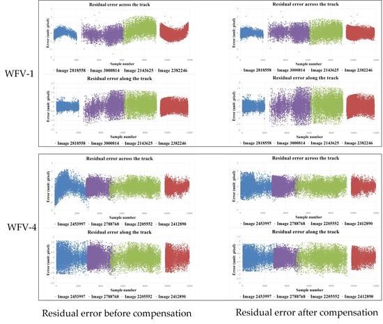
Figure 6.
Residual error before and after calibration. The horizontal axis denotes the image row across the track and the vertical axis denotes residual errors after orientation. (a) WFV-1 residual error before calibration; (b) WFV-1 residual error after calibration; (c) WFV-4 residual error before calibration; (d) WFV-4 residual error after calibration.

Figure 7.
Residual error before and after compensation. The horizontal axis denotes the image row across the track and the vertical axis denotes residual errors after orientation. (a) WFV-1 residual error before compensation; (b) WFV-1 residual error after compensation; (c) WFV-4 residual error before compensation; (d) WFV-4 residual error after compensation.

Figure 8.
Orientation errors before and after applying compensation parameters. (a) Image 2143625 before compensation; (b) image 2143625 after compensation; (c) image 2986583 before compensation; (d) image 2986583 after compensation.
Figure 8.
Orientation errors before and after applying compensation parameters. (a) Image 2143625 before compensation; (b) image 2143625 after compensation; (c) image 2986583 before compensation; (d) image 2986583 after compensation.


Table 1.
Detailed information for the experimental images of Gf-1 WFV-1 camera.
| Image ID | Camera | Area | Acquisition Data | Function | Sample Range (Pixel) |
|---|---|---|---|---|---|
| 2818558 | WFV-1 | Shanxi | 3 December 2017 | Calibration | 10–2000 |
| 3000814 | WFV-1 | Zhejiang | 13 February 2018 | Calibration | 2460–6220 |
| 2143625 | WFV-1 | Zhejiang | 24 January 2017 | Calibration | 6100–9040 |
| 2355539 | WFV-1 | Shanxi | 12 May 2017 | Calibration | 9350–11,880 |
| 2118448 | WFV-1 | Henan | 3 January 2017 | Validation | 10–2690 |
| 3021711 | WFV-1 | Henan | 23 February 2018 | Validation | 1800–7230 |
| 2209026 | WFV-1 | Henan | 27 February 2017 | Validation | 6640–9130 |
| 2196106 | WFV-1 | Henan | 19 February 2017 | Validation | 9670–11,980 |
Table 2.
Detailed information for experimental images of Gf-1 WFV-4 camera.
| Image ID | Camera | Area | Acquisition Data | Function | Sample Range (Pixel) |
|---|---|---|---|---|---|
| 2453997 | WFV-4 | Shanxi | 1 July 2017 | Calibration | 20–3050 |
| 2788768 | WFV-4 | Shanxi | 22 November 2017 | Calibration | 2770–5360 |
| 2205552 | WFV-4 | Henan | 24 February 2017 | Calibration | 4820–9450 |
| 2412890 | WFV-4 | Shanxi | 7 June 2017 | Calibration | 9800–11,980 |
| 2489266 | WFV-4 | Zhejiang | 16 July 2017 | Validation | 20–3750 |
| 2385327 | WFV-4 | Zhejiang | 28 May 2017 | Validation | 3470–6810 |
| 2986583 | WFV-4 | Zhejiang | 6 February 2018 | Validation | 6270–8520 |
| 2303510 | WFV-4 | Zhejiang | 13 April 2017 | Validation | 8210–11,860 |
Table 3.
Specific information about the GCF image.
| Area | GSD of DOM (m) | Plane Accuracy of DOM RMS (m) | Height Accuracy of DEM RMS (m) | Range (km2) (across Track × along Track) | Center Latitude and Longitude |
|---|---|---|---|---|---|
| Shanxi | 0.5 | 1 | 1.5 | 50 × 95 | 38.00°N, 112.52°E |
| Henan 1 | 0.5 | 1 | 1.5 | 50 × 41 | 34.65°N, 113.55°E |
| Henan 2 | 0.2 | 0.4 | 0.7 | 54 × 84 | 34.45°N, 113.07°E |
| Zhejiang | 1 | 2 | 3 | 90 × 90 | 29.87°N, 119.88°E |
Table 4.
Precision of recovering RSM from RFM for calibration images (unit: pixel).
| Image ID | Residual between RSM and RFM | ||
|---|---|---|---|
| Max | Min | RMS | |
| 2818558 | 0.132 | 0.000 | 0.027 |
| 3000814 | 0.135 | 0.000 | 0.028 |
| 2143625 | 0.127 | 0.000 | 0.047 |
| 2382246 | 0.120 | 0.000 | 0.045 |
| 2453997 | 0.107 | 0.000 | 0.038 |
| 2788768 | 0.113 | 0.000 | 0.041 |
| 2205552 | 0.093 | 0.000 | 0.035 |
| 2412890 | 0.192 | 0.000 | 0.046 |
Table 5.
Orientation accuracy before and after calibration evaluated by GCF CPs (Check points) for WFV-1 camera images (unit: pixel).
Table 5.
Orientation accuracy before and after calibration evaluated by GCF CPs (Check points) for WFV-1 camera images (unit: pixel).
| Image ID | No. GCPs/CPs | Line | Sample | Max | Min | RMS | |
|---|---|---|---|---|---|---|---|
| 2818558 | 4/9705 | Ori. | 0.223 | 0.300 | 1.327 | 0.000 | 0.374 |
| Cal. | 0.222 | 0.243 | 2.055 | 0.000 | 0.329 | ||
| 3000814 | 4/7082 | Ori. | 0.601 | 0.491 | 2.605 | 0.000 | 0.776 |
| Cal. | 0.362 | 0.474 | 2.649 | 0.000 | 0.596 | ||
| 2143625 | 4/8874 | Ori. | 0.536 | 0.556 | 2.204 | 0.000 | 0.772 |
| Cal. | 0.536 | 0.525 | 1.752 | 0.000 | 0.750 | ||
| 2382246 | 4/18,782 | Ori. | 0.353 | 0.388 | 2.100 | 0.000 | 0.525 |
| Cal. | 0.570 | 0.319 | 2.227 | 0.000 | 0.653 |
Ori.: original, Cal.: calibration.
Table 6.
Orientation accuracy before and after calibration evaluated by GCF CPs for WFV-4 camera images (unit: pixel).
Table 6.
Orientation accuracy before and after calibration evaluated by GCF CPs for WFV-4 camera images (unit: pixel).
| Image ID | No.GCPs/Cps | Line | Sample | Max | Min | RMS | |
|---|---|---|---|---|---|---|---|
| 2453997 | 4/8863 | Ori. | 0.573 | 0.757 | 2.659 | 0.000 | 0.949 |
| Cal. | 0.572 | 0.613 | 1.979 | 0.000 | 0.838 | ||
| 2788768 | 4/14,738 | Ori. | 0.478 | 0.478 | 2.004 | 0.000 | 0.676 |
| Cal. | 0.478 | 0.515 | 1.722 | 0.000 | 0.703 | ||
| 2205552 | 4/10,953 | Ori. | 0.484 | 0.484 | 1.810 | 0.000 | 0.684 |
| Cal. | 0.575 | 0.480 | 1.765 | 0.000 | 0.749 | ||
| 2412890 | 4/6264 | Ori. | 0.531 | 0.468 | 1.682 | 0.000 | 0.708 |
| Cal. | 0.531 | 0.454 | 1.653 | 0.000 | 0.699 |
Ori.: original, Cal.: calibration.
Table 7.
Orientation accuracy before and after compensation for WFV-1 camera images (unit: pixel).
| Image ID | No. GCPs/CPs | Line | Sample | Max | Min | RMS | |
|---|---|---|---|---|---|---|---|
| 2111848 | 4/6382 | Ori. | 0.721 | 0.700 | 2.465 | 0.000 | 1.005 |
| Com. | 0.720 | 0.665 | 2.119 | 0.000 | 0.980 | ||
| 3021711 | 4/10,238 | Ori. | 0.817 | 0.584 | 2.073 | 0.000 | 1.004 |
| Com. | 0.816 | 0.561 | 1.960 | 0.000 | 0.990 | ||
| 2209026 | 4/2310 | Ori. | 0.616 | 0.497 | 2.585 | 0.000 | 0.791 |
| Com. | 0.616 | 0.495 | 2.689 | 0.000 | 0.790 | ||
| 2196106 | 4/2100 | Ori. | 0.648 | 0.762 | 2.882 | 0.000 | 1.000 |
| Com. | 0.643 | 0.669 | 2.269 | 0.000 | 0.928 |
Ori.: original, Com.: compensation.
Table 8.
Orientation accuracy before and after compensation for WFV-4 camera images (unit: pixel).
| Image ID | No. GCPs/Cps | Line | Sample | Max | Min | RMS | |
|---|---|---|---|---|---|---|---|
| 2489266 | 4/4556 | Ori. | 0.652 | 0.694 | 2.172 | 0.000 | 0.952 |
| Com. | 0.645 | 0.538 | 1.838 | 0.000 | 0.840 | ||
| 2385327 | 4/4628 | Ori. | 0.531 | 0.574 | 1.928 | 0.000 | 0.782 |
| Com. | 0.517 | 0.393 | 1.403 | 0.000 | 0.649 | ||
| 2986583 | 4/5776 | Ori. | 0.496 | 0.472 | 1.863 | 0.000 | 0.685 |
| Com. | 0.494 | 0.451 | 1.418 | 0.000 | 0.669 | ||
| 2303510 | 4/5893 | Ori. | 0.689 | 0.562 | 1.776 | 0.000 | 0.889 |
| Com. | 0.700 | 0.538 | 1.639 | 0.000 | 0.883 |
Ori.: original, Com.: compensation.
Table 9.
Orientation accuracy with four ground control points (GCPs) (unit: pixel).
| Image ID | No. of GCPs/CPs | Line | Sample | Max | Min | RMS | |
|---|---|---|---|---|---|---|---|
| 2143625 | 4/16 | Ori. | 0.701 | 0.859 | 1.855 | 0.567 | 1.110 |
| Com. | 0.320 | 0.353 | 0.867 | 0.045 | 0.476 | ||
| 2986583 | 4/16 | Ori. | 0.414 | 0.926 | 1.954 | 0.237 | 1.015 |
| Com. | 0.384 | 0.40 | 1.056 | 0.285 | 0.559 |
Ori.: original, Com.: compensation.
Table 10.
Block adjustment results of before and after applying compensation parameters for stereo images of 2143265 (WFV-1) and 2986583 (WFV-4) in Zhejiang area.
Table 10.
Block adjustment results of before and after applying compensation parameters for stereo images of 2143265 (WFV-1) and 2986583 (WFV-4) in Zhejiang area.
| No. of GCPs/CPs | Root-Mean-Square Error (RMSE) of GCPs (m) | RMSE of CPs (m) | |||||||
|---|---|---|---|---|---|---|---|---|---|
| North | East | Plane | Height | North | East | Plane | Height | ||
| 0/15 | Ori. | - | - | - | - | 27.621 | 38.546 | 47.421 | 33.010 |
| Com. | - | - | - | - | 24.001 | 44.030 | 50.147 | 29.821 | |
| 1 in center/14 | Ori. | 0 | 0 | 0 | 0 | 15.140 | 20.604 | 25.568 | 38.545 |
| Com. | 0 | 0 | 0 | 0 | 13.329 | 23.802 | 27.280 | 19.858 | |
| 4 in corners/11 | Ori. | 1.330 | 4.126 | 4.336 | 4.923 | 6.072 | 8.077 | 10.105 | 21.483 |
| Com. | 1.609 | 4.649 | 4.920 | 6.285 | 4.348 | 6.386 | 7.726 | 10.859 | |
| 15/0 | Ori. | 4.330 | 7.070 | 8.291 | 17.677 | - | - | - | - |
| Com. | 3.550 | 5.817 | 6.815 | 9.905 | - | - | - | - | |
Ori.: original, Com.: compensation.
Table 11.
Precision of generating RFM (unit: pixel).
| Image ID | Max | Min | RMS |
|---|---|---|---|
| 2818558 | 0.329 | 0.000 | 0.121 |
| 3000814 | 0.336 | 0.000 | 0.125 |
| 2143625 | 0.284 | 0.000 | 0.113 |
| 2382246 | 0.499 | 0.000 | 0.207 |
| 2453997 | 0.407 | 0.000 | 0.213 |
| 2788768 | 0.227 | 0.000 | 0.073 |
| 2205552 | 0.241 | 0.000 | 0.078 |
| 2412890 | 0.296 | 0.000 | 0.086 |
© 2018 by the authors. Licensee MDPI, Basel, Switzerland. This article is an open access article distributed under the terms and conditions of the Creative Commons Attribution (CC BY) license (http://creativecommons.org/licenses/by/4.0/).
Share and Cite
MDPI and ACS Style
Xu, K.; Zhang, G.; Deng, M.; Zhang, Q.; Li, D. Improving Geometric Performance for Imagery Captured by Non-Cartographic Optical Satellite: A Case Study of GF-1 WFV Imagery. Remote Sens. 2018, 10, 971. https://doi.org/10.3390/rs10060971
AMA Style
Xu K, Zhang G, Deng M, Zhang Q, Li D. Improving Geometric Performance for Imagery Captured by Non-Cartographic Optical Satellite: A Case Study of GF-1 WFV Imagery. Remote Sensing. 2018; 10(6):971. https://doi.org/10.3390/rs10060971
Chicago/Turabian StyleXu, Kai, Guo Zhang, Mingjun Deng, Qingjun Zhang, and Deren Li. 2018. "Improving Geometric Performance for Imagery Captured by Non-Cartographic Optical Satellite: A Case Study of GF-1 WFV Imagery" Remote Sensing 10, no. 6: 971. https://doi.org/10.3390/rs10060971
Note that from the first issue of 2016, this journal uses article numbers instead of page numbers. See further details here.