Focusing High-Resolution Highly-Squinted Airborne SAR Data with Maneuvers


1
National Lab. of Radar Signal Processing, Xidian University, Xi’an 710071, China
2
Department of Electronic Engineering, City University of Hong Kong, Hong Kong, China
*
Author to whom correspondence should be addressed.
Remote Sens. 2018, 10(6), 862; https://doi.org/10.3390/rs10060862
Submission received: 24 April 2018
/
Revised: 24 May 2018
/
Accepted: 29 May 2018
/
Published: 1 June 2018
(This article belongs to the Special Issue Radar Imaging in Challenging Scenarios from Smart and Flexible Platforms)
Abstract
:Maneuvers provide flexibility for high-resolution highly-squinted (HRHS) airborne synthetic aperture radar (SAR) imaging and also mean complex signal properties in the echoes. In this paper, considering the curved path described by the fifth-order motion parameter model, effects of the third- and higher-order motion parameters on imaging are analyzed. The results indicate that the spatial variations distributed in range, azimuth, and height directions, have great impacts on imaging qualities, and they should be eliminated when designing the focusing approach. In order to deal with this problem, the spatial variations are decomposed into three main parts: range, azimuth, and cross-coupling terms. The cross-coupling variations are corrected by polynomial phase filter, whereas the range and azimuth terms are removed via Stolt mapping. Different from the traditional focusing methods, the cross-coupling variations can be removed greatly by the proposed approach. Implementation considerations are also included. Simulation results prove the effectiveness of the proposed approach.
1. Introduction
In recent years, there have been tremendous studies on synthetic aperture radar (SAR). As an active sensor, SAR is able to work day and night under all weather conditions [1,2,3]. In addition, SAR can operate at different frequencies and view angles in different polarimetric modes. This feature makes the SAR a flexible and effective tool for information retrieval [4,5,6]. With the advancement of SAR, high resolution and highly squint angle have potential to provide more information about the surface structure. Moreover, the SAR platform is capable of flying along a curved path to realize different applications, to the extent that the model assumption of the rectilinear path no longer holds. This scenario occurs in SAR systems on aircraft platforms because of various factors such as rugged topography, atmospheric turbulence, and intended maneuvers [7,8,9,10]. Characteristics of a curved path differ from those of a uniform linear motion. Major peculiarities exist in its motion parameters, non-uniform spatial-intervals, and three-dimensional (3-D) spatial geometric model. Thus, the traditional imaging algorithms based on straight trajectory and hyperbolic range model (HRM) may be invalid. In order to guarantee the imaging qualities, both the range model and the imaging algorithm may need to change. In addition, the maneuvers will greatly affect the spatial variations in both the range and azimuth directions, particularly for the high-resolution highly-squinted (HRHS) SAR.
In the literature, the fourth-order Doppler range model (FORM) [11,12,13], modified equivalent squint range model (MESRM) [14], advanced hyperbolic range equation (AHRE) [15], equivalent range model (ERM) [16], and modified ERM (MERM) [17] for spaceborne or airborne SAR have been proposed to describe the curved path. Compared with the conventional HRM, these models introduce acceleration into the range model, which makes the descriptions of characteristics, including Doppler bandwidth, cross-coupling phase, and two-dimensional (2-D) spatial variations, of the raw-data more accurate. However, they only consider the acceleration term and ignore the higher-order motion parameters, which limit their applications for high-accuracy imaging. In reality, the maneuvers cannot always be controlled only by constant velocity and acceleration, thus the higher-order motion parameters are needed [18]. If this problem cannot be well solved, it may strongly impair the final image quality in terms of geometric distortion and radiometric resolution losses for HRHS SAR [5]. Thus, profound research on the geometrical model is still necessary.
Concerning the focusing algorithm for the SAR with maneuvers, methods performed in the frequency domain include the range-Doppler algorithm (RDA) [19], chirp scaling algorithm (CSA) [20], omega-K algorithm (OKA) [21], and their extensions [11,12,13,22,23,24,25]. Eldhuset [11,12] suggests a fourth-order processing algorithm by 2-D exact transfer function (ETF) for spaceborne SAR with curved orbit. However, this work ignores the 2-D spatial variation of the azimuth modulation phase and results in defocusing in the azimuth edge regions. Luo et al. [13] and Wang et al. [14] respectively propose a modified RDA and a modified CSA, which can greatly remove the cross-coupling terms brought by the curved path. However, the spatial variations of the acceleration have not been considered. Li et al. [23] propose a frequency-domain algorithm (FDA) for the small-aperture highly-squinted airborne SAR with maneuvers. With expanding the azimuth time in a small aperture, the azimuth spatial variation of the stripmap SAR can be eliminated. However, the residual errors increase greatly with the aperture (resolution). Moreover, the neglected range and vertical spatial variations of the azimuth modulation phase cannot be ignored for the HRHS SAR with maneuvers. The wavenumber domain algorithm [17] and OKA [22] for the HRHS SAR with curved path are proposed based on different modified equivalent range models, which can avoid using the method of series reversion (MSR) to achieve the 2-D spectrum. However, the residual spatial variations caused by approximations would lead to deteriorations in the final image. The 2-D keystone transform algorithms (KTAs) are developed in [26] based on the 2-D Taylor series expansion and they can greatly remove the spatial variations of the high-resolution spaceborne SAR. The errors introduced by the 2-D Taylor expansion can be ignored for the spaceborne SAR but not for the HRHS SAR. Generally, the 2-D spatial variations are not eliminated entirely by [11,12,13,14,15,16,17,18,19,20,21,22,23,24] performed in frequency domain and have great impacts on the final image result. Wu et al. [27] propose a hybrid correlation algorithm (HCA) for the curved flight path, which treats the 2-D correlation by a combination of frequency-domain fast correlation in azimuth dimension and time-domain convolution in the range dimension. Furthermore, back projection algorithm (BPA) and fast factorized BPA (FFBPA) [28,29,30,31] have been suggested. However, in terms of computational burden, the HCA and BPA are not always the best choices compared with the frequency-domain algorithms. The polar format algorithm (PFA) [5,32] can be used for the three-dimensional (3-D) acceleration cases. However, the depth of field is seriously affected by the wavefront curvature, and it must be extended by subaperture technique for the quadratic phase error (QPE) compensation. Thus, further studies are still required for the HRHS SAR with maneuvers.
In this paper, the fifth-order motion parameter model is introduced and the problems are discussed for the HRHS SAR with maneuvers, which are the important factors that demand attention in imaging design. Our analyses suggest that the spatial variations in arbitrary direction brought by the third- and higher-order motion parameters cannot be ignored. Employing the Taylor series expansions with multi-variables, we decompose the spatial variations into three parts—i.e., range, azimuth, and cross-coupling terms—with a high accuracy. Then, according to the properties of decomposed phases, the polynomial phase filter and Stolt mapping with interpolations are performed to remove the cross-coupling and range/azimuth spatial variations, respectively. Unlike the traditional focusing algorithms [11,12,13,14,15,23,24], the cross-coupling spatial variations, which are always ignored in low-resolution case, are corrected for the HRHS SAR with maneuvers. Implementation considerations, including simplified processing and constraint on scene extent are also studied.
The rest of this paper is organized as follows. The signal model of HRHS SAR with maneuvers is investigated and the confronting problems are presented in Section 2. In Section 3, our imaging approach is presented. Implementation considerations are provided in Section 4. Numerical simulation results are given to validate the proposed approach in Section 5. Conclusions are drawn in Section 6.
2. Modeling and Motivation
2.1. Modeling
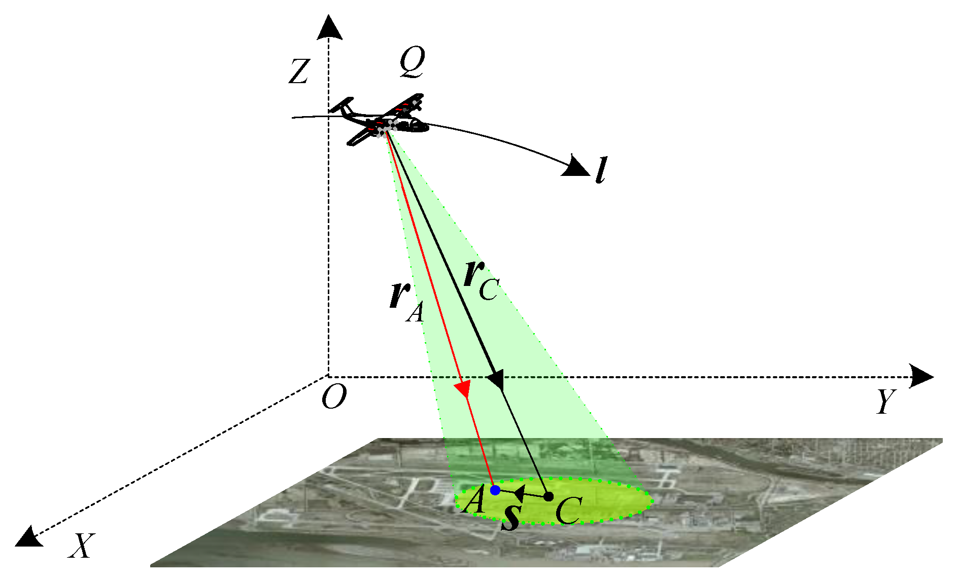
Figure 1 shows the geometric model of the HRHS SAR with maneuvers. The projection of radar location on the ground is assumed to be the origin of Cartesian coordinates O-XYZ. Assuming that points C and A are respectively the central reference point (CRP) and an arbitrary point on the scene, is the flight path of the platform, point Q is the position of the platform at the aperture center moment (ACM), and and are respectively the position vectors of platform to points C and A at ACM.
According to the imaging geometry shown in Figure 1 and the kinematics equation of the platform, the instantaneous slant range history corresponding to arbitrary point A can be expressed as
where is the symbol of absolute value, is the velocity vector, and is the acceleration vector, while , , and are the third-, fourth-, and fifth- order motion parameter vectors in the motion Equation (1), respectively. It is obvious that the range history is an equation with higher-order terms shown as a flat-top shape. It is difficult to derive the 2-D spectrum directly using Equation (1) based on the principle of stationary point (POSP); therefore, the traditional SAR processing methods cannot be applied directly. One way to treat the complex fifth-order motion parameter model (FMPM) is to expand it into a power series in azimuth time as
where the first six coefficients are
In Equation (1), , , and are respectively the slant range, Doppler centroid, and Doppler frequency modulation (FM) of the point A. , , and are the higher-order terms which have great impact on the final image qualities and cannot be ignored.
By using the range history expressed in Equation (1), we obtain the received echo as
where is the range fast time, is the speed of light, and are the carrier frequency and FM rate of the transmitted signal respectively, is the complex scattering coefficient, and and are the range and azimuth windows in time domain.
Based on Equation (2), Equation (9) is transformed into the range frequency domain using the POSP after range compression, i.e.,
where is the range frequency and is the range window in frequency domain.
2.2. Motivation
(1) Error Analysis of FMPM: Traditionally, and are always taken into consideration for the SAR with maneuvers. However, in the case of HRHS SAR, this second-order motion parameter equation is insufficient and it will greatly deteriorate the final image results and limit the scene size. In this work, the higher-order motion parameter vectors, namely, , , and are exploited to improve the accuracy of the flight path description.
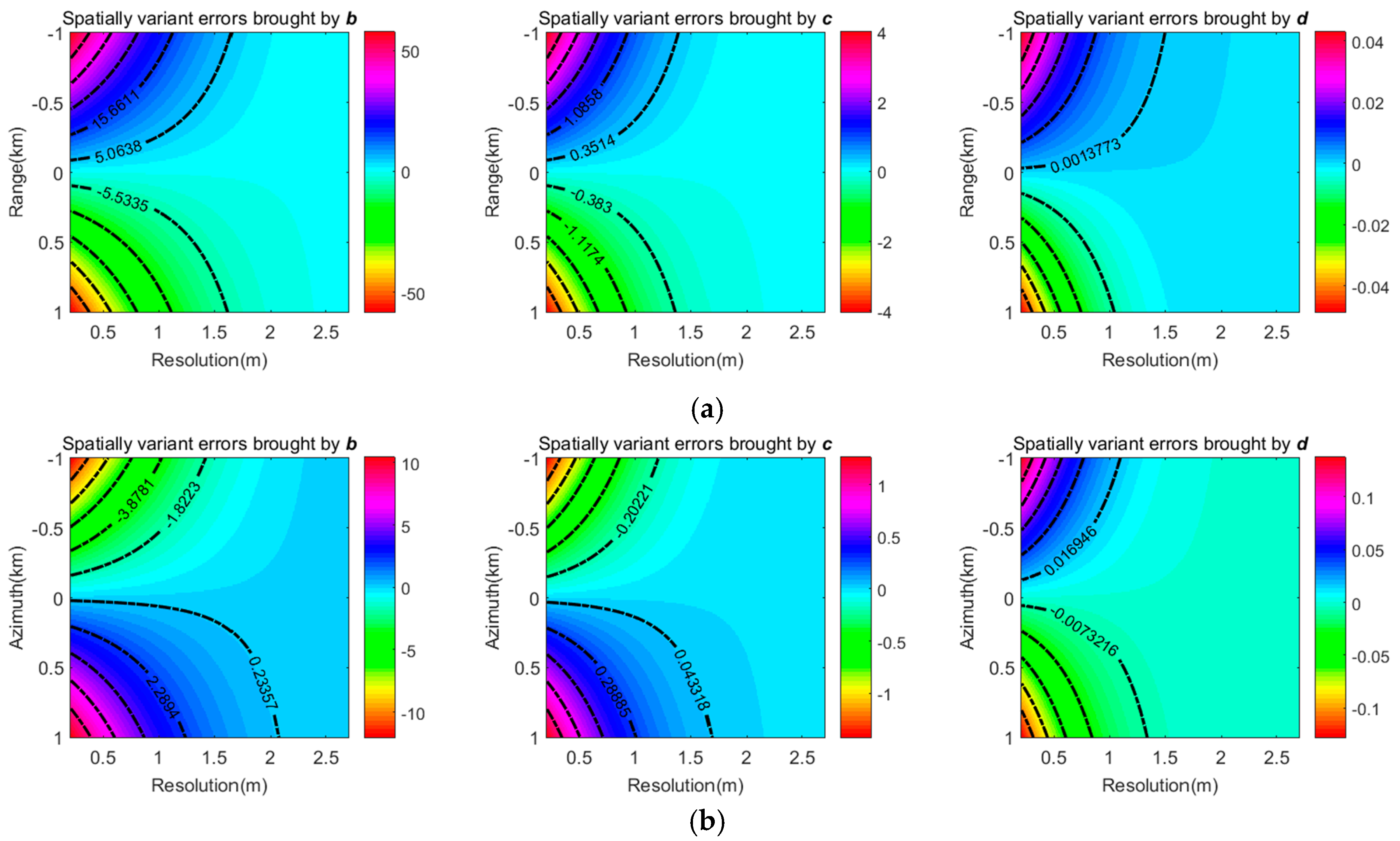
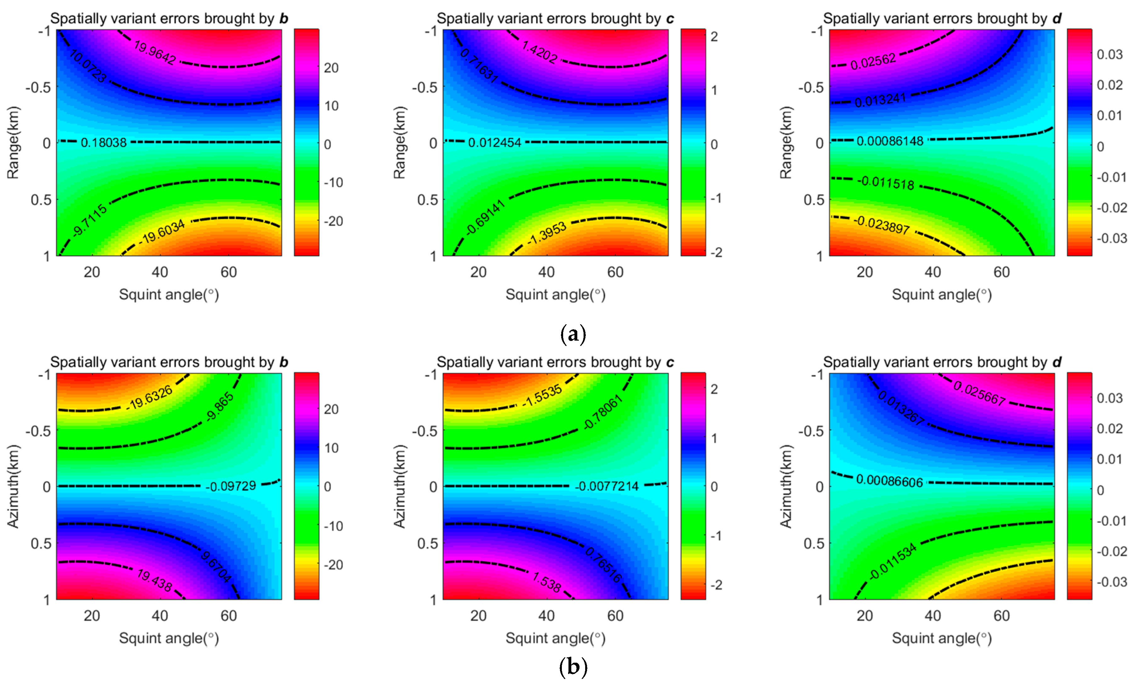
Employing the parameters listed in Table 1, Figure 2a,b respectively show the phase errors and spatially variant errors caused by the motion parameter vectors , , and . The unit of the contour maps is . Note that spatially variant errors brought by can be ignored, whereas both the phase errors by , , and and the spatially variant errors by and cannot. Figure 3a,b respectively show the spatially variant errors with different azimuth resolutions in range and azimuth directions. Clearly, the effects of and must be taken into consideration for the high-resolution cases whereas that of is negligible. Figure 4a,b respectively show the spatially variant errors with different squint angles in range and azimuth directions. The maximum errors at large squint angles are far larger than introduced by and . The impacts brought by are still small enough and can be ignored. According to the above analyses, the spatial variations brought by the motion parameter vectors and should be considered.
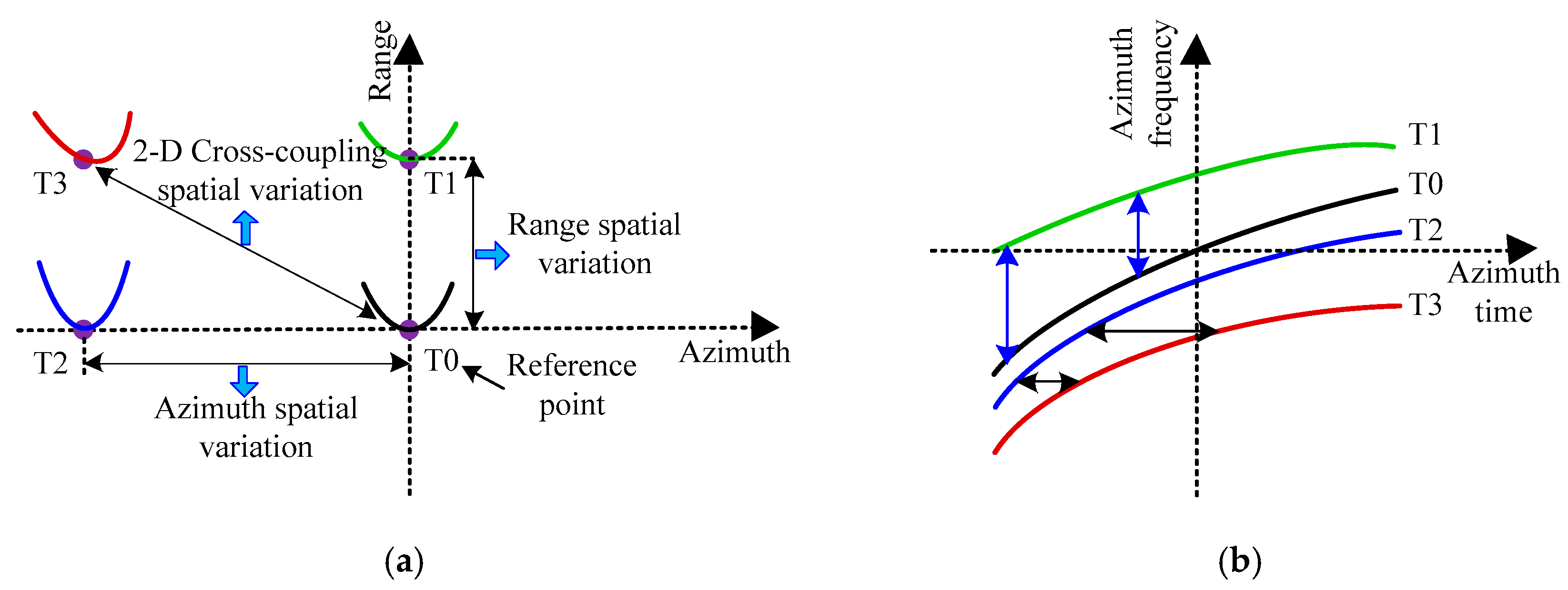
(2) Irregularly Spatial Variation Distributions: As analyzed in the above part, the spatial variation should be taken into consideration for the HRHS SAR with maneuvers to achieve a high quality image and it exists in all the targets, with different range curvatures, with respect to the reference one on the scene. To better understand the existing spatial variations of the targets on the scene, an illustration is provided in Figure 5, where T0 is the reference point, T1 and T2 are the targets that respectively have the same azimuth and range cells as those of T0, and T3 is the target that has different position as that of T0. Basically, there are three kinds of spatial variations irregularly distributed in the ground scene: range, azimuth, and 2-D cross-coupling spatial variations, as shown in Figure 5a. The range or azimuth spatial variations are traditionally processed whereas the 2-D cross-coupling one, which is irregularly distributed on the ground scene as shown in Figure 2b, is ignored. Moreover, the spatial variations exist in both azimuth time and azimuth frequency domains, as shown in Figure 5b. The curved non-parallel time-frequency diagrams (TFDs) indicate that spatial variations of range cell migration (RCM) and secondary range cell (SRC) in either azimuth time or azimuth frequency domains should be compensated when designing the focusing algorithm.
3. Imaging Approach
We propose an imaging approach that combines polynomial phase filter and Stolt mapping. The first step is to eliminate the cross-coupling spatial variations in the second-, third-, and fourth-order phases via polynomial phase filtering. The second step is to correct the spatial variations in range and azimuth directions through the Stolt mapping.
3.1. 2-D Cross-Coupling Spatial Variation Elimination
We first construct a polynomial phase filter to eliminate the second-, third-, and fourth-order cross-coupling spatially variant terms corresponding to the Doppler centroid , which is a key function for the whole imaging approach
where the coefficients , , and are to be determined. is the range history of the reference point and the subscript ‘ref’ denotes the reference target. The first phase term is used for the bulk compensation and it can greatly decrease the impacts brought by the high squint angle and spatially invariant terms. The second term, i.e., polynomial phase filter, aims to eliminate the cross-coupling spatial variation.
Multiplying Equation (11) by Equation (10) and transforming the result into 2-D frequency domain by using POSP, we can then obtain (see Appendix A)
where , with being the azimuth frequency, is the azimuth window in frequency domain, while and are respectively the range and azimuth position terms and they have no impact on the imaging results. Thus, we decompose the higher-order spatially variant phase terms corresponding to , , and into four parts: range, azimuth, and cross-coupling spatially variant terms, as well as spatially invariant term, i.e.,
where , , and are respectively the range, azimuth, and cross-coupling spatially variant terms, and is the spatially invariant term (see Appendix B)
where all , , , and are spatially invariant coefficients which are derived by phase decompositions with the use of the gradient method [33] in the 3-D geographical space. The Taylor series expansion with multi-variables employed in Appendix B has higher accuracy than that with one variable [33,34], which avoids deterioration in the final imaging result.
To remove the cross-coupling spatial variations brought by , the coefficients in Equation (16) should be set to zero. Thus, one can get the following three equations with three unknowns, i.e.,
The solving process of Equation (18) for , , and is also provided in Appendix B. Substituting the solutions of , , and into , , and respectively in Equations (14), (15), and (17), accurate expressions of , , and are obtained.
Illustration of the processing scheme is provided in Figure 6 to better understand the whole procedure. The TFDs of the cross-coupling spatial variations are shown in Figure 6a. After bulk compensation, the cross-coupling spatial variations are greatly weakened as shown in Figure 6b. Then, the TFD of the polynomial phase filter, presented in Figure 6c, is applied. The cross-coupling spatial variations are corrected in the 2-D frequency domain and the result is shown in Figure 6d. It is worth noting that the polynomial phase filter is more like a perturbation function in the traditional azimuth nonlinear CS (ANLCS) with similar solving process [23,24,35,36]. The difference is that the perturbation function in ANLCS only eliminates the azimuth spatially variant phase brought by range walk correction in stripmap mode whereas the polynomial phase filter can greatly remove the cross-coupling one which is ignored in traditional ANLCS. Moreover, the polynomial phase filter can also process the height spatial variations due to the topography variations.
3.2. Range and Azimuth Spatial Variation Elimination
After polynomial phase filtering, the possible azimuth spectrum aliasing should be taken into consideration. Noting two main aspects: (1) the azimuth bandwidth is greatly affected by the motion parameters; (2) the Doppler FM becomes after polynomial phase filtering, which means that the azimuth bandwidth may have a big change, aliasing should be eliminated before the azimuth Fourier transform (FT) of the signal. The corresponding solution has been discussed in [16] and one can use it for efficient data preprocessing. It is worth mentioning that the expressions of the 2-D spectrum before and after the preprocessing are similar except for azimuth frequency variable in Equation (13).
After the cross-coupling spatial variation elimination, the echo signal is expressed as
In Equation (19), the spatially invariant phase term can be compensated by
The first- and second-terms in Equation (19) are respectively the range and azimuth modulation phases, which determine the range and azimuth positions. In this case, the ideal solution is to perform separable interpolation respectively in the range and azimuth directions to remove the corresponding spatial variations. The formulas of the interpolation are expressed as
where and are, respectively, the new range and azimuth frequencies after interpolations. These substitutions are viewed as a Stolt mapping of into ; thus, the echo signal becomes
Clearly, a 2-D inverse FT (IFT) can be applied with Equation (23) to obtain a focused result, i.e.,
where and denote, respectively, the range and azimuth compression gains, is the bandwidth of the transmitted signal, and is the azimuth bandwidth.
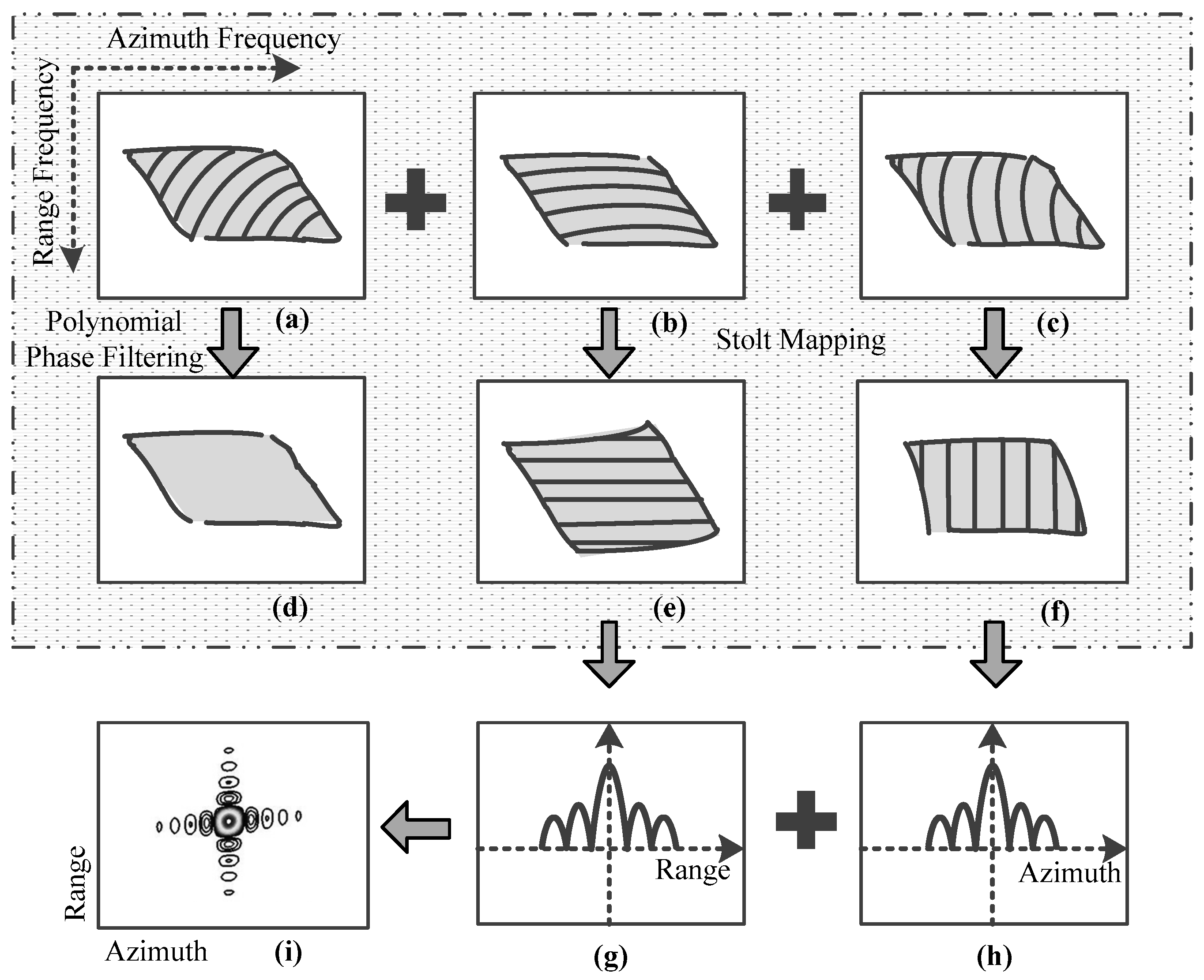
To illustrate the proposed algorithm, we consider a simple highly squinted flight geometry shown in Figure 1, with point target A. Figure 7 shows the results of the proposed algorithm by 2-D spectra of a target and the impulse response after compression. The solid lines in the first two rows represent phase contours. Figure 7a–c respectively show the support areas of 2-D cross-coupling, range, and azimuth spatially variant spectra after phase decomposition. RCM and SRC are generally very small, compared to the range bandwidth, but are exaggerated here to illustrate the effect of a target away from the reference point. The slightly curved phase contours indicate that the target is not properly focused. In Figure 7d, the phase is completely independent of range and azimuth frequencies after the polynomial phase filtering, which means that the 2-D cross-coupling spatially variant terms are eliminated entirely. The Stolt mappings of Figure 7b,c produce noticeable changes in phase contours, of which the lines are equally spaced and parallel as shown in Figure 7e,f. The echo data are well focused in range and azimuth directions respectively shown in Figure 7g,h after corresponding spatial variations being eliminated. Figure 7i shows the 2-D contour result of target.
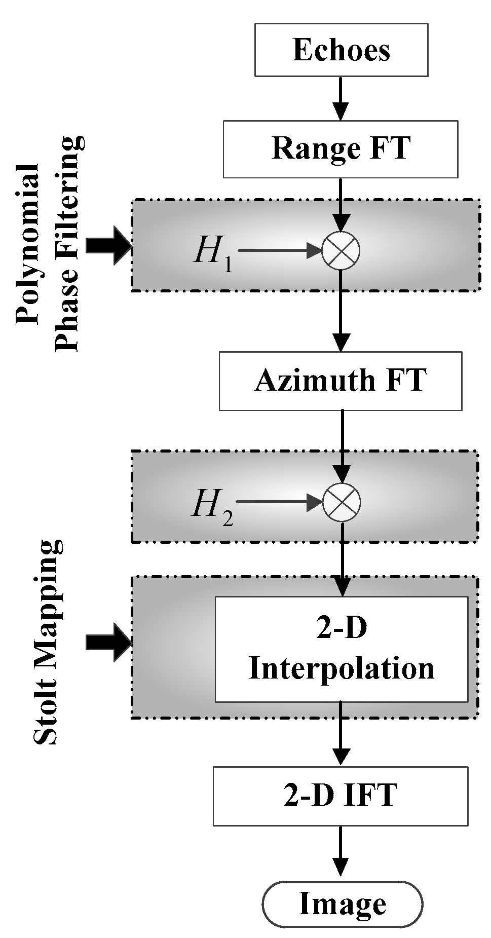
3.3. Flowchart of Imaging Algorithm
The flowchart of the imaging approach is shown in Figure 8. By using the proposed approach, spatial variations including the range, azimuth, and height spatially variant phases are greatly removed for the HRHS SAR with maneuvers. It should be noted that the range history in (1) is not a general model. When the maximum phase error between the polynomials in (1) and the real supporting points is less than , it has no impact on the imaging results. On the other hand, if the maximum phase error is larger than , the final image would be deteriorated. One solution is to take higher-order motion parameters into consideration in the proposed approach to decrease the errors. The residual phase errors can also be compensated by using the autofocus techniques which have been clearly discussed in [37,38].
4. Implementation and Discussion
4.1. Simplified Processing
According to the mapping functions in Section 3.2, if the terms in Equation (21) and in Equation (22) are sufficiently small, we can omit the corresponding interpolation to decrease the computational load of the whole imaging algorithm. In this subsection, a simplified processing method is suggested. In order to avoid the interpolation operation and to retain the image quality, the following two conditions must be satisfied
and thus the impacts on the final image could be ignored. With simulation parameters in Table 1, the maximum phase errors of Equations (25) and (26) are 0.02 and 0.7 , respectively. Clearly, the azimuth interpolation is still necessary whereas the range one is not in this case. However, the results may not be generalizable. Thus, a judgment is added in the processes to determine whether the interpolation is necessary or not according to Equations (25) and (26). The judgment flowchart is given in Figure 9.
4.2. Constraint on Scene Extent
The scene extent is analyzed in this subsection. The scene size is mainly determined by the accuracy of the proposed approach. In the focusing step, approximations only occur in the phase decomposition. According to Equation (13), the phase error is derived as
To ensure the image quality, should be less than . By computing the Taylor series expansion with respect to and ignore the higher-order terms, i.e., , can be rewritten as
where . As , we obtain the scene sizes, i.e., , in both the horizontal and vertical directions. According to Equation (28), the decomposed errors increase with the focus depths in range, azimuth, and height directions. These phase errors could have negative effects on the SAR image formation when they are larger than .
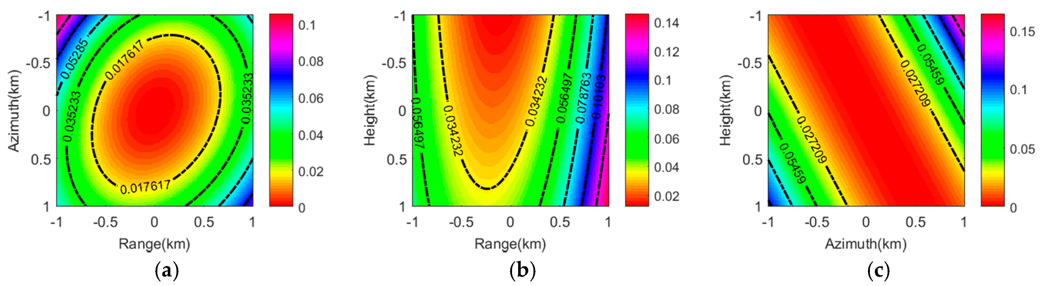
Utilizing airborne SAR simulation parameters in Table 1, Figure 10 shows the phase errors introduced by phase decompositions in range/azimuth, range/height, and azimuth/height planes. Clearly, the maximum phase errors in Figure 10a–c are all less than , which means that the residual spatial variations in range, azimuth, and height directions after focusing are small enough and thus have negligible impact on the imaging qualities.
5. Simulation Results
To prove the effectiveness of the proposed approach, simulation results are presented in this section.
5.1. Experiment 1
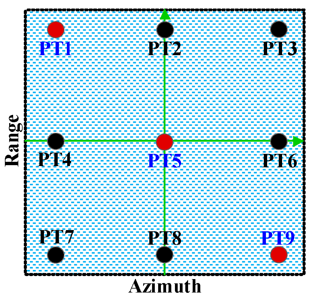
In this subsection, a spotlight mode SAR is simulated with a 3 × 3 dot-matrix being arranged in the simulation scene. The geometry of the scene is presented in Figure 11. The parameters are listed in Table 1.
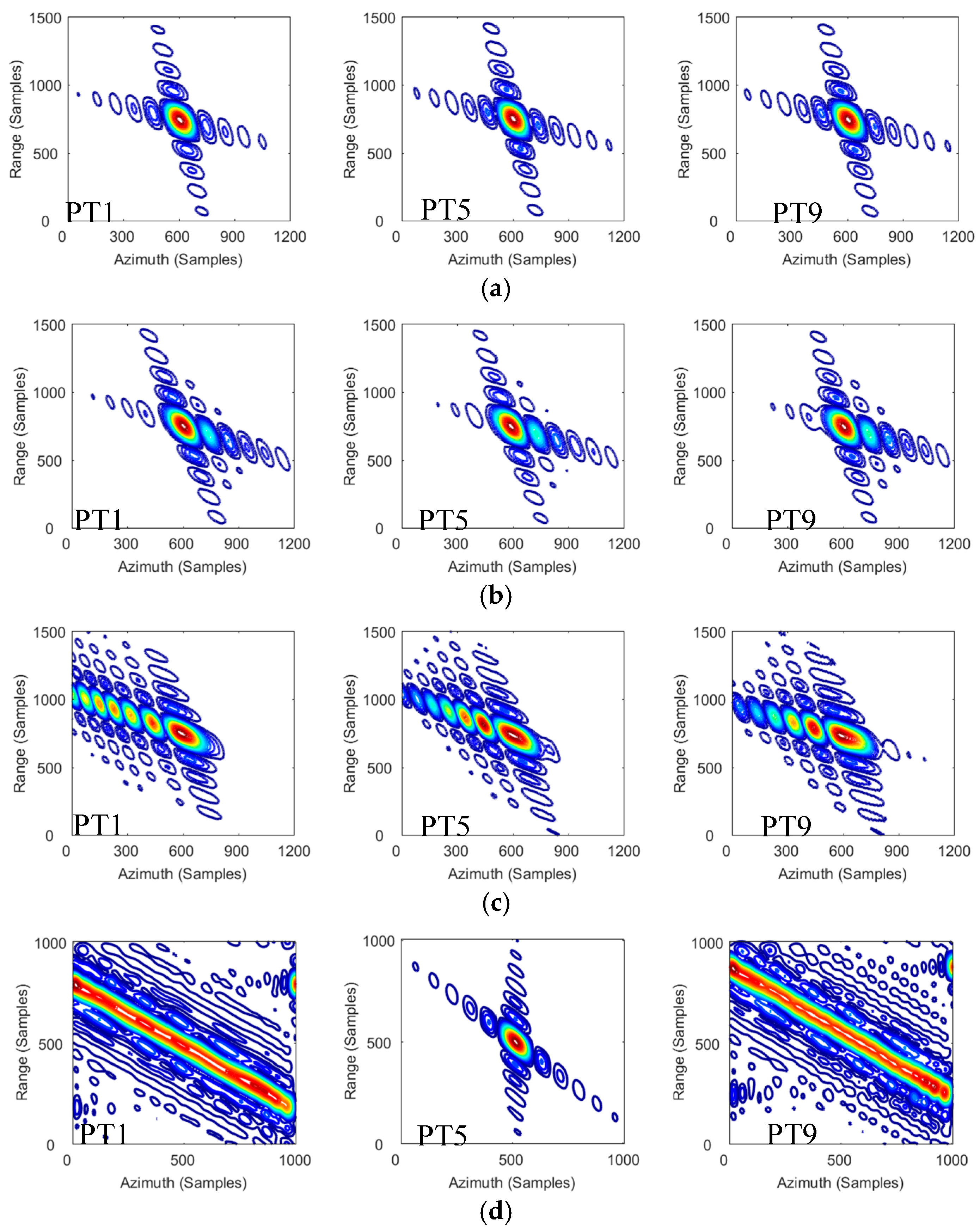
Case 1: The motion parameters , , and in this case are listed in Table 1. Simulation results without considering and are respectively used for comparisons. Moreover, the results by the FDA [16] are included. Figure 12 shows the comparative results of targets PT1, PT5, and PT9. Clearly, considering the higher-order motion parameters and , the impulse responses of targets PT1, PT5, and PT9 with different range and azimuth positions are visibly well focused by the proposed method. However, neglecting the motion parameters and , the impulse responses of targets PT1, PT5, and PT9 using the proposed method have deterioration with different degrees. The neglected parameter can degrade the near-sidelobe levels with asymmetry distortions, which means that there are deteriorations in the peak sidelobe ratio (PSLR) and integrated sidelobe ratio (ISLR), and the neglected parameter can degrade both the 3 dB width of the main lobe (i.e., the resolution) and the near-sidelobe levels, as shown in Figure 12. The impulse responses of targets PT1 and PT9 on the scene edges using FDA have deteriorations. The neglected azimuth and cross-coupling spatial variations brought by acceleration are the main causes of the problem and they increase with resolutions and scene sizes.
To quantify the precision of the proposed method, IRW, PSLR, and ISLR are used as performance measures. The results are listed in Table 2. Both the contour plots and image quality parameters demonstrate the effectiveness of the proposed method.
Case 2: In this case, , , and are set to larger values compared with those in Case 1, m/s2, m/s3, and m/s4. The ideal azimuth resolution is 0.364 m, the height of target PT9 is set to 300 m with respect to the reference target PT5, and other simulation parameters are listed in Table 1.
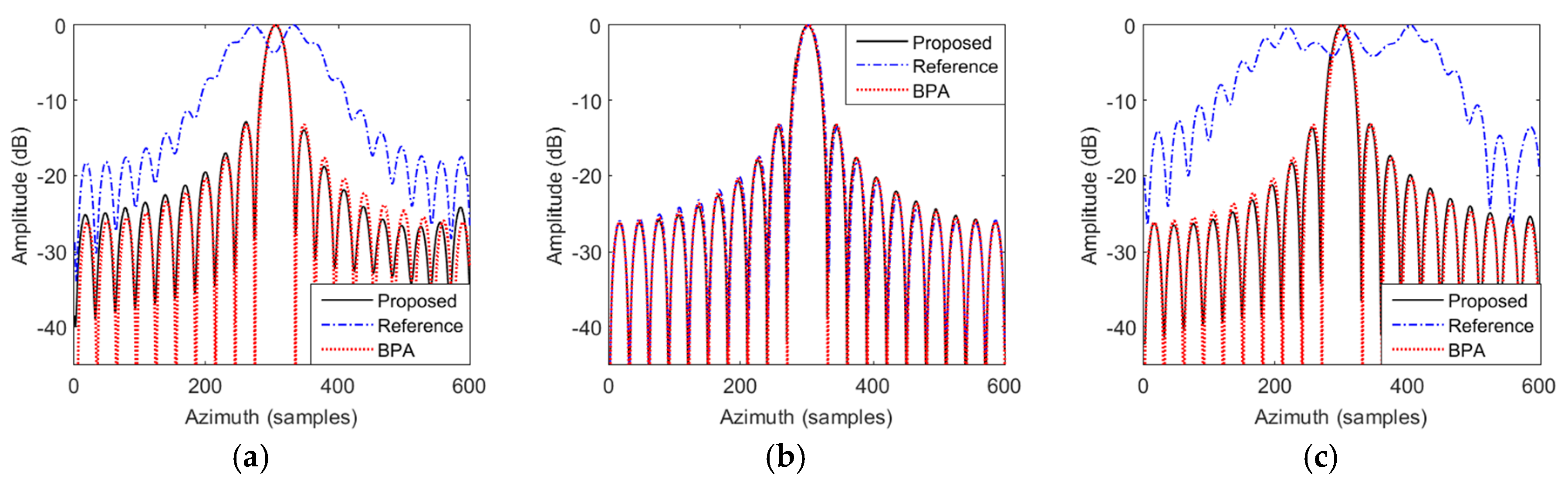
By performing the focusing method, simulation result of targets PT1, PT5, and PT9 is shown in Figure 13. The wavenumber domain algorithm [17] and BPA [29] are used for comparisons. Clearly, the results using the BPA and proposed method are visibly well focused, whereas the results on the edges achieved by [17] are not because the spatial variations introduced by the motion parameters , , and are not considered. Moreover, the target height of PT9 leads to a greater deterioration on the focused result compared with that of the flat one.
The quality parameters of azimuth point impulse responses are listed in Table 3. It is worth noting that the quality parameters of the proposed method are close to those of the BPA. In particular, the computational load of the proposed approach is much lower than that of the BPA. All these indicate that the proposed method can be well applied to the HRHS SAR with maneuvers.
5.2. Experiment 2
In the following, a comparison of the proposed approach and [17] is made. Since the highly-squinted SAR data with maneuvers are not available, a HRHS airborne SAR raw signal simulation through time domain echo generation method is performed in this subsection. The data set contains curved flight path. The carrier frequency is 35 GHz, the bandwidth of the transmitted signal is 400 MHz, reference range is 26 km, and squint angle is 63°. The scene size in range and azimuth directions are respectively 1.4 km and 1 km, and the azimuth resolution is 0.428 m. The motion parameters—namely, the velocity , acceleration , and higher-order motion parameters and are listed in Table 4. The data are focused by using the proposed approach. Moreover, a comparative focusing result of [17] is provided to demonstrate the superiority of the proposed method.
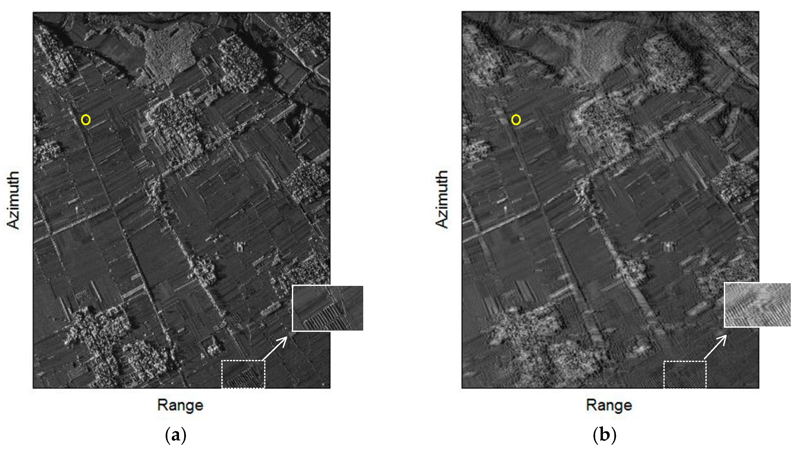
Figure 14 shows the comparative results. Clearly, the entire scene is well focused by the proposed approach, including the edge regions, as shown in Figure 14a. However, the imaging result in Figure 14b has a great deterioration in the edge regions, which are noted from the zoom-in version of the dot-line rectangle area. It is because [17] ignores the spatial variations introduced by , , and .
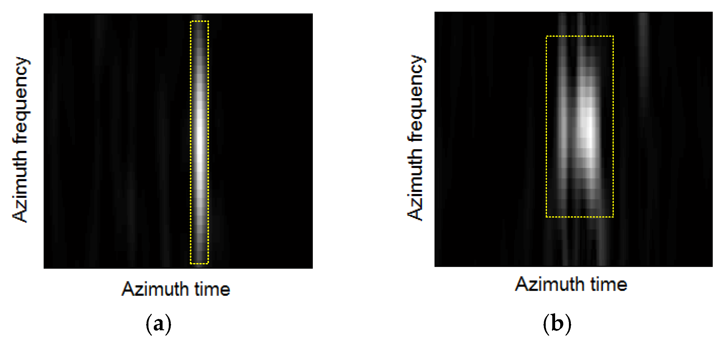
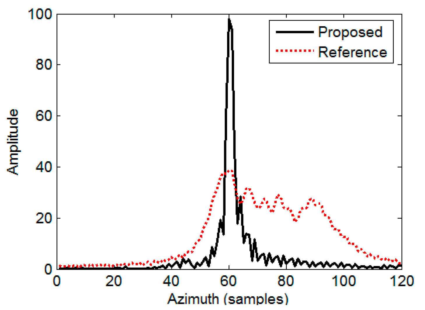
Figure 15 shows the zoom-in version of TFDs of the highlighted elliptic areas in Figure 14. The TFDs of the proposed method have a good energy aggregation, however, the TFDs of [17] have great energy dispersion. Moreover, the time-frequency resolution (TFR) of the proposed approach is higher than that of [17], which is seen from the dot-line rectangle area. It is also observed that the TFDs of the proposed approach are vertical curves while that of [17] have slight slopes. The azimuth profiles of the point in the highlighted elliptic areas are shown in Figure 16. It is evident that serious distortion and smearing occur in [17], while the proposed method provides well-focused performance. According to the above analyses, it is concluded that the proposed approach can perform well in HRHS airborne SAR with maneuvers.
6. Conclusions
SAR has been widely applied for remote sensing. However, the problems caused by the maneuvers affect the performance of traditional focusing method for the HRHS cases. In this paper, a FMPM is introduced to describe the curved path. Considering the third- and higher-order motion parameters, our analyses indicate that the spatial variations in range, azimuth, and height directions will severely impair the image quality if they are not properly accounted for during the processing. To solve this problem, we have developed a polynomial phase filter to remove the cross-coupling variations and a Stolt mapping function to the range and azimuth terms. The proposed approach is efficient, easy to implement, and can process the HRHS SAR data with maneuvers. Moreover, implementation considerations are provided. Validity and applicability are studied through theoretical analyses and numerical experiments.
Author Contributions
S.T. conceived the main idea; L.Z. and H.C.S. conceived and designed the experiments; S.T. and H.C.S. analyzed the data and wrote the paper.
Acknowledgments
This work was supported in part by the National Natural Science Foundation of China under grants 61601343 and 61671361, in part by China Postdoctoral Science Foundation Funded Project under grant 2016M600768, in part by the National Defense Foundation of China, and in part by the Fund for Foreign Scholars in University Research and Teaching Programs (the 111 project) under grant No. B18039.
Conflicts of Interest
The authors declare no conflict of interest.
Appendix A
In order to obtain the 2-D spectrum of Equation (11), we use the POSP and have
where . By using MSR [39,40,41], the stationary point is derived as
where the coefficients are
According to Equation (30), the 2-D spectrum is derived as
where , , , , and , with being the Doppler parameters of the range history, all of which are spatially variant terms. They are calculated as , , , , and .
Appendix B
For the second-order coefficient in Equation (34), we expand , , and using the Taylor series
where , , and . are the Taylor expansion coefficients. Substituting Equations (35)–(37) into leads to
where , , , , and .
For the third-order coefficient in Equation (34), is re-expanded using Taylor series with different variables as those of Equation (36)
where are the Taylor expansion coefficients. Substituting Equation (39) into , we obtain
where , , , and .
For the fourth-order coefficient in Equation (34), we substitute Equation (37) into to yield
where , , and .
Substituting Equations (38), (40), and (41) into Equation (34), we obtain the 2-D spectrum in (13). According to phase decomposition, the equations in Equation (18) are rewritten as
Their solutions are
where , , and .
References
- Cumming, I.G.; Wong, F.H. Digital Processing of Synthetic Aperture Radar Data: Algorithms and Implementation; Artech House: Norwood, MA, USA, 2005. [Google Scholar]
- Sun, G.-C.; Xing, M.; Xia, X.; Yang, J.; Wu, Y.; Bao, Z. A Unified Focusing Algorithm for Several Modes of SAR Based on FrFT. IEEE Trans. Geosci. Remote Sens. 2013, 51, 3139–3155. [Google Scholar] [CrossRef]
- Peng, X.; Wang, Y.; Hong, W.; Wu, Y. Autonomous Navigation Airborne Forward-Looking SAR High Precision Imaging with Combination of Pseudo-Polar Formatting and Overlapped Sub-Aperture Algorithm. Remote Sens. 2013, 5, 6063–6078. [Google Scholar] [CrossRef] [Green Version]
- Stroppiana, D.; Azar, R.; Calò, F.; Pepe, A.; Imperatore, P.; Boschetti, M.; Silva, J.M.N.; Brivio, P.A.; Lanari, R. Integration of Optical and SAR Data for Burned Area Mapping in Mediterranean Regions. Remote Sens. 2015, 7, 1320–1345. [Google Scholar] [CrossRef] [Green Version]
- Carrara, W.G.; Goodman, R.S.; Majewski, R.M. Spotlight Synthetic Aperture Radar: Signal Processing Algorithms; Artech House: Norwood, MA, USA, 1995. [Google Scholar]
- Ausherman, D.A.; Kozma, A.; Walker, J.L.; Jones, H.M.; Poggio, E.C. Developments in Radar Imaging. IEEE Trans. Aerosp. Electron. Syst. 1984, AES-20, 363–400. [Google Scholar] [CrossRef]
- Farrell, J.L.; Mims, J.H.; Sorrell, A. Effects of Navigation Errors in Maneuvering SAR. IEEE Trans. Aerosp. Electron. Syst. 1973, AES-9, 758–776. [Google Scholar] [CrossRef]
- Robinson, P.N. Depth of Field for SAR with Aircraft Acceleration. IEEE Trans. Aerosp. Electron. Syst. 1984, AES-20, 603–616. [Google Scholar] [CrossRef]
- Axelsson, S.R.J. Mapping Performance of Curved-path SAR. IEEE Trans. Geosci. Remote Sens. 2002, 40, 2224–2228. [Google Scholar] [CrossRef]
- Zhou, P.; Xing, M.; Xiong, T.; Wang, Y.; Zhang, L. A Variable-decoupling- and MSR-based Imaging Algorithm for a SAR of Curvilinear Orbit. IEEE Geosci. Remote Sens. Lett. 2011, 8, 1145–1149. [Google Scholar] [CrossRef]
- Eldhuset, K. A New Fourth-order Processing Algorithm for Spaceborne SAR. IEEE Trans. Aerosp. Electron. Syst. 1998, 34, 824–835. [Google Scholar] [CrossRef]
- Eldhuset, K. Ultra High Resolution Spaceborne SAR Processing with EETE4. In Proceedings of the IGARSS 2011, Vancouver, BC, Canada, 24–29 July 2011; pp. 2689–2691. [Google Scholar]
- Luo, Y.; Zhao, B.; Han, X.; Wang, R.; Song, H.; Deng, Y. A Novel High-order Range Model and Imaging Approach for High-resolution LEO SAR. IEEE Trans. Geosci. Remote Sens. 2014, 52, 3473–3485. [Google Scholar] [CrossRef]
- Wang, P.; Liu, W.; Chen, J.; Niu, M.; Yang, W. A High-order Imaging Algorithm for High-resolution Spaceborne SAR Based on a Modified Equivalent Squint Range Model. IEEE Trans. Geosci. Remote Sens. 2015, 53, 1225–1235. [Google Scholar] [CrossRef]
- Huang, L.J.; Qiu, X.L.; Hu, D.H.; Han, B.; Ding, C.B. Medium-earth-orbit SAR Focusing using Range Doppler Algorithm with Integrated Two-step Azimuth Perturbation. IEEE Geosci. Remote Sens. Lett. 2015, 12, 626–630. [Google Scholar] [CrossRef]
- Tang, S.; Zhang, L.; Guo, P.; Liu, G.; Zhang, Y.; Li, Q.; Gu, Y.; Lin, C. Processing of Monostatic SAR Data with General Configurations. IEEE Trans. Geosci. Remote Sens. 2015, 53, 6529–6546. [Google Scholar] [CrossRef]
- Li, Z.; Xing, M.; Xing, W.; Liang, Y.; Gao, Y.; Dai, B.; Hu, L.; Bao, Z. A Modified Equivalent Range Model and Wavenumber-domain Imaging Approach for High-resolution-high-squint SAR with Curved Trajectory. IEEE Trans. Geosci. Remote Sens. 2017, 55, 3721–3734. [Google Scholar] [CrossRef]
- Xing, M.; Jiang, X.; Wu, R.; Zhou, F.; Bao, Z. Motion Compensation for UAV SAR Based on Raw Radar Data. IEEE Trans. Geosci. Remote Sens. 2009, 47, 2870–2883. [Google Scholar] [CrossRef]
- Smith, A.M. A New Approach to Range-Doppler SAR Processing. Int. J. Remote Sens. 1991, 12, 235–251. [Google Scholar] [CrossRef]
- Raney, R.K.; Runge, H.; Bamler, R.; Cumming, I.G.; Wong, F.H. Precision SAR Processing using Chirp Scaling. IEEE Trans. Geosci. Remote Sens. 1994, 32, 786–799. [Google Scholar] [CrossRef]
- Cafforio, C.; Prati, C.; Rocca, F. SAR Data Focusing using Seismic Migration Techniques. IEEE Trans. Aerosp. Electron. Syst. 1991, 27, 194–207. [Google Scholar] [CrossRef]
- Tang, S.; Zhang, L.; Guo, P.; Liu, G.; Sun, G.-C. Acceleration Model Analyses and Imaging Algorithm for Highly Squinted Airborne Spotlight Mode SAR with Maneuvers. IEEE J. Sel. Top. Appl. Earth Obs. Remote Sens. 2015, 8, 1120–1131. [Google Scholar] [CrossRef]
- Li, Z.; Xing, M.; Liang, Y.; Gao, Y.; Chen, J.; Huai, Y.; Zeng, L.; Sun, G.-C.; Bao, Z. A Frequency-domain Imaging Algorithm for Highly Squinted SAR Mounted on Maneuvering Platforms with Nonlinear Trajectory. IEEE Trans. Geosci. Remote Sens. 2016, 54, 4023–4038. [Google Scholar] [CrossRef]
- Liu, G.; Li, P.; Tang, S.; Zhang, L. Focusing Highly Squinted Data with Motion Errors Based on Modified Non-linear Chirp scaling. IET Radar Sonar Navig. 2013, 7, 568–578. [Google Scholar]
- Wu, J.; Xu, Y.; Zhong, X.; Yang, J.M. A Three-Dimensional Localization Method for Multistatic SAR Based on Numerical Range-Doppler Algorithm and Entropy Minimization. Remote Sens. 2017, 9, 470. [Google Scholar] [CrossRef]
- Tang, S.; Lin, C.; Zhou, Y.; So, H.C.; Zhang, L.; Liu, Z. Processing of Long Integration Time Spaceborne SAR Data with Curved Orbit. IEEE Trans. Geosci. Remote Sens. 2018, 56, 888–904. [Google Scholar] [CrossRef]
- Wu, C.; Liu, K.Y.; Jin, M. Modeling and a Correlation Algorithm for Spaceborne SAR Signals. IEEE Trans. Aerosp. Electron. Syst. 1982, AES-18, 563–575. [Google Scholar] [CrossRef]
- Yang, L.; Zhou, S.; Zhao, L.; Xing, M. Coherent Auto-Calibration of APE and NsRCM under Fast Back-Projection Image Formation for Airborne SAR Imaging in Highly-Squint Angle. Remote Sens. 2018, 10, 321. [Google Scholar] [CrossRef]
- Munson, D.; O’Brien, J.; Jenkins, W. A Tomographic Formulation of Spotlight-mode Synthetic Aperture Radar. Proc. IEEE 1983, 71, 917–925. [Google Scholar] [CrossRef]
- Ulander, L.M.H.; Hellsten, H.; Stenström, G. Synthetic Aperture Radar Processing using Fast Factorized Back-projection. IEEE Trans. Aerosp. Electron. Syst. 2003, 39, 760–776. [Google Scholar] [CrossRef]
- Zhang, L.; Li, H.-L.; Qiao, Z.-J.; Xu, Z.-W. A Fast BP Algorithm with Wavenumber Spectrum Fusion for High-resolution Spotlight SAR Imaging. IEEE Geosci. Remote Sens. Lett. 2014, 11, 1460–1464. [Google Scholar] [CrossRef]
- Jokowartz, C.V.; Wahl, D.E.; Eichel, P.H.; Ghiglia, D.C.; Thompson, P.A. Spotlight-Mode Synthetic Aperture Radar: A Signal Processing Approach; Kluwer: Norwell, MA, USA, 1996. [Google Scholar]
- Taylor, A.E.; Mann, W.R. Advanced Calculus, 2nd ed.; John Wiley & Sons: New York, NY, USA, 1972. [Google Scholar]
- Jankech, A. Using Vluster Multifunctions for Fecomposition Theorems. Int. J. Pure Appl. Math. 2008, 46, 303–312. [Google Scholar]
- Wong, F.H.; Yeo, T.S. New Application of Nonlinear Chirp Scaling in SAR Data Processing. IEEE Trans. Geosci. Remote Sens. 2001, 39, 946–953. [Google Scholar] [CrossRef]
- An, D.; Huang, X.; Jin, T.; Zhou, Z. Extended Nonlinear Chirp Scaling Algorithm for High-resolution Highly Squint SAR Data Focusing. IEEE Trans. Geosci. Remote Sens. 2012, 50, 3595–3609. [Google Scholar] [CrossRef]
- Xu, G.; Xing, M.; Zhang, L.; Bao, Z. Robust Autofocusing Approach for Highly Squinted SAR Imagery using the Extended Wavenumber Algorithm. IEEE Trans. Geosci. Remote Sens. 2013, 51, 5031–5046. [Google Scholar] [CrossRef]
- Zhang, L.; Sheng, J.; Xing, M.; Qiao, Z.; Xiong, T.; Bao, Z. Wavenumber-domain Autofocusing for Highly Squinted UAV SAR Imagery. IEEE Sens. J. 2012, 12, 1574–1588. [Google Scholar] [CrossRef]
- Neo, Y.L.; Wong, F.; Cumming, I.G. A Two-dimensional Spectrum for Bistatic SAR Processing using Series Reversion. IEEE Geosci. Remote Sens. Lett. 2007, 4, 93–96. [Google Scholar] [CrossRef]
- Neo, Y.L.; Wong, F.; Cumming, I.G. Processing of Azimuth Invariant Bistatic SAR Data using the Range Doppler Algorithm. IEEE Trans. Geosci. Remote Sens. 2008, 46, 14–21. [Google Scholar] [CrossRef]
- Hu, C.; Liu, Z.; Long, T. An Improved CS Algorithm Based on the Curved Trajectory in Geosynchronous SAR. IEEE J. STARS 2012, 5, 795–808. [Google Scholar] [CrossRef]
Figure 1.
HRHS SAR imaging geometry with maneuvers.

Figure 2.
Impacts of motion parameter vectors
, , and on imaging results. (a) Phase errors and (b) spatially variant errors.
Figure 2.
Impacts of motion parameter vectors
, , and on imaging results. (a) Phase errors and (b) spatially variant errors.

Figure 3.
Spatial variations brought by motion parameter vectors,
, , and . (a) Range spatial variations with respect to range distance and resolution. (b) Azimuth spatially variant errors with respect to range distance and resolution.
Figure 3.
Spatial variations brought by motion parameter vectors,
, , and . (a) Range spatial variations with respect to range distance and resolution. (b) Azimuth spatially variant errors with respect to range distance and resolution.

Figure 4.
Spatial variations brought by motion parameter vectors
, , and . (a) Range spatial variations with respect to range distance and squint angle. (b) Azimuth spatially variant errors with respect to range distance and squint angle.
Figure 4.
Spatial variations brought by motion parameter vectors
, , and . (a) Range spatial variations with respect to range distance and squint angle. (b) Azimuth spatially variant errors with respect to range distance and squint angle.

Figure 5.
Spatial variations distribution. (a) Spatial variations distributed in ground scene. (b) TFDs of targets T0, T1, T2, and T3.
Figure 5.
Spatial variations distribution. (a) Spatial variations distributed in ground scene. (b) TFDs of targets T0, T1, T2, and T3.

Figure 6.
Illustration of cross-coupling spatial variation elimination by TFDs of three targets with different positions. (a,b) TFDs before and after bulk compensation, respectively; (c,d) TFDs before and after polynomial phase filtering.
Figure 6.
Illustration of cross-coupling spatial variation elimination by TFDs of three targets with different positions. (a,b) TFDs before and after bulk compensation, respectively; (c,d) TFDs before and after polynomial phase filtering.

Figure 7.
Illustration of proposed algorithm by 2-D spectra of a target and impulse response after compression. (a–c) in top row are 2-D spectra after phase decomposition, while (d–f) in the second row illustrate 2-D spectra after corresponding processing, and (g–i) in the bottom row are imaging results. The solid lines in the first two rows represent phase contours.

Figure 8.
Flowchart of the proposed algorithm.

Figure 9.
Judgment flowchart of the interpolation.

Figure 10.
Phase errors in (a) range and azimuth, (b) range and height, and (c) azimuth and height planes.
Figure 10.
Phase errors in (a) range and azimuth, (b) range and height, and (c) azimuth and height planes.

Figure 11.
Ground scene for simulation.

Figure 12.
Comparative results of target PT1, PT5, and PT9. (a) Proposed method, (b) c not considered, (c) b not considered, and (d) FDA.
Figure 12.
Comparative results of target PT1, PT5, and PT9. (a) Proposed method, (b) c not considered, (c) b not considered, and (d) FDA.

Figure 13.
Comparative results of azimuth point impulse responses processed by proposed method [17], and BPA. (a) Target PT1. (b) Target PT5. (c) Target PT9.
Figure 13.
Comparative results of azimuth point impulse responses processed by proposed method [17], and BPA. (a) Target PT1. (b) Target PT5. (c) Target PT9.

Figure 14.
Imaging results (a) by proposed approach and (b) [17].
Figure 14.
Imaging results (a) by proposed approach and (b) [17].

Figure 15.
TFDs of rectangular domain in Figure 14. (a) Using the proposed approach. (b) Using [17].

Figure 16.
Comparison of azimuth pulse response.


Table 1.
Parameter settings.
| Motion Parameter | Value | System Parameter | Value |
|---|---|---|---|
| Radar Position at ACM | (0, 0, 10) km | Carrier Frequency | 17 GHz |
| Reference Position | (12.68, 26, 0) km | Pulse Bandwidth | 500 MHz |
| Velocity | (0, 170, −10) m/s | Sampling Frequency | 620 MHz |
| Acceleration | (1.2, 1.73, −1.4) m/s2 | Squint Angle | 60° |
| Third-order Parameter | (−0.09, 0.11, −0.14) m/s3 | Azimuth Resolution | 0.242 m |
| Fourth-order Parameter | (0.005, 0.007, 0.003) m/s4 | Scene Size (Range×Azimuth) | 1.6 × 1.6 km |
Table 2.
Image quality parameters.
| Range | Azimuth | ||||||
|---|---|---|---|---|---|---|---|
| Method | Target | IRW (m) | PSLR (dB) | ISLR (dB) | IRW (m) | PSLR (dB) | ISLR (dB) |
| Proposed | PT1 | 0.266 | −13.21 | −9.99 | 0.247 | −13.17 | −9.92 |
| PT5 | 0.265 | −13.23 | −10.01 | 0.243 | −13.22 | −10.03 | |
| PT9 | 0.266 | −13.19 | −9.98 | 0.241 | −13.15 | −9.95 | |
| FDA | PT1 | 0.266 | −13.24 | −9.96 | 0.893 | −6.02 | −4.49 |
| PT5 | 0.266 | −13.25 | −10.09 | 0.242 | −13.23 | −10.07 | |
| PT9 | 0.267 | −13.17 | −10.01 | 1.302 | −4.74 | −3.56 | |
Table 3.
Image quality parameters.
| Method | Target | IRW (m) | PSLR (dB) | ISLR (dB) |
|---|---|---|---|---|
| Proposed | PT1 | 0.367 | −13.16 | −9.87 |
| PT5 | 0.365 | −13.21 | −10.02 | |
| PT9 | 0.362 | −13.14 | −9.94 | |
| [17] | PT1 | 1.031 | −6.11 | −4.56 |
| PT5 | 0.364 | −13.24 | −10.06 | |
| PT9 | 1.135 | −5.78 | −4.12 | |
| BPA | PT1 | 0.365 | −13.24 | −10.04 |
| PT5 | 0.364 | −13.27 | −10.08 | |
| PT9 | 0.361 | −13.25 | −10.05 |
Table 4.
Motion parameter settings.
| Motion Parameter | Value |
|---|---|
| Velocity | (0, 110, −10) m/s |
| Acceleration | (1.21, 1.43, −0.74) m/s2 |
| 3rd-order Paramater | (−0.1, 0.2, 0.2) m/s3 |
| 4th-order Paramater | (0.007, −0.015, 0.004) m/s4 |
© 2018 by the authors. Licensee MDPI, Basel, Switzerland. This article is an open access article distributed under the terms and conditions of the Creative Commons Attribution (CC BY) license (http://creativecommons.org/licenses/by/4.0/).
Share and Cite
MDPI and ACS Style
Tang, S.; Zhang, L.; So, H.C. Focusing High-Resolution Highly-Squinted Airborne SAR Data with Maneuvers. Remote Sens. 2018, 10, 862. https://doi.org/10.3390/rs10060862
AMA Style
Tang S, Zhang L, So HC. Focusing High-Resolution Highly-Squinted Airborne SAR Data with Maneuvers. Remote Sensing. 2018; 10(6):862. https://doi.org/10.3390/rs10060862
Chicago/Turabian StyleTang, Shiyang, Linrang Zhang, and Hing Cheung So. 2018. "Focusing High-Resolution Highly-Squinted Airborne SAR Data with Maneuvers" Remote Sensing 10, no. 6: 862. https://doi.org/10.3390/rs10060862
Note that from the first issue of 2016, this journal uses article numbers instead of page numbers. See further details here.