Satellite Images and Gaussian Parameterization for an Extensive Analysis of Urban Heat Islands in Thailand


1
Department of Computer Science, Khon Kaen University, Khon Kaen 40002, Thailand
2
Department of Engineering, University of Perugia, via Duranti 93, 06125 Perugia, Italy
*
Author to whom correspondence should be addressed.
Remote Sens. 2018, 10(5), 665; https://doi.org/10.3390/rs10050665
Submission received: 23 March 2018
/
Revised: 16 April 2018
/
Accepted: 21 April 2018
/
Published: 24 April 2018
(This article belongs to the Special Issue Urban Heat Island Remote Sensing)
Abstract
:For the first time, an extensive study of the surface urban heat island (SUHI) in Thailand’s six major cities is reported, using 728 MODIS (MODerate Resolution Imaging Spectroradiometer) images for each city. The SUHI analysis was performed at three timescales—diurnal, seasonal, and multiyear. The diurnal variation is represented by the four MODIS passages (10:00, 14:00, 22:00, and 02:00 local time) and the seasonal variation by summer and winter maps, with images covering a 14-year interval (2003–2016). Also, 126 Landsat scenes were processed to classify and map land cover changes for each city. To analyze and compare the SUHI patterns, a least-square Gaussian fitting method has been applied and the corresponding empirical metrics quantified. Such an approach represents, when applicable, an efficient quantitative tool to perform comparisons that a visual inspection of a great number of maps would not allow. Results point out that SUHI does not show significant seasonality differences, while SUHI in the daytime is a more evident phenomenon with respect to nighttime, mainly due to solar forcing and intense human activities and traffic. Across the 14 years, the biggest city, Bangkok, shows the highest SUHI maximum intensities during daytime, with values ranging between 4 °C and 6 °C; during nighttime, the intensities are rather similar for all the six cities, between 1 °C and 2 °C. However, these maximum intensities are not correlated with the urban growth over the years. For each city, the SUHI spatial extension represented by the Gaussian footprint is generally not affected by the urban area sprawl across the years, except for Bangkok and Chiang Mai, whose daytime SUHI footprints show a slight increase over the years. Orientation angle and central location of the fitted surface also provide information on the SUHI layout in relation to the land use of the urban texture.
1. Introduction
Urban heating is usually quantified by means of the urban heat island (UHI), a well-known anthropogenic thermal modification whose effects have implications for human comfort and health, ecosystem function, local weather, air pollution, urban planning, and energy management [1,2,3,4]. The UHI phenomenon is linked to urban land transformations, especially when vegetated and rural zones are substituted by impervious surfaces, causing an increase in sensible heat flux and a decrease in latent heat in urban areas [5]. Urban heating is mainly ascribed to the trapping and absorption of solar irradiation in built-up areas connected to the thermal capacity of construction materials and the urban canyon phenomenon [6]. As a result, a difference in air and surface temperature between urban area and rural surroundings arises [7], quantified as UHI intensity or magnitude.
Many studies have estimated the UHI intensity by using ground-based weather stations observing air temperature in urban and rural locations [8], however, the sparsely distributed stations do not allow a global view over the urban area. Air temperature has a diurnal cycle with a nighttime UHI formation, while surface temperatures typically exhibit a surface urban heat island (SUHI) throughout the diurnal cycle, with a maximum in the daytime [9,10,11].
Advances in space-based remote sensing and satellite data availability have contributed to the growing number of studies on SUHI in several cities around the world, exploiting the global spatial coverage and the revisit time of satellite remote sensing missions [12]. SUHI map images were extensively retrieved by using Landsat data, providing spatiotemporal analysis and allowing the modeling of the urban thermal patterns with the land cover classes [13,14,15]. The MODerate Resolution Imaging Spectroradiometer (MODIS), aboard Terra and Aqua satellites, allows monitoring SUHI daily variations but with a lower spatial resolution (1 km) [16,17,18].
SUHI mapping can also satisfy the growing demand for integrating urban planning and landscape ecosystems, supplying scientific support for urban development policies [19]. In this context, remotely sensed imagery is often used to map impervious surfaces together with SUHI, the former widely recognized as a significant urbanization indicator affecting the thermal pattern. Instead, it is well known that the increase of vegetation and green spaces in the urban texture is one of the main strategies to mitigate SUHI intensity [20,21].
In this work, we provide a SUHI insight on different Thailand urban areas. Even though a great number of papers have explored the SUHI maps retrieved by remote sensing data in several cities worldwide, a complete study in Thailand is missing. For instance, different works were carried out with ground-based weather stations measuring air temperature, including: investigation of the UHI intensity in three big cities in Thailand (Bangkok, Chiang Mai and Songkhla) by using meteorological weather stations for the period 2004–2008 [22]; analysis of the air temperature data from four weather stations for a UHI insight in Bangkok area [23,24]. Spaceborne imagery in Thailand was used with limited spatial and temporal coverage: study of the land surface temperature (LST) pattern in Chiang Mai city (northern Thailand) with only two Landsat Enhanced Thematic Mapper Plus (ETM+) images (one in 2000 and one in 2006) [25]; Kantarawichai district analysis in the northeastern Thailand with only two Landsat images (one in 2006 and one in 2009) [26]; SUHI monitoring on Bangkok with few MODIS images in the period 2001–2003 [27]. Recently, a SUHI insight over the land use zoning plan of Bangkok using seven Landsat 8 scenes was proposed [28].
To bridge this gap, this work provides, for the first time, an extensive temporal and spatial investigation in Thailand by examining the SUHI of six major cities located in different geographic regions during a long-time interval (2003–2016) using 728 MODIS images, allowing daytime and nighttime monitoring. Also, 126 Landsat scenes were processed to classify and map land-cover changes in each city. Since Thailand has experienced significant changes in urban development during the last 20 years, this study points out the spatiotemporal SUHI trend for each city and intercity (trend among cities) and performs a comparison with the built-up surface growth derived from Landsat imagery.
To examine the SUHI patterns and their relevance in terms of temporal and spatial trends, empirical metrics were retrieved to quantify the phenomenon and to perform comparative analyses. The study was carried out by means of a two-dimensional least-square Gaussian fitting technique, whose parameterization and visualization proves to be useful in SUHI pattern insight.
2. Study Area
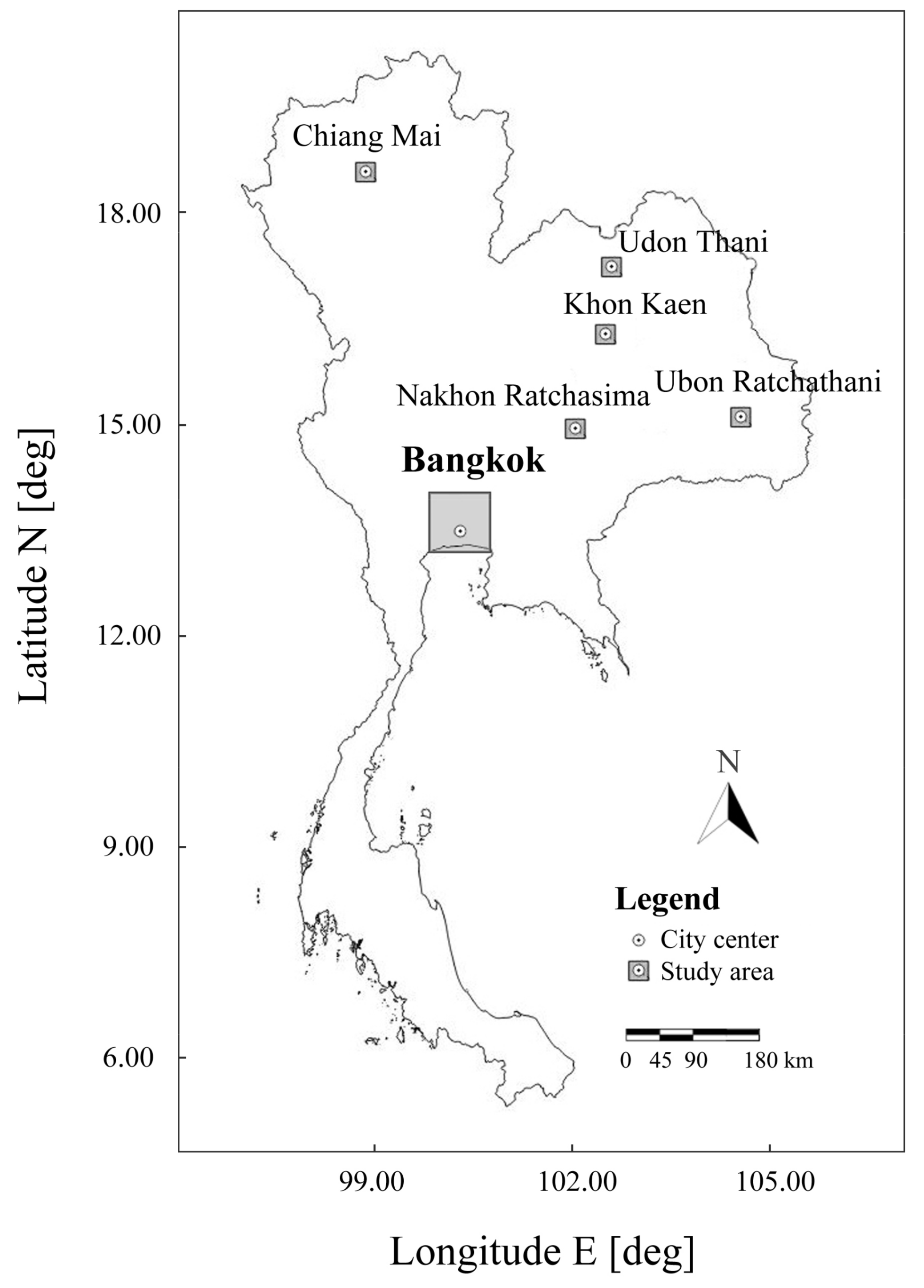
Six major cities in Thailand were selected for this study (Figure 1), including: (1) Bangkok (BG), the capital of Thailand, located in the central region; (2) Chiang Mai (CM), the largest city in the northern region, and four large cities located in northeastern region: (3) Nakhon Ratchasima (NR); (4) Ubon Ratchathani (UR); (5) Khon Kaen (KK); and (6) Udon Thani (UT).
Bangkok has a population of about 6.3 million within municipality and the largest urban extension in Thailand. It is located in the Chao Phraya River delta in Thailand central plains. The area is flat and low-laying, with a mean elevation of 1.5 m above sea level. It has a tropical wet and dry climate with three seasons—namely, summer, rainy season, and winter. The air temperature ranges from an average value of 22.0 °C in December to 35.4 °C in April. The rainy season begins around mid-May until October, with the dry and cool northeast monsoon occurring until February, when the summer season starts until mid-May.
Chiang Mai (136,700 inhabitants within municipality) is the capital of Chiang Mai Province, situated at about 300 m above sea level, 696 km north of Bangkok. About 70% of the Chiang Mai province consists of mountains covered with forests. The coolest months are December and January. The temperature throughout the year varies between 14 and 30 °C, with an average value of 26 °C.
Finally, four of the largest cities located in the northeastern Thailand were selected: Nakhon Ratchasima (135,300 inhabitants within municipality), Ubon Ratchathani (82,800), Khon Kaen (110,000), and Udon Thani (135,500). They are located mostly in flat plains between latitudes 14°0′E and 18°30′N and longitudes 101°0′E and 105°0′E. Average temperatures range from 19.6 °C to 30.2 °C. Northeastern Thailand is the focal point of the Greater Mekong Subregion, which operates as an economic center with Laos, China (Yunnan), and Vietnam. Development projects at large scales have sprung up, including construction of highways to provide access to the northeastern Thailand area for trade increasing. All of these aspects have expanded the northeastern economy and fostered rapid growth of the urban territories.
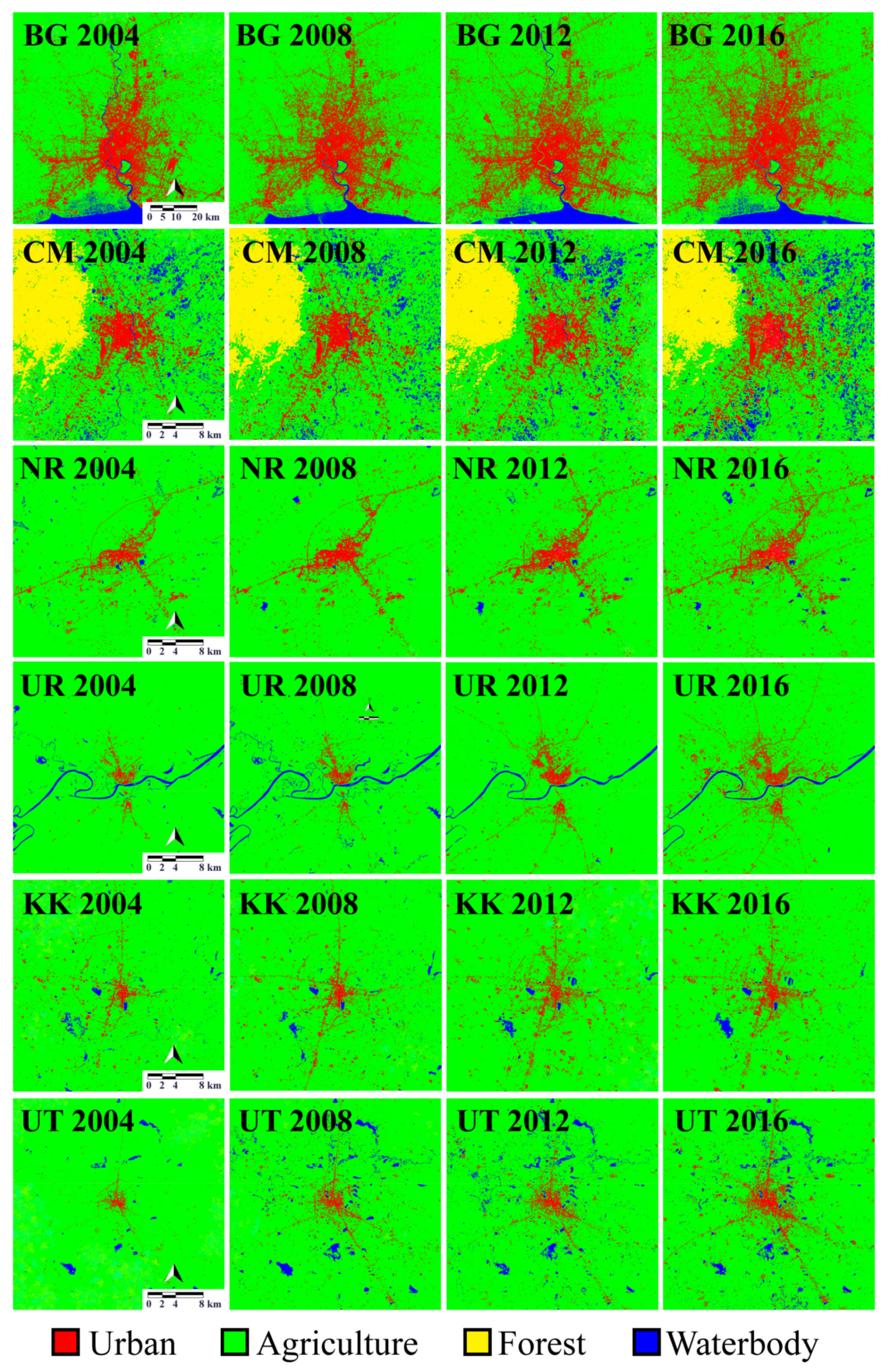
Figure 2 shows the urban surface evolution for the six cities in the years 2004, 2008, 2012, and 2016. These maps have been obtained from Landsat images as described in Section 3.1. The overview of Figure 2 shows the urban expansion across the years, which makes the study of the surface thermal impact interesting in terms of spatial and temporal evolution. Concerning the land use of urban areas for the six cities, the city core always includes high- and medium-density residential areas, commercial zones, and government institutes, while outskirts are mainly made up of medium- and low-density residential areas and industrial zones.
3. Data and Methods
3.1. Satellite Data
Land surface temperature (LST) images retrieved from observations of the MODIS sensors on board Terra and Aqua satellites were used. LST data were downloaded from ORNL DAAC archive [29], selecting MOD11A2 (Terra) and MYD11A2 (Aqua) 8-day LST products with 1 km resolution. These LST products are composed of daily 1 km LST values averaged during an 8-day period; cloudy pixels for each image were masked out. Terra satellite passes over Thailand at around 10:00 am and 22:00 (local time), whilst Aqua satellite passes at around 14:00 and 2:00 am; local time is +7:00 from UTC time. In this work, observations from 2003 until the end of 2016 were selected.
Since Thailand is in the tropical zone and has very few cloud-free images during the rainy/monsoon season, in this study, satellite LST images during two intervals within each year were acquired: three months during winter (November–January) and summer (February–April), excluding the six rainy months (May–October). Overall, 336 daytime and 392 nighttime MODIS-Terra/Aqua LST images were processed for a total of 728 raster LST maps of 1 km spatial resolution for each city.
Therefore, the whole dataset will allow an analysis of the SUHI temporal variation at three timescales: diurnal, seasonal, and multiyear. The diurnal variation is represented by the four times that MODIS passes (daytime: 10:00 and 14:00; nighttime: 22:00 and 02:00), while the seasonal variation is examined by comparing the summer and winter maps. Overall, all the selected images (24 in summer and 28 in winter for each city and for each year) were averaged to get seasonal LST mean values (i.e., winter and summer separately) at the four diurnal times, from which the SUHI was extracted.
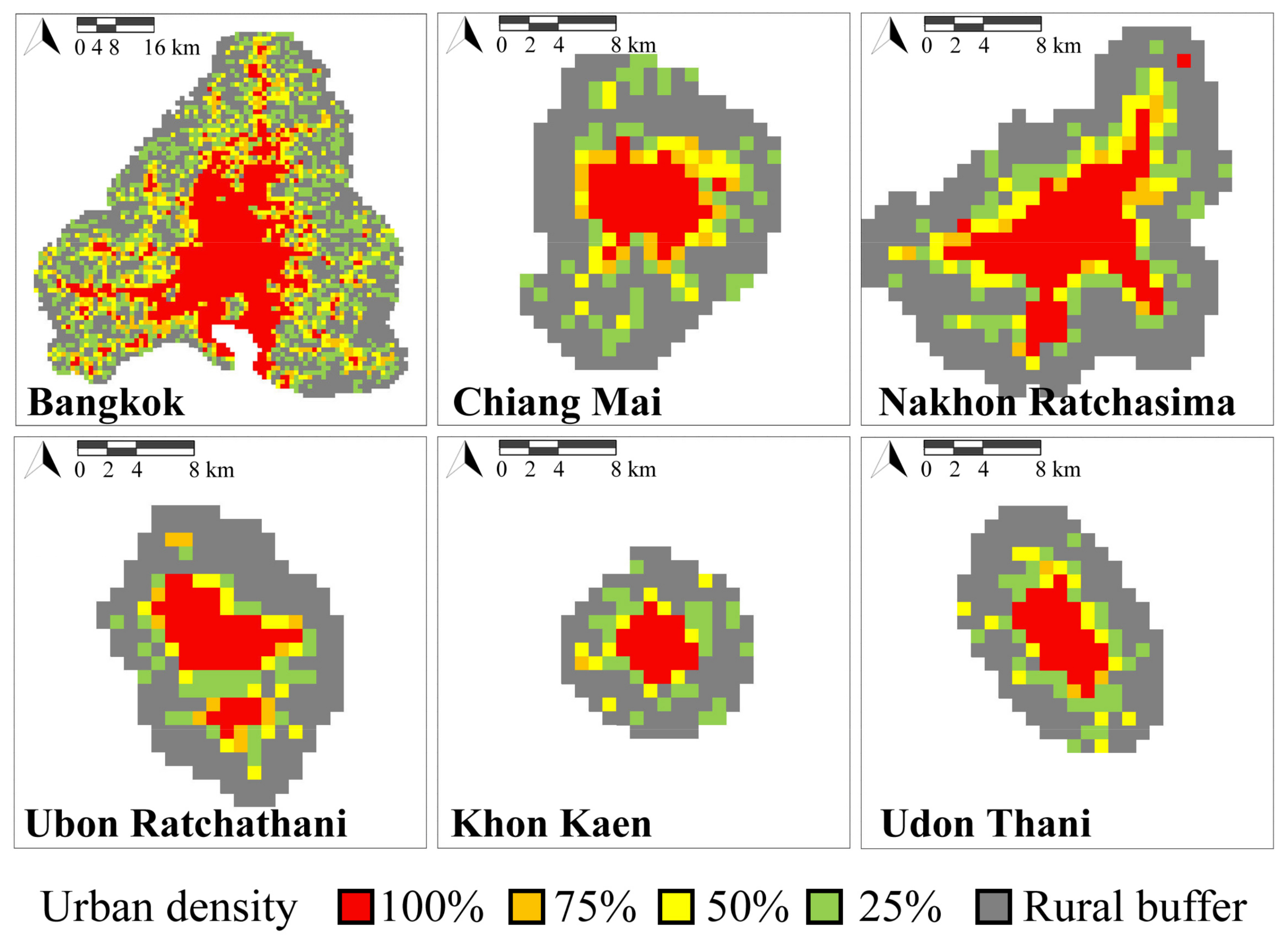
To identify the rural buffer for the SUHI computation, MODIS Land Cover Type Product (MCD12Q1) with 500 m spatial resolution was used. The MCD12Q1 products yearly categorize the land using combined Terra and Aqua MODIS observations to identify different land cover classes.
Land use and land cover (LULC) maps for each city were also derived from cloud-free Landsat-4/Landsat-5 Thematic Mapper (TM), Landsat-7 Enhanced Thematic Mapper Plus (ETM+), and Landsat-8 Operational Land Imager (OLI) images with a spatial resolution of 30 m downloaded from USGS archive [30]. A total of 126 scenes from 2003 to 2016 were used to extract the urban area extent, exploiting the higher spatial resolution with respect to the MCD12Q1 products. The land covers were classified into four broad types (i.e., built-up land, water body, agriculture, and forest, Figure 2) applying a supervised maximum likelihood classification approach [31,32]. The user and producer accuracy [33] for urban and agriculture classes—evaluated by high-resolution images incorporated in GoogleEarth Pro® and reported as mean value over all the Landsat maps—are as follows: user (urban) = 0.80; user (agriculture) = 0.94; producer (urban) = 0.95; producer (agriculture) = 0.84.
3.2. Estimation of the SUHI
The SUHI intensity quantifies the heating effects in an urban area, and we computed it as the surface temperature difference between urban (LSTURB) and rural (LSTRUR) pixels:
SUHI = LSTURB − LSTRUR.
The reference LSTRUR represents the mean of LST values associated with the rural pixels in a buffer area, surrounding the urban area, of about 3 km. In such buffer rural areas, water pixels were discarded. The choice of the 3 km buffer is a trade-off that allows, for all the cities, to discard high-altitude rural zones (e.g., Chiang Mai forest in Figure 2) that would lower the LST rural bias. For the computation of Equation (1), to discern built-up and rural pixels at the LST spatial resolution (1 km), urban and rural categories were extracted from the MCD12Q1 product. Figure 3 shows an example of these reference maps for the six cities for 2013, resampled at 1 km pixel size from the native 500 m, used for the computation of the reference LSTRUR.
The thermal characterization of an urban area by means of SUHI maps is also appropriate for comparative analysis among different cities because SUHI intensity is not an absolute temperature, but a temperature difference between rural and urban areas. Therefore, the effects of local weather conditions and other error sources are dampened.
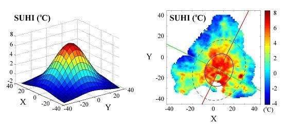
To perform SUHI pattern comparisons, a technique based on a two-dimensional least-square Gaussian fit of the heat island was applied. This SUHI fitting technique was proposed in [34] and applied in [10,13,27,35,36,37]. The 2D Gaussian surface can be a useful representation of the SUHI pattern when an urban area shows a clear heat island with respect to the rural surroundings, especially if clustered SUHI values are prone to decrease towards the map boundary. The Gaussian fitting of the spatially distributed SUHI(x, y) (°C) obtained from MODIS data is described as follows:
where (x, y) (km) is the pixel location in the map, with the origin (0, 0) in the center of the map. From Equation (2), a nonlinear data-fitting in least-squares sense was performed [35] in order to estimate:
- -
- the magnitude a0 (°C) of the SUHI maximum intensity of the study area;
- -
- the spatial extent (ax, ay) (km), central location (x0, y0) (km), and orientation (φ) (degree) of the SUHI pattern.
A correlation coefficient (r) between the SUHI map from MODIS data and the fitted Gaussian surface was computed to assess the capability of the fitting surface to follow the actual pattern. The two parameters, ax and ay (spatial extent), were also combined to define the overall area of the SUHI. Such an area or footprint is an ellipse obtained by horizontally cross-sectioning the Gaussian surface. The ellipse axes are ax and ay, φ is the orientation angle, with the maximum SUHI value located in the footprint center x0, y0.
The ellipse area defined by the distance from the center, where SUHI decreases to 61% (e−1/2) with respect to the maximum value a0, will be defined as Ar61% (km2). Similarly, a footprint area where SUHI is greater than a fixed threshold can be defined—for example, greater than 1 °C (Ar1C) [10,34].
This fitting technique works well for urban areas with regular shapes. The method is suitable for large-area analysis by satellite data of spatial resolution like MODIS. Since the fitting provides a smoothed surface, the greater variability of higher spatial resolution images (e.g., Landsat maps) reduces the correlation coefficient and the representativeness of the Gaussian footprints [35].
4. Results and Discussion
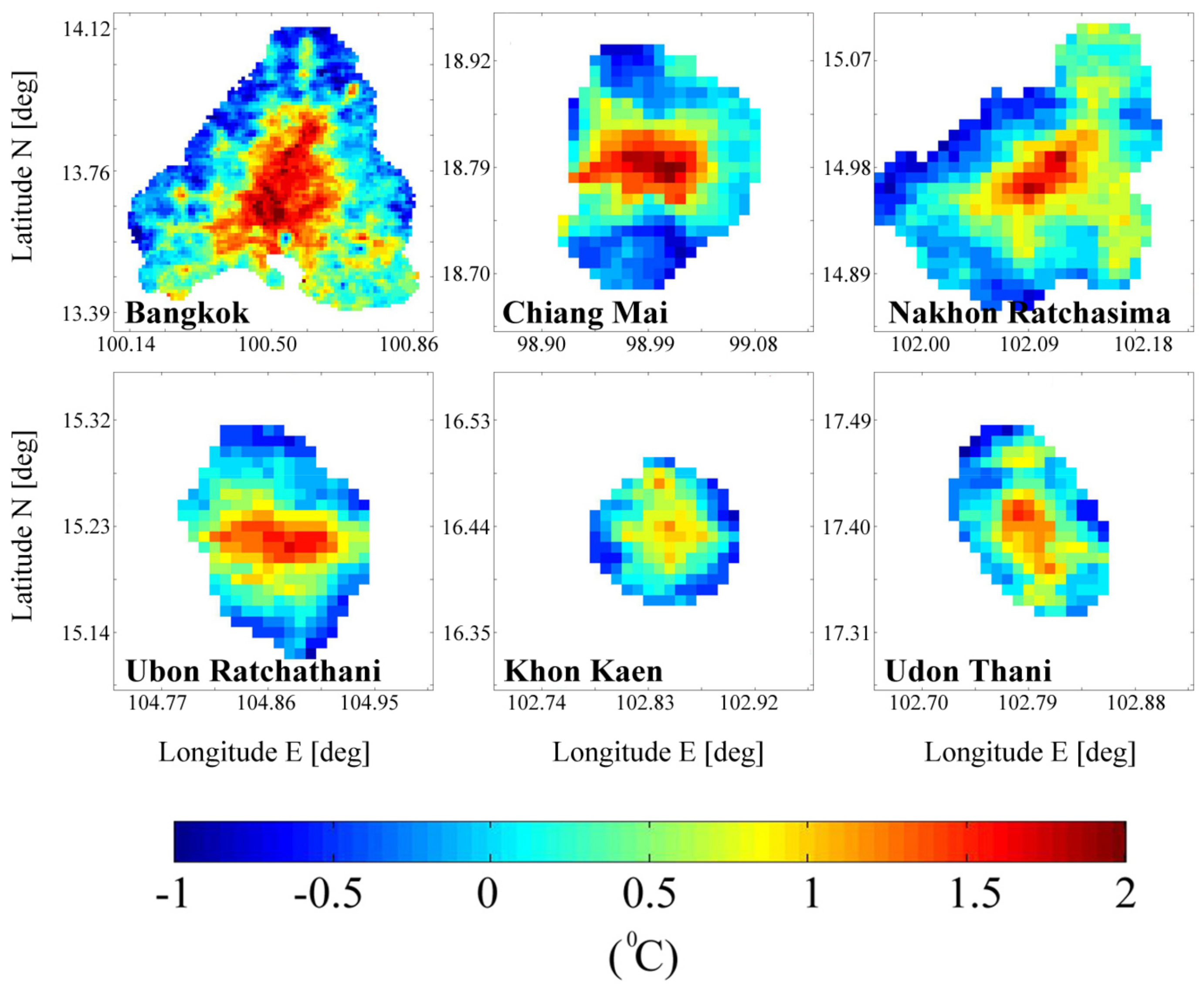
The spatial trend of the SUHI pattern was analyzed at three timescales (diurnal, seasonal, and multiyear), considering the trend for each city and comparing the trend for all the six cities (intercity analysis). These SUHI patterns were examined during a 14-year interval (2003–2016): for example, the SUHI during 2013 for the six cities is shown in Figure 4 considering the summer season at 22:00.
The example of Figure 4 shows that the nighttime urban heating is not too pronounced—that is, few degrees with respect to rural area. In the next subsections, the use of the Gaussian parameterization will allow us to have a SUHI trend overview and to perform comparisons that a simple visual inspection of a great number of maps would not allow.
4.1. Gaussian Fitting of SUHI Maps
As discussed in Section 3.2, the 2D Gaussian surface can be a useful representation of the SUHI pattern when an urban area shows a clear and clustered heat island decreasing towards the rural area. Some situations (anomalous spotted rural heating or negligible temperature differences between LSTURB and LSTRUR) can lead to a low correlation coefficient r between the SUHI maps from MODIS data and the fitted Gaussian surface. Table 1 describes the capability of the fitting surface to follow the actual SUHI pattern, reporting the r mean value for the years 2003–2016. We have considered the fitting reliable when is greater than 0.6 and the Gaussian footprint covers the urban area.
Table 1 shows that some combinations of city–season–hour do not have a robust fit. An explanation will be provided in the successive Figure 5 and Figure 6 by examining the correspondent SUHI patterns. The correlation is always better for the summer nighttime fitting with respect to the summer daytime, whereas the same is not confirmed for the winter. Considering the whole daily cycle, Chiang May has the best performance in terms of correlation.
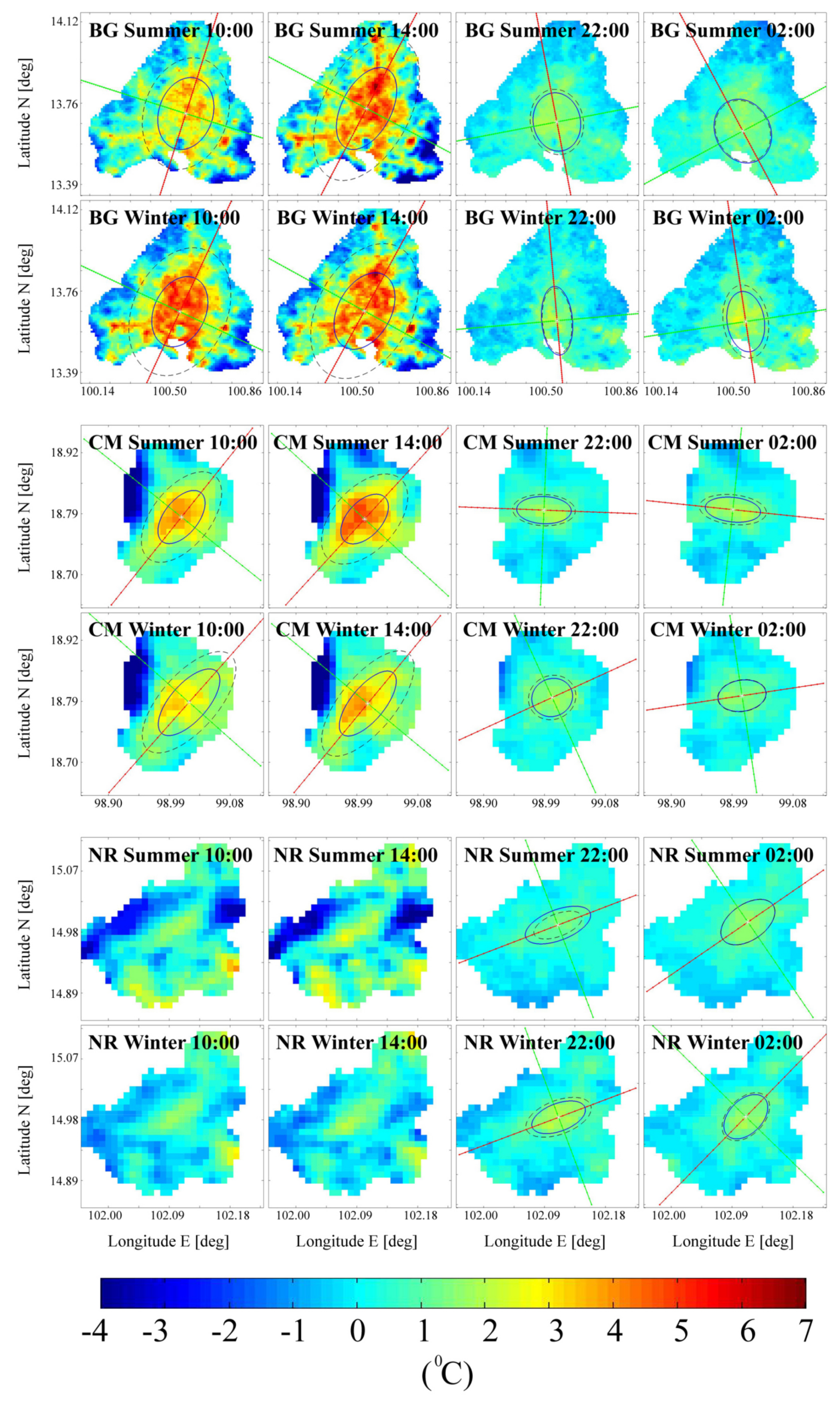
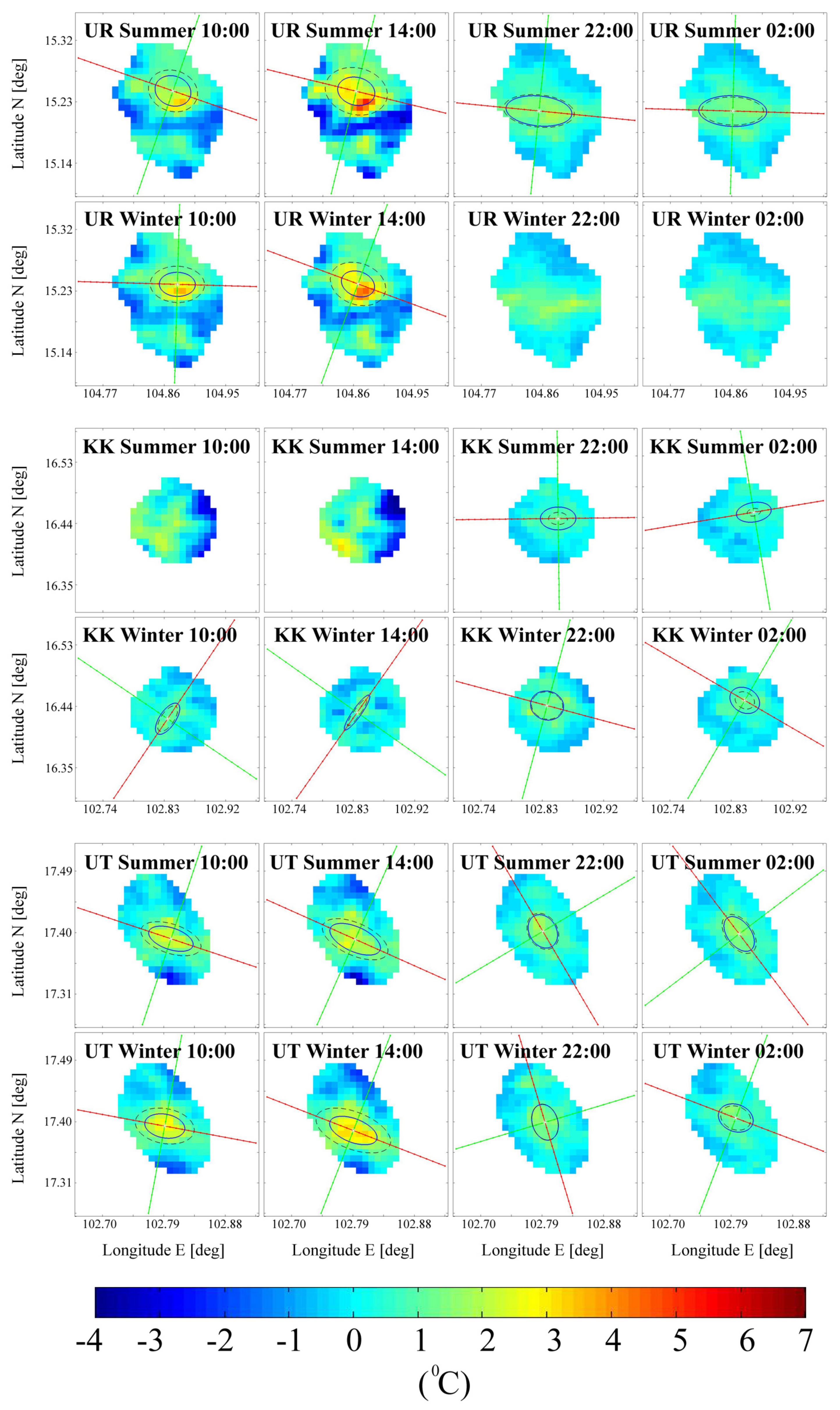
Figure 5 and Figure 6 show the SUHI maps and the correspondent Gaussian fitting for the six cities during 2014 both in summer and winter, reporting also the diurnal variation at 10:00, 14:00, 22:00, and 02:00. Each SUHI(x, y) pattern from MODIS data—with x and y representing the latitude and longitude—were fitted with a Gaussian surface and the descriptive parameters collected. In Figure 5 and Figure 6, the black continuous ellipse superimposed on the maps represents the footprint area Ar61%, while the black dashed ellipse represents Ar1C. The red and green straight lines correspond to the directions of the ellipse’s major and minor axes, the former also defining the orientation angle φ. The intersection point of the two lines (i.e., the footprint center) is the central location (x0, y0), expressed as shift from the center of the map (0, 0). For example, with reference to the first panel of Figure 5 (BG Summer 10:00), Ar61% = 755.6 km2, Ar1C = 1815.7 km2, φ = 72.3° (i.e., along the north–east and south–west (NE–SW) quarters) and (x0, y0) = (7.3, −5.5) km; the estimated magnitude a0 is 3.4 °C. The Gaussian fitting procedure is not generally conditioned by localized surface temperature peaks within the pattern, being prone to smooth such isolated thermal discontinuities.
As a general overview of Figure 5 and Figure 6, the daytime SUHI is a more evident phenomenon with respect to the nighttime one, while summer and winter SUHIs at the same hour are quite similar. At nighttime periods, due to the absence of solar forcing and the reduced working activities and traffic, the urban heat island intensity decreases, since rural and urban temperatures tend to get closer. The exceptions are NR and KK, since their daytime SUHI intensities are similar to those at night in the urban area. Particularly, KK, one of the six cities with the smallest urban size, always exhibits a very weak urban heating with respect to rural surroundings. Ar61% and Ar1C, clearly distinct during daytime, are almost the same at night. In some cases, Ar1C is inside Ar61% for NR and KK, indicating a weaker SUHI with respect to the other cities. The biggest city, BG, shows the highest SUHI intensities. In the next Section 4.2 and Section 4.3, these aspects will be analyzed in depth for each city across the years.
Figure 5 and Figure 6 also provide an explanation of the lack of Gaussian fitting in some cases, as reported in Table 1. Concerning the daytime NR SUHI pattern (Figure 5), the urban fitting is not possible due to anomalous spotted rural heating in the south part of the map. Specifically, in the southeast zone, paddy rice areas are present, while in southwest areas, there are corn, sugarcane, and cassava croplands. Rice cropland experiences very different surface temperatures during the year that affect the LST of the rural area, since their thermal conditions depend strongly on site-specific activities and on the irrigation practice. Rice irrigation usually takes place during rainy season (May–October), with harvest finishing in December. Therefore, paddy rice areas are hot bare soils in summer during daytime, while in winter, the harvesting season, some areas start to appear warm. In the nighttime, such rural warming disappears, and a moderate urban heating prevails. Concerning the summer daytime KK SUHI pattern (Figure 6), the southwest rural surroundings are mostly paddy rice areas, providing the same rural warm effect of NR, even if it is not recognizable in winter daytime.
The daytime and nighttime behavior of the UR SUHI pattern is very different, since the urban area is divided in two parts by the river and its rural surroundings (see Ubon Ratchathani in Figure 2), as revealed by the cold strip in the middle of the daytime pattern of Figure 6. During daytime, the urban heating of the upper and wider part of the city is predominant. During nighttime, the urban pixels and the rural/river strip pixels between the two city parts have similar LST values, resulting in an overall wider city area with a more uniform LST pattern. This effect causes a nighttime SUHI footprint (with intensities less than 2 °C) that is wider and has a different location. In winter nighttime, the pattern does not allow a reliable Gaussian fitting. A similar nighttime enlargement of the SUHI footprint happens also to KK during winter.
For a more complete overview of the processed maps, an additional 48 maps for the six cities considering a daytime and nighttime summer map during the years 2004, 2008, 2012, and 2016 are reported in Supplementary Materials.
4.2. Fitting Parameter Comparison
The fitting parameters allow a quantitative intercity comparison of different SUHI features. We will show the footprint area Ar61%, magnitude a0, orientation angle φ, and central location (x0, y0) as mean values and standard deviations (std) computed over the years 2003–2016. In the figures below, the seasonal behavior (summer/winter) and the diurnal variation (10:00, 14:00, 22:00, and 02:00) are reported for each city.
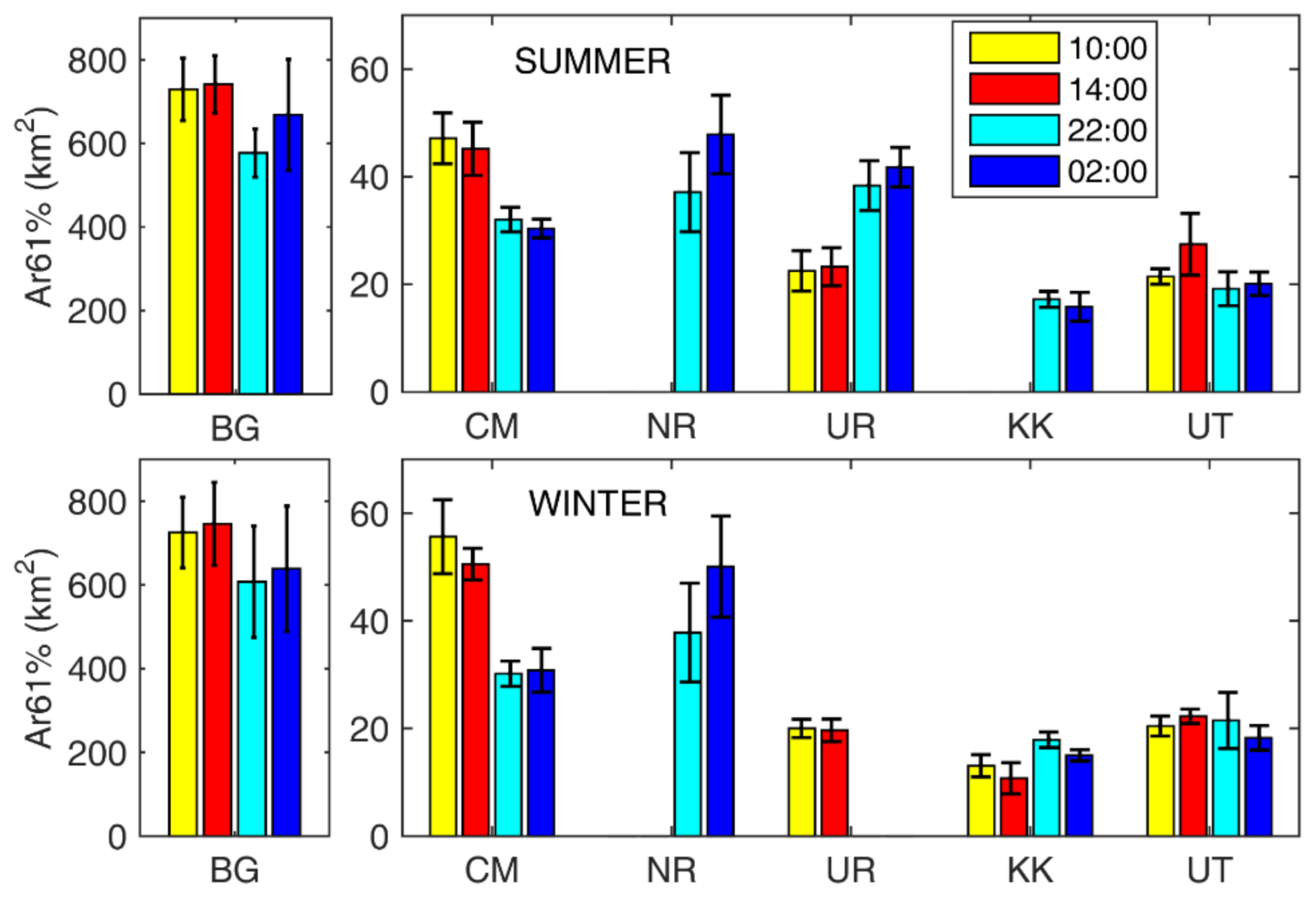
Figure 7 shows Ar61%. For BG and CM, the footprint area during daytime is greater than during nighttime, without significant seasonality differences. In addition, the two daytime values (10:00 and 14:00) are similar, as are the two nighttime ones (22:00 and 02:00). The std values suggest a moderate parameter variability across the years.
As pointed out previously, the parameters for NR daytime, KK summer daytime, and UR winter nighttime were not evaluated. As expected, the three smallest cities (UR, KK, and UT) exhibit smaller Ar61% footprints. The increased nighttime area of UR and KK reflects the behavior described in Section 4.1.
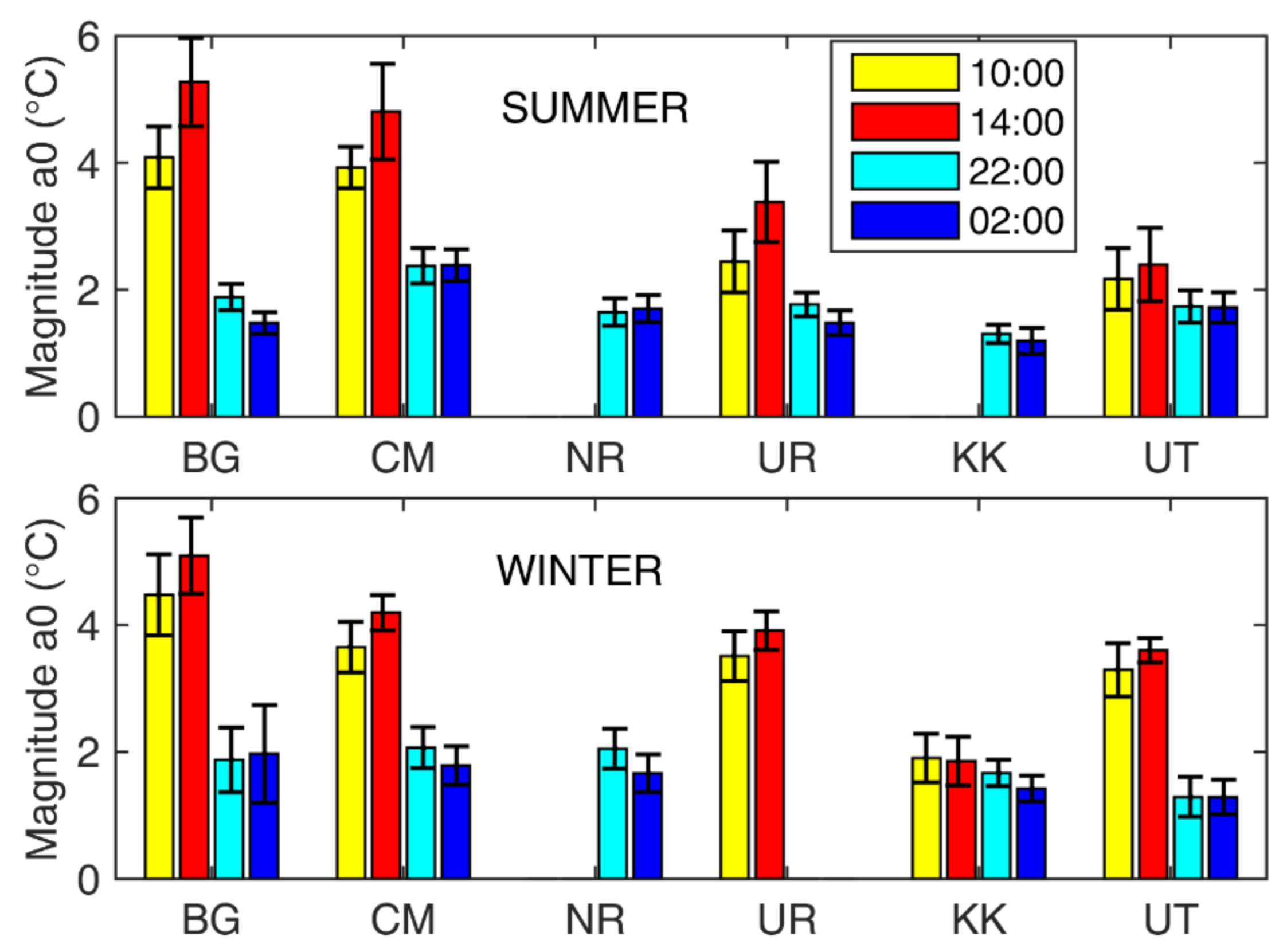
Figure 8 shows the mean magnitude a0 over the 14 years. All the cities demonstrate a cooling effect at nighttime. The SUHI magnitude during daytime is always higher than at night, again without seasonality differences. The nighttime mitigation of SUHI is evident for BG and CM. Indeed, as for UR and UT, the winter daytime a0 can be greater than the summer one. This is mainly ascribed to the winter cooling effect of the rural buffer, which exerts a consequent increasing of the SUHI (Equation (1)), even if the winter urban LST is lower than in summer.
The magnitude peak is reached at 14:00 in BG with 6.5 °C both in summer 2012 and in winter 2011. For all the cities, the a0 results at 14:00 confirm an interesting phenomenon discussed in [38]. Daytime SUHI magnitude generally increases as the background LST rises, showing an intensity peak at 14:00. When background LST increases from 10:00 to 14:00, the urban area absorbs more radiation compared to near rural areas, and urban LST experiences a faster increase than the rural surroundings. The a0 results also point out the different underlying mechanisms between day and night SUHI, as discussed later, considering that the background LST is more correlated to daytime SUHI compared to nighttime, as proved in [38].
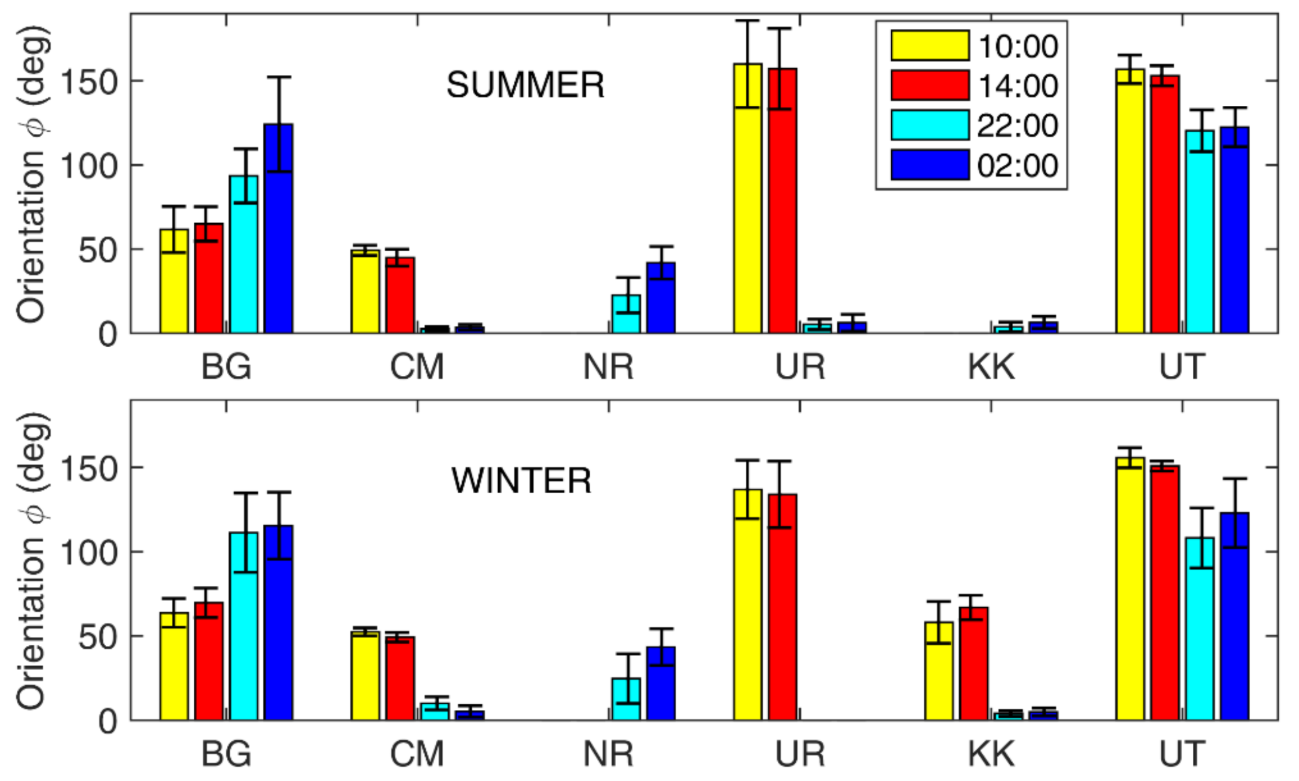
Mean and std of orientation angle φ are reported in Figure 9. This parameter depicts the layout of the Gaussian footprint in each map. The results highlight how the orientation keeps the same behavior for both the seasons, but exhibits differences between daytime and nighttime for some cities.
For instance, the daytime footprint orientation of BG is about 65° (i.e., along the NE–SW quarters) and follows the urban area constituted by residential and commercial zones, distinctly deployed in the NE–SW quarters [28,39]. These urban features, combined with the traffic congestion in the road network due to intense human activities, generate for BG the significant daytime SUHI pattern, both in summer and winter. During nighttime, the absence of solar forcing and the reduced working activities contribute to mitigation of the heating intensity and to modification of the SUHI footprint and orientation of BG, as also visible in BG panels of Figure 5.
The same behavior is found for CM, where the daytime direction of the SUHI footprint along the NE–SW quarters follows the layout of residential and commercial zones [40]. During the nighttime, there is a significant cooling effect of the urban core and outskirts, causing a reduction of Ar61%, a0, and a φ modification, as also noticeable in CM panels of Figure 5.
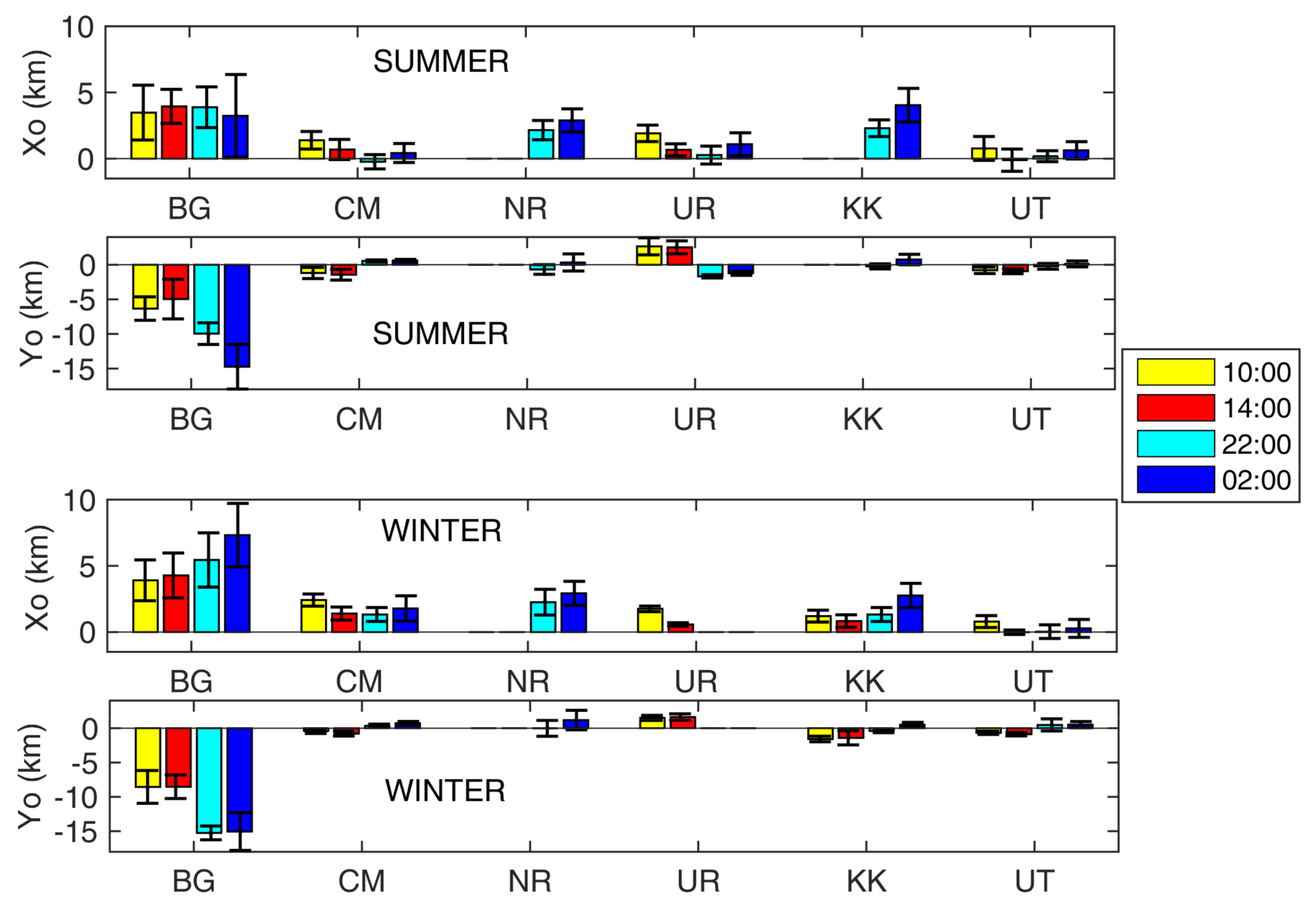
Figure 10 shows the central location (x0, y0) of the Gaussian surface expressed as distance from to the center of the map (0, 0); the map center roughly corresponds to the city center. Except for BG, whose urban extension is considerably wider than the other cities, the mean shift of the center of the Gaussian footprints (with respect to the map center) is small both seasonally and daily. For BG, (x0, y0) moves always towards southeast, with a displacement of the order of 5–10 km in daytime. This central location is positioned in the core of the high-density residential and commercial zone, also including government institutes and public utility zones [28,39]. At nighttime, the BG footprint shift is pronounced in the south direction, indicating the permanence of an urban heating towards the coastal zone. This fact could suggest a nocturnal sea influence, as discussed in [41].
4.3. Yearly Trend of SUHI Footprint and Magnitude
A comparative analysis of the footprint area Ar61% and magnitude a0 as a function of the 14-year interval (2003–2016) was performed to provide a specific-city and intercity overview of the SUHI trend. These parameters were compared with the urban area evolution across the years, computed from LULC Landsat maps (Figure 2) to analyze how the urban growth affects the SUHI pattern for both daytime and nighttime. Since previous results showed a weak seasonality dependence, Ar61% and a0 were averaged over summer and winter maps for each year.
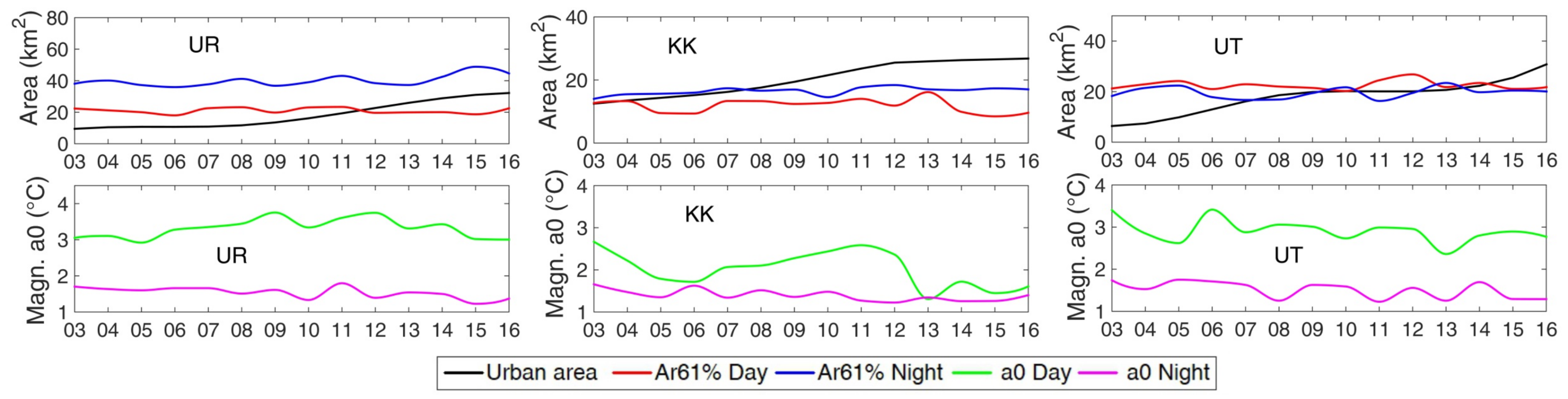
The upper panels of Figure 11 show the yearly trend of the urban area (black line) computed from LULC Landsat data inside the boundary map of Figure 3, compared with the daytime (red line) and nighttime (blue line) Ar61% for BG, CM, and NR. Lower panels report the daytime (green line) and nighttime (magenta line) a0 values. The curves were obtained as shape-preserving interpolants over the 14-year points. The same is reported in Figure 12 for UR, KK, and UT.
For each city, the urban growth during the years is either weakly correlated or not correlated with the SUHI footprint trend, whereas no correlation is found with the a0 trend. Particularly, daytime A61% values for BG slightly increases from 660 km2 to around 800 km2 between 2003 and 2016, exhibiting a correlation coefficient r = 0.9 with the urban area trend. Daytime A61% values for CM increase from 42 km2 to 54 km2, but with r = 0.6 with respect to the urban increase. Instead, nighttime A61% for BG, CM, and NR are unrelated to city growth. For the three smaller cities (i.e., UR, KK and UT), the urban expansion does not affect the daytime and nighttime SUHI footprint.
Figure 11 and Figure 12 show how the magnitude a0 is decorrelated with the city sprawl across the years. As expected, maximum SUHI intensities are mainly driven by specific yearly thermal conditions regardless of urban growth. These results confirm how the spatiotemporal urban heating patterns depend strongly on the background climate, such as precipitation, air temperature, solar radiation, and wind speed [18].
BG shows the highest annual a0 during daytime, with values ranging between 4 °C and 6 °C. During nighttime, a0 is rather similar for all the six cities, between 1 °C and 2 °C, even if CM shows mean values around 2.4 °C between 2003 and 2010.
The day–night magnitude difference may be ascribed to different factors, such as the different solar radiation absorption between urban and rural areas, since urban surfaces have a larger heat capacity and can absorb and store large amounts of thermal radiation with a higher rate than the rural surroundings [42]. Furthermore, anthropogenic heat released from energy consumption is an important contributor to urban warming and it is positively correlated with the urban heat island intensity [43,44]. Heat release from energy consumption (e.g., air conditioning systems, industrial heat generation, and energy use in transportation) usually increases during daytime due to intense human and economic activities [45]. The activities and transportation in larger urban areas, such as BG and CM, are expected to generate greater amounts of anthropogenic heat release, contributing to the rise of the daytime a0 values for BG and CM with respect to the smaller cities.
The lack of correlation for Ar61% and a0 with the urban sprawl over the years, except for the slight increase of BG and CM daytime footprints, can be ascribed to different mechanisms underlying the SUHI phenomenon [46]. A possible reason is linked to the outskirt sprawl. Considering the LULC Landsat maps and overlapping the different yearly scenes of Figure 2, it emerges that the new outskirt areas have a lower density of built-up pixels than the city core, especially for the small cities.
To better understand how the growth or modifications of a city affect the SUHI patterns, different factors at large and fine spatial scales should be considered. Some works found that urbanization warmed the LST on an annual mean scale, regardless of urban area size [47,48]. The size influence on SUHI depends on urban compactness: stretched or disperse cities are preferable for urban heat island mitigation [6]. Outskirts and suburban areas, if not densely urbanized, contain wide rural patches containing soil moisture, thus helping reduce the warming rate of the suburban zones [49]. Therefore, the results in Figure 11 and Figure 12 confirm the background climate influence on the heating trend over the years and suggest that the weak SUHI–urban growth relationship is ascribed to a lack of compactness in the urban sprawl, especially for the smaller cities investigated.
It is interesting to highlight other specific drivers of SUHI arising in the urban expansion and modification. Urbanization causes land cover changes, but the analysis of the urban heat island pattern should consider the heterogeneity of the new urban surfaces (materials and uses) and associated LST dynamics, as reported for Bangkok in [28]. Land cover changes from rural to urban affect the daytime and nighttime SUHI in different ways, depending on the rural category (grassland, cropland, shrub, forest) [50]. In the study cases, the rural surroundings exhibit a marked land cover variability with evident seasonal surface thermal changes.
Factors related to the urban texture at district level that affect the SUHI phenomenon—driving the heat trapping and absorption—rely on surface albedo, material, and color; on building layout, slope, and height; and on greenery cover [51,52,53,54]. At the same time, the urban texture can intensify the warming effect by reducing the wind circulation [55]. These factors suggest how the relationship SUHI–urban growth can show different trends and correlations, depending on the city specificity.
5. Conclusions
The SUHI pattern can be influenced by different factors, depending on external (location, climate) and intrinsic (city size and sprawl, land use, human activities) features. This work shows that the biggest cities, CM and BG, have higher daytime SUHI intensities, with pattern shape and layout related to the urban land use (e.g., high-density residential and commercial zones). At nighttime, SUHI intensities decrease for all cities and the heating pattern features generally change. This analysis highlights how the background climate and the intrinsic factors—such as human activities, transportation, and land use—contribute to the SUHI increase, especially at daytime and for the wider cities. Instead, the SUHI pattern is not correlated with the urban growth over the years: if the city sprawl is not compact and the new areas have low built-up density, the urban growth influence on SUHI is very weak.
The study of the SUHI temporal–spatial trend provides scientific support for urban land use policy to regulate and plan the intrinsic factors. For this purpose, the use of remote sensing data is unavoidable. Whereupon, suitable tools to process remote sensor data can be useful to perform quantitative analysis and comparisons of urban heating patterns, supplying indications that can be specific for a city but also can represent general signatures.
This study has also pointed out the usefulness of MODIS data for temporal sampling, but the low spatial resolution, suitable for Gaussian fitting, is a limit hindering SUHI investigation at district level. The possible options (Landsat and aircraft thermal images) have restricted or sporadic overpass times. These technical features motivate the future development of satellite constellations with the aim to improve, simultaneously, spatial and temporal resolutions.
Supplementary Materials
The following are available online at https://www.mdpi.com/2072-4292/10/5/665/s1, Figure S1: Yearly maps for BG, CM, NR, Figure S2: Yearly maps for UR, KK, UT.
Author Contributions
C.K. and S.B. conceived and designed the experiments; C.K. performed the experiments; C.K. and S.B. analyzed the data; S.B. wrote the paper.
Acknowledgments
We wish to thank Roberta Anniballe for the Gaussian fit tool development.
Conflicts of Interest
The authors declare no conflict of interest.
References
- Fallmann, J.; Forkel, R.; Emeis, S. Secondary Effects of Urban Heat Island Mitigation Measures on Air Quality. Atmos. Environ. 2016, 125, 199–211. [Google Scholar] [CrossRef]
- Bhargava, A.; Lakmini, S.; Bhargava, S. Urban Heat Island Effect: It’s Relevance in Urban Planning. J. Biodivers. Endanger. Spec. 2017, 5, 1–4. [Google Scholar] [CrossRef]
- De Ridder, K.; Maiheu, B.; Lauwaet, D.; Daglis, I.; Keramitsoglou, I.; Kourtidis, K.; Manunta, P.; Paganini, M. Urban Heat Island Intensification during Hot Spells—The Case of Paris during the Summer of 2003. Urban Sci. 2016, 1, 3. [Google Scholar] [CrossRef]
- Chen, W.; Zhang, Y.; Pengwang, C.; Gao, W. Evaluation of Urbanization Dynamics and Its Impacts on Surface Heat Islands: A Case Study of Beijing, China. Remote Sens. 2017, 9, 453. [Google Scholar] [CrossRef]
- Taha, H. Urban Climates and Heat Islands: Albedo, Evapotranspiration, and Anthropogenic Heat. Energy Build. 1997, 25, 99–103. [Google Scholar] [CrossRef]
- Zhou, B.; Rybski, D.; Kropp, J.P. The Role of City Size and Urban Form in the Surface Urban Heat Island. Sci. Rep. 2017, 7, 4791. [Google Scholar] [CrossRef] [PubMed]
- Oke, T.R. City Size and the Urban Heat Island. Atmos. Environ. 1973, 7, 769–779. [Google Scholar] [CrossRef]
- Santamouris, M. Analysing the heat island magnitude and characteristics in one hundred Asian and Australian cities and region. Sci. Total Environ. 2015, 512–513, 582–598. [Google Scholar] [CrossRef] [PubMed]
- Azevedo, J.; Chapman, L.; Muller, C. Quantifying the Daytime and Night-Time Urban Heat Island in Birmingham, UK: A Comparison of Satellite Derived Land Surface Temperature and High Resolution Air Temperature Observations. Remote Sens. 2016, 8, 153. [Google Scholar] [CrossRef]
- Anniballe, R.; Bonafoni, S.; Pichierri, M. Spatial and Temporal Trends of the Surface and Air Heat Island over Milan Using MODIS Data. Remote Sens. Environ. 2014, 150, 163–171. [Google Scholar] [CrossRef]
- Kourtidis, K.; Georgoulias, A.K.; Rapsomanikis, S.; Amiridis, V.; Keramitsoglou, I.; Hooyberghs, H.; Maiheu, B.; Melas, D. A Study of the Hourly Variability of the Urban Heat Island Effect in the Greater Athens Area during Summer. Sci. Total Environ. 2015, 517, 162–177. [Google Scholar] [CrossRef] [PubMed]
- Rasul, A.; Balzter, H.; Smith, C.; Remedios, J.; Adamu, B.; Sobrino, J.; Srivanit, M.; Weng, Q. A Review on Remote Sensing of Urban Heat and Cool Islands. Land 2017, 6, 38. [Google Scholar] [CrossRef]
- Rajasekar, U.; Weng, Q. Spatio-Temporal Modelling and Analysis of Urban Heat Islands by Using Landsat TM and ETM+ Imagery. Int. J. Remote Sens. 2009, 30, 3531–3548. [Google Scholar] [CrossRef]
- Fan, C.; Myint, S.W.; Kaplan, S.; Middel, A.; Zheng, B.; Rahman, A.; Huang, H.P.; Brazel, A.; Blumberg, D.G. Understanding the Impact of Urbanization on Surface Urban Heat Islands-A Longitudinal Analysis of the Oasis Effect in Subtropical Desert Cities. Remote Sens. 2017, 9, 672. [Google Scholar] [CrossRef]
- Haashemi, S.; Weng, Q.; Darvishi, A.; Alavipanah, S. Seasonal Variations of the Surface Urban Heat Island in a Semi-Arid City. Remote Sens. 2016, 8, 352. [Google Scholar] [CrossRef]
- Pichierri, M.; Bonafoni, S.; Biondi, R. Satellite Air Temperature Estimation for Monitoring the Canopy Layer Heat Island of Milan. Remote Sens. Environ. 2012, 127, 130–138. [Google Scholar] [CrossRef]
- Wang, K.; Wang, J.; Wang, P.; Sparrow, M.; Yang, J.; Chen, H. Influences of urbanization on surface characteristics as derived from the Moderate-Resolution Imaging Spectroradiometer: A case study for the Beijing metropolitan area. J. Geophys. Res. Atmos. 2007, 112, D22S06. [Google Scholar] [CrossRef]
- Zhou, D.; Bonafoni, S.; Zhang, L.; Wang, R. Remote sensing of the urban heat island effect in a highly populated urban agglomeration area in East China. Sci. Total Environ. 2018, 628–629, 415–429. [Google Scholar] [CrossRef] [PubMed]
- Deilami, K.; Kamruzzaman, M.; Hayes, J. Correlation or Causality between Land Cover Patterns and the Urban Heat Island Effect? Evidence from Brisbane, Australia. Remote Sens. 2016, 8, 716. [Google Scholar] [CrossRef]
- Onishi, A.; Cao, X.; Ito, T.; Shi, F.; Imura, H. Evaluating the Potential for Urban Heat-Island Mitigation by Greening Parking Lots. Urban For. Urban Green. 2010, 9, 323–332. [Google Scholar] [CrossRef]
- Alavipanah, S.; Wegmann, M.; Qureshi, S.; Weng, Q.; Koellner, T. The Role of Vegetation in Mitigating Urban Land Surface Temperatures: A Case Study of Munich, Germany during the Warm Season. Sustainability 2015, 7, 4689–4706. [Google Scholar] [CrossRef]
- Jongtanom, Y.; Kositanont, C.; Baulert, S. Temporal Variations of Urban Heat Island Intensity in Three Major Cities, Thailand. Mod. Appl. Sci. 2011, 5, 105–110. [Google Scholar] [CrossRef]
- Arifwidodo, S.D.; Tanaka, T. The Characteristics of Urban Heat Island in Bangkok, Thailand. Procedia Soc. Behav. Sci. 2015, 195, 423–428. [Google Scholar] [CrossRef]
- Arifwidodo, S.; Chandrasiri, O. Urban Heat Island and Household Energy Consumption in Bangkok, Thailand. Energy Proc. 2015, 79, 189–194. [Google Scholar] [CrossRef]
- Srivanit, M.; Hokao, K. Effects of Urban Development and Spatial Characteristics on Urban Thermal Environment in Chiang Mai Metropolitan, Thailand. Lowl. Technol. Int. 2012, 14, 9–22. [Google Scholar]
- Laosuwan, T.; Sangpradit, S. Urban Heat Island Monitoring and Analysis by Using Integration of Satellite Data and Knowledge Based Method. Int. J. Dev. Sustain. 2012, 1, 99–110. [Google Scholar]
- Tran, H.; Uchihama, D.; Ochi, S.; Yasuoka, Y. Assessment with satellite data of the urban heat island effects in Asian mega cities. Int. J. Appl. Earth Obs. Geoinf. 2006, 8, 34–48. [Google Scholar] [CrossRef]
- Keeratikasikorn, C.; Bonafoni, S. Urban Heat Island Analysis over the Land Use Zoning Plan of Bangkok by Means of Landsat 8 Imagery. Remote Sens. 2018, 10, 440. [Google Scholar] [CrossRef]
- Distributed Active Archive Center DAAC ORNL. Available online: https://daac.ornl.gov/get_data/ (accessed on 1 September 2017).
- US Geological Survey USGS. Available online: http://earthexplorer.usgs.gov (accessed on 12 December 2017).
- Bolstad, P.V.; Lillesand, T.M. Rapid Maximum Likelihood Classification. Photogramm. Eng. Remote Sens. 1991, 57, 67–74. [Google Scholar]
- Phiri, D.; Morgenroth, J. Developments in Landsat Land Cover Classification Methods: A Review. Remote Sens. 2017, 9, 967. [Google Scholar] [CrossRef]
- Congalton, R.G.; Green, K. Assessing the Accuracy of Remotely Sensed Data. Principles and Practices; Lewis Publishers: Boca Raton, FL, USA, 1999. [Google Scholar]
- Streutker, D. Satellite-Measured Growth of the Urban Heat Island of Houston, Texas. Remote Sens. Environ. 2003, 85, 282–289. [Google Scholar] [CrossRef]
- Anniballe, R.; Bonafoni, S. A Stable Gaussian Fitting Procedure for the Parameterization of Remote Sensed Thermal Images. Algorithms 2015, 8, 82–91. [Google Scholar] [CrossRef] [Green Version]
- Quan, J.; Chen, Y.; Zhan, W.; Wang, J.; Voogt, J.; Wang, M. Multi-temporal trajectory of the urban heat island centroid in Beijing, China based on a Gaussian volume model. Remote Sens. Environ. 2014, 149, 33–46. [Google Scholar] [CrossRef]
- Zhou, J.; Chen, Y.H.; Li, J.; Weng, Q.H.; Yi, W.B. A volume model for urban heat island based on remote sensing imagery and its application: A case study in Beijing. Int. J. Remote Sens. 2008, 12, 734–742. [Google Scholar]
- Zhao, G.; Dong, J.; Liu, J.; Zhai, J.; Cui, Y.; He, T.; Xiao, X. Different Patterns in Daytime and Nighttime Thermal Effects of Urbanization in Beijing-Tianjin-Hebei Urban Agglomeration. Remote Sens. 2017, 9, 121. [Google Scholar] [CrossRef]
- Department of Public Works and Town & Country Planning. Available online: https://dpt.go.th/en/ (accessed on 5 February 2018).
- McGrath, B.; Sangawongse, S.; Thaikatoo, D.; Corte, M.B. The Architecture of the Metacity: Land Use Change, Patch Dynamics and Urban Form in Chiang Mai, Thailand. Urban Plan. 2017, 2, 53. [Google Scholar] [CrossRef]
- Stathopoulou, M.; Cartalis, C.; Keramitsoglou, I. Mapping Micro-Urban Heat Islands Using NOAA/AVHRR Images and CORINE Land Cover: An Application to Coastal Cities of Greece. Int. J. Remote Sens. 2004, 25, 2301–2316. [Google Scholar] [CrossRef]
- Jin, M.S.; Kessomkiat, W.; Pereira, G. Satellite-Observed Urbanization Characters in Shanghai, China: Aerosols, Urban Heat Island Effect, and Land–Atmosphere Interactions. Remote Sens. 2011, 3, 83–99. [Google Scholar] [CrossRef]
- Du, H.; Wang, D.; Wang, Y.; Zhao, X.; Qin, F.; Jiang, H.; Cai, Y. Influences of land cover types, meteorological conditions, anthropogenic heat and urban area on surface urban heat island in the Yangtze River Delta Urban Agglomeration. Sci. Total Environ. 2016, 571, 461. [Google Scholar] [CrossRef] [PubMed]
- Liao, W.; Liu, X.; Wang, D.; Sheng, Y. The Impact of Energy Consumption on the Surface Urban Heat Island in China’s 32 Major Cities. Remote Sens. 2017, 9, 250. [Google Scholar] [CrossRef]
- Shahmohamadi, P.; Che-Ani, A.I.; Etessam, I.; Maulud, K.N.A.; Tawil, N.M. Healthy Environment: The Need to Mitigate Urban Heat Island Effects on Human Health. Procedia Eng. 2011, 20, 61–70. [Google Scholar] [CrossRef]
- Arnds, D.; Böhner, J.; Bechtel, B. Spatio-temporal variance and meteorological drivers of the urban heat island in a European city. Theor. Appl. Climatol. 2017, 128, 43–61. [Google Scholar] [CrossRef]
- Peng, S.; Piao, S.; Ciais, P.; Friedlingstein, P.; Ottle, C.; Bréon, F.M.; Nan, H.; Zhou, L.; Myneni, R.B. Surface urban heat island across 419 global big cities. Environ. Sci. Technol. 2012, 46, 696–703. [Google Scholar] [CrossRef] [PubMed]
- Zhou, D.; Zhao, S.; Liu, S.; Zhang, L.; Zhu, C. Surface urban heat island in China’s 32 major cities: Spatial patterns and drivers. Remote Sens. Environ. 2014, 152, 51–61. [Google Scholar] [CrossRef]
- Zhou, D.; Li, D.; Sun, G.; Zhang, L.; Liu, Y.; Hao, L. Contrasting effects of urbanization and agriculture on surface temperature in eastern China. J. Geophys. Res. Atmos. 2016, 121, 9597–9606. [Google Scholar] [CrossRef]
- MacLachlan, A.; Biggs, E.; Roberts, G.; Boruff, B. Urbanisation-Induced Land Cover Temperature Dynamics for Sustainable Future Urban Heat Island Mitigation. Urban Sci. 2017, 1, 38. [Google Scholar] [CrossRef]
- Zhao, Q.; Myint, S.W.; Wentz, E.A.; Fan, C. Rooftop Surface Temperature Analysis in an Urban Residential Environment. Remote Sens. 2015, 7, 12135–12159. [Google Scholar] [CrossRef]
- Bonafoni, S.; Baldinelli, G.; Verducci, P. Sustainable strategies for smart cities: Analysis of the town development effect on surface urban heat island through remote sensing methodologies. Sustain. Cities Soc. 2017, 29, 211–218. [Google Scholar] [CrossRef]
- Zhang, H.; Jing, X.-M.; Chen, J.-Y.; Li, J.-J.; Schwegler, B. Characterizing Urban Fabric Properties and Their Thermal Effect Using QuickBird Image and Landsat 8 Thermal Infrared (TIR) Data: The Case of Downtown Shanghai, China. Remote Sens. 2016, 8, 541. [Google Scholar] [CrossRef]
- Bonafoni, S.; Baldinelli, G.; Verducci, P.; Presciutti, A. Remote Sensing Techniques for Urban Heating Analysis: A Case Study of Sustainable Construction at District Level. Sustainability 2017, 9, 1308. [Google Scholar] [CrossRef]
- Li, D.; Bou-Zeid, E. Synergistic interactions between urban heat islands and heat waves: The impact in cities is larger than the sum of its parts. J. Appl. Meteorol. Climatol. 2013, 52, 2051–2064. [Google Scholar] [CrossRef]
Figure 1.
Location of the analyzed six cities on a Thailand administrative boundary map.

Figure 2.
Maps of urban surface (red) evolution for the six cities in the years 2004, 2008, 2012, and 2016 obtained from Landsat data (see Section 3.1). From top: Bangkok (BG), Chiang Mai (CM), Nakhon Ratchasima (NR), Ubon Ratchathani (UR), Khon Kaen (KK), and Udon Thani (UT). All panels represent a 30 × 30 km area except for Bangkok, 90 × 90 km.

Figure 3.
Urban and rural category maps from MODIS MCD12Q1 product of 2013 for the six cities (1 km pixel size) used for the computation of the reference rural land surface temperature (LSTRUR) (rural buffer).
Figure 3.
Urban and rural category maps from MODIS MCD12Q1 product of 2013 for the six cities (1 km pixel size) used for the computation of the reference rural land surface temperature (LSTRUR) (rural buffer).

Figure 4.
Surface urban heat island (SUHI) during summer 2013 for the six cities at 22:00.

Figure 5.
SUHI (°C) and Gaussian fitting during 2014 for Bangkok (BG), Chiang Mai (CM), and Nakhon Ratchasima (NR) for summer and winter, considering the diurnal variation at 10:00, 14:00, 22:00, and 02:00.
Figure 5.
SUHI (°C) and Gaussian fitting during 2014 for Bangkok (BG), Chiang Mai (CM), and Nakhon Ratchasima (NR) for summer and winter, considering the diurnal variation at 10:00, 14:00, 22:00, and 02:00.

Figure 6.
SUHI (°C) and Gaussian fitting during 2014 for Ubon Ratchathani (UR), Khon Kaen (KK), and Udon Thani (UT) for summer and winter, considering the diurnal variation at 10:00, 14:00, 22:00, and 02:00.
Figure 6.
SUHI (°C) and Gaussian fitting during 2014 for Ubon Ratchathani (UR), Khon Kaen (KK), and Udon Thani (UT) for summer and winter, considering the diurnal variation at 10:00, 14:00, 22:00, and 02:00.

Figure 7.
Intercity comparison of Gaussian footprint area Ar61% (km2) during summer (upper panel) and winter (bottom panel). Ar61% is averaged over the 14 years, considering the diurnal variation at 10:00, 14:00, 22:00, and 02:00. The black bar is the standard deviation across the years.
Figure 7.
Intercity comparison of Gaussian footprint area Ar61% (km2) during summer (upper panel) and winter (bottom panel). Ar61% is averaged over the 14 years, considering the diurnal variation at 10:00, 14:00, 22:00, and 02:00. The black bar is the standard deviation across the years.

Figure 8.
Intercity comparison of Gaussian magnitude a0 (°C) during summer (upper panel) and winter (bottom panel); a0 is averaged over the 14 years, considering the diurnal variation at 10:00, 14:00, 22:00, and 02:00. The black bar is the standard deviation across the years.
Figure 8.
Intercity comparison of Gaussian magnitude a0 (°C) during summer (upper panel) and winter (bottom panel); a0 is averaged over the 14 years, considering the diurnal variation at 10:00, 14:00, 22:00, and 02:00. The black bar is the standard deviation across the years.

Figure 9.
Intercity comparison of orientation angle φ (degree) during summer (upper panel) and winter (bottom panel); φ is averaged over the 14 years, considering the diurnal variation at 10:00, 14:00, 22:00, and 02:00. The black bar is the standard deviation across the years.
Figure 9.
Intercity comparison of orientation angle φ (degree) during summer (upper panel) and winter (bottom panel); φ is averaged over the 14 years, considering the diurnal variation at 10:00, 14:00, 22:00, and 02:00. The black bar is the standard deviation across the years.

Figure 10.
Intercity comparison of central location (x0, y0) (km) during summer (upper panels) and winter (bottom panels). Central location is averaged over the 14 years, considering the diurnal variation at 10:00, 14:00, 22:00, and 02:00. The black bar is the standard deviation across the years.
Figure 10.
Intercity comparison of central location (x0, y0) (km) during summer (upper panels) and winter (bottom panels). Central location is averaged over the 14 years, considering the diurnal variation at 10:00, 14:00, 22:00, and 02:00. The black bar is the standard deviation across the years.

Figure 11.
BG, CM, and NR: yearly trend (2003–2016) of the urban area computed from land use and land cover (LULC) Landsat maps (black line, upper panel), daytime Ar61% (red line, upper panel), nighttime Ar61% (blue line, upper panel), daytime a0 (green line, lower panel), and nighttime a0 (magenta line, lower panel). For NR, daytime a0 is the maximum SUHI value, since daytime Gaussian fitting is not reliable.

Figure 12.
UR, KK, and UT yearly trend (2003–2016) of the urban area computed from LULC Landsat maps (black line, upper panel), daytime Ar61% (red line, upper panel), nighttime Ar61% (blue line, upper panel), daytime a0 (green line, lower panel), and nighttime a0 (magenta line, lower panel).
Figure 12.
UR, KK, and UT yearly trend (2003–2016) of the urban area computed from LULC Landsat maps (black line, upper panel), daytime Ar61% (red line, upper panel), nighttime Ar61% (blue line, upper panel), daytime a0 (green line, lower panel), and nighttime a0 (magenta line, lower panel).


Table 1.
Correlation coefficient r between SUHI from MODIS (MODerate Resolution Imaging Spectroradiometer) and Gaussian surface for the six cities. The mean r value over the years 2003–2016 is reported in brackets. x = reliable Gaussian fit; - = no Gaussian fit.
Table 1.
Correlation coefficient r between SUHI from MODIS (MODerate Resolution Imaging Spectroradiometer) and Gaussian surface for the six cities. The mean r value over the years 2003–2016 is reported in brackets. x = reliable Gaussian fit; - = no Gaussian fit.
| City | Season | 10:00 | 14:00 | 22:00 | 02:00 |
|---|---|---|---|---|---|
| Bangkok | Summer | x (0.70) | x (0.70) | x (0.75) | x (0.75) |
| Winter | x (0.74) | x (0.73) | x (0.66) | x (0.64) | |
| Chiang May | Summer | x (0.73) | x (0.73) | x (0.90) | x (0.87) |
| Winter | x (0.71) | x (0.69) | x (0.86) | x (0.82) | |
| Nakhon | Summer | - | - | x (0.72) | x (0.82) |
| Ratchasima | Winter | - | - | x (0.73) | x (0.79) |
| Ubon | Summer | x (0.60) | x (0.63) | x (0.87) | x (0.83) |
| Ratchathani | Winter | x (0.73) | x (0.69) | - | - |
| Khon Kaen | Summer | - | - | x (0.81) | x (0.77) |
| Winter | x (0.73) | x (0.68) | x (0.82) | x (0.82) | |
| Udon Thani | Summer | x (0.71) | x (0.70) | x (0.81) | x (0.84) |
| Winter | x (0.88) | x (0.88) | x (0.67) | x (0.70) |
© 2018 by the authors. Licensee MDPI, Basel, Switzerland. This article is an open access article distributed under the terms and conditions of the Creative Commons Attribution (CC BY) license (http://creativecommons.org/licenses/by/4.0/).
Share and Cite
MDPI and ACS Style
Keeratikasikorn, C.; Bonafoni, S. Satellite Images and Gaussian Parameterization for an Extensive Analysis of Urban Heat Islands in Thailand. Remote Sens. 2018, 10, 665. https://doi.org/10.3390/rs10050665
AMA Style
Keeratikasikorn C, Bonafoni S. Satellite Images and Gaussian Parameterization for an Extensive Analysis of Urban Heat Islands in Thailand. Remote Sensing. 2018; 10(5):665. https://doi.org/10.3390/rs10050665
Chicago/Turabian StyleKeeratikasikorn, Chaiyapon, and Stefania Bonafoni. 2018. "Satellite Images and Gaussian Parameterization for an Extensive Analysis of Urban Heat Islands in Thailand" Remote Sensing 10, no. 5: 665. https://doi.org/10.3390/rs10050665
Note that from the first issue of 2016, this journal uses article numbers instead of page numbers. See further details here.