Impact of Cycle Time and Payload of an Industrial Robot on Resource Efficiency
by
 , , , and
Florian Stuhlenmiller
1,* ,
,
Steffi Weyand
2,
Jens Jungblut
1,
Liselotte Schebek
2,
Debora Clever
1 and
Stephan Rinderknecht
1 
1
Institute for Mechatronic Systems in Mechanical Engineering, Technical University of Darmstadt, 64287 Darmstadt, Germany
2
Institute IWAR, Chair of Material Flow Management and Resource Economy, Technical University of Darmstadt, 64287 Darmstadt, Germany
*
Author to whom correspondence should be addressed.
Robotics 2021, 10(1), 33; https://doi.org/10.3390/robotics10010033
Submission received: 22 December 2020
/
Revised: 27 January 2021
/
Accepted: 8 February 2021
/
Published: 12 February 2021
(This article belongs to the Special Issue Industrial Robotics in Industry 4.0)
Abstract
:Modern industry benefits from the automation capabilities and flexibility of robots. Consequently, the performance depends on the individual task, robot and trajectory, while application periods of several years lead to a significant impact of the use phase on the resource efficiency. In this work, simulation models predicting a robot’s energy consumption are extended by an estimation of the reliability, enabling the consideration of maintenance to enhance the assessment of the application’s life cycle costs. Furthermore, a life cycle assessment yields the greenhouse gas emissions for the individual application. Potential benefits of the combination of motion simulation and cost analysis are highlighted by the application to an exemplary system. For the selected application, the consumed energy has a distinct impact on greenhouse gas emissions, while acquisition costs govern life cycle costs. Low cycle times result in reduced costs per workpiece, however, for short cycle times and higher payloads, the probability of required spare parts distinctly increases for two critical robotic joints. Hence, the analysis of energy consumption and reliability, in combination with maintenance, life cycle costing and life cycle assessment, can provide additional information to improve the resource efficiency.
1. Introduction
Rising energy prices and environmental awareness emphasize the importance of resource efficiency for the manufacturing industry. Energy efficiency is a key success factor for the reduction of operational resource consumption, both tangible such as corresponding emissions and intangible such as costs, and is therefore a target of the Industry 4.0 initiative [1,2]. In this context, methods and optimization strategies aimed at the reduction of energy consumed by industrial robots are for example investigated in [3,4,5,6]. Corresponding approaches propose the utilization of more efficient components and the integration of energy storage mechanisms, enabling recuperation on the hardware level of the industrial robot. Software approaches are manifold and include trajectory optimization for single robots as well as operation scheduling which considers sequencing and synchronization of different operations for a robotic cell or assembly line. The approaches are usually based on a detailed model of the industrial robot and the corresponding actuators. Usually, the energy efficiency is focused on the use phase, since the highest greenhouse gas emissions occur in this phase [3,7,8]. However, to draw a full picture of the resource efficiency, the full life cycle, including robot manufacturing, operation with actual tasks and robot motion, maintenance and end of life, has to be considered. Only two relevant studies take the full life cycle of robot system into account using the method of life cycle assessment (LCA) [7,8]. However, the actual task and motion of the industrial robots is not considered in detail. In addition, the service life and reliability of components are not part of these studies, even though they may influence life cycle impacts. For example, an optimization of the robot position and the motion pattern performed in [9,10] resulted in a distinctly reduced gear wear and increased service life, respectively. Correspondingly, a combined analysis fo energy consumption and service life indicated a conflict of interest between energy efficiency and lifetime depending on task and trajectory [11]. Similarly, an estimation of follow-up costs in [12] implies that approximately 60% results from consumed energy, while maintenance costs amount to 25%. In contrast, required spare parts account for 16.3% of the follow-up costs while expenses for energy are specified with 9.8% in [13]. Consequently, it can be expected that the specific task and motion may impact the production planning process and the resulting resource efficiency as well.
Therefore, we propose a comprehensive assessment of the resource efficiency, taking into account the energy consumption and the reliability of components in dependence of the robot’s trajectory. Considering maintenance activities and integrating the estimation of life cycle costs (LCC) as well as greenhouse gas (GHG) emissions allows one to evaluate the impact on resource efficiency. The contributions of this paper are summarized as follows:
- The dynamic model of a robot is extended to allow for the estimation of energy consumption and the prediction of the reliability of selected components for a given trajectory.
- Corresponding simulation results are used to identify critical components and the consideration of maintenance methods facilitates the estimation of required spare parts.
- Life cycle assessment and the life cycle costing are combined with the motion simulation to determine LCC and GHG emissions.
- The application to an exemplary robot, task and trajectory highlights the determination of critical components while a parametric study yields the impact of payload and cycle time on LCC and GHG emissions and demonstrates corresponding benefits for the decision-making.
The remainder of this paper is organized as follows: A model-based simulation of a robotic system is introduced in Section 2. The dynamic model of the robot is extended by an estimation of the consumed energy as well as a prediction of the lifetime of the gear units. The integration of maintenance, life cycle costing and LCA completes the proposed method and allows the estimation of the resource efficiency. The proposed method is applied to and analyzed for an exemplary task and system in Section 3. In addition, a parametric study is performed and the influence of payload and cycle time on costs and GHG emissions is investigated. Finally, Section 4 concludes the paper and proposes future research topics.
2. Extending a Motion Simulation with Cost Estimation and Emission Prediction
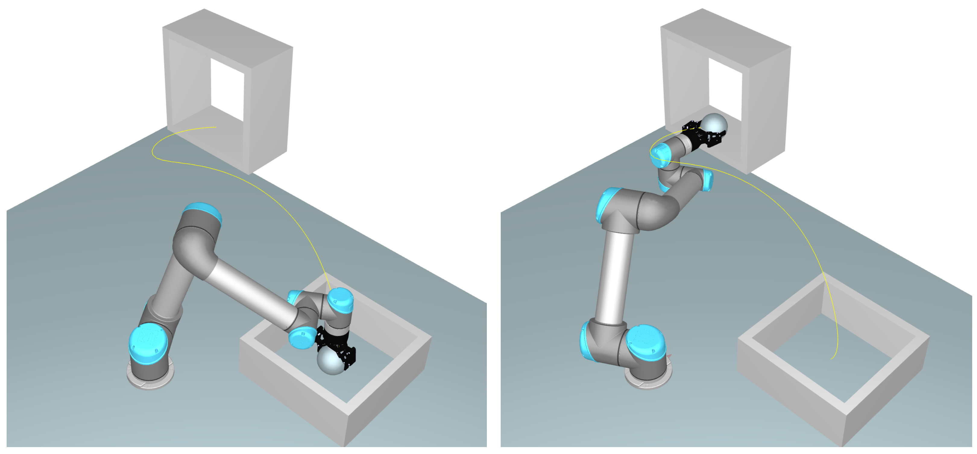
The aim of this work is the prediction of LCC and GHG emissions for a selected robot, task and trajectory. In the following, this will be presented for an exemplary robot performing a pick-and-place operation. Thereby, a workpiece is transported from one box to another as depicted in Figure 1 and the task can be characterized by the payload, the duration and the planned motion. The exemplary robot UR5 (Universal Robots A/S, Odense S, Denmark) is selected to perform the task. In order to estimate the LCC and perform the LCA based on a simulation of the robot’s motion, the consumed resources during the operation have to be determined. The selected task requires a robot, which has to be produced by the manufacturer and acquired by the user. While the task is performed, energy is consumed and damage accumulates in components of the robot. As a result, maintenance and spare parts may be required. Corresponding energy and maintenance costs are derived from models as described in the following.
2.1. Robot Modeling
The energy consumption of an industrial robot can be modeled based on the system dynamics, while considering mechanical and electrical characteristics of the actuators. The system dynamics are represented by the equations of motion which can be expressed according to:
where is the vector of joint coordinates, describes the inertia matrix, considers coriolis and centripetal torques, while includes gravitational loads. The robot is driven by the torque vector , while additional external forces or torques are not considered in this paper. Mechanical losses in the joints are considered by the friction torque . The equations of motion can be evaluated by the recursive Newton–Euler algorithm based on mechanical parameters. Corresponding kinematic and mass properties are provided by the robot manufacturer and are summarized in Table A1. Different payloads are additionally implemented as a point mass at the position with respect to the flange of the robot. Thus, the adapted mass and center of gravity of link 6 are determined according to:
The characteristics of the joint actuators can be considered based on the components utilized in the robot. The reducers used in the UR5 are strain wave gears and belong to the HFUS-2SH (Harmonic Drive AG, Limburg an der Lahn, Germany) family [14]. Based on the diameter of the robot joints, the size of the reducer can be estimated and the corresponding parameters used in this work are summarized in Table A2. To the best of the authors’ knowledge, detailed information about the motors is not publicly available. Thus, alternative motors that can be integrated with the reducers are selected to parameterize the electro-mechanical model of the motor. Furthermore, the rotational inertia includes the inertia of corresponding motor brakes. The corresponding parameters are listed in Table A3.
2.2. Energy Consumption Estimation
One relevant mechanical characteristic of the actuators related to the system dynamics is the reduced inertia, which is included in . It is assumed that the weight of the actuators is included in the weights of the links provided by the manufacturer, thus, the reduced rotational inertia has to be considered additionally. Furthermore, mechanical losses are considered in the drive train. A simple model describing the corresponding joint friction considers Coulomb and viscous friction with the coefficients and , respectively, and is given by [15]:
While more complex friction models, e.g., presented in [16,17], consider possible nonlinear and time-dependent effects such as load-dependency, more complex models are difficult to parameterize without an experimental evaluation. For the Coulomb and viscous friction model, the corresponding parameters are estimated based on the no-load running torque of the reducers as specified in the datasheet of the manufacturer [18] and the result is summarized in Table A4.
Modeling the electrical characteristics of the actuators allows one to determine the electrical energy consumption. Robotic joints are thereby often driven by geared brushless direct-current (DC) motors or geared permanent magnet synchronous machines. High torque requirements result in large reduction ratios , thus the motors are usually operated without field weakening. Hence, a simplified lumped parametric model of a DC motor can be utilized to describe the motor characteristics. Accordingly, the motor current I can be calculated from the corresponding joint torque to
where is the torque constant. Based on the terminal resistance R, inductance L and speed constant , the resulting motor voltage U can be calculated by the following equation:
Assuming that the utilized drive system does not allow recuperation, the electrical energy consumed during one cycle with the duration can be determined by integration of the electric power for each joint. The consumption of a serial manipulator with i joints as a whole is the sum of the n individual motors’ consumption. In addition, power required to keep the motor safety brakes open, as well as power consumed by peripherals and the controller, is considered by a constant consumption [19,20] and yields the following equation to calculate the energy consumption of the system:
2.3. Lifetime Modeling and Reliability Estimation
The lifetime of a robot is often related to the reducers in each joint as critical components [21,22,23]. Corresponding failure mechanisms can be manifold and may depend on several characteristics, such as topology, tooth geometry and environmental conditions. In the UR5, strain wave gears are utilized and the corresponding mean operating life , which represents the operating time corresponding to 50% reliability, of a single strain wave gear is determined in [18,23], based on the average life of the wave generator bearing. The mean life expectancy is calculated based on the rated service life , which is provided by the manufacturer for a rated speed , a rated torque and the actual load T, according to:
The corresponding load T is determined by:
Thereby, c describes the exponential relation of the stress-life curve for corresponding endurance curves [23]. According to information of the manufacturer [18], the rated torque and the torque are specified with respect to the output of the reducer. Thus, the equations of motion in Equation (1) are adapted, so that the friction torque and the rotor inertia of the motors do not impact the load. Accordingly, is calculated by:
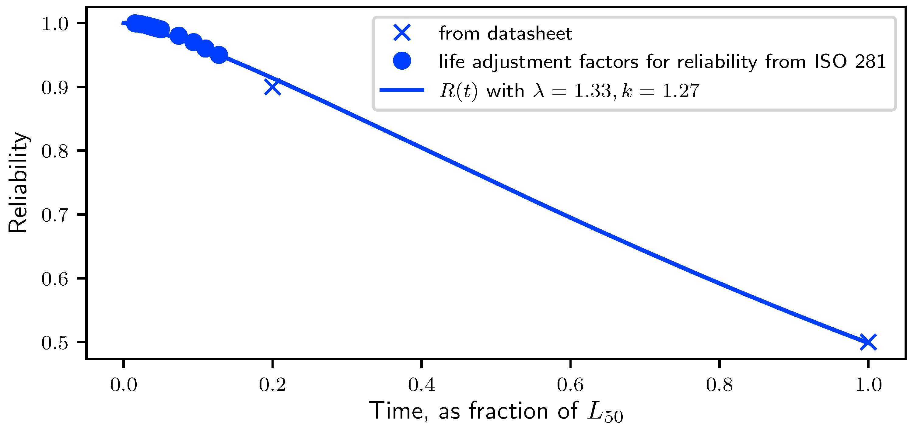
Instead of the lifetime, various maintenance approaches are based on the reliability of components or a system [24,25]. Ideally, the reliability is determined from lifetime tests, which are often time consuming and expensive. Lifetime tests of strain wave gears are presented for example in [26,27,28], however, these are focused on space applications and the evaluation of characteristics in vacuum and therefore differ from the investigated application and actual reducers used in the UR5. As the service life of strain wave gears is based on the wave generator bearing according to the manufacturer [18], the life adjustment factors for reliability for bearings given in ISO 281 [29] are used in the following to estimate the reliability of the reducers in the UR5. Therefore, the life adjustment factors are used to scale the life expectancy to determine operating times with lower failure probabilities. Furthermore, the manufacturer states that . Thus, a curve fit for the reliability depending on the operating time t can be performed based on a suitable cumulative distribution. Based on the available data, a two parametric Weibull distribution was selected, which is defined according to:
and is described by the scale parameter , as well as the shape parameter k [24]. The utilized data and the resulting fit are presented in Figure 2 and yield and .
Combining Equations (7) and (8) with Equation (10) links the reliability of the reducer with the actual trajectory and operating time and yields the following expression:
Based on the reliability of individual components , the system’s reliability can be determined based on its configuration. As the UR5 is a serial manipulator, the reliability of series configurations can be expressed by [24]:
Note that only considering the reducers for the system’s reliability as components is a simplification which can be used for the comparison of different trajectories.
2.4. Application of Maintenance Methods
Based on the reliability of each reducer calculated with Equation (11), maintenance strategies can be determined and evaluated for a specific trajectory instead of using characteristics such as a general mean time between failures. Several policies with different complexities exist in literature, e.g., age-dependent, periodic or condition-based. The evaluation can, for example, be performed analytically, with the Markov method or with the the Monte Carlo method [24,25]. As the focus of this paper is on highlighting the potential of combining the simulation of trajectories with procedures calculating the environmental impact and the economic costs, only corrective maintenance is selected to be performed during a planned, maximum operating duration as an example in the following. Thereby, the modular joint of the UR5 is completely replaced as soon as an error occurs. This results in a perfect repair of the joint but an imperfect repair of the system [25]. Furthermore, assuming that replacement parts are in storage and the duration of the repair is negligible compared to the operating duration, the availability of the system is simplified to be always 100%. More complex methods and strategies for optimal maintenance can, for example, be found in [25].
A Monte Carlo simulation is performed to determine the number of replacements for each joint due to its simple implementation for available probability distributions. The corresponding procedure, adapted from [25], is:
- (a)
- for a given trajectory, evaluate for each joint i from Equation (11) and determine the corresponding probability distribution function
- (b)
- based on this, draw random failure times for each joint i, until and collect the number of draws
- (c)
- repeat (b) for all samples
For all samples, the number of draws for each joint yields the probability of the number of required repairs and allows further consideration in the LCC and LCA.
2.5. Life Cycle Costing
Following the procedure of [12], acquisition costs, as well as follow up costs arising from energy consumption and maintenance, are considered. Thus, based on the consumed energy calculated with Equation (6) and the number of repairs , the costs arising during can be calculated for each sample of the Monte Carlo simulation according to:
with the acquisition costs , the electricity price and the maintenance costs by means of spare parts for the individual joints . As the impact of cycle time and payload of the robot is the focus of this work, only directly related costs are considered in this study, e.g., wages for operators, transport or disposal are not included. However, the cost estimation can be extended and adapted to individual production processes and use cases if the costs are known.
2.6. Life Cycle Assessment
Life cycle assessment, a method standardized by ISO 14040/14044 [30,31], is used to assess the GHG emissions over the life cycle of the exemplary robot system. The goal of the LCA is the investigation of the GHG emissions of different trajectories during the operation phase towards the emissions of the robot system. The scope of the LCA encompasses the manipulator and the controller. For a pick-and-place operation, the workpiece is considered by the impact on energy consumption and reliability. The functional unit as reference unit is defined as one robot system continuously operated for . Accordingly, the modeled life cycle of the robot system, the so-called product system in LCA, includes the following phases: (1) production phase of the controller and the robot including the emissions of the supply chain of the included materials and the simplified manufacturing of the robot’s components (2) the operation phase including the actual tasks and motion of the robot and (3) various maintenance actions and spare parts necessary during . Analogous to the estimation of LCC, the GHG emissions can be calculated for each sample according to:
with the emissions during the production phase and the emission factor for the electricity mix considering the impact of energy consumed during the operation of the robot. The manufacturing of additional spare parts required for corrective maintenance is represented by . The disposal phase is disregarded for two reasons. First, the GHG emissions are expected to be negligible compared to the rest of the life cycle; second, a detailed recycling process of the robot system is not known so far.
3. Exemplary Application and Potentials of the Method
In this section, the presented models are used to estimate the LCC and GHG emissions for an exemplary pick-and-place operation as depicted in Figure 1. The task itself can be partitioned into two phases: the first phase consists of picking up the workpiece at the initial position and transporting it to the final position . Two intermediate locations, and , are defined to avoid collisions with the obstacles. The second phase utilizes the same points in reverse. The location, orientation and configuration of the selected points for the task are given in Table 1. Both phases are defined to have the same duration and take into account 1 s per phase for opening or closing the tool, while the robot holds the corresponding position. Thus, the duration of the motion in each phase can be derived from the total duration of one cycle . For the multi-point trajectory, the duration of the motion is partitioned proportional to the maximum distance traveled in joint space into three individual intervals. A trajectory is generated in joint space via a piecewise spline of 5th degree to plan the motions of the robot, yielding smooth acceleration and velocity profiles. Angular acceleration and velocity are set to be zero at the start and end of the individual motions, respectively.
As the workpiece is placed at , the payload in the first phase consists of the gripper and the workpiece, while only the weight of the gripper is considered as the payload during the second phase. Thus, the dynamic model of the robot is updated between the two phases. Therefore, the exemplary gripper 2F-85 (Robotiq Inc., Lévis, QC, Canada) is applied with an approximated weight of 1 , while the center of mass is located at a distance of in z-direction with respect to the flange coordinate system. The center of gravity of the workpiece is assumed to be shifted an additional in z-direction. By adapting Equation (2), the corresponding mass and center of gravity of the payload can be calculated from the mass and center of gravity of tool and workpiece. The simulation software RoboDK (RoboDK Inc., Montreal, QC, Canada) is used to implement the task, determine the inverse kinematics and visualize the motion. The system dynamics are evaluated using a recursive Newton–Euler algorithm to directly provide the motor torque and the torque related to the useful life of the reducers .
For the evaluation, it is assumed that the robot perfectly follows the planned trajectory, and potentially occurring oscillations or vibrations are negligible. In addition, the degradation of the robot’s components during the useful life is assumed to not impact the performance, i.e., the energy consumed during one cycle remains constant. Furthermore, it is assumed that the effect of the environment, e.g., temperature or dust, as well as the consequence of events such as collisions or emergency stops during the operation, is not considered.
3.1. Estimation of Life Cycle Costs and Greenhouse Gas Emissions for Individual Components
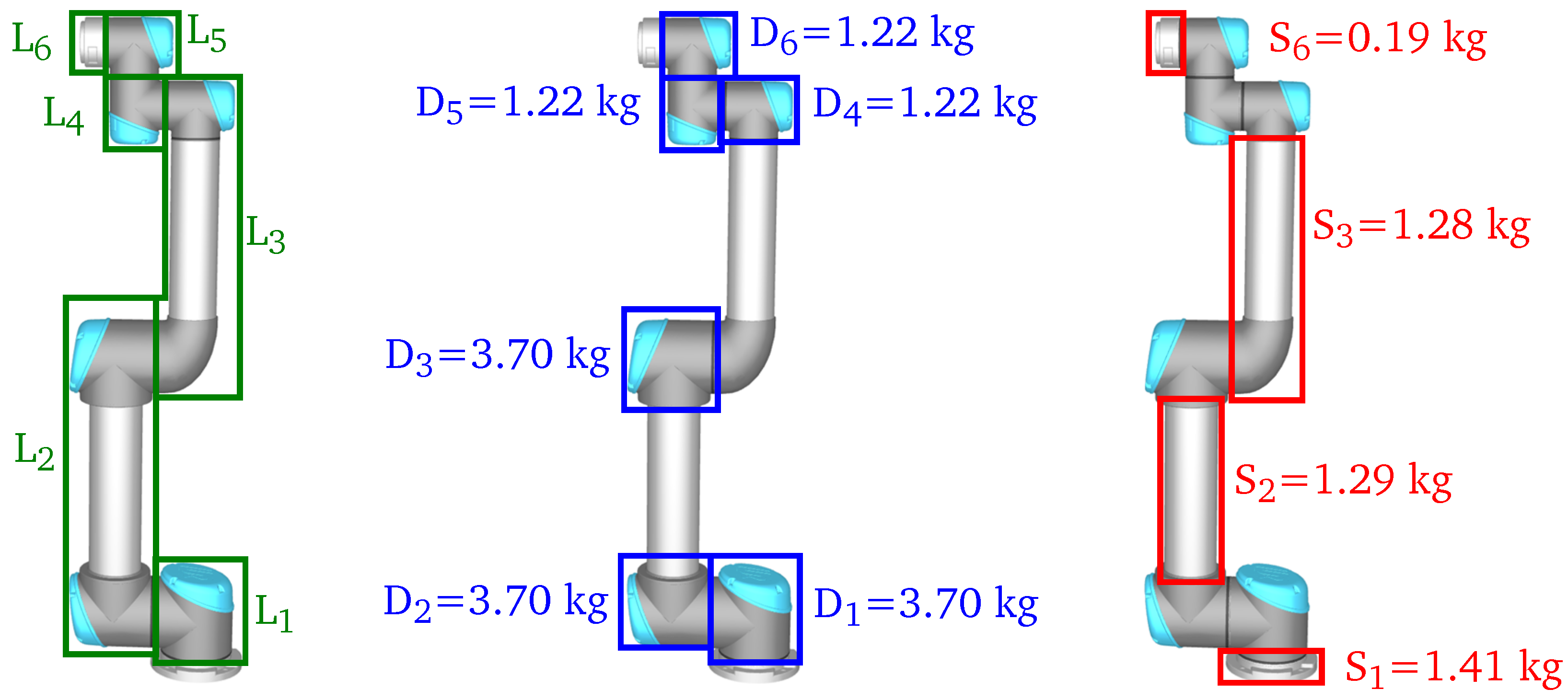
As a basis for the estimation of LCC and the GHG emissions, information of the acquisition and production phase of the robot as well as corresponding spare parts is required. Corresponding information is not publicly available to the best of the authors’ knowledge. Therefore, the robot is analyzed and the modular structure is segmented into one different drive module per joint and structures of each link , as depicted in Figure 3. Thereby, one drive module consists of a motor, motor brake, gear unit and sensors of each joint as well as the corresponding encasement. Based on the diameter of the robot, a larger module is used for and a smaller one is applied for . The remaining components of each link are apportioned to and . Based on the weight of each link and the corresponding components presented in Table A1, Table A2 and Table A3, the weight of the drive modules is estimated. The remaining mass of each link is allocated to the appropriate structural elements. The resulting allocation is depicted in Figure 3. In addition, the weight of the controller of 15 is considered in the LCA. Thereby, the estimated mass of each drive module and segment is only used for the LCA. The dynamic simulation is based on the mass properties of the robot in Table A1 provided by the manufacturer and extended by the rotational inertia of the assumed reducers and motors, as presented in Table A2 and Table A3.
For the modeling of the GHG emissions resulting from the raw material extraction and processing as well as for the country-specific electricity mix, the background database ecoinvent (cutoff model, version 3.7) [32] is integrated into the modeling. It is assumed that the operation phase of the robot system takes place in Germany and thus the German electricity mix is considered. The final product system and the compilation of the life cycle GHG emissions per functional unit is carried out using the software openLCA version 1.10.2. [33]. In the life cycle inventory, the data collection of the modeled product system is carried out. For the production phase, the materials of each component in the drive module, structural element and the controller are estimated and respective data sets are generated. In the life cycle impact assessment, the GHG emissions over the modeled life cycle are compiled using the midpoint impact category Global Warming Potential 100 years according to the impact method IPCC 2013 [34]. The results of the assessment for the production of robot and spare parts are presented in Table 2 based on CO2-equivalents (eq.) and can be used in conjunction with Equation (14) to estimate the environmental impact of the exemplary application.
The costs related to the acquisition and spare parts may vary distinctly depending on the type of robot, additional peripherals or safety equipment, as well as, for example, due to economies of scale. In the following, costs for the acquisition and spare parts are based on assumptions and only serve the clarification of the method. Corresponding estimated values are presented in Table 3. The energy cost rate is taken from [35] for non-household consumers, excluding VAT and other recoverable taxes and levies. Based on the values in Table 3, Equation (13) can be used to estimate the LCC for the exemplary application.
3.2. Evaluation of an Exemplary Task
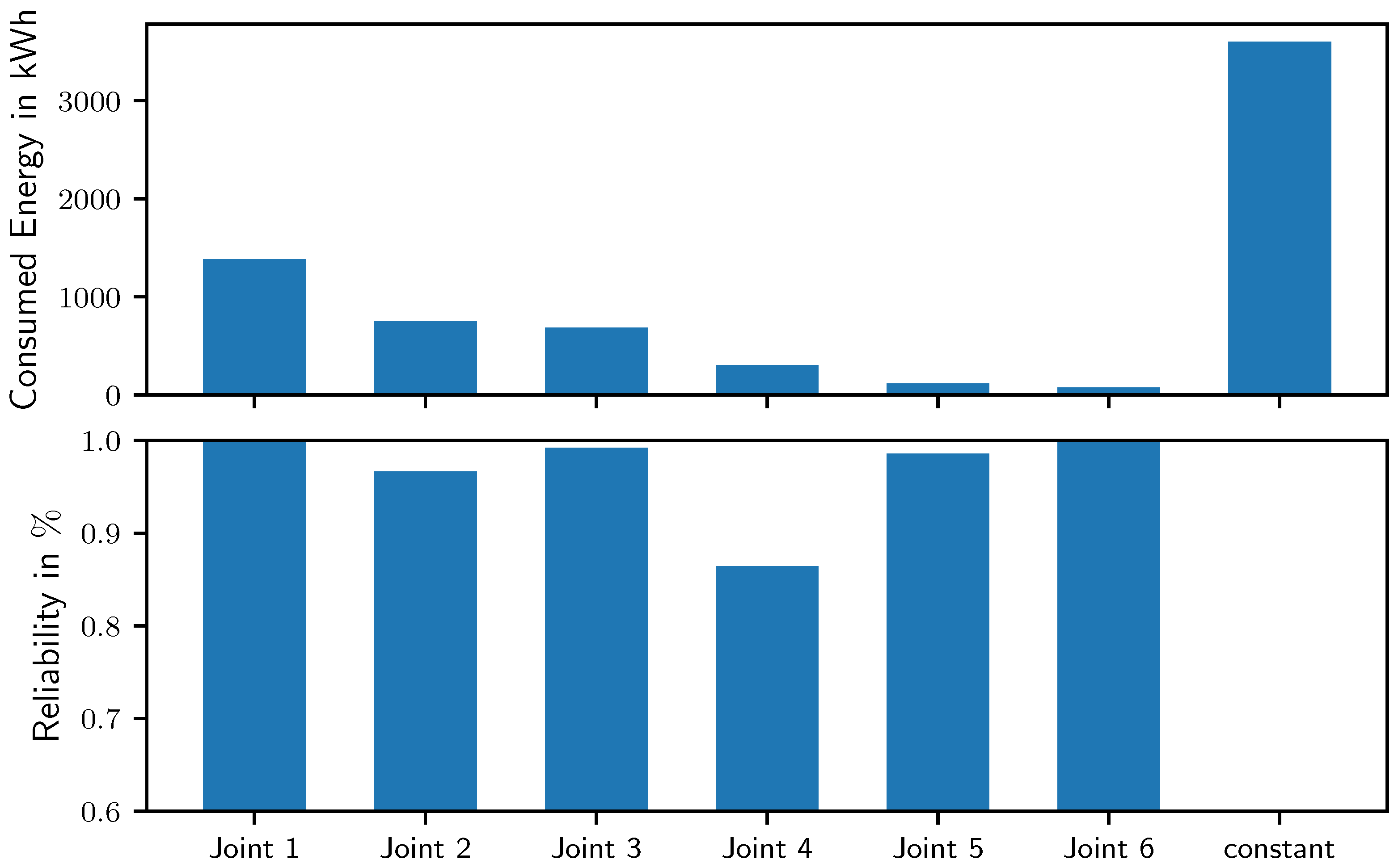
In the following, the task with a duration of and mass of the workpiece is analyzed in detail. Evaluating the trajectory in combination with a constant power consumption of yields an estimated energy consumption of 6913 after = 36,000 h of continuous operation. Analyzing the contribution presented in the top of Figure 4 displays that approximately 50% of the cumulative energy consumption originates from the constant power consumption . Investigating only the impact of the trajectory indicates that joint 1 contributes the most to the total amount, while joints five and six require the least amount. In contrast, the load due to the motion results in decreased reliability of joint two and four, whereby joint four exhibits the lowest reliability as depicted in the bottom of Figure 4. The high load on joint four results from a motion of to change the orientation between and . In contrast to the motion of between and of joint one, the fourth joint is subjected to gravitational loads. Thus, the corresponding load calculated by Equation (8) yields a high strain as a result of the planned trajectory. Hence, based on the analysis of the trajectory, a characteristic distribution of consumed energy and reliability and corresponding critical joints can be determined, allowing one to examine measures to improve resource efficiency. Furthermore, estimating the reliability of each joint may provide a decision support for the selection of a feasible operation time, as well as the number and type of spare parts for a specific task and trajectory.
Based on the reliability of each joint, corrective maintenance is applied and the probabilities of required replacements of the modular joints are determined by a Monte Carlo simulation with 1 × 10⁵ samples. Only considering events with a probability higher than 1% results in the three cases presented in Table 4. With a probability of 81.6%, no repair is required during 36,000 h. Thus, corresponding costs and GHG emissions consist of the acquisition or manufacturing of the robot, as well as the total energy consumed. Evaluating costs and emissions with Equations (13) and (14) yields costs of 36,289 € and CO2-eq. of 4237 . Furthermore, the Monte Carlo simulation yields probabilities of 3.4%, 10.8%, and 1.5% for the replacement of the joint modules , and , respectively. Thus, one small joint module is replaced with a probability of 12.3%, based on the sum of the probabilities of and . Correspondingly, costs and emissions increase by the values of the components based on Table 2 and Table 3.
Based on the considered inputs into the cost functions, the composition of LCC and GHG emissions can be analyzed. Accordingly, the corresponding distributions are partitioned into acquisition or manufacturing, energy consumption and spare parts. In conjunction with the probability of occurrence at the top, Figure 5 presents the resulting composition of LCC in the middle and of GHG emissions in the bottom for each case. The cumulative costs consist of 92% acquisition costs or more for all cases. Costs originating from energy consumption and spare parts account for the remaining percentage depending on each case. In contrast, the energy consumption during the operation contributes 88% or more to the total GHG emissions, while the manufacturing of the robot and the spare parts share the remaining portion. In combination with comparably low probabilities for required replacements, the impact of required spare parts on LCC and GHG emissions is low. As estimated in Table 2 and Table 3, the economic and ecological effects of are lower than for , consequently, the corresponding impact on LCC and GHG emissions differs as well.
Based on the composition, minimizing the energy consumption may provide little reduction in the LCC, but may distinctly reduce the GHG emissions for the selected robot and task. However, additional costs or emissions, e.g., resulting from unplanned downtime, may shift the presented distribution. Furthermore, an increasing utilization of renewable energy may decrease the contribution of energy consumption to the GHG emissions.
3.3. Evaluation of the Impact of Payload and Cycle Time
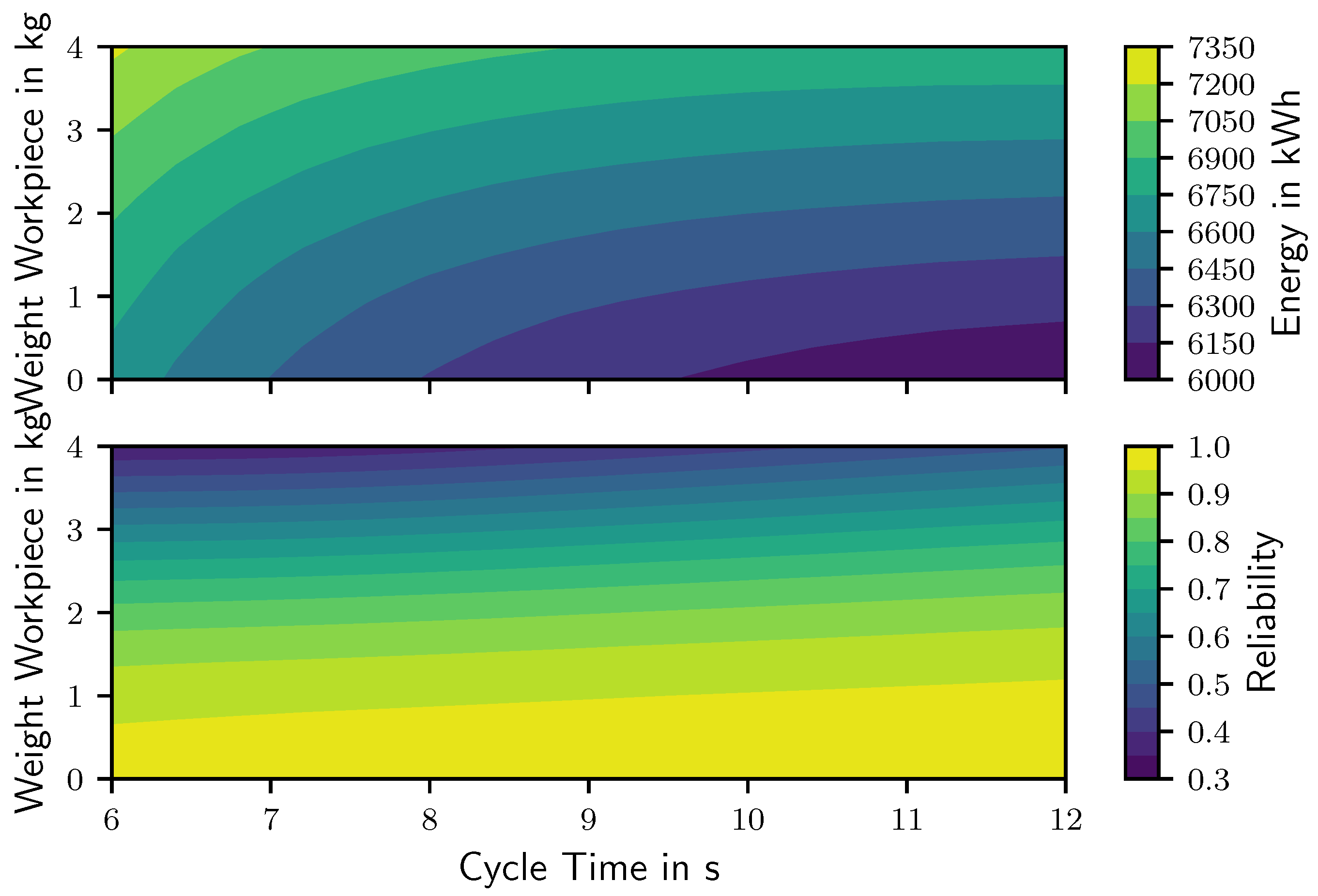
In Ref. [11], a parametric study indicated a distinct impact of the payload and the duration of a single point-to-point motion on energy consumption and expected service life. In the following, a similar study is performed for the selected task and is extended by an analysis of costs and environmental impact. For the parametric study, the weight of the workpiece is varied from 0 to 4 in increments of . Thereby, a workpiece with a weight of 4 in combination with the gripper yields the maximum allowed payload of the robot. For each resulting payload, the cycle time is varied from 6 to 12 in increments of . An overview of the varied parameters is given in Table 5.
Evaluating each combination of workpiece weight and cycle time yields the impact on consumed energy and reliability presented in Figure 6. During a fixed operating time, a higher payload and a quicker motion increase energy consumption and reduce the reliability. Furthermore, the impact of the duration on the consumed energy, especially for short cycle times, is more distinct than the impact of the weight of the workpiece. Overall, the parametric study indicates large variations depending on the weight of the workpiece and the duration of the motion. In addition, a low reliability of 0.3 for tasks with a high payload after 36,000 h of continuous operation may lead to unplanned production stops and may therefore not be reasonable.
For each task and trajectory in the parametric study, a Monte Carlo simulation is performed to determine the number of required replacements for each joint. As the path of the motion is not changed throughout the parametric study, it can be expected that the critical components are and , as discussed for the exemplary task examined in Section 3.2. This is confirmed by the results of the Monte Carlo simulation presented in Figure 7, displaying the probability of the number of required replacements during 36,000 h of continuous operation. Thereby, Figure 7 contains excerpts of the parametric study for selected weights of the workpiece and cycle times. The task with a workpiece weight of 2 and duration of 6 is analyzed in Section 3.2, and similarly to the results presented in Table 4, three cases exist: no replacements are necessary with a probability of 81.6% (blue), while and are replaced once with a probability of 12.4% (orange) and 3.4% (green). For the tasks with a workpiece weight of 0 , events of required replacements occur with probabilities less than 1% (gray) for cycle times of 8 , 10 and 12 . In contrast, for high payloads, the probabilities and the number of relevant cases distinctly increase as a consequence of the low reliability, as already presented in Figure 6. For a workpiece weight of 4 , the Monte Carlo simulation additionally yields events where a component is replaced more than one time or combinations of components have to be repaired.
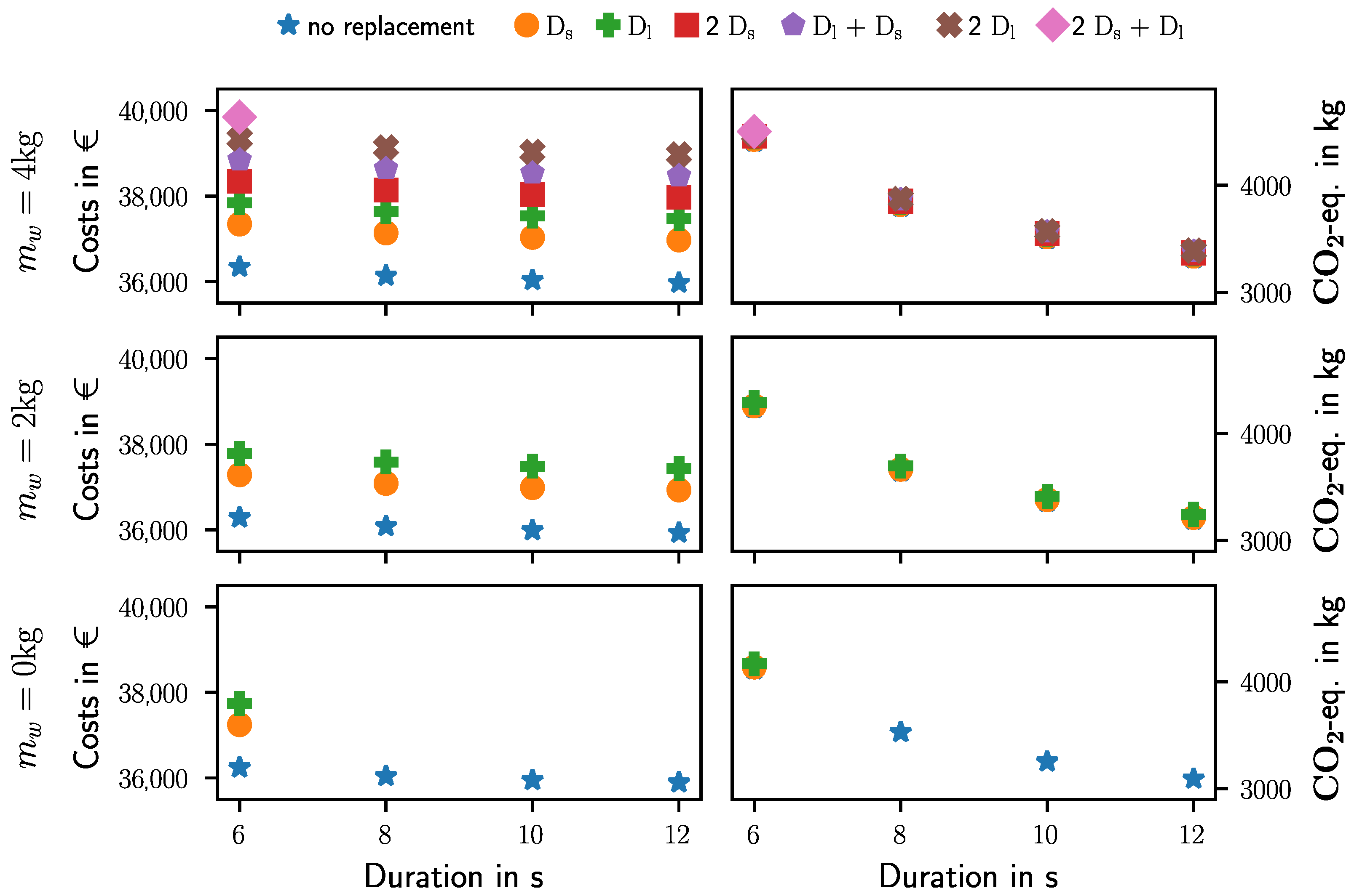
Combining the consumed energy with the results from the Monte Carlo simulation allows one to evaluate the impact of workpiece weight and cycle time on LCC and GHG emissions. Thereby, the respective costs and emissions are plotted in Figure 8 for each relevant case of the Monte Carlo simulation depicted in in Figure 6. Observing the LCC in the left of Figure 8 displays a discrete increase in costs depending on the case and each component’s cost. While the acquisition costs of 35,000 € still account for the largest matter of expense, a high payload may distinctly increase the total costs depending on the number of replacements. The increase in costs depending on payload and cycle time for the same case, e.g., when no replacement is required, is comparably smaller and approximately proportional to the consumed energy. In contrast, short cycle time results in distinctly increased GHG emissions compared to the impact of different amounts of spare parts, as depicted in the right side of Figure 8. This effect can be attributed to a rising energy consumption and its distinct impact on GHG emissions, as discussed for the exemplary task in Section 3.2.
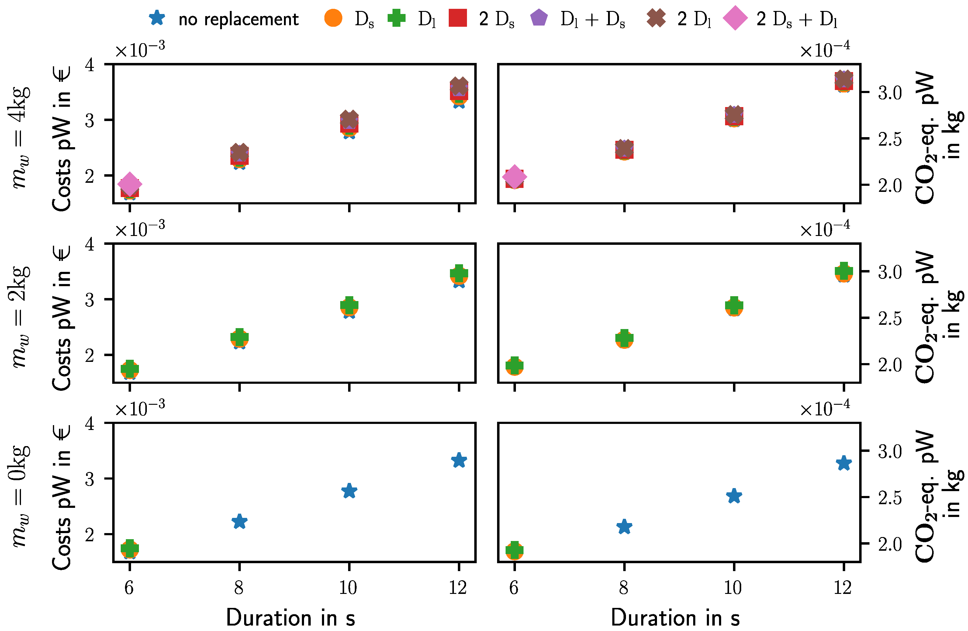
Based on the results presented above, increasing the cycle time would reduce costs and environmental impact. However, this would also lower the productivity of the robotic system. Thus, instead of cumulative costs and emissions, these quantities can be divided by the total amount of workpieces that are transported during 36,000 h of continuous operation. Accordingly, Figure 9 presents the evaluated costs and GHG emissions per workpiece (pW). The costs per workpiece are below 0.005 €, while the emissions are below 3.2 × 10⁻⁴ kg CO2-eq. per workpiece for all tasks and cases. While the increased energy consumption and replacements for short cycle times and high payloads increase the cumulative costs and emissions, Figure 9 displays a distinct dependency of costs and emissions per workpiece depending on the cycle time. Thus, the shortest cycle time yields the lowest LCC and GHG emissions per workpiece for all tasks and cases. However, this may be offset by reduced reliability for short cycle times and a resulting increased probability of unplanned production stops.
To summarize, analyzing energy consumption and reliability in combination with life cycle costing and LCA provides a decision support for the comparison of different systems, tasks or the selection of optimal parameters. Furthermore, the results may differ depending on the objective, as highlighted by the comparison of LCC and GHG emissions with the corresponding impact per workpiece. Nevertheless, it has to be noted that several assumptions and estimated parameters are required for the exemplary task and robot. While this should not affect the general application of the method, the input data need to be adapted for each individual application and results have to be analyzed accordingly. In addition, the impact of the disposal should be considered to complete the life cycle. For the selected task and the presented parametric study, the proposed method provides decision support for the determination of the optimal cycle time. While the weight of the workpiece is usually defined by the task and can not be changed easily, a low reliability for high payloads may, for example, be avoided by the selection of different via-points for the task, an adjusted trajectory or selecting an alternative robot. Correspondingly, various parameters can be adapted to improve the resource efficiency. However, for the application in a production scenario, parameters may be additionally constrained by the production process or depend on the integration with commercial industrial robots. Hence, based on the presented model-based method, variations of relevant decision variables can be generated and evaluated in simulation to assist in the planning stage of a production system.
4. Conclusions
The resource efficiency of industrial robots is a key aspect for the manufacturing industry. While most approaches are focused on minimizing the energy consumption during the use phase, the method presented in this work utilizes the dynamic model of the robot to additionally estimate the reliability of individual components of the robot. This enables the combination of dynamic simulations in conjunction with maintenance methods adapted to a specific application and supported by probabilistic distributions. In this work, corrective maintenance is applied for the assumption that the affected modular joint of the robot is replaced and corresponding probabilities of required replacements are determined via a Monte Carlo simulation. Resulting costs for spare parts are directly considered in the prediction of the LCC based on the amount and type of components replaced. The GHG emissions of a robot performing a task are analyzed with an LCA, thereby the impact of the robot’s manufacture is estimated based on the weights of the links and corresponding components of the actuation system. The use phase is directly considered based on the consumed energy and required spare parts for a specific task and trajectory.
The proposed method is applied to an exemplary robot performing a pick-and-place operation. Analyzing the energy consumption yields a distinct impact of the energy consumed by peripherals and the controller for the selected system, while the first joint exhibits the second largest contribution. In contrast, the fourth joint is identified as a critical component regarding the reliability. Thus, the motion of joint 1 should be adapted to reduce energy consumption, while a manipulation of the motion of joint 4 could improve the reliability and result in a more equally distribution of the reducers’ load. For the selected robot, this may be especially beneficial for high payloads, as indicated by the results of a parametric study. Thereby, the impact of varying workpiece weight and cycle time is investigated regarding energy consumption and reliability, as well as LCC and GHG emissions. The emissions are estimated based on an LCA, considering the manufacturing of the individual components of the robot as well as spare parts and energy consumption. The combination of motion simulation and LCA yields a distinct impact of the consumed energy during the use phase on the GHG emission. Additionally, costs for spare parts are identified as cost drivers for high payloads and short cycle times, as indicated by an associated low reliability. A resulting increase of the cycle time reduces total costs and emissions, while distinctly lowering the total amount of workpieces transported during a fixed amount of operating hours. In contrast, short cycle times yield considerably reduced costs and emissions per workpiece at the cost of decreased reliability.
Combining motion simulations, energy consumption estimation, and reliability prediction with maintenance methods, life cycle costing, and LCA shows great potential to enhance decision-making during production planning or virtual commissioning towards improved resource efficiency. Data from life time tests and enhanced maintenance methods, as well as more detailed estimation of LCC and GHG emissions, can be integrated to improve the accuracy of the prediction. The estimation of a lifetime of components may create possibilities for the re-use of the robot or components. Furthermore, analyzing approaches to reduce energy investigated in literature, e.g., the utilization of compliant elements and regenerative drives, in conjunction with an estimation of the reliability, LCC and GHG emissions may provide further benefits. In addition, extending the strategies for the minimization of the energy consumption to a multi-objective optimizations of task and trajectory, considering that the components’ reliability may further improve the system’s resource efficiency.
Author Contributions
Conceptualization, F.S. and S.W.; methodology, F.S. and S.W.; software, F.S.; validation, F.S. and S.W.; formal analysis, F.S. and S.W.; investigation, F.S. and S.W.; data curation, F.S. and S.W.; writing—original draft preparation, F.S., S.W. and J.J.; writing—review and editing, F.S., S.W., J.J. and D.C.; visualization, F.S.; supervision, L.S., D.C. and S.R.; All authors have read and agreed to the published version of the manuscript.
Funding
This research received no external funding.
Institutional Review Board Statement
Not applicable.
Informed Consent Statement
Not applicable.
Acknowledgments
We acknowledge support by the German Research Foundation and the Open Access Publishing Fund of Technical University of Darmstadt.
Conflicts of Interest
The authors declare no conflict of interest.
Abbreviations
The following abbreviations are used in this manuscript:
| LCC | Life Cycle Costs |
| LCA | Life Cycle Assessment |
| GHG | Greenhouse Gas |
Appendix A. UR5 Robot and Drive Train Parameters

Table A1.
Mass properties and Denavit-Hartenberg Parameters of the UR5 [36].
Table A1.
Mass properties and Denavit-Hartenberg Parameters of the UR5 [36].
| Link/Joint | Mass in kg | Center of Mass in m | θ in rad |
| 1 | 0 | ||
| 2 | 0 | ||
| 3 | 0 | ||
| 4 | 0 | ||
| 5 | 0 | ||
| 6 | 0 | ||
| Link/Joint | a in m | d in m | in |
| 1 | 0 | 0.089159 | |
| 2 | −0.425 | 0 | 0 |
| 3 | −0.39225 | 0 | 0 |
| 4 | 0 | 0.10915 | |
| 5 | 0 | 0.09465 | |
| 6 | 0 | 0.823 | 0 |
Table A2.
Properties of the reducer, based on the family HFUS-2SH [18].
Table A2.
Properties of the reducer, based on the family HFUS-2SH [18].
| Joints | Size | ig | Mass in kg | Inertia in kg m2 |
| 1, 2, 3 | 25 | 100 | 1.44 | 1.07 × 10⁻⁴ |
| 4, 5, 6 | 14 | 100 | 0.45 | 9.1 × 10⁻⁶ |
| Joints | Lr in h | in rad/s | ur in N m | c |
| 1, 2, 3 | 3.5 × 10⁴ | 1.152 | 67 | 3 |
| 4, 5, 6 | 3.5 × 10⁴ | 1.152 | 7.8 | 3 |
Table A3.
Properties of the motor with friction brake, based on the RDU family based on [37].
Table A3.
Properties of the motor with friction brake, based on the RDU family based on [37].
| Joints | Size | Mass in kg (Estimated) | Inertia in kg m2 | km in N m/A |
| 1, 2, 3 | 70 × 18-HW | 0.71 | 9 × 10⁻⁵ | 0.106 |
| 4, 5, 6 | 50 × 08-HW | 0.24 | 2.5 × 10⁻⁵ | 0.057 |
| Joints | Size | kb in V s/rad | L in H | R in Ω |
| 1, 2, 3 | 70 × 18-HW | 0.106 | 7.2 × 10⁻⁴ | 0.552 |
| 4, 5, 6 | 50 × 08-HW | 0.057 | 8 × 10⁻⁴ | 0.47 |
Table A4.
Estimated friction parameters of the reducer, based on the family HFUS-2SH [18].
Table A4.
Estimated friction parameters of the reducer, based on the family HFUS-2SH [18].
| Joints | Bc in N m (Estimated) | Bv in N m s/rad (Estimated) |
|---|---|---|
| 1, 2, 3 | 20.32 | 11.94 |
| 4, 5, 6 | 3.37 | 2.0 |
References
- Kagermann, H. Recommendations for Implementing the Strategic Initiative INDUSTRIE 4.0: Securing the Future of German Manufacturing Industry; Final Report of the Industrie 4.0 Working Group; Forschungsunion: Berlin, Germany, 2013. [Google Scholar]
- Schebek, L.; Kannengießer, J.; Campitelli, A.; Fischer, J.; Abele, E.; Bauerdick, C.; Anderl, R.; Haag, S.; Sauer, A.; Mandel, J.; et al. Studie: Ressourceneffizienz durch Industrie 4.0—Potenziale für Kleine und Mittlere Unternehmen (KMU) des Verarbeitenden Gewerbes, vdi zre publikationen ed.; Studien, VDI Publikationen: Berlin, Germany, 2017. [Google Scholar]
- Pellicciari, M.; Avotins, A.; Bengtsson, K.; Berselli, G.; Bey, N.; Lennartson, B.; Meike, D. AREUS—Innovative Hardware and Software for Sustainable Industrial Robotics. In Proceedings of the 2015 IEEE International Conference on Automation Science and Engineering (CASE), Gothenburg, Sweden, 24–28 August 2015; pp. 1325–1332. [Google Scholar]
- Meike, D.; Pellicciari, M.; Berselli, G. Energy Efficient Use of Multirobot Production Lines in the Automotive Industry: Detailed System Modeling and Optimization. IEEE Trans. Autom. Sci. Eng. 2014, 11, 798–809. [Google Scholar] [CrossRef]
- Bukata, L.; Šůcha, P.; Hanzálek, Z.; Burget, P. Energy Optimization of Robotic Cells. IEEE Trans. Ind. Inform. 2017, 13, 92–102. [Google Scholar] [CrossRef]
- Carabin, G.; Wehrle, E.; Vidoni, R.; Carabin, G.; Wehrle, E.; Vidoni, R. A Review on Energy-Saving Optimization Methods for Robotic and Automatic Systems. Robotics 2017, 6, 39. [Google Scholar] [CrossRef] [Green Version]
- Dijkman, T.J.; Rödger, J.; Bey, N. How to Assess Sustainability in Automated Manufacturing. In Proceedings of the 2015 IEEE International Conference on Automation Science and Engineering (CASE), Gothenburg, Sweden, 24–28 August 2015; pp. 1351–1356. [Google Scholar]
- Wyatt, H.; Wu, A.; Thomas, R.; Yang, Y. Life Cycle Analysis of Double-Arm Type Robotic Tools for LCD Panel Handling. Machines 2017, 5, 8. [Google Scholar] [CrossRef] [Green Version]
- Yamada, A.; Takata, S. Reliability Improvement of Industrial Robots by Optimizing Operation Plans Based on Deterioration Evaluation. CIRP Ann. 2002, 51, 319–322. [Google Scholar] [CrossRef]
- Lin, C.-Y.; Zhao, Y.; Tomizuka, M.; Chen, W. Path-Constrained Trajectory Planning for Robot Service Life Optimization. In Proceedings of the 2016 American Control Conference (ACC), Boston, MA, USA, 6–8 July 2016; pp. 2116–2122. [Google Scholar]
- Stuhlenmiller, F.; Jungblut, J.; Clever, D.; Rinderknecht, S. Combined Analysis of Energy Consumption and Expected Service Life of a Robotic System. In Proceedings of the 2020 6th International Conference on Mechatronics and Robotics Engineering (ICMRE), Barcelona, Spain, 12–15 February 2020; pp. 53–57. [Google Scholar]
- Müller, A.; Bornschlegl, M.; Kettelmann, P.; Mantwill, F.; Müller, O. Digital Planning of Complex Production Systems Based on Life-Cycle Costs. In Proceedings of the IECON 2018—44th Annual Conference of the IEEE Industrial Electronics Society, Washington, DC, USA, 21–23 October 2018; pp. 3033–3038. [Google Scholar]
- Landscheidt, S.; Kans, M. Method for Assessing the Total Cost of Ownership of Industrial Robots. Procedia CIRP 2016, 57, 746–751. [Google Scholar] [CrossRef]
- Boscariol, P.; Caracciolo, R.; Richiedei, D.; Trevisani, A. Energy Optimization of Functionally Redundant Robots through Motion Design. Appl. Sci. 2020, 10, 3022. [Google Scholar] [CrossRef]
- Lynch, K.M.; Park, F.C. Modern Robotics: Mechanics, Planning, and Control, 1st ed.; Cambridge University Press: Cambridge, UK, 2017. [Google Scholar]
- Olsson, H.; Åström, K.; de Wit, C.C.; Gäfvert, M.; Lischinsky, P. Friction Models and Friction Compensation. Eur. J. Control 1998, 4, 176–195. [Google Scholar] [CrossRef] [Green Version]
- Wahrburg, A.; Klose, S.; Clever, D.; Groth, T.; Moberg, S.; Styrud, J.; Ding, H. Modeling Speed-, Load-, and Position-Dependent Friction Effects in Strain Wave Gears. In Proceedings of the 2018 IEEE International Conference on Robotics and Automation (ICRA), Brisbane, QLD, Australia, 21–25 May 2018; pp. 2095–2102. [Google Scholar]
- Harmonic Drive AG. Engineering Data HFUS-2UH/2SO/2SH Units. Available online: https://harmonicdrive.de/de/downloads (accessed on 18 November 2020).
- Gadaleta, M.; Berselli, G.; Pellicciari, M.; Sposato, M. A Simulation Tool for Computing Energy Optimal Motion Parameters of Industrial Robots. Procedia Manuf. 2017, 11, 319–328. [Google Scholar] [CrossRef]
- Paes, K.; Dewulf, W.; Elst, K.V.; Kellens, K.; Slaets, P. Energy Efficient Trajectories for an Industrial ABB Robot. Procedia CIRP 2014, 15, 105–110. [Google Scholar] [CrossRef] [Green Version]
- Takata, S.; Yamada, A.; Kohda, T.; Asama, H. Life Cycle Simulation Applied to a Robot Manipulator—An Example of Aging Simulation of Manufacturing Facilities. CIRP Ann. 1998, 47, 397–400. [Google Scholar] [CrossRef]
- Pettersson, M.; Ölvander, J. Drive Train Optimization for Industrial Robots. IEEE Trans. Robot. 2009, 25, 1419–1424. [Google Scholar] [CrossRef]
- Zhou, L.; Bai, S. A New Approach to Design of a Lightweight Anthropomorphic Arm for Service Applications. J. Mech. Robot. 2015, 7, 031001. [Google Scholar] [CrossRef]
- Bertsche, B. Reliability in Automotive and Mechanical Engineering; Springer: Berlin/Heidelberg, Germany, 2008. [Google Scholar]
- Wang, H.; Pham, H. Reliability and Optimal Maintenance; Springer Series in Reliability Engineering; Springer: London, UK, 2006. [Google Scholar]
- Zhang, C.; Wang, S.; Wang, Z.; Wang, X. An Accelerated Life Test Model for Harmonic Drives under a Segmental Stress History and Its Parameter Optimization. Chin. J. Aeronaut. 2015, 28, 1758–1765. [Google Scholar] [CrossRef] [Green Version]
- Schmidt, J.; Schmid, M. Life Test of an Industrial Standard and of a Stainless Steel Harmonic Drive. In Proceedings of the 14th European Space Mechanisms & Tribology Symposium—ESMATS 2011, Constance, Germany, 28–30 September 2011; p. 8. [Google Scholar]
- Mobley, J.; Parker, J. Harmonic Drive—Gear Material Selection and Life Testing. In Proceedings of the 41st Aerospace Mechanism Symposium, Pasadena, CA, USA, 16–18 May 2012; p. 14. [Google Scholar]
- ISO 281:2007-02. Rolling Bearings—Dynamic Load Ratings and Rating Life; International Organization for Standardization: Geneva, Switzerland, 2007. [Google Scholar]
- ISO 14040:2009-011. Environmental Management—Life Cycle Assessment—Principles and Framework; International Organization for Standardization: Geneva, Switzerland, 2009. [Google Scholar]
- ISO 14044:2006. Environmental Management—Life Cycle Assessment—Requirements and Guidelines; International Organization for Standardization: Geneva, Switzerland, 2006. [Google Scholar]
- Weidema, B.P.; Bauer, C.; Hischier, R.; Mutel, C.; Nemecek, T.; Reinhard, J.; Vadenbo, C.O.; Wernet, G. Overview and Methodology: Data Quality Guideline for the Ecoinvent Database Version 3; Ecoinvent Report 1(v3); The Ecoinvent Centre: St. Gallen, Switzerland, 2013. [Google Scholar]
- Green Delta GmbH. openLCA—The Life Cycle and Sustainability Modeling Suite. Available online: https://www.openlca.org (accessed on 12 October 2020).
- Intergovernmental Panel on Climate Change. Climate Change 2013: The Physical Science Basis. Contribution of Working Group I to the Fifth Assessment Report of the Intergovernmental Panel on Climate Change. Available online: https://www.ipcc.ch/site/assets/uploads/2018/02/WG1AR5_all_final.pdf (accessed on 18 October 2020).
- Eurostat, Electricity Prices for Non-Household Consumers—Bi-Annual Data. Available online: http://appsso.eurostat.ec.europa.eu/nui/submitViewTableAction.do (accessed on 18 November 2020).
- Universal Robots A/S. Parameters for Calculations of Kinematics and Dynamics. Available online: https://www.universal-robots.com/articles/ur/parameters-for-calculations-of-kinematics-and-dynamics/ (accessed on 24 November 2020).
- TQ-Systems GmbH. RoboDrive Hollow Shaft Servomotors RDU70x18-HW. Available online: https://www.tq-group.com/en/products/tq-robodrive/servomotors/rdu70x18-hw/ (accessed on 24 November 2020).
Figure 1.
Exemplary task analyzed in this study: the configuration for picking up and for placing a sphere as the workpiece is presented in the left and right, respectively. The trace is depicted in yellow.
Figure 1.
Exemplary task analyzed in this study: the configuration for picking up and for placing a sphere as the workpiece is presented in the left and right, respectively. The trace is depicted in yellow.

Figure 2.
Curve fit of failure probability for the strain wave gear based on life adjustment factors for reliability from ISO 281.
Figure 2.
Curve fit of failure probability for the strain wave gear based on life adjustment factors for reliability from ISO 281.

Figure 3.
Segments and their estimated mass for the UR5.

Figure 4.
Overview of the energy consumption and reliability for each joint after 36,000 h of operation.
Figure 4.
Overview of the energy consumption and reliability for each joint after 36,000 h of operation.

Figure 5.
Composition of LCC and GHG emissions after 36,000 h of continuous operation.

Figure 6.
Consumed energy and reliability after 36,000 h of continuous operation depending on the weight of the workpiece and the duration of one cycle.
Figure 6.
Consumed energy and reliability after 36,000 h of continuous operation depending on the weight of the workpiece and the duration of one cycle.

Figure 7.
Probability of the number of repairs, depending on the component of the robot during 36,000 h of continuous operation.
Figure 7.
Probability of the number of repairs, depending on the component of the robot during 36,000 h of continuous operation.

Figure 8.
LCC and GHG emissions after 36,000 h of continuous operation considering possible repairs depending on the load of the workpiece and the duration of the cycle.
Figure 8.
LCC and GHG emissions after 36,000 h of continuous operation considering possible repairs depending on the load of the workpiece and the duration of the cycle.

Figure 9.
LCC and GHG emissions per workpiece (pW) after 36,000 h of continuous operation considering possible repairs, depending on the load of the workpiece and the duration of the cycle.
Figure 9.
LCC and GHG emissions per workpiece (pW) after 36,000 h of continuous operation considering possible repairs, depending on the load of the workpiece and the duration of the cycle.

Table 1.
Locations, Orientations and Configurations of the Task.
| Point | Location (w.r.t. Robot Base) in m | Euler Angles (rpy) in rad |
| Point | Joint Angles in | |
Table 2.
Estimated GHG emissions for the manufacturing of the robot.
| Component | CO2-eq. in kg | CO2-eq. in of Total |
|---|---|---|
| 11.3 | ||
| 4.7 | ||
| Structure | 91.1 | 19.7 |
| Control Box | 149.3 | 32.3 |
| Robot | 100 | |
| Emission factor for the electricity mix: | 0.5459 kg/kWh CO2-eq. (ee) | |
Table 3.
Overview of the items of expenses.
| Acquisition | Spare Part Dl | Spare Part Ds | Electricity Pricing |
|---|---|---|---|
| 35,000 € | 1.500 € | 1.000 € | 0.186 € |
Table 4.
Overview of the LCC and GHG emissions after 36,000 h of operation.
| Parts to Replace | Probability in % | Costs in € | CO2-eq. in kg |
|---|---|---|---|
| − | 81.6 | 36,289 | 4237 |
| 12.3 | 37,289 | 4259 | |
| 3.4 | 37,789 | 4289 |
Table 5.
Overview of varied parameters in the parametric study.
| Parameter | Min | Max | Increment |
|---|---|---|---|
| in | 0 | 4 | 0.2 |
| in | 6 | 12 | 0.4 |
Publisher’s Note: MDPI stays neutral with regard to jurisdictional claims in published maps and institutional affiliations. |
© 2021 by the authors. Licensee MDPI, Basel, Switzerland. This article is an open access article distributed under the terms and conditions of the Creative Commons Attribution (CC BY) license (http://creativecommons.org/licenses/by/4.0/).
Share and Cite
MDPI and ACS Style
Stuhlenmiller, F.; Weyand, S.; Jungblut, J.; Schebek, L.; Clever, D.; Rinderknecht, S. Impact of Cycle Time and Payload of an Industrial Robot on Resource Efficiency. Robotics 2021, 10, 33. https://doi.org/10.3390/robotics10010033
AMA Style
Stuhlenmiller F, Weyand S, Jungblut J, Schebek L, Clever D, Rinderknecht S. Impact of Cycle Time and Payload of an Industrial Robot on Resource Efficiency. Robotics. 2021; 10(1):33. https://doi.org/10.3390/robotics10010033
Chicago/Turabian StyleStuhlenmiller, Florian, Steffi Weyand, Jens Jungblut, Liselotte Schebek, Debora Clever, and Stephan Rinderknecht. 2021. "Impact of Cycle Time and Payload of an Industrial Robot on Resource Efficiency" Robotics 10, no. 1: 33. https://doi.org/10.3390/robotics10010033
Note that from the first issue of 2016, this journal uses article numbers instead of page numbers. See further details here.