On Double Value at Risk


1
School of Science, Nanjing University of Science and Technology, Nanjing 210094, China
2
Securities Co., Ltd., Beijing 102627, China
*
Author to whom correspondence should be addressed.
†
These authors contributed equally to this work.
Risks 2019, 7(1), 31; https://doi.org/10.3390/risks7010031
Submission received: 10 February 2019
/
Revised: 2 March 2019
/
Accepted: 5 March 2019
/
Published: 8 March 2019
Abstract
:Value at Risk (VaR) is used to illustrate the maximum potential loss under a given confidence level, and is just a single indicator to evaluate risk ignoring any information about income. The present paper will generalize one-dimensional VaR to two-dimensional VaR with income-risk double indicators. We first construct a double-VaR with (or ) indicators, and deduce the joint confidence region of (or ) by virtue of the two-dimensional likelihood ratio method. Finally, an example to cover the empirical analysis of two double-VaR models is stated.
1. Introduction
In the early 1990s, the international economic and financial consultancy G30 published the report “derivatives practices and principles” based on the research on financial derivatives, and then proposed Value at Risk (VaR) model to measure the market risk. JP Morgan Bank then launched the VaR risk measurement and control model. Since VaR is accurate and comprehensive to the application of risk measurement and makes up the deficiency of Markowitz mean-variance model, it is generally welcomed by the international financial community, including regulatory authorities, and has become a standard to manage and control financial risk. Furthermore, VaR is widely used to measure credit risks and trading risks.
The biggest benefit of VaR is the ability to critically analyze risk through systematic analysis. The organization can control the front end and back end of the business by calculating VaR to understand the financial risks it faces and establish an independent risk management mechanism.
However, VaR also has its own limitations. Mausser and Rosen (1999) put forward the most obvious limitations of VaR: it does not provide absolute maximum loss value, which can only be expected in a certain confidence level. Another drawback of VaR is that when the calculation is based on historical data, the future situation of any event should be duplicated or fitted by historical data. However, the reality is that we cannot guarantee the future case of an event is just as old as. In addition, some researchers such as Artzner et al. (1999) criticized the VaR model because it does not meet sub-additivity.
The obvious limitation existing in VaR is that it is only used to illustrate the maximum possible loss for the given conditions and is only a single index to characterize the risk, which provides less information to users about other information such as income. In practice, what people usually care about is how much profit they can get while taking risks.
Based on the above considerations, we hope to follow the definition of VaR and Markowitz’s portfolio theory, and then construct a double-VaR, that is, we will extend one-dimensional single-risk monitoring indicator-VaR to two-dimensional revenue-risk monitoring indicators-VaR (or double-VaR for short).
There is abundant literature about VaR. Here, the main research literature involved in this paper is described briefly as follows.
Duffie and Pan (1997) made a detailed background description of VaR, characteristics, applications, and the entire VaR-system. Beder (1995) used eight different models to calculate VaR values and compare them. Some foreign scholars studied mainly the calculation of VaR, such as Jorion (1996); Linsmeier and Pearson (1996); Duffie and Pan (1997); Engle and Manganelli (1999). Based on different situations, they arrived at many calculation skills such as the variance-covariance matrix method, historical simulation, and Monte Carlo simulation method, and the related characteristics of VaR, etc.
After 1999, there are an increasing number of new VaR models in the financial, industrial, and other different applied areas. Potters and Bouchaud (1999) proposed how to use the normality of asset volatilities to calculate the VaR of nonlinear combination. Some other scholars studying the nature of VaR and other risk measurement methods, such as Artzner et al. (1999), proposed VaR does not meet sub-additivity; Wang (1999) studied the characteristics of dynamic risk measures; Mausser and Rosen (1999) proposed that if a small-probability event happened in the case of loss exceeding the VaR, then VaR models cannot measure the size of potential losses; Chen et al. (2014) studied future cash arbitrage with VaR-portfolio problems; Tang et al. (2018) investigated the no-arbitrage problem with VaR-like arguments; Cong and Zhao (2018; 2019) posed a non-cash risk measure and a generalized non-cash risk measure, respectively, which improved in some sense VaR under the distribution of any random variable that is uncertain. In addition, some scholars extended the classical Markowitz mean-variance model to the mean-VaR model; for instance, Pearson (2002) and Jorion (2007) used these models with constraints to manage the risk-profit for a fund company.
In addition, many scholars have proposed a series of improved calculation methods based on different markets and different assumptions. Berkowitz (1999) proposed a new method for evaluation of VaR. Taylor et al. (2000) proposed to use the t distribution to fit the income sequence; Hu (2012) based their research on the mixed Copula model to study the evaluation value of VaR; Ze-To (2013) used the Heath-Jarrow-Morton model to measure the value of VaR, and pointed out that the model can capture the non-normal income distribution well and can accurately provide the value of VaR; Li et al. (2017) confirmed that using the Bootstrap method to calculate VaR and CVaR can effectively improve the estimation accuracy.
Meanwhile, many foreign scholars have also attached great importance to the empirical applications of VaR. Jackson et al. (1997) studied how to apply VaR into bank reserves. Berkowitz and O’Brien (2002) proposed how to evaluate the transaction risk of commercial banks through the prediction accuracy of the VaR model. Basak and Shapiro (2001) analyzed the optimal dynamic portfolio risks with VaR model.
In the present paper, we will extend one-dimensional single-risk monitoring indicator—VaR—to two-dimensional benefit-risk monitoring indicators—double-VaR.
Firstly, a reasonable definition of two-dimensional VaR (double-VaR) is given. For a better understanding of double-VaR we choose mean and variance as the parameters to build the first double-VaR model. Thus, for a given confidence level , one can not only know the scope of asset risks but also can know their income range. Such indicators are better able to make trade-offs to the risk-return of assets.
Secondly, to solve the first model—double-VaR with respect to —we extend the one-dimensional likelihood ratio method to two-dimensional likelihood ratio method, and derive the joint confidence region containing the unknown parameters. Then, we can solve a specific joint confidence region with ideal point method and area minimization method as well as to compare the results of these two methods.
Finally, according to the accuracy theory of VaR we study the double-VaR based on so that for a given confidence interval we cannot only know the biggest value of possible asset loss but we can also get the gain range. In this situation a better trade-off of the asset is possible.
2. Preliminaries
2.1. VaR
2.1.1. Definitions and Basic Descriptions
Definition 1.
The basic meaning of VaR is the maximum potential loss of risk assets under normal market conditions, for a given confidence level α and holding period t. One can describe it as follows
where is the loss of risk asset W within the holding period t and VaR is the value at risk under the confidence level α.
Remark 1.
Under a normal market environment and a given confidence level α, let the probability distribution density function of a risky asset value be , the initial value of a risky asset be , the lowest value of a risky asset under a confidence level α be and the yield on holding period t be r, then we have
where and can be achieved with the following two formulas
In particular, when the distribution of the risk asset yield r is a normal distribution, that is, , then one can get VaR of the risk asset by the following steps:
Let
where is the probability density function of a standard normal distribution. According to (2) and (3), we can get
where is the normal probability density function of the risk asset with yield r. Since one has
and
where and . We arrive here by (4) and (5)
More generally, if one considers the time factor for VaR, then the Formula (8) can be written as .
In other words, when the yield on a risk asset follows a normal distribution, VaR measure of the risk is equivalent to the variance measure.
2.1.2. Properties of VaR
VaR has the following properties:
(1) Transformation invariance
For any and positive x, there holds
(2) Positive homogeneity
For any , there holds
(3) Co-monotonic additivity
For any is co-monotonic, there holds
(4) First-order stochastic dominance
For , if the first order of x is better than that of y, there holds
(5) Discontinuity on the confidence level
With respect to the confidence level , VaR is not continuous.
(6) Convexity is not satisfied
This property means that the local minimizer of an optimizing problem with VaR as an objective function is not unique.
(7) Sub-additivity is not satisfied
This means that VaR for a portfolio is not less than the sum of VaR of all risky assets.
3. Double-VaR
3.1. Introduction of Double-VaR
We now chose the mean and variance as two proposed parameters-based on Markowitz’s portfolio theory to form a revenue-risk region D. Then we can define VaR-like as follows
Remark 2.
It is not hard to speculate that the role of the revenue-risk region D in fact is similar to that of VaR. For convenience, we may call the boundary (or partial boundary) of D a double-VaR with respect to indexes μ and . A detailed definition of double-VaR will be given later.
Its real economic significance is under the normal market environment and a given confidence level, an area in which the maximum possible loss (expressed by var ) and the benefits (expressed by mean μ) of an asset within a certain time in the future falls.
3.2. Double-VaR Model with Respect to
3.2.1. Two-Dimensional Likelihood Ratio Argument
Chen and Jiang (2017) proposed and studied a high-dimensional likelihood method for normal distribution. However, for the use of the two-dimensional likelihood method for the derivation of the joint confidence domain, we have not found relevant literature. Thus, we innovate based on learning their ideas to solve the two-dimensional joint confidence region for double-VaR problem.
Assume that the total distribution of follows a distribution whose density function is , where the parameters are unknown. For the given sample observations, it is easy to get the likelihood function:
If the maximum likelihood estimation of is that is, , is the parameter space of , the likelihood ratio can be defined as
For a given confidence level, the joint confidence region D of the parameter can be calculated by R.
When the total , where is a set of sample values and the confidence level is , the joint confidence region of can be gained by the following two-dimensional likelihood ratio, where the unknown parameter is .
In fact, we have known the maximum likelihood estimations of mean and variance are respectively by and . Then we get
Next we can get the likelihood ratio
Since
Denote by and , thus we get the following
Substitute the formula above into (9) and get
Since
and , if we let , then there holds . Since
and . Let , we arrive at . For convenience, we denote by
It is obvious that there holds
By a sufficient condition of two-dimensional extreme points, we can know R has a strict maximum at the point . Thus, for the constant C, there exists a region D so that . According to the meaning of likelihood ratio, let , then . Since
there exist three positive constants and , so that
Since two statistics are , there holds
That is
where is the function value of distribution whose freedom is at the point b. Arrange (10) and get the joint confidence region of as below
Obviously, there are unknowns a, b, and c in the joint confidence domain under the confidence level required by this paper. Therefore, to find these three unknowns, we can determine the specific joint confidence domain after given n and sample variance.
Definition 2.
Assume that is a random vector, and are two index parameters, for given confidence level , one can define double-VaR of with respect to indexes as
In the above definition, a, b, c are unknown. However, in Section 3.2.2, we use the ideal method to find the joint confidence domain. Thus, the unknown parameters a, b, c are solved. We can look up Table 1 and Table 2 to find the value of a, b, c.
Remark 3.
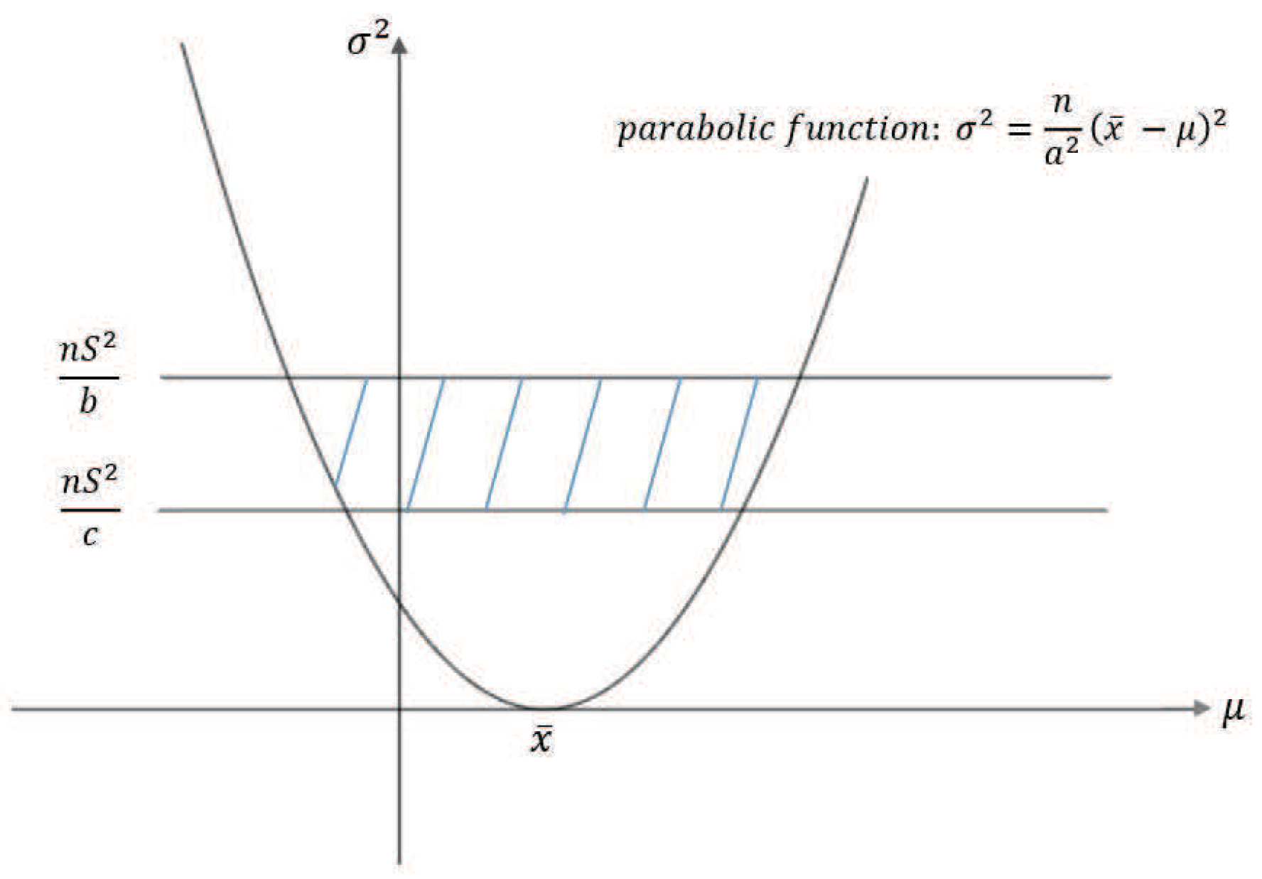
Noticing that the joint confidence region (see Figure 1 below) and combining with Markowitz’s portfolio theory, the right boundary of the banded region in Figure 1 can be regarded the dobule-VaR, , with .
That is to say, one can have the following two basic understandings:
(1) For a given risk level , can be regarded as VaR in the sense of Markowitz’s portfolio with a given confidence level α;
(2) For a given benefit level , can also be regarded as VaR in the sense of Markowitz’s portfolio with a given confidence level α.
3.2.2. Solution to Joint Confidence Region on
We adopt the so-called ideal point method to solve the joint confidence region.
It is well known that the joint confidence region of is just as (12). It is now we evaluate and c.
Firstly, one can analyze Figure 1 of this joint confidence region of as below:
Given the confidence level , to minimize the area of this joint confidence region, it implies that if the two straights and deciding the size of shaded area are closed enough, which shows and . At the same time, we hope to make the parabolic narrower, that is, one considers the problem: and . The parabolic can be regarded as an effective frontier of Markowitz portfolio in -coordinate system.
Then we need to solve the following optimization model
To solve problem (13), we first refer consider three single-objective optimization models, respectively, as follows
After knowing n and the variance of samples , these three optimization problems can be simplified as below
Now assume that the solutions of these three problems above are respectively denoted by , , . We set and call it an ideal point of (13), but it is obvious that the ideal point is not necessarily a solution to (13). In fact, we want to get the Euclidean distance between this extremum point and the ideal point is as small as possible. That is, we wish to consider the following
There is also a point that deserves to be noticed in the theory of probability and statistics when the variance of population is unknown; estimating the mean of population can be divided into two cases:
(1) When the number of sample observations is less than 30, we often choose t distribution to make a parameter estimation of the mean; when the number of sample observations is more than 30, we chose the normal distribution to estimate the parameters. To have a more accurate estimation the number of observations of more than 30 in this article, so we will use the normal distribution to estimate the mean in the process of solving the joint confidence region.
In addition, we notice that freedom n is usually less than 45 in any distribution, because when n is more than 45 it is close to a normal distribution . Thus, this article first studies the case when .
(2) When the number of sample observations is , we will make a further study.
3.3. Double-VaR Model Based on
According to the theory of VaR, we will consider the joint confidence region of is reasonable and significant.
3.3.1. Accuracy Measurement of VaR
By the description in Section 2.1.1, we can know , that is, if the initial value of asset and the confidence level has been known, VaR is only related to standard deviation . Because is decided by the choice of sample observations there exits statistical errors in the solving of VaR. Different lengths of confidence sections provide different accuracy of VaR. It is very important to get the length of the confidence section.
3.3.2. -Model
According to the definition of joint confidence region we have
where D is the joint confidence region of when the confidence level has been known. In particular, the given confidence level of the joint confidence region of is not related to the confidence level of VaR itself . If the confidence level of VaR is 99% and the confidence level of the joint confidence region of is 95%, the object studied in this article can be explained as: the return of an asset in one day and the biggest 99% loss of VaR are in the area D with the probability 95%.
When the total , are a set of sample values and the confidence level is , the joint confidence region of can be gained by the likelihood ratio method.
In fact, by the argument of maximum likelihood estimations, the mean and variance are estimated as . Since (where is the quantile of standard normal distribution when the confidence level of VaR itself is and can be known by checking the corresponding table if is given), if and are known we can get the maximum likelihood estimation of as below
Likelihood function is
and likelihood ratio is
Similarly, we get the joint confidence region D of is
From (18), one can define the so-called double-VaR with respect to as below.
Definition 3.
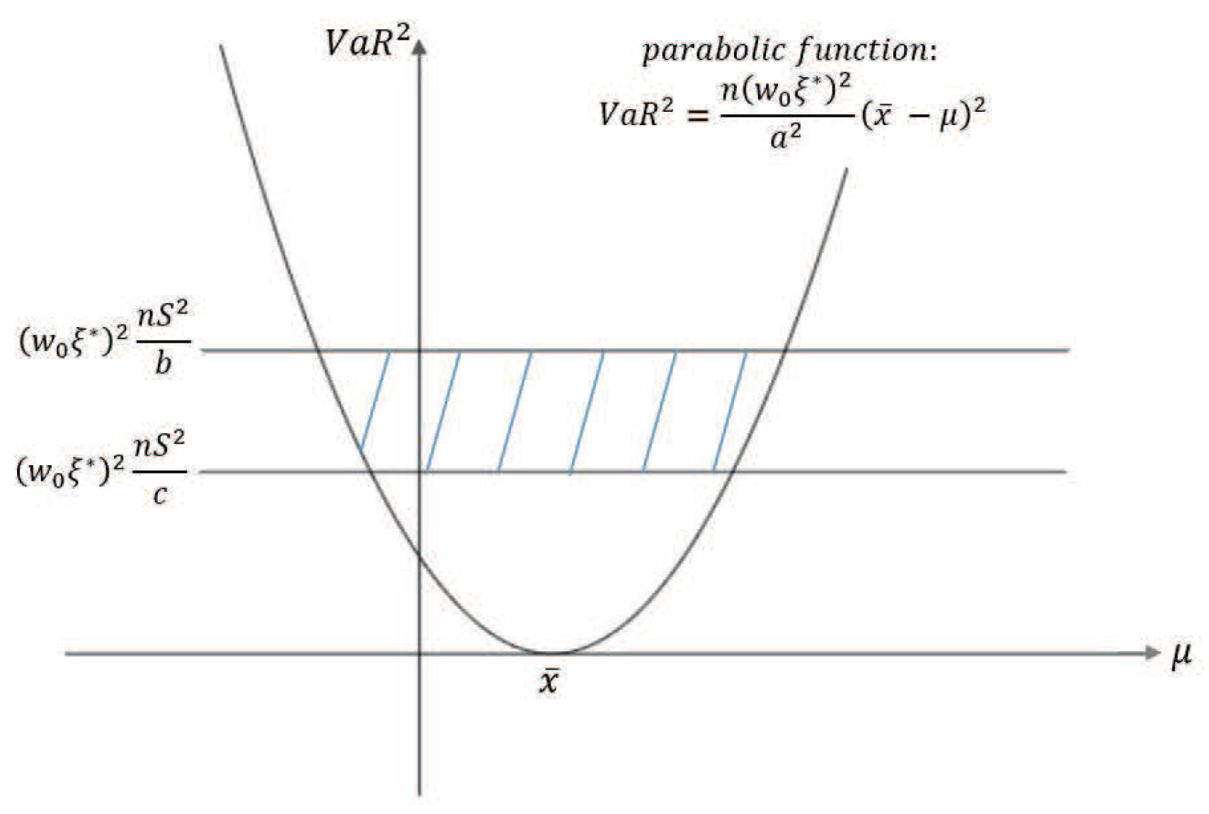
Assume that is a random vector, and are two index parameters, for given confidence level , one can define double-VaR of with respect to indexes as
whose figure is as Figure 2.
Remark 4.
Noticing the joint confidence region (see Figure 2) and combining with Markowitz’s portfolio theory, the right boundary of the banded region in Figure 2 can be regarded the dobule-VaR, , with . That is to say, one can have the following two basic understandings:
(1) For a given risk level , can be regarded as VaR in the sense of Markowitz’s portfolio with a given confidence level α;
(2) For a given benefit level , can also be regarded as VaR in the sense of Markowitz’s portfolio with a given confidence level α.
Clearly, we have
That is, there holds
where (or ) is the function value of distribution at the point b (or c) when the freedom is . Now we solve the unknowns and c by area minimization method.
The area of joint confidence region of can be calculated by double integrals:
Thus, after knowing we can solve the joint confidence region of by the following optimization problem:
Similarly, we can now solve the above optimization problem with fsolve function in MATLAB and get the unknowns , and c when the confidence level is respectively 99%, 95%, and 90% for . By the way, the value belonging to the area is also be gained as below.
At the same time, one can now solve the above optimization problem with fmincon function to solve constrained nonlinear minimization problem in MATLAB and get the unknowns , and c when the confidence level is respectively 99%,95%, and 90% for . Incidentally, the value belonging to the area can also be gained as below.
We can see the result of this model is similar to that under the area minimizing model; then there holds the following:
Theorem 1.
If the confidence level is not in the chart we can get the results by changing parameters in the program.
4. Empirical Analysis
4.1. Description of Sample Data
This subsection analyzes the sample data from the historical stock quotes in Merchants Bank of the Sohu securities network. The holding period is a month and there are a total of 40 pieces of data regarding closing prices in the observation period from 23 January 2009 to 27 April 2012. Now we want to predict at a given confidence level the mean and range of risks to China Merchants Bank stock yields at the end of May 2012, that is to solve the joint confidence region of .
Here we use the logarithmic gain: , where is the closing price of stock at time t. Thus, we can get 39 yields as below Table 7.
By AVERAGE and VAR function in Excel we can get the MLE: and of mean and variance are, respectively, and .
4.2. -Model
Effect between Ideal Point Method and the Method of the Smallest
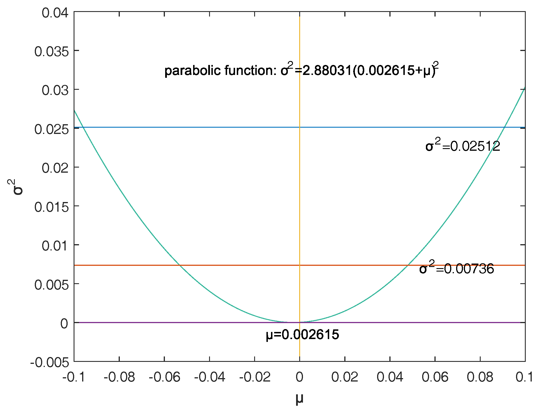
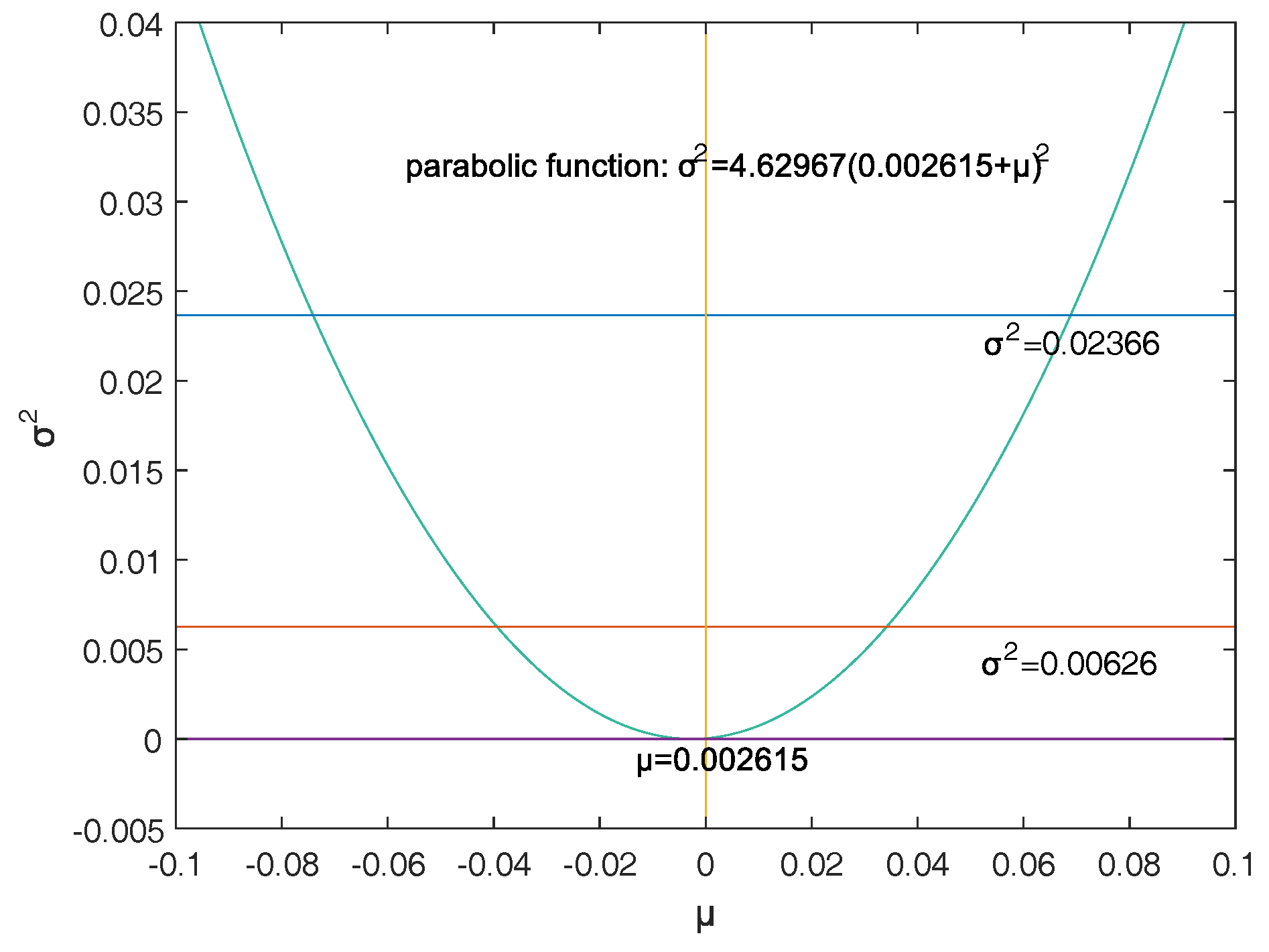
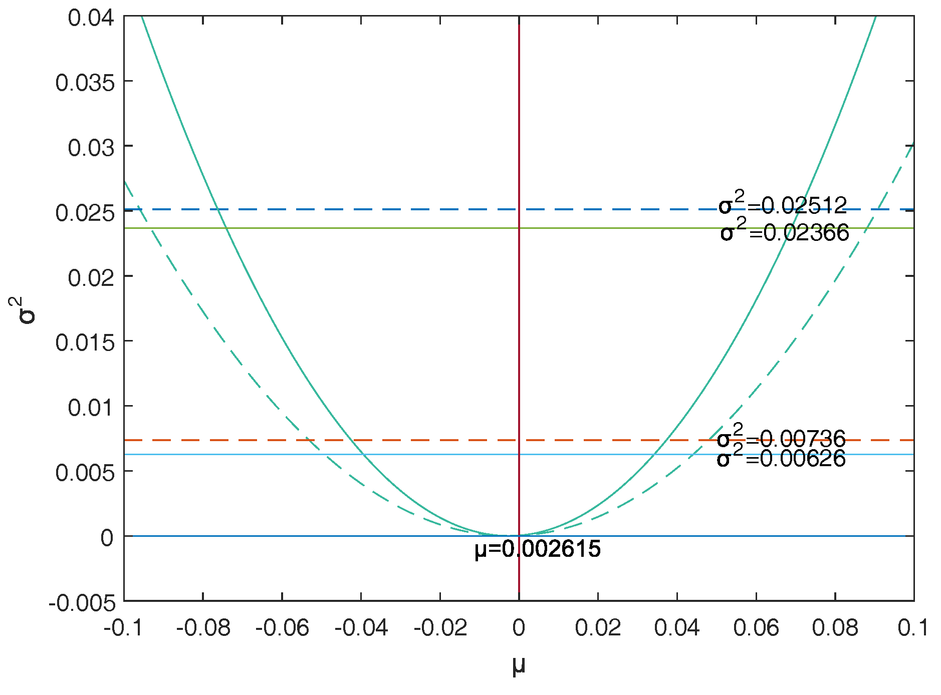
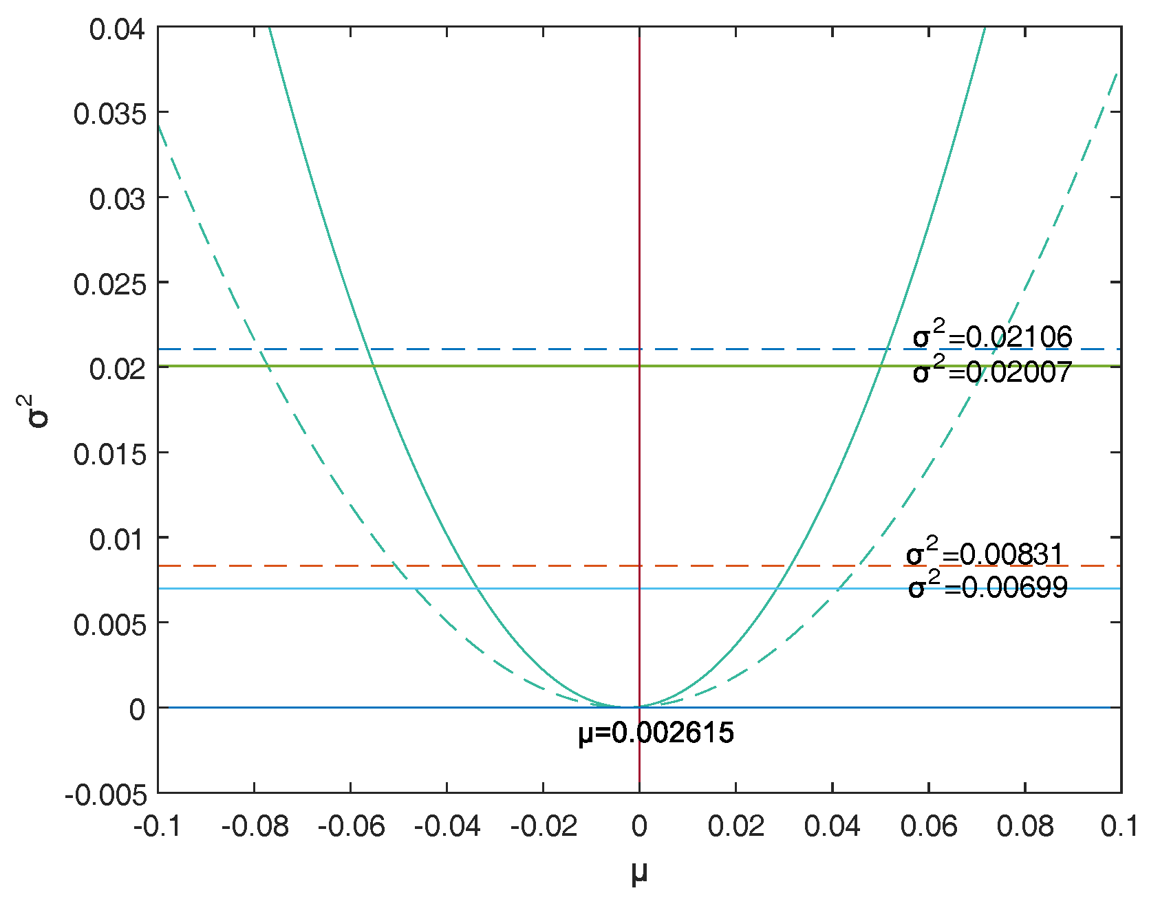
Now we respectively use ideal point method and area minimization method to solve the joint confidence region of at the given confidence level and make a contrast of the results from these two methods.
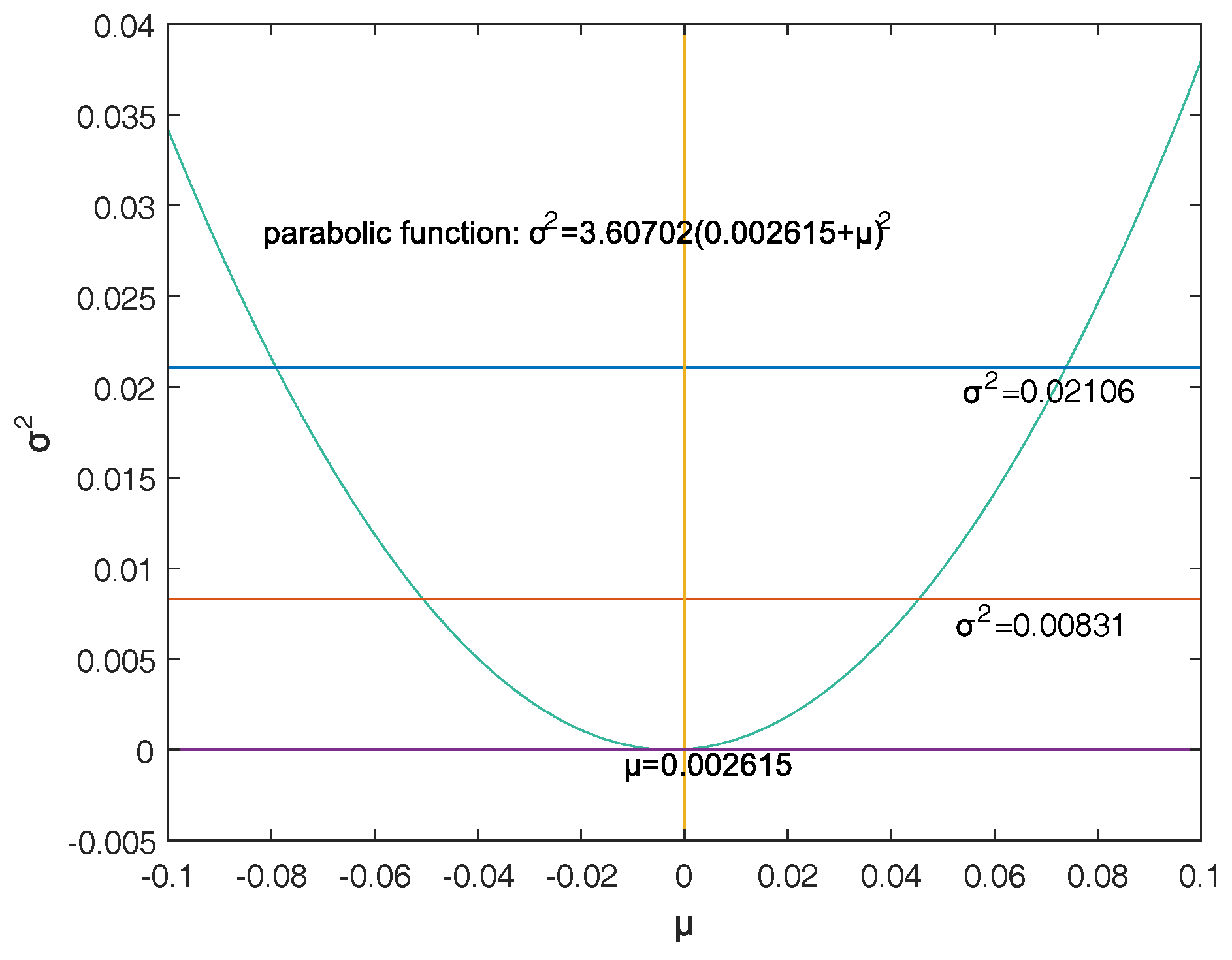
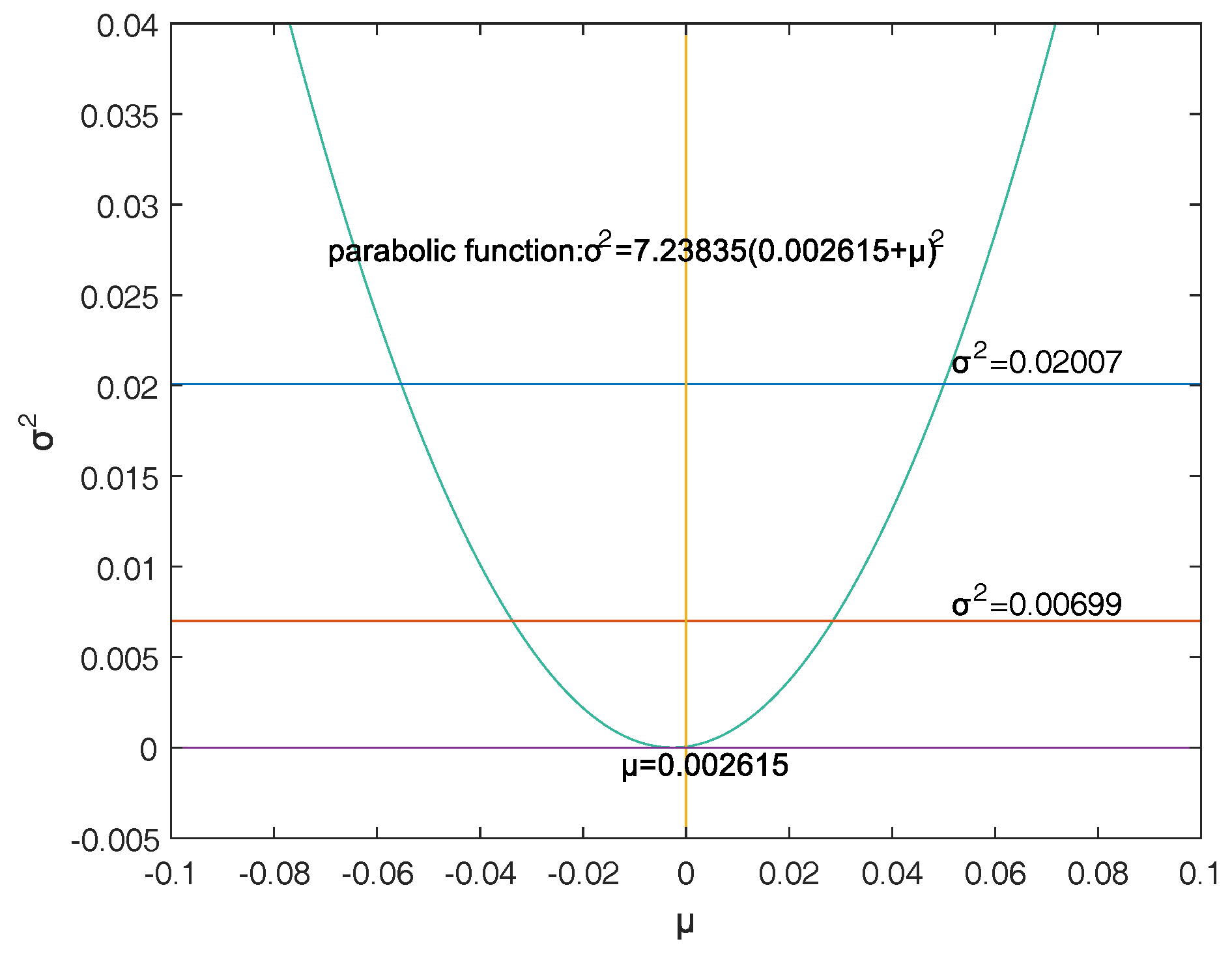
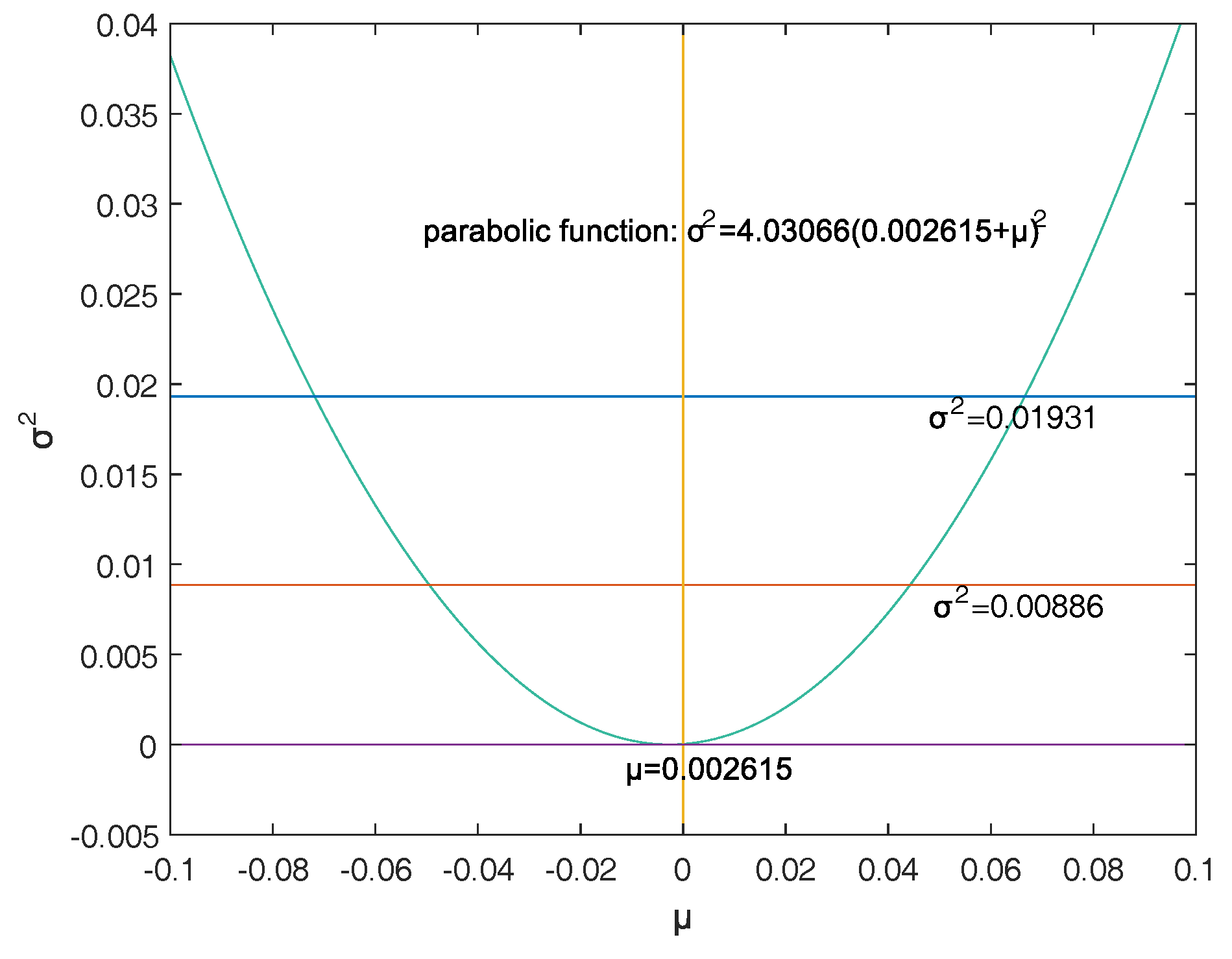
Put these values into the following formula and get the joint confidence region of as below
whose figure is the area enclosed by two horizontal lines and a parabola line
where the solid line is the result of area minimization method and the broken line is the result of ideal point method.
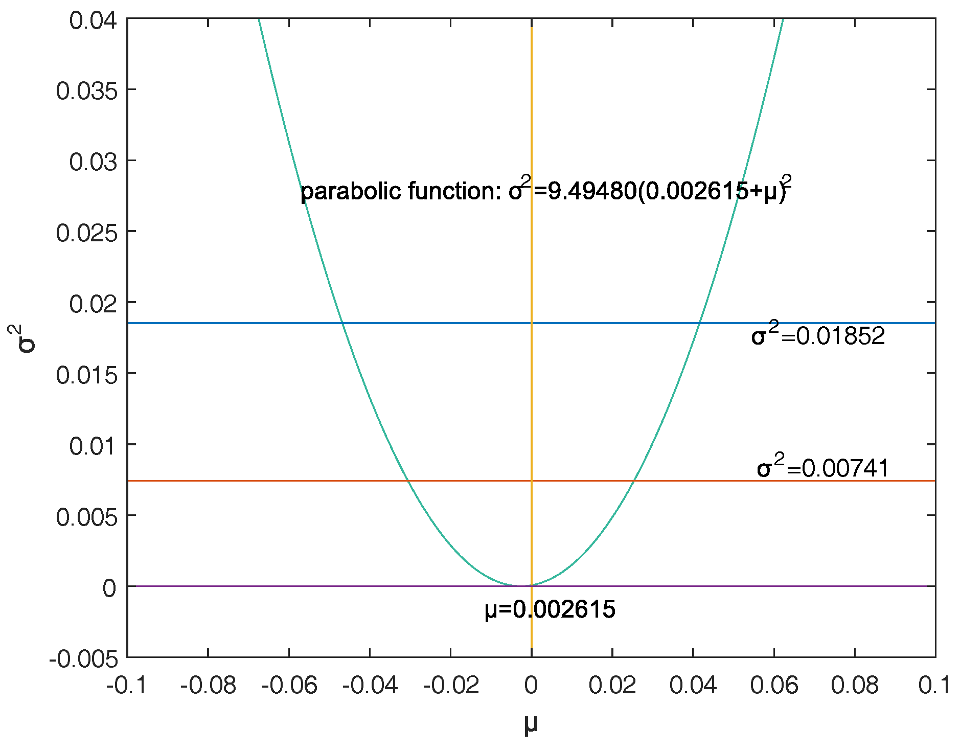
where the solid line is the result of area minimization method and the broken line is the result of ideal point method.
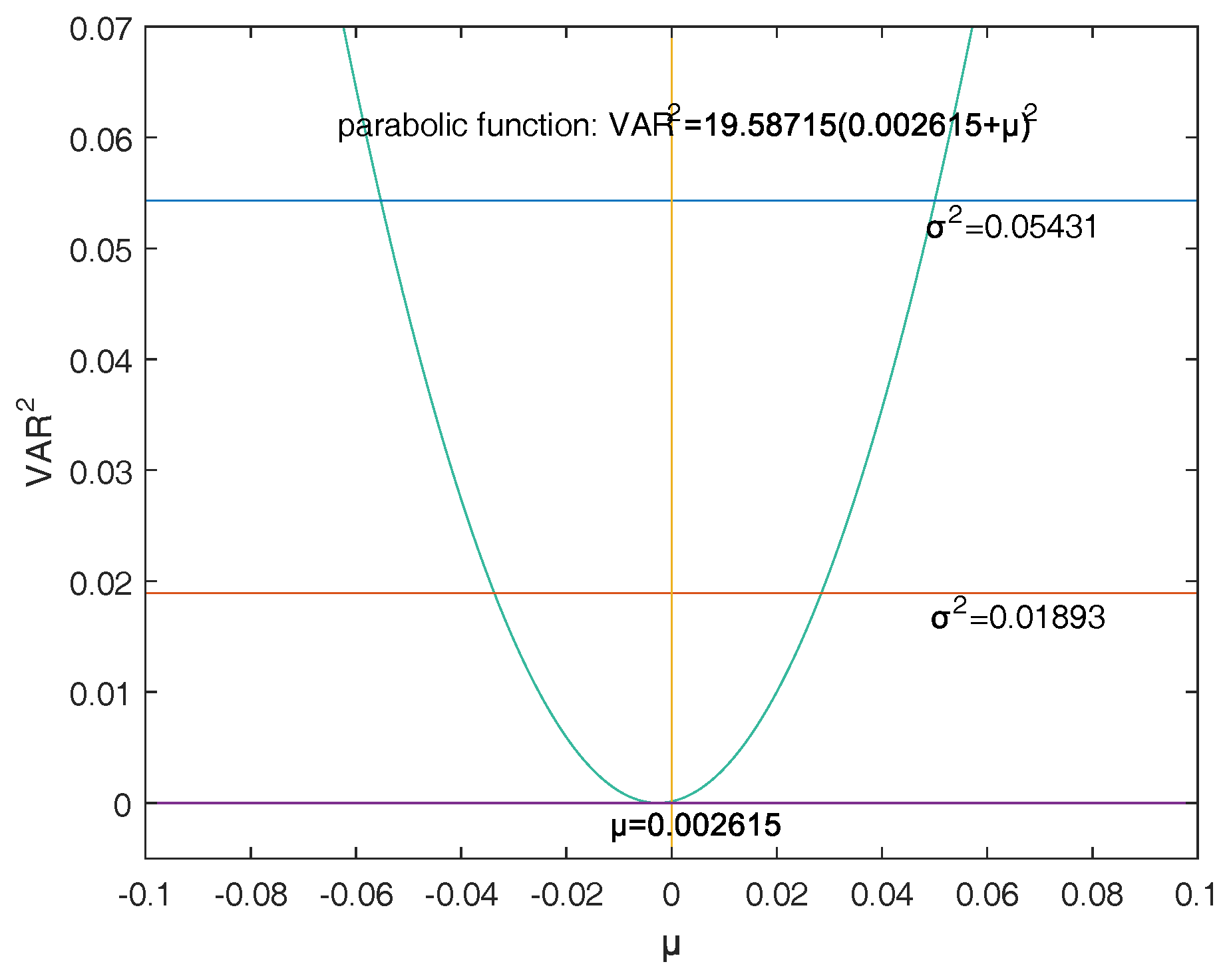
where the solid line is the result of area minimization method and the broken line is the result of ideal point method.
According to these results, we can know the area by area minimization method is smaller, so at a given confidence level area minimization method has a better effect to solve the joint confidence region of .
4.3. -Model
Suppose a customer buys shares of China Merchants Bank whose initial assets is and the confidence level of VaR is 95% that is . By Theorem 1 and the corresponding tables we have Table 10 as below.
Put these values into the following formula and get the joint confidence region of below
whose figure is the area enclosed by two horizontal lines and a parabola line.
(1) (confidence level is 99%) (Figure 12)
(2) (confidence level is 95%) (Figure 13)
(3) (confidence level is 90%) (Figure 14)
5. Conclusions
VaR is just a single indicator value to characterize risk, providing less information to the user, and the risk warning function is too thin. In practice, people often need to know both the benefits they may receive and the risks they are involved with. Therefore, this paper studies and constructs the double VaR according to the definition and research methods of VaR, expanding the one-dimensional single-risk monitoring indicator-VaR into a two-dimensional revenue-risk monitoring indicator.
This paper selects and as the models of the double-VaR. It shows the risk/maximum loss of an asset at a given time in the future and the area in which the revenue is located. Such indicators can better weigh the risk–return of assets, and deduce the joint confidence region of (or ) by virtue of the two-dimensional likelihood ratio method. Then, the ideal joint method and the area minimization method are used to solve the specific joint confidence domain, and the solution effect of the two methods is compared. The obtained area minimization method is more accurate and better. After the VaR is double-expanded, users can know more information and better evaluate assets and avoid certain financial risks.
In this paper, only the normal distribution is considered in terms of its own knowledge structure and time. In fact, the author has great interest in risk management in the case of market with fat tails and the probability of extreme events, which will have important practical significance. We will discuss this in the next article on VaR.
Author Contributions
All authors contributed equally and significantly to this paper. All authors read and approved the final manuscript.
Funding
This research was supported by the National Natural Science Foundation of China (No. 11871275; No. 11371194) and by a Grant-in-Aid for Science Research from Nanjing University of Science and Technology (2018M640485).
Conflicts of Interest
The authors declare no conflict of interest.
References
- Artzner, Philippe, Freddy Delbaen, Jean-Marc Eber, and David Heath. 1999. Coherent measures of risk. Mathematical Finance 9: 203–28. [Google Scholar] [CrossRef]
- Basak, Suleyman, and Alexander Shapiro. 2001. Value-at-Risk based risk management: Optimal policies and asset prices. Review of Financial Studies 14: 371–405. [Google Scholar] [CrossRef]
- Beder, Tanya Styblo. 1995. VAR: Seductive but dangerous. Financial Analysis Journal 51: 12–24. [Google Scholar] [CrossRef]
- Berkowitz, Jeremy. 1999. A Coherent Framework for Stress-Testing. Available online: http://www.federalreserve.gov/pubs/FEDS/1999/199929 (accessed on 28 February 2019).
- Berkowitz, Jeremy, and James O’Brien. 2002. How accurate are value-at-risk models at commercial banks. The Journal of Finance 57: 1093–111. [Google Scholar] [CrossRef]
- Chen, Huijun, and Tiefeng Jiang. 2017. A Study of Two High-dimensional Likelihood Ratio Tests under Alternative Hypotheses. Random Matrices: Theory and Applications 11: 1–21. [Google Scholar] [CrossRef]
- Chen, Rongda, Cong Li, Weijin Wang, and Ze Wang. 2014. Empirical analysis on future-cash arbitrage risk with portfolio VaR. Physica A: Statistical Mechanics and Its Applications 38: 210–16. [Google Scholar] [CrossRef]
- Cong, Chang, and Peibiao Zhao. 2018. Non-cash risk measure on nonconvex sets. Mathematics 6: 186. [Google Scholar] [CrossRef]
- Cong, Chang, and Peibiao Zhao. 2019. Non-cash Risk Measures on weak nonconvex sets. Forthcoming. [Google Scholar]
- Duffie, Darrell, and Jun Pan. 1997. An overview of value at risk. Journal of Derivatives 4: 7–49. [Google Scholar] [CrossRef]
- Engle, Robert F., and Simone Manganelli. 1999. CAViaR: Conditional Autoregressive Value at Risk by Regression Quantiles. Journal of Business and Economic Statistics 22: 367–81. [Google Scholar] [CrossRef]
- Hu, Ling. 2012. Dependence patterns across financial markets: A mixed copula approach. Applied Financial Economics 44: 2462–41. [Google Scholar] [CrossRef]
- Jackson, Patricia, David Maude, and William Perraudin. 1997. Bank capital and value-at-risk. Journal of Derivatives 4: 73–90. [Google Scholar] [CrossRef]
- Jorion, Philippe. 1996. Risk2: Measuring the risk in value at risk. Financial Analysis Journal 52: 47–56. [Google Scholar] [CrossRef]
- Jorion, Philippe. 2007. Value at Risk: The New Benchmark for Controlling Market Risk, 1st ed. Columbus: McGraw-Hill. [Google Scholar]
- Li, Zihe, Jinping Zhang, and Lanlan Feng. 2017. Analysis of Stock Risk Based on VaR and CVaR. Finance 7: 257–64. [Google Scholar] [CrossRef]
- Linsmeier, Thomas J., and Neil D. Pearson. 1996. Risk Measurement: An Introduction to Value at Risk. Available online: http://www.casact.net/education /specsem99frmgt/pearson2.pdf (accessed on 28 February 2019).
- Mausser, Helmut, and Dan Rosen. 1999. Beyond VaR from measuring risk to managing risk. ALGO Research Quarterly 1: 5–10. [Google Scholar]
- Pearson, Neil D. 2002. Risk Budgeting: Portfolio Problem Solving with Value-at-Risk, 1st ed. Hoboken: John Wiley and Sons. [Google Scholar]
- Potters, Marc, and Jean-Philippe Bouchaud. 1999. Worst Fluctuation Method for Fast Value-at-Risk Estimates. Available online: http://arxiv.org/pdf/cond-mat/9909245.pdf (accessed on 28 February 2019).[Green Version]
- Tang, Wanxiao, Fanchao Zhou, and Peibiao Zhao. 2018. Harnack inequality and no-arbitrage analysis. Symmetry 10: 517. [Google Scholar] [CrossRef]
- Taylor, Nick, Dick Van Dijk, Philip Hans Franses, and Andre Lucas. 2000. SETS, arbitrage activity, and stock price dynamics. Journal of Banking and Finance 24: 1289–306. [Google Scholar] [CrossRef]
- Wang, Tan. 1999. A Class of Dynamic Risk Measures. Available online: http://web.cenet.org.cn/upfile/57263.pdf (accessed on 28 February 2019).
- Ze-To, Samuel Yau Man. 2013. Estimating value-at-risk under a Heath-Jarrow-Morton framework with jump. Applied Economics 38: 1102–248. [Google Scholar] [CrossRef]
Figure 1.
The joint confidence region of .

Figure 2.
The joint confidence region of .

Figure 3.
The joint confidence region of by ideal point method.

Figure 4.
The joint confidence region of by area minimization method.

Figure 5.
The contrast of two methods.

Figure 6.
The joint confidence region of by ideal point method.

Figure 7.
The joint confidence region of by area minimization method.

Figure 8.
The contrast of two methods.

Figure 9.
The joint confidence region of by ideal point method.

Figure 10.
The joint confidence region of by area minimization method.

Figure 11.
The contrast of two methods.

Figure 12.
The joint confidence region of when .

Figure 13.
The joint confidence region of when .

Figure 14.
The joint confidence region of when .


Table 1.
Ideal point method (confidence level is 99% and 95%).
| Ideal Point (Confidence Level: 99%) | Ideal Point (Confidence Level: 95%) | |||||||
|---|---|---|---|---|---|---|---|---|
| n | a | b | c | zz | a | b | c | zz |
| 31 | 3.6185 | 13.0228 | 52.5124 | 0.0675 | 3.2248 | 15.9692 | 45.8943 | 0.0402 |
| 32 | 3.6284 | 13.6810 | 53.8337 | 0.0625 | 3.2340 | 16.7118 | 47.1456 | 0.0373 |
| 33 | 3.6373 | 14.3476 | 55.1539 | 0.0580 | 3.2427 | 17.4595 | 48.3940 | 0.0348 |
| 34 | 3.6454 | 15.0216 | 56.4719 | 0.0540 | 3.2510 | 18.2119 | 49.6392 | 0.0325 |
| 35 | 3.6529 | 15.7018 | 57.7869 | 0.0504 | 3.2590 | 18.9685 | 50.8812 | 0.0305 |
| 36 | 3.6601 | 16.3877 | 59.0984 | 0.0471 | 3.2666 | 19.7289 | 52.1197 | 0.0286 |
| 37 | 3.6668 | 17.0785 | 60.4060 | 0.0441 | 3.2740 | 20.4929 | 53.3550 | 0.0269 |
| 38 | 3.6734 | 17.7739 | 61.7097 | 0.0414 | 3.2812 | 21.2604 | 54.5870 | 0.0253 |
| 39 | 3.6797 | 18.4736 | 63.0094 | 0.0390 | 3.2882 | 22.0311 | 55.8159 | 0.0239 |
| 40 | 3.6858 | 19.1774 | 64.3053 | 0.0367 | 3.2949 | 22.8048 | 57.0417 | 0.0226 |
| 41 | 3.6918 | 19.8851 | 65.5974 | 0.0347 | 3.3015 | 23.5816 | 58.2646 | 0.0214 |
| 42 | 3.6975 | 20.5965 | 66.8858 | 0.0328 | 3.3079 | 24.3612 | 59.4847 | 0.0203 |
| 43 | 3.7032 | 21.3115 | 68.1707 | 0.0311 | 3.3141 | 25.1435 | 60.7021 | 0.0193 |
| 44 | 3.7086 | 22.0299 | 69.4522 | 0.0295 | 3.3202 | 25.9285 | 61.9168 | 0.0183 |
| 45 | 3.7140 | 22.7516 | 70.7304 | 0.0280 | 3.3261 | 26.7160 | 63.1291 | 0.0175 |
Table 2.
Ideal point method (confidence level is 90%).
| n | a | b | c | zz |
|---|---|---|---|---|
| 31 | 3.0444 | 17.6622 | 42.7490 | 0.0301 |
| 32 | 3.0539 | 18.4464 | 43.9610 | 0.0281 |
| 33 | 3.0629 | 19.2348 | 45.1702 | 0.0262 |
| 34 | 3.0715 | 20.0270 | 46.3766 | 0.0245 |
| 35 | 3.0799 | 20.8225 | 47.5800 | 0.0230 |
| 36 | 3.0879 | 21.6213 | 48.7805 | 0.0217 |
| 37 | 3.0957 | 22.4231 | 49.9782 | 0.0204 |
| 38 | 3.1033 | 23.2277 | 51.1732 | 0.0192 |
| 39 | 3.1106 | 24.0351 | 52.3654 | 0.0182 |
| 40 | 3.1178 | 24.8451 | 53.5552 | 0.0172 |
| 41 | 3.1247 | 25.6575 | 54.7424 | 0.0163 |
| 42 | 3.1314 | 26.4724 | 55.9273 | 0.0155 |
| 43 | 3.1380 | 27.2895 | 57.1099 | 0.0147 |
| 44 | 3.1444 | 28.1089 | 58.2902 | 0.0140 |
| 45 | 3.1507 | 28.9304 | 59.4685 | 0.0134 |
Table 3.
Minimizing area method (confidence level is 99% and 95%).
| Min-Area (Confidence Level: 99%) | Min-Area (Confidence Level: 95%) | |||||||
|---|---|---|---|---|---|---|---|---|
| n | a | b | c | zz | a | b | c | zz |
| 31 | 2.9246 | 14.1512 | 63.8981 | 0.0492 | 2.3414 | 17.1303 | 56.5295 | 0.0275 |
| 32 | 2.9215 | 14.8181 | 65.1849 | 0.0457 | 2.3384 | 17.8670 | 57.7614 | 0.0256 |
| 33 | 2.9185 | 15.4917 | 66.4687 | 0.0425 | 2.3356 | 18.6088 | 58.9919 | 0.0239 |
| 34 | 2.9152 | 16.1680 | 67.7464 | 0.0396 | 2.3328 | 19.3513 | 60.2205 | 0.0224 |
| 35 | 2.9123 | 16.8527 | 69.0219 | 0.0370 | 2.3301 | 20.0984 | 61.4518 | 0.0210 |
| 36 | 2.9100 | 17.5339 | 70.3055 | 0.0347 | 2.3279 | 20.8511 | 62.6723 | 0.0198 |
| 37 | 2.9070 | 18.2239 | 71.5778 | 0.0326 | 2.3255 | 21.6032 | 63.8980 | 0.0186 |
| 38 | 2.9050 | 18.9163 | 72.8532 | 0.0306 | 2.3233 | 22.3595 | 65.1167 | 0.0176 |
| 39 | 2.9024 | 19.6137 | 74.1233 | 0.0289 | 2.3212 | 23.1191 | 66.3364 | 0.0166 |
| 40 | 2.9005 | 20.3139 | 75.3969 | 0.0272 | 2.3192 | 23.8815 | 67.5544 | 0.0157 |
| 41 | 2.8969 | 21.0252 | 76.6403 | 0.0257 | 2.3175 | 24.6494 | 68.7771 | 0.0149 |
| 42 | 2.8968 | 21.7419 | 77.9333 | 0.0244 | 2.3155 | 25.4145 | 69.9847 | 0.0141 |
| 43 | 2.8946 | 22.4362 | 79.1883 | 0.0231 | 2.3137 | 26.1851 | 71.2024 | 0.0134 |
| 44 | 2.8902 | 23.1570 | 80.4262 | 0.0219 | 2.3121 | 26.9580 | 72.4080 | 0.0128 |
| 45 | 2.8918 | 23.8752 | 81.7268 | 0.0209 | 2.3105 | 27.7325 | 73.6185 | 0.0122 |
Table 4.
Minimizing area point method (confidence level is 90%).
| n | a | b | c | zz |
|---|---|---|---|---|
| 31 | 2.0457 | 18.7961 | 53.0159 | 0.0198 |
| 32 | 2.0428 | 19.5671 | 54.2198 | 0.0185 |
| 33 | 2.0401 | 20.3418 | 55.4228 | 0.0173 |
| 34 | 2.0375 | 21.1193 | 56.6243 | 0.0162 |
| 35 | 2.0351 | 21.9005 | 57.8240 | 0.0152 |
| 36 | 2.0328 | 22.6834 | 59.0225 | 0.0143 |
| 37 | 2.0307 | 23.4694 | 60.2189 | 0.0135 |
| 38 | 2.0286 | 24.2587 | 61.4147 | 0.0128 |
| 39 | 2.0267 | 25.0498 | 62.6071 | 0.0121 |
| 40 | 2.0248 | 25.8426 | 63.7978 | 0.0114 |
| 41 | 2.0230 | 26.6392 | 64.9906 | 0.0109 |
| 42 | 2.0213 | 27.4365 | 66.1760 | 0.0103 |
| 43 | 2.0197 | 28.2368 | 67.3628 | 0.0098 |
| 44 | 2.0182 | 29.0392 | 68.5481 | 0.0093 |
| 45 | 2.0167 | 29.8436 | 69.7319 | 0.0089 |
Table 5.
Minimizing area method (confidence level is 99% and 95%).
| Min-Area (Confidence Level: 99%) | Min-Area (Confidence Level: 95%) | |||||||
|---|---|---|---|---|---|---|---|---|
| n | a | b | c | zz | a | b | c | zz |
| 46 | 3.0064 | 21.7720 | 78.4073 | 0.0253 | 2.3977 | 27.4369 | 72.2900 | 0.0128 |
| 47 | 3.0024 | 22.4891 | 79.6858 | 0.0239 | 2.3941 | 28.2136 | 73.5112 | 0.0122 |
| 48 | 2.9983 | 23.2131 | 80.9560 | 0.0227 | 2.3910 | 28.9950 | 74.7342 | 0.0116 |
| 49 | 2.9944 | 23.9403 | 82.2217 | 0.0215 | 2.3880 | 29.7792 | 75.9545 | 0.0111 |
| 50 | 2.9882 | 24.6870 | 83.4624 | 0.0204 | 2.3853 | 30.5680 | 77.1736 | 0.0106 |
| 60 | 3.1182 | 30.7638 | 87.6602 | 0.0145 | 2.3613 | 38.5214 | 89.2508 | 0.0071 |
| 70 | 2.9378 | 39.7032 | 108.3873 | 0.0091 | 2.3443 | 46.6338 | 101.1698 | 0.0051 |
| 80 | 3.2519 | 34.5137 | 108.8108 | 0.0132 | 2.3312 | 54.8651 | 112.9622 | 0.0038 |
| 90 | 1.1088 | 24.1613 | 27.8069 | 0.0018 | 1.0750 | 24.1328 | 27.6881 | 0.0017 |
| 100 | 5.5409 | 23.9661 | 26.2147 | 0.0059 | 5.5450 | 23.9705 | 26.2556 | 0.0060 |
Table 6.
Minimizing area point method (confidence level is 90%).
| n | a | b | c | zz |
|---|---|---|---|---|
| 46 | 2.0912 | 30.2984 | 69.2514 | 0.0089 |
| 47 | 2.0884 | 31.1074 | 70.4505 | 0.0085 |
| 48 | 2.0857 | 31.9191 | 71.6481 | 0.0081 |
| 49 | 2.0831 | 32.7310 | 72.8427 | 0.0078 |
| 50 | 2.0806 | 33.5453 | 74.0353 | 0.0074 |
| 60 | 2.0598 | 41.7726 | 85.8687 | 0.0050 |
| 70 | 2.0447 | 50.1308 | 97.5564 | 0.0036 |
| 80 | 2.0333 | 58.5941 | 109.1282 | 0.0027 |
| 90 | 1.0479 | 24.0945 | 27.5455 | 0.0016 |
| 100 | 5.5482 | 23.9796 | 26.3103 | 0.0061 |
Table 7.
Sample data year and month closing price yield.
| Sample Data | Sample Data | Sample Data | ||||||
|---|---|---|---|---|---|---|---|---|
| Y-M | price | yield | Y-M | price | yield | Y-M | price | yield |
| 0901 | 13.51 | - | 1001 | 15.17 | −0.173826 | 1101 | 12.63 | −0.014151 |
| 0902 | 14.27 | 0.054729 | 1002 | 15.90 | 0.046999 | 1102 | 12.87 | 0.018824 |
| 0903 | 15.93 | 0.110045 | 1003 | 16.28 | 0.023618 | 1103 | 14.09 | 0.090566 |
| 0904 | 15.50 | −0.027364 | 1004 | 14.27 | −0.131778 | 1104 | 14.46 | 0.025921 |
| 0905 | 16.86 | 0.084104 | 1005 | 13.23 | −0.075672 | 1105 | 13.91 | −0.038778 |
| 0906 | 22.41 | 0.284563 | 1006 | 13.01 | −0.016769 | 1106 | 13.02 | −0.066121 |
| 0907 | 19.64 | −0.131939 | 1007 | 14.52 | 0.109809 | 1107 | 12.35 | −0.052831 |
| 0908 | 13.63 | −0.365295 | 1008 | 13.54 | −0.069879 | 1108 | 11.85 | −0.041328 |
| 0909 | 14.78 | 0.081002 | 1009 | 12.95 | −0.044552 | 1109 | 11.06 | −0.068993 |
| 0910 | 17.77 | 0.184237 | 1010 | 14.57 | 0.117869 | 1110 | 12.10 | 0.089870 |
| 0911 | 17.29 | −0.027383 | 1011 | 13.05 | −0.110176 | 1111 | 11.21 | −0.076399 |
| 0912 | 18.05 | 0.043017 | 1012 | 12.81 | −0.018562 | 1112 | 11.87 | 0.057208 |
| - | - | - | - | - | - | 1201 | 12.65 | 0.063643 |
| - | - | - | - | - | - | 1202 | 12.87 | 0.017242 |
| - | - | - | - | - | - | 1203 | 11.90 | −0.078361 |
| - | - | - | - | - | - | 1204 | 12.20 | 0.024898 |
Table 8.
(confidence level 99% and 95%).
| Confidence Level 99% | Confidence Level 95% | |||||||
|---|---|---|---|---|---|---|---|---|
| Method | a | b | c | zz | a | b | c | zz |
| ideal point | 3.6797 | 18.4736 | 63.0094 | 0.0390 | 3.2882 | 22.0311 | 55.8159 | 0.0239 |
| Min-area | 2.9024 | 19.6137 | 74.1233 | 0.0289 | 2.3212 | 23.1191 | 66.3364 | 0.0166 |
Table 9.
(confidence level is 90%).
| Method | a | b | c | zz |
|---|---|---|---|---|
| ideal point | 3.1106 | 24.0351 | 52.3654 | 0.0182 |
| Min-area | 2.0267 | 25.0498 | 62.6071 | 0.0121 |
Table 10.
.
| a | b | c | zz | |
|---|---|---|---|---|
| 1% | 2.9024 | 19.6137 | 74.1233 | 0.0289 |
| 5% | 2.3212 | 23.1191 | 66.3364 | 0.0166 |
| 10% | 2.0267 | 25.0498 | 62.6071 | 0.0121 |
© 2019 by the authors. Licensee MDPI, Basel, Switzerland. This article is an open access article distributed under the terms and conditions of the Creative Commons Attribution (CC BY) license (http://creativecommons.org/licenses/by/4.0/).
Share and Cite
MDPI and ACS Style
Zhang, W.; Zhang, S.; Zhao, P. On Double Value at Risk. Risks 2019, 7, 31. https://doi.org/10.3390/risks7010031
AMA Style
Zhang W, Zhang S, Zhao P. On Double Value at Risk. Risks. 2019; 7(1):31. https://doi.org/10.3390/risks7010031
Chicago/Turabian StyleZhang, Wanbing, Sisi Zhang, and Peibiao Zhao. 2019. "On Double Value at Risk" Risks 7, no. 1: 31. https://doi.org/10.3390/risks7010031
Note that from the first issue of 2016, this journal uses article numbers instead of page numbers. See further details here.