Multiple Time Series Forecasting Using Quasi-Randomized Functional Link Neural Networks


1
ISFA, Laboratoire SAF, Université Claude Bernard Lyon I, 69100 Villeurbanne, France
2
Laboratoire IRMA, Université de Strasbourg, 67081 Strasbourg, France
*
Author to whom correspondence should be addressed.
Risks 2018, 6(1), 22; https://doi.org/10.3390/risks6010022
Submission received: 3 January 2018
/
Revised: 16 February 2018
/
Accepted: 26 February 2018
/
Published: 12 March 2018
Abstract
:We are interested in obtaining forecasts for multiple time series, by taking into account the potential nonlinear relationships between their observations. For this purpose, we use a specific type of regression model on an augmented dataset of lagged time series. Our model is inspired by dynamic regression models (Pankratz 2012), with the response variable’s lags included as predictors, and is known as Random Vector Functional Link (RVFL) neural networks. The RVFL neural networks have been successfully applied in the past, to solving regression and classification problems. The novelty of our approach is to apply an RVFL model to multivariate time series, under two separate regularization constraints on the regression parameters.
1. Introduction
In this paper, we are interested in obtaining forecasts for multiple time series, by taking into account the potential nonlinear relationships between their observations. This type of problem has been tackled recently by Exterkate et al. (2016), who applied kernel regularized least squares to a set of macroeconomic time series. The Long Short-Term Memory neural networks (LSTM) architectures (introduced by Hochreiter and Schmidhuber (1997)) are another family of models, which are currently widely used for this purpose. As a basis for our model, we will use (quasi-)randomized neural networks known as Random Vector Functional Link neural networks (RVFL networks hereafter).
The forecasting method described in this paper, provides useful inputs for Insurance Quantitative Risk Management models; the interested reader can refer to Bonnin et al. (2015) for an example.
To the best of our knowledge, randomized neural networks were introduced by Schmidt et al. (1992), and the RVFL networks were introduced by Pao et al. (1994). An early approach for multivariate time series forecasting using neural networks is described in Chakraborty et al. (1992). They applied a back propagation algorithm from Rumelhart et al. (1988) to trivariate time series, and found that the combined training of the series gave better forecasts than a separate training of each individual series. The novelty of the approach described in this paper is to derive an RVFL model for multiple time series, under two separate regularization constraints on the parameters, as it will be described in detail in Section 2.3.
RVFL networks are multilayer feedforward neural networks, in which there is a direct link between the predictors and the output variable, aiming at capturing the linear relationships. In addition to the direct link, there are new features: the hidden nodes (the dataset is augmented), that help to capture the nonlinear relationships between the time series. These new features are obtained by random simulation over a given interval. More details on the direct link and the hidden nodes will be provided in the next section.
The RVFL networks have been successfully applied to solving different types of classification and regression problems, see for example Dehuri and Cho (2010). More specifically, they have been applied to univariate time series forecasting by Ren et al. (2016). A comprehensive survey can be found in Zhang and Suganthan (2016), where a large number of model specifications are tested on classification problems, including changing the range of hidden layer’s randomization.
Here, we will use RVFL networks with one hidden layer. Furthermore, instead of relying on fully randomized nodes, we will use sequences of deterministic quasi-random numbers. Indeed, with fully randomized nodes, the model fits obtained are dependent on the choice of a simulation seed. Typically, a different fitting solution would be obtained for each seed.
In our various numerical examples from Section 3, we will apply the RVFL networks to forecasting trivariate time series, notably (but not only) in a Dynamic Nelson Siegel (DNS) framework (see Nelson and Siegel 1987; Diebold and Li 2006). We will obtain point forecasts and predictive distributions for the series, and see that in this RVFL framework, one (or more) variable(s) can be stressed, and influence the others. More precisely, about this last point, it means that it is possible, as in dynamic regression models (Pankratz 2012) to assign a specific future value to one regressor, and obtain forecasts of the remaining variables. Another advantage of the model described here is its ability to integrate multiple other exogenous variables, without overfitting in-sample data.
2. Description of the Model
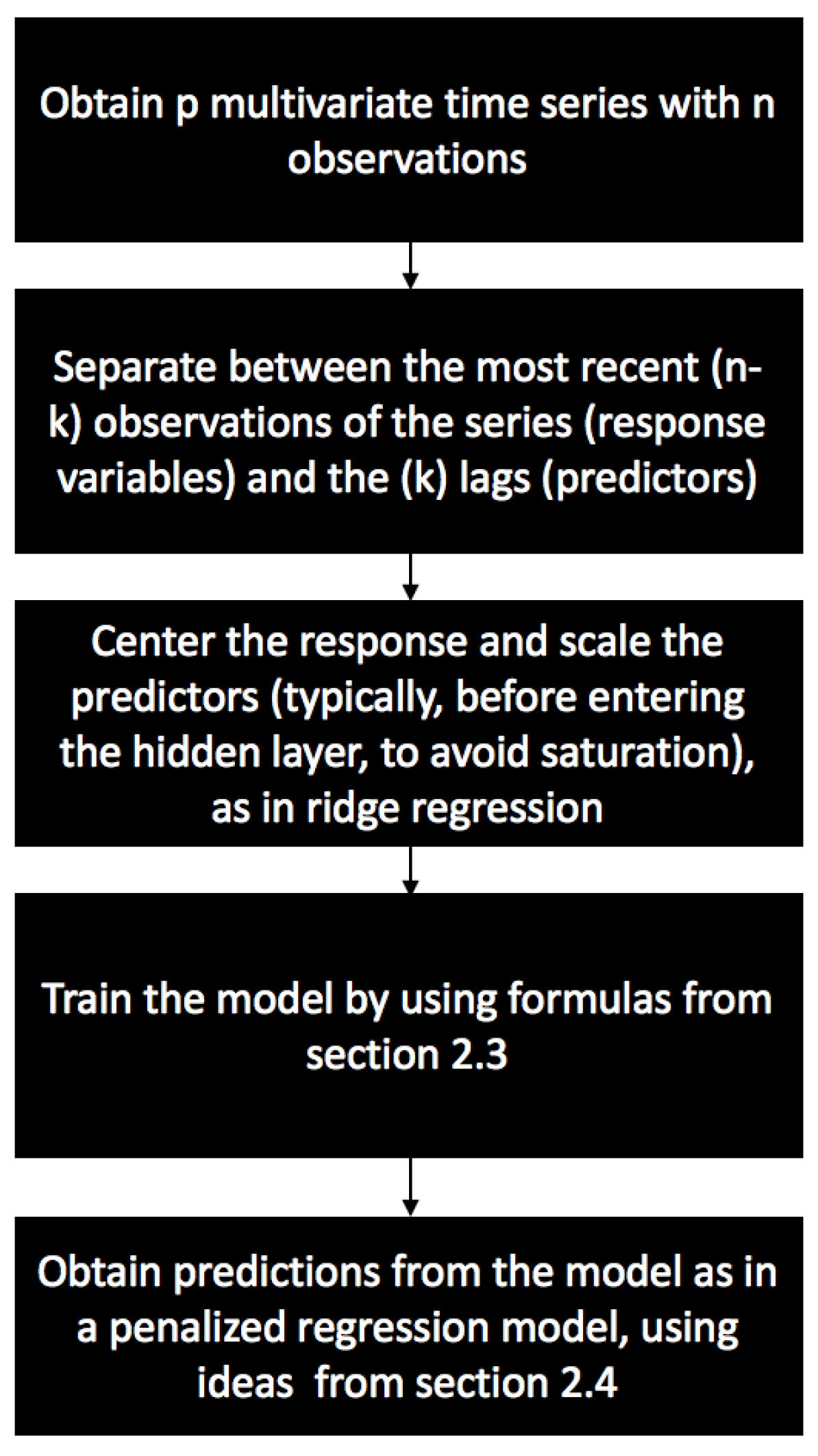
The general procedure for obtaining the model’s optimal parameters and predictions is summarized in Figure 1.
This procedure is described in detail in the next sections, especially in Section 2.3 and Section 2.4.
2.1. On a Single Layer RVFL Network
We rely on single layer feed forward neural networks (SLFN). Considering that an output variable is to be explained by a set of observed predictors , , the RVFL networks we will use to explain y can be described for as:
g is called activation function, L is the number of nodes in the hidden layer, are elements of the hidden layer, and the parameters and are to be learned from the observed data . The ’s are the residual differences between the output variable values and the RVFL model.
This type of model can be seen as one explaining , by finding a compromise between linear and potentially non-linear effects of the original predictors and transformed predictors
on the response. Common choices for function g in neural networks regression are the sigmoïd activation function
the hyperbolic tangent function,
or the Rectified Linear Units, known as ReLU
The main differences between the RVFL framework and a classical SLFN framework are:
- The inclusion of a linear dependence between the output variable and the predictors: the direct link, .
- The elements of the hidden layer are typically not trained, but randomly and uniformly chosen on a given interval. Different ranges for these elements of the hidden layer are tested in (Zhang and Suganthan 2016).
Solving for the optimal parameters ’s and ’s can be done by applying directy a least squares regression of y on the set of observed and transformed predictors. But since these input predictors are likely to be highly correlated—especially in our setting, with time series data—we do not search each of these parameters on the entire line, but in restricted regions where we have:
and
for . That is, applying some kind of Tikhonov regularization or ridge regression model (Hoerl and Kennard 1970) of y on the set of observed and transformed predictors. Having two constraints instead of one allows for more flexibility in the covariance structure between the predictors and the output, with ’s and ’s moving in separate balls. For these constraints to be applicable, the input variables will need to be standardized, so as to be expressed on the same scales, and the response variable will be centered.
Imposing these restrictions to the model’s parameters increases their interpretability—by reducing their variance—at the expense of a slight increase in in-sample bias. It also prevents the model from overfitting the data as in ridge regression (Hoerl and Kennard 1970). One of the advantages of RVFL networks is that they are relatively fast to train, due to the availability of closed-form formulas for the model’s parameters, as it will be presented in the next section.
On the other hand, RVFL networks incorporate some randomness in the hidden layer, which makes each model relatively dependent on the choice of a simulation seed. Each seed would indeed produce a different set of parameters ’s and ’s for the model. For that reason, we will also use sequences of deterministic quasi-random numbers in the hidden layer. The elements of the hidden layer are taken from a quasi-random (deterministic) sobol sequence on , which is shifted in such a way that they belong to .
Sobol sequences are part of quasi-random numbers, which are also called low discrepancy sequences. As described intuitively in Boyle and Tan (1997), the discrepancy of a sequence of N points in a subcube is defined as:
where is the volume of V. It describes how well the points are dispersed within V. The idea is to have points which are more or less equidispersed in V. Joe and Kuo (2008) describe the generation of the term, component () of a Sobol sequence. The generation starts with obtaining the binary representation of i. That is, obtaining i as:
For example, can be expressed as in binary representation. Then, by using the sequence of bits describing i in base 2, we can obtain as:
where ⊕ is a bitwise exclusive-or operation, and the numbers are called the direction numbers, defined for as:
A few details on Equation (2):
- The bitwise exclusive-or operation ⊕ applied to two integers p and returns 1 if and only if one of the two (but not both) inputs is equal to 1. Otherwise, is equal to 0.
- The second term of the equation relies on primitive polynomials of degree , with coefficients taken in :
- The terms are obtained recursively, with the initial values chosen freely, under the condition that is odd and less than .
A more complete treatment of low discrepancy sequences can be found in Niederreiter (1992). In addition, an example with , , is given in Joe and Kuo (2008).
2.2. Applying RVFL Networks to Multivariate Time Series Forecasting
We consider time series , observed at discrete dates. We are interested in obtaining simultaneous forecasts of the p time series at time , , by allowing each of the p variables to be influenced by the others (in the spirit of VAR models, see Lütkepohl 2005).
For this purpose, we use lags of each of the observed p time series. The output variables to be explained are:
for . Where is the most contemporaneous observed value of the j-th time series, and was observed k dates earlier in time for . These output variables are stored in a matrix:
and the predictors are stored in a matrix:
where consists in p blocks of k lags, for each one of the observed p time series. For example, the block of , for contains in columns:
with . It is also possible to add other regressors, such as dummy variables, indicators of special events, but for clarity, we consider only the inclusion of lags.
As described in the previous section, an additional layer of transformed predictors is added to , in order to capture the potentially non-linear interactions between the predictors and the output variable. Adding the transformed predictors to the original ones leads to a new matrix of predictors with dimensions , where L is the number of nodes in the hidden layer. We are then looking for simultaneous predictions
for , and . This is a multi-task learning problem (see Caruana 1998), in which the output variables will all share the same set of predictors.
For example, we have time series and observed at dates , with lags, and nodes in the hidden layer. In this case, the response variables are stored in:
The predictors are stored in:
And the coefficients in the hidden layer are:
2.3. Solving for ’s and ’s
We let y be the column (out of p) of the response matrix , and be the matrix of transformed predictors obtained from by the hidden layer described at the beginning of Section 2.1. We also denote the set of regression parameters associated with this time series, as:
and
for ; . Solving for the regression parameters for the time series, under the constraints
and
for , leads to minimizing a penalized residual sum of squares. Hence, for vectors and containing the regression parameters, we obtain the Lagrangian:
where and are Lagrange multipliers. Taking the first derivatives of relative to and leads to:
where is the identity matrix with dimensions and equivalently
where is the identity matrix with dimensions . And setting these first derivatives to 0 leads to:
That is:
Now, if we denote:
and . Then, using the algorithm described in Cormen (2009) for blockwise matrix inversion, we obtain:
where and are the Moore-Penrose pseudo-inverse (Penrose 1955) of matrixes S and B. Hence for each column y of , we have the solutions:
And the whole set of parameters, for all the p observed time series is given by:
The objective function to be minimized (the least squares) is convex, and so is the set of feasible solutions. The solutions and found here are hence global minima.
2.4. h-Steps Ahead Forecasts and Use of Dynamic Regression
Having obtained the optimal set of parameters and as described in the previous section, a new set of predictors is constructed by using the former output variables contained in response matrix ’s columns. The first k elements of each one of the p columns of , which are the most contemporaneous values of the p series, constitute the new predictors.
Hence, if we denote the new predictors as:
The 1-step ahead forecasts are obtained as:
The h-step ahead forecasts are obtained in a similar fashion; with the new forecasts being added to the set of most contemporaneous values of the p series, and used as part of the new predictors.
In order to obtain confidence intervals around the point forecasts, we fit an ARIMA model to the in-sample residuals of each one of the p time series, as in dynamic regression models (see Pankratz (2012)). An illustration can be found in the next section. Other models for the autocorrelated residuals could be envisaged, though.
3. Numerical Examples
3.1. A Dynamic Nelson-Siegel Example
The following examples are not exhaustive benchmarks, but aim at illustrating the forecasting capabilities of the model described in this paper1. All the results on RVFL use the ReLU activation function. We use calibrated discount rates data from Deutsche Bundesbank website (http://www.bundesbank.de/Navigation/EN/Statistics/Time_series_databases/time_series_databases.html), observed on a monthly basis, from the beginning of 2002 to the end 2015. There are 167 curves, observed at 50 maturities in the dataset. We obtain curves’ forecasts in a Dynamic Nelson Siegel (Nelson and Siegel 1987) framework (DNS), in the spirit of Diebold and Li (2006) and other similar models2.
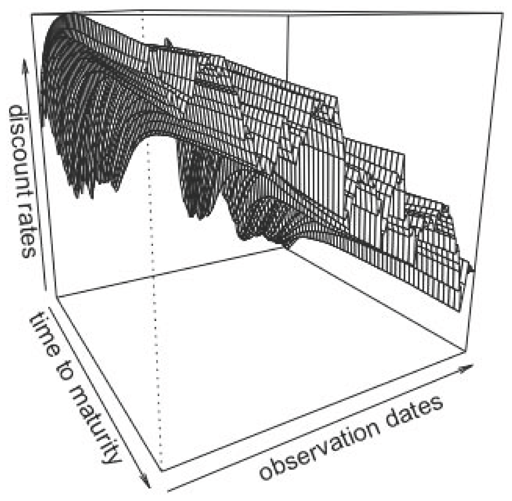
In Figure 2, we present the data that we use, and Table 1 contains a summary of these data; the minimum, maximum, median, first and third quartiles of the discount rates observed at given maturities. There are alternate cycles of increases and decreases of the discount rates, with a generally decreasing trend. Some of the discount rates, at the most recent dates, and lower maturities, are negative.
In the DNS framework, the spot interest rates observed at time t, for time to maturity are modeled as:
The factor loadings 1, and are used to represent the level, slope, and curvature of the Yield Curve. We obtain estimations of for each cross-section of yields by fixing , and doing a least squares regression on the factor loadings. The three time series associated to the loadings for each cross-section of yields, are those that we wish to forecast simultaneously, by using an RVFL model.
This type of model (DNS) cannot be used for no-arbitrage pricing as is, but it could be useful for example, for stressing the yield curve factors under the historical probability. It can however be made arbitrage-free, if necessary (see Diebold and Rudebusch 2013). We will benchmark the RVFL model applied to the three time series , against ARIMA (AutoRegressive Integrated Moving Average) and VAR (Vector AutoRegressive) models. Diebold and Li (2006) applied an autoregressive AR(1) model separately to each one of the parameters, .
We will apply to these parameters’ series: an ARIMA model (Hyndman and Khandakar 2008), and a Vector Autoregressive model (VAR, see Pfaff et al. 2008; Lütkepohl 2005); with the parameter of the DNS factor loadings, used as an hyperparameter for the time series cross-validation. In the RVFL and the VAR model, the number of lags is also used as an hyperparameter for the cross-validation. For the RVFL, the most recent values of are stored in matrix , as described in Section 2.3, ordered by date of arrival, whereas matrix contains the lags of the three series.
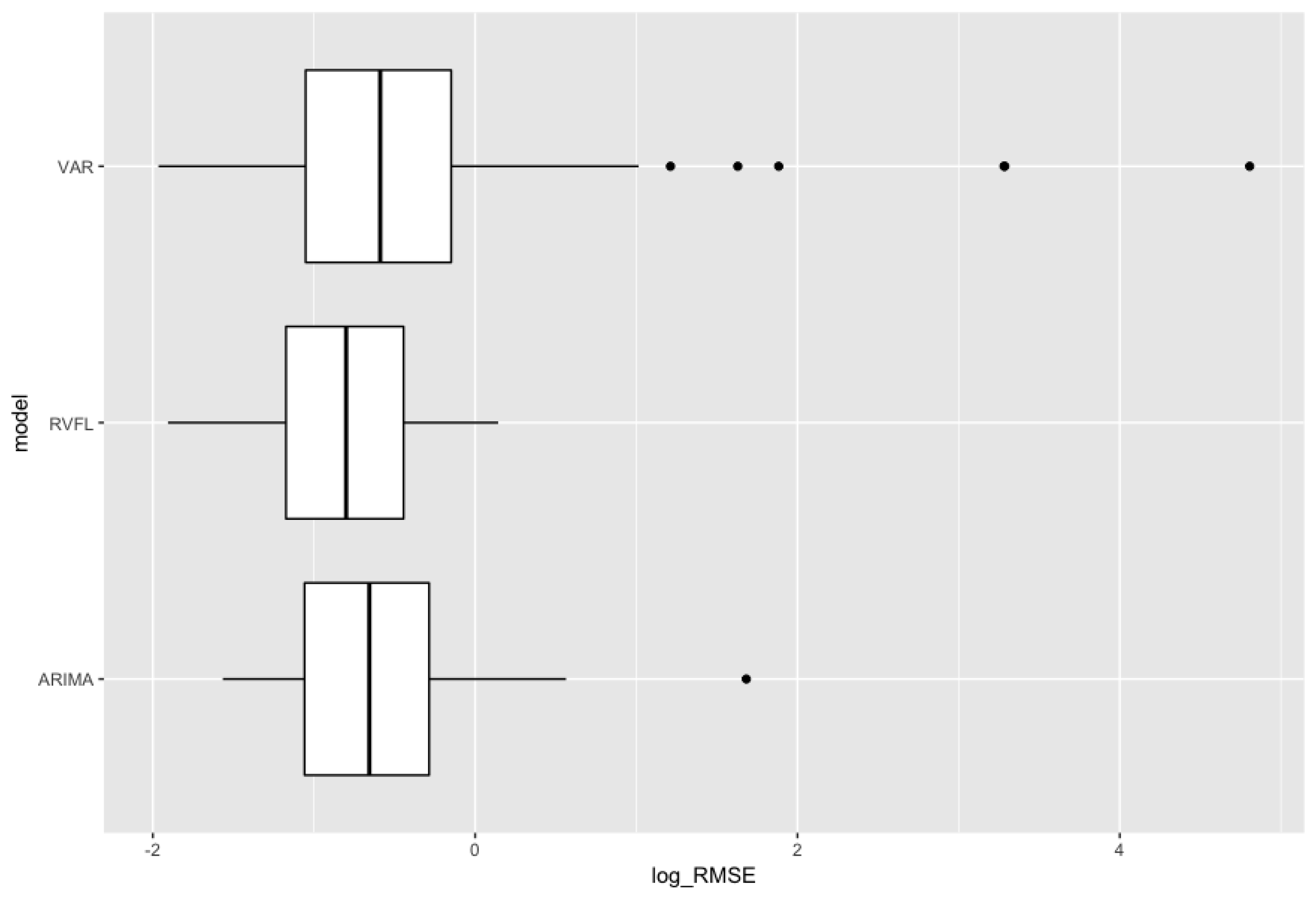
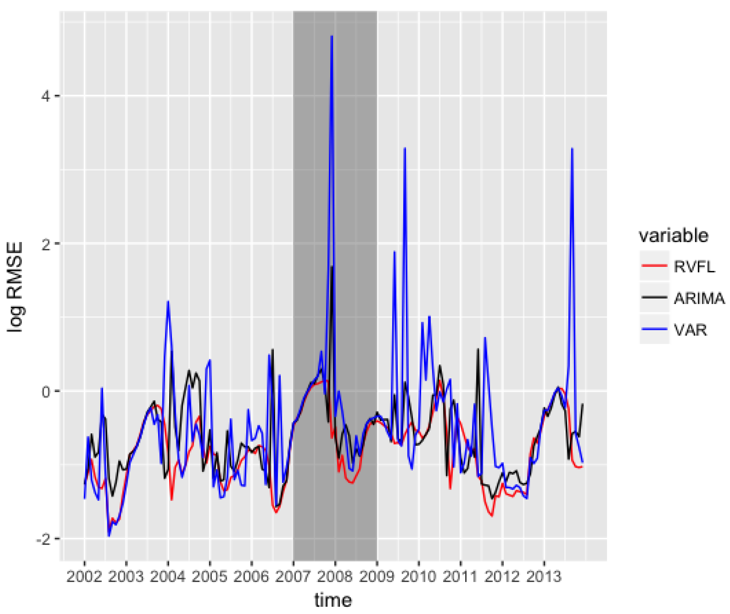
A rolling forecasting methodology (see Bergmeir et al. 2015) is implemented in order to obtain these benchmarks. A fixed 12 months-length window is established for training the model, and the following 12 months are used for testing; the origin of the training set is then advanced of 1 month, and the training/testing procedure is repeated. The measure of forecasting performance is the Root Mean Squared Error (). Figure 3 presents boxplots for the distribution of out-of-sample errors obtained in the cross-validation procedure, and Figure 4 presents the 12 months-ahead out-of-sample errors over time. ARIMA (separate (Hyndman and Khandakar 2008) ARIMA models applied to each series ) gives good results, as already suggested by Diebold and Li (2006). They are nearly comparable to results from RVFL, but a bit more volatile, with an outlier point observed on the box plot.
The unrestricted VAR model results include more volatility than the two other methods on this specific example, especially in the period of financial crisis between 2007 to 2009, as seen on Figure 4. Table 2 is to be read in conjuction with the box plot presented in Figure 3. It summarises the results obtained by the different methods on the out-of-sample . Table 3 contains confidence intervals around the mean of the differences between the three methods.
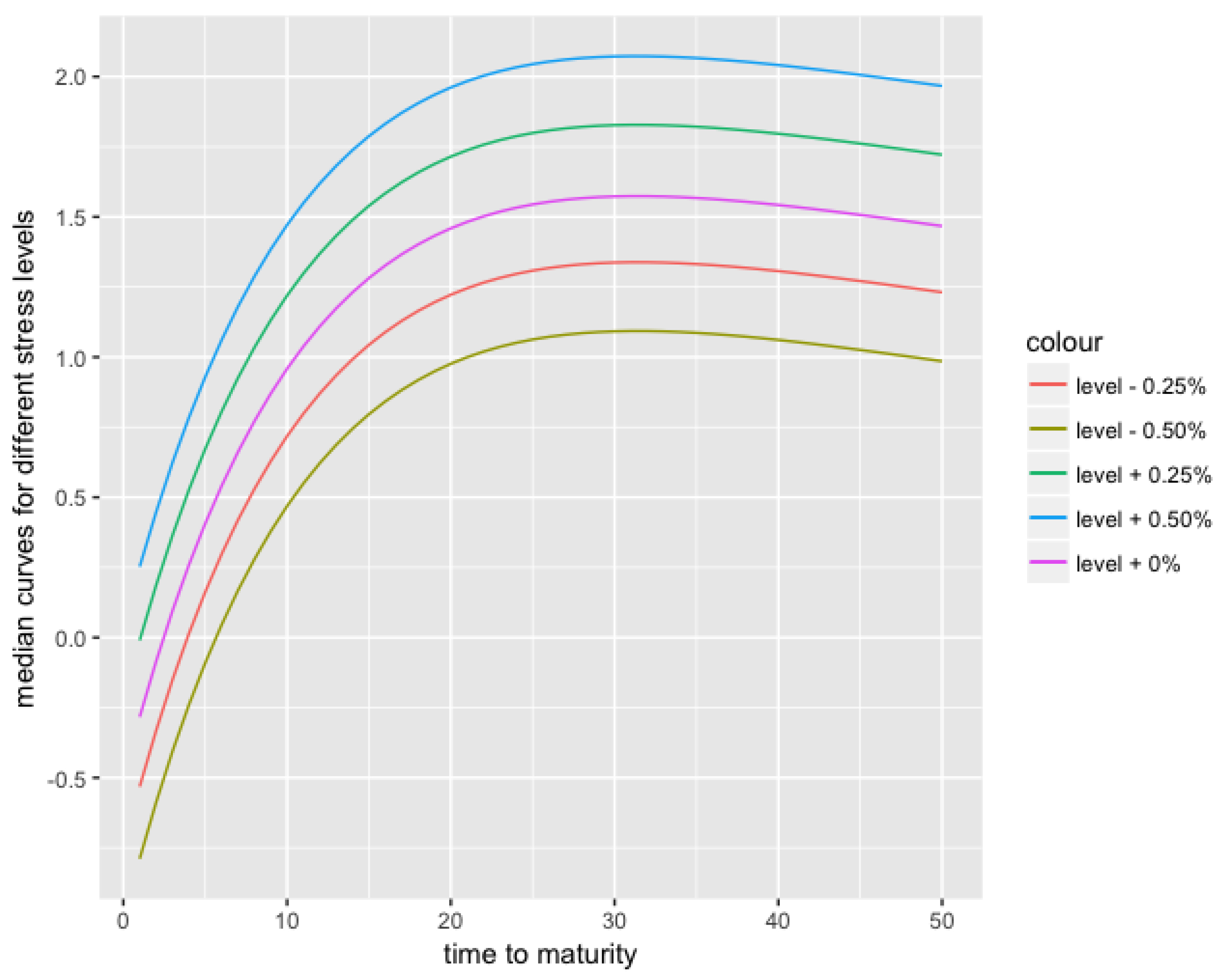
Another advantage of RVFL over ARIMA or AR(1) in this context is that it would be possible to add other variables to the RVFL regression, such as inflation, or dummy variables for external events, and combine their effects. It is also possible to stress one variable, and see the effects on the other variables, as presented in the Appendix A.1: the parameter is increased (from to ) and decreased (from to ), and the other parameters and forecasts move slightly, consecutively to these stresses. The corresponding median forecast curves for these stresses, and some additional ones, are presented in Figure 5.
3.2. Forecasting 1 Year, 10 Years and 20 Years Spot Rates
For this second example, we forecast the 1-year, 10-year and 20-year spot rates time series from the previous dataset, on a 12-month horizon. As described in the previous section, we use a rolling forecasting methodology, with a training window of 12 months’ length.
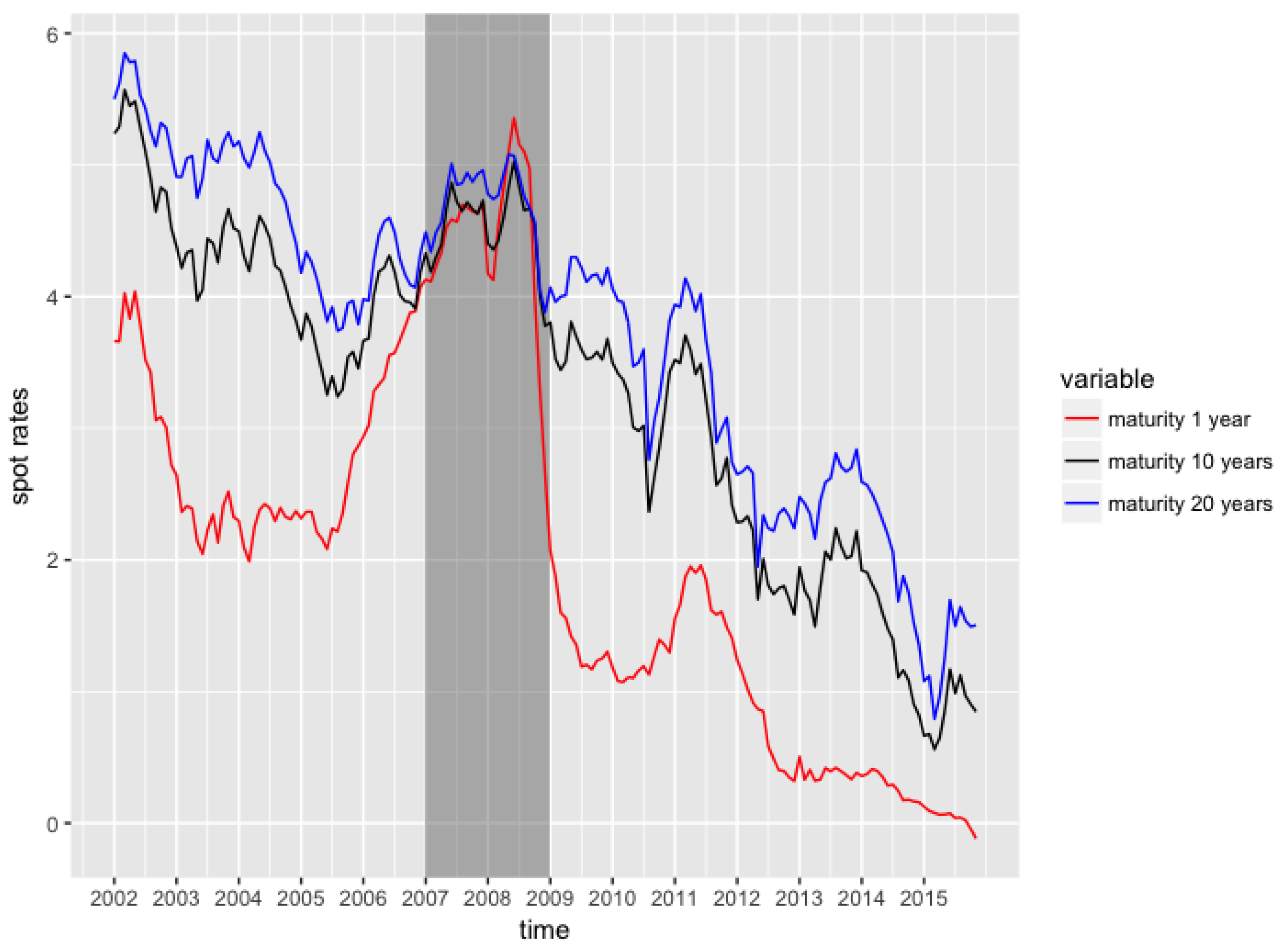
Figure 6 presents the three time series of data, and a summary of the data can be found in Table 4 and Table 5.
The three time series globally exhibit a decreasing trend, and are highly positively correlated. The spot rates for short-term maturities can also be negative, as it has been observed recently in 2016. The spreads between the spot rates time series are extremely narrow during the 2007–2009 crisis. The tables below (Table 6 and Table 7) contain the results of a comparison between the RVFL model and an unrestricted VAR model (with one lag, best parameter found) on the forecasting problem. The best RVFL model, with the lowest out-of-sample , uses one lag, four hidden nodes, and , .
3.3. Forecasting on a Longer Horizon, with a Longer Training Window
In this third example, as in Section 3.1, we apply the DNS framework to the forecasting of spot rates. However, in this example we have a longer training set (36 months), and a longer horizon for the test set (36 months as well). We use interest rate swaps data from the Federal Reserve Bank of St Louis website3, observed on a monthly basis from July 2000 to September 2016, with maturities equal to , and a tenor equal to three months.
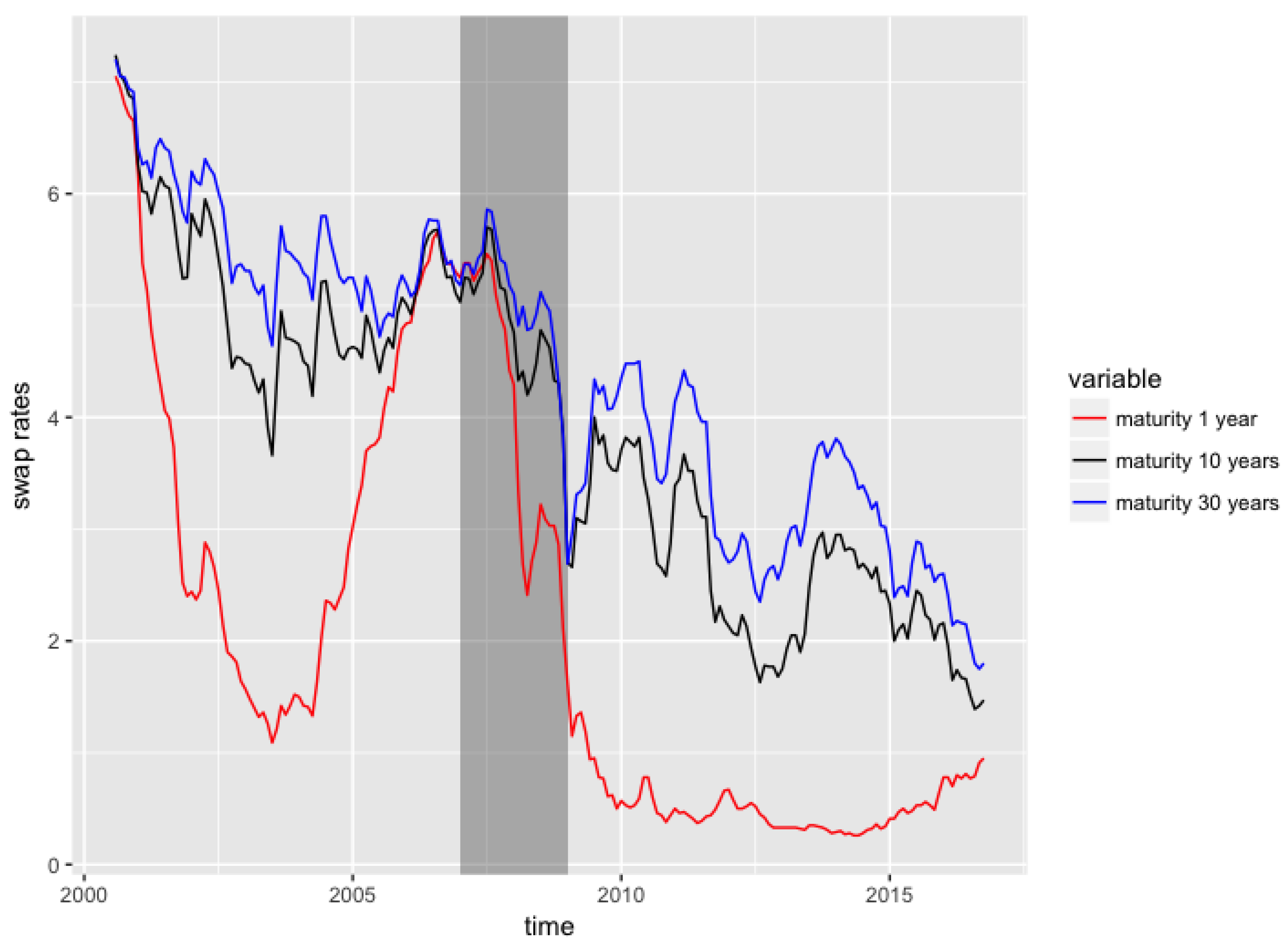
In Figure 7, we present three of the eight time series of swap rates, observed for time to maturities equal to and 30. The swap rates for different maturities generally exhibit a decreasing trend, and are nearly equal to 0 by the end of 2016, for the shortest maturities.
We also observe that the spreads between swap rates with different maturities start to narrow in 2006 until the end of 2007, and the swap rates for short term maturities are relatively high during the same period. This is the period corresponding to the Liquidity and Credit Crunch 2007–2008. Table 8 presents the descriptive statistics for these three time series.
All the swap rates (for all the maturities available) were then transformed into zero rates, by using a single curve calibration methodology (that is, ignoring the counterparty credit risk) with linear interpolation between the swaps’ maturities. Then, the Nelson & Siegel model was used for fitting and forecasting the curves in a DNS framework, with both auto.arima and the RVFL model presented in this paper, applied to the three factors. In the fashion of Section 3.1. However, now we obtain 36-month’s ahead forecasts, from a rolling training windows with a fixed 36 month’s length. The average out-of-sample are then calculated for each method.
The best hyperparameters—associated with the lowest out-of-sample average —for each model are obtained through a search on a grid of values. We have:
- DNS with ARIMA (auto.arima): (Nelson Siegel parameter).
- DNS with RVFL: number of lags for each series: 1, activation function: ReLU, number of nodes in the hidden layer: 45, , (RVFL parameters) and (Nelson Siegel parameter).
With these parameters, the results detailed in Table 9 are obtained, for the out-of-sample . A confidence interval around the difference of out-of-sample between ARIMA (applied to each one of the three factors) and RVFL is presented in Table 10.
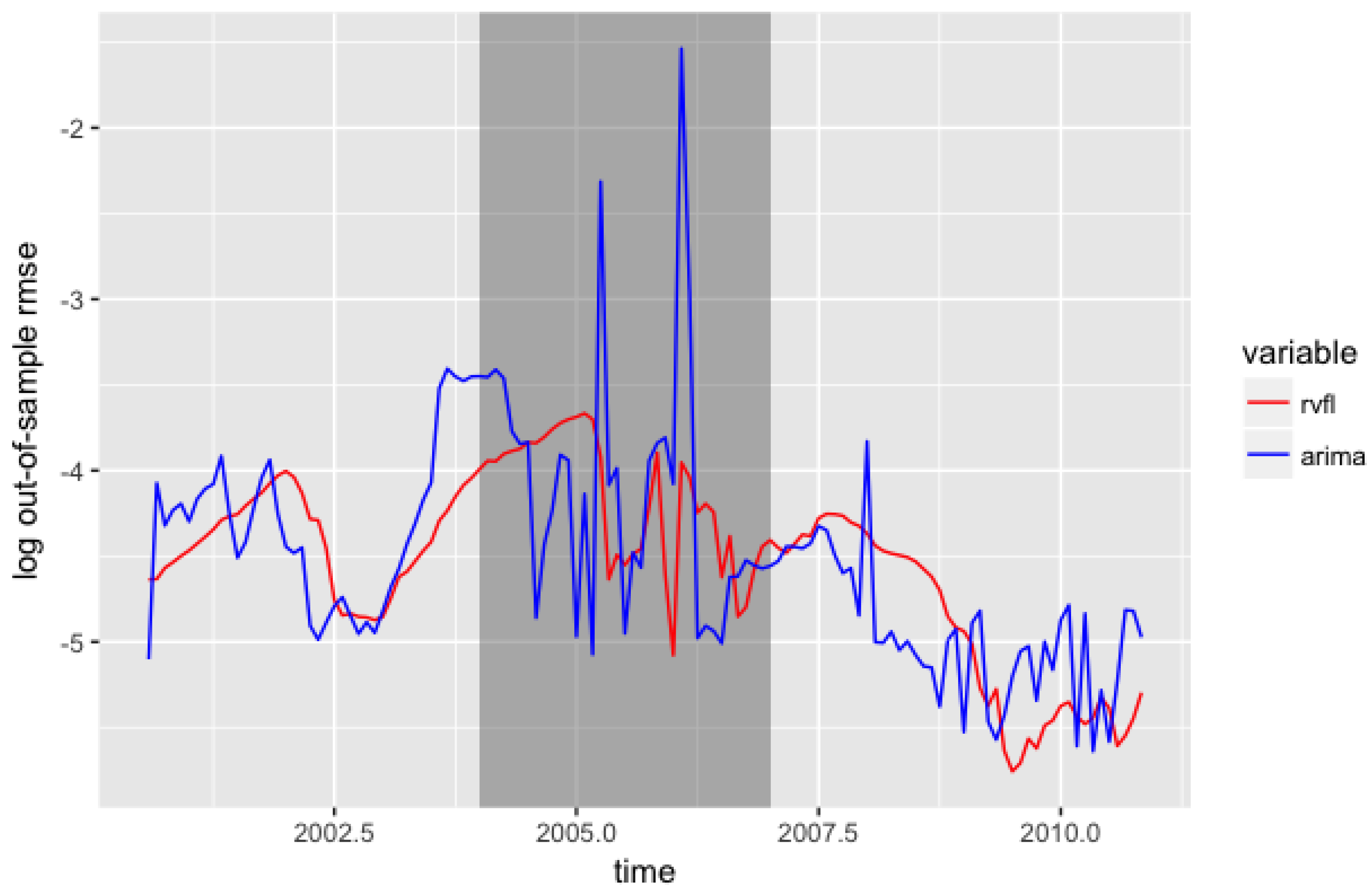
Figure 8 presents the evolution of the out-of-sample over the training/testing windows. The grey rectangle indicating the Liquidity and Credit crunch is larger here, because in this example, a training set starting in 2004 has its test set starting 36 months later, in 2007. Again, we observe that the results from the RVFL model exhibit a low out-of-sample error, along with a low volatility.
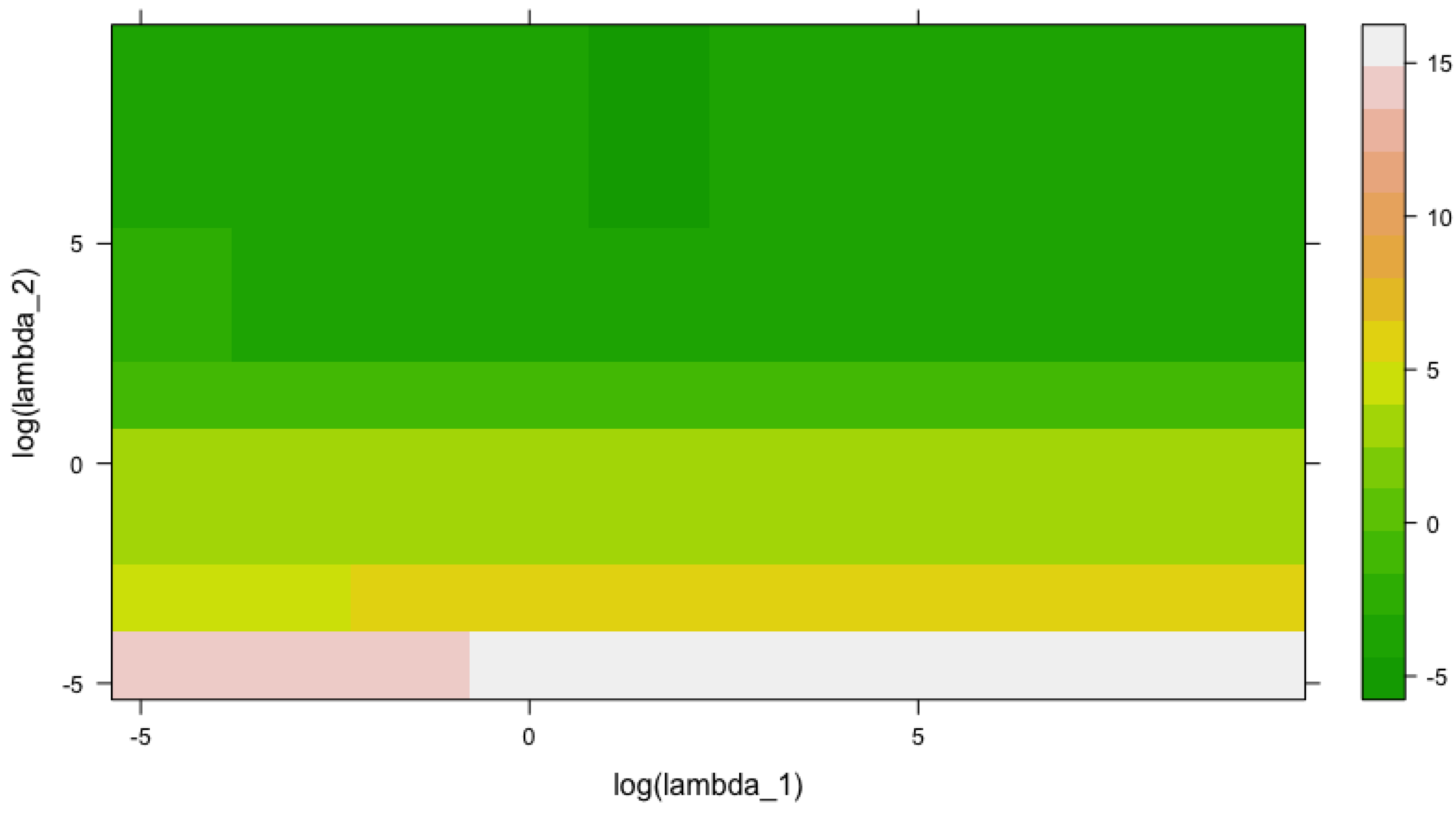
Figure 9, presents the convergence of the out-of-sample for the DNS + RVFL model from this section, as a function of and . and both range from to , with 10 equally-spaced points each (hence, a grid of 100 points .
The number of nodes in the hidden layer is equal to 45, and the value of , parameter from the Nelson and Siegel (1987) model presented in Section 3.1, is fixed and equal to 24. The one hundred points that we use for Figure 9 can be found in Appendix A.3.
There is a rectangular region at the top, in the middle of the figure, where the is the lowest. In this region, the lowest value of the out-of-sample is observed for and and the out-of-sample is equal to (75th point in Appendix A.3).
4. Conclusions
We present a model which could be used for multiple time series forecasting, based on a single layer quasi-randomized neural network. In this model, the lags of the different time series are used as in a dynamic regression model, and include the response variable lags. An additional layer of variables is added to the regression, whose nodes are not trained but obtained from a low discrepancy sequence. It is possible to add new variables to the regression, as indicators of special events, or to stress one variable, and observe the implied effect on the others’ forecast. The model is tested on raw historical spot rates, and in a Dynamic Nelson Siegel framework. It produces robust forecast results when compared to other usual (unpenalized) models in the same framework.
Author Contributions
Thierry Moudiki conceived and designed the experiments, with valuable inputs from Frédéric Planchet, Areski Cousin, and the reviewers. Thierry Moudiki performed the experiments. Thierry Moudiki analyzed the data. Thierry Moudiki wrote the paper.
Conflicts of Interest
The authors declare no conflict of interest.
Appendix A
Appendix A.1. Mean Forecast and Confidence Intervals for αi,t, i = 1,…,3 Forecasts
:
alpha1 y_lo80 y_hi80 y_lo95 y_hi95
13 0.7432724 0.6852024 0.8013425 0.6544620 0.8320829
14 0.7357374 0.6776673 0.7938074 0.6469269 0.8245478
15 0.7378042 0.6797342 0.7958742 0.6489938 0.8266147
16 0.7408417 0.6827717 0.7989118 0.6520313 0.8296522
17 0.7407904 0.6827204 0.7988604 0.6519800 0.8296009
18 0.7404501 0.6823801 0.7985201 0.6516396 0.8292605
19 0.7403603 0.6822903 0.7984303 0.6515498 0.8291707
20 0.7403981 0.6823281 0.7984681 0.6515876 0.8292085
21 0.7404788 0.6824087 0.7985488 0.6516683 0.8292892
22 0.7404786 0.6824086 0.7985487 0.6516682 0.8292891
23 0.7404791 0.6824091 0.7985491 0.6516686 0.8292895
24 0.7404758 0.6824058 0.7985458 0.6516654 0.8292863
:
alpha2 y_lo80 y_hi80 y_lo95 y_hi95
13 -1.250640 -1.351785 -1.149495 -1.405328 -1.095952
14 -1.243294 -1.344439 -1.142149 -1.397982 -1.088606
15 -1.241429 -1.342574 -1.140284 -1.396117 -1.086741
16 -1.243868 -1.345014 -1.142723 -1.398557 -1.089180
17 -1.244483 -1.345628 -1.143338 -1.399171 -1.089795
18 -1.241865 -1.343010 -1.140719 -1.396553 -1.087177
19 -1.240814 -1.341959 -1.139669 -1.395502 -1.086126
20 -1.240371 -1.341516 -1.139226 -1.395059 -1.085683
21 -1.240237 -1.341382 -1.139092 -1.394925 -1.085549
22 -1.240276 -1.341421 -1.139131 -1.394964 -1.085588
23 -1.240329 -1.341474 -1.139184 -1.395017 -1.085641
24 -1.240308 -1.341453 -1.139163 -1.394996 -1.085620
:
alpha3 y_lo80 y_hi80 y_lo95 y_hi95
13 4.584836 4.328843 4.757406 4.215410 4.870840
14 4.546167 4.307253 4.849862 4.163634 4.993482
15 4.527651 4.201991 4.803004 4.042913 4.962082
16 4.513810 4.216525 4.850160 4.048812 5.017874
17 4.517643 4.176214 4.828735 4.003502 5.001446
18 4.523109 4.203064 4.866713 4.027406 5.042371
19 4.522772 4.178489 4.848760 4.001079 5.026170
20 4.521846 4.191833 4.866066 4.013374 5.044524
21 4.521382 4.177560 4.854171 3.998472 5.033259
22 4.521451 4.186714 4.864755 4.007248 5.044222
23 4.521772 4.178995 4.857897 3.999300 5.037591
24 4.521862 4.184734 4.864155 4.004903 5.043987
Appendix A.2. Stressed Forecast (α1,t + 0.5%) and Confidence Intervals for αi,t, i = 1,…,3 Forecasts
:
alpha1 y_lo80 y_hi80 y_lo95 y_hi95
13 1.25 1.19193 1.30807 1.16119 1.33881
14 1.25 1.19193 1.30807 1.16119 1.33881
15 1.25 1.19193 1.30807 1.16119 1.33881
16 1.25 1.19193 1.30807 1.16119 1.33881
17 1.25 1.19193 1.30807 1.16119 1.33881
18 1.25 1.19193 1.30807 1.16119 1.33881
19 1.25 1.19193 1.30807 1.16119 1.33881
20 1.25 1.19193 1.30807 1.16119 1.33881
21 1.25 1.19193 1.30807 1.16119 1.33881
22 1.25 1.19193 1.30807 1.16119 1.33881
23 1.25 1.19193 1.30807 1.16119 1.33881
24 1.25 1.19193 1.30807 1.16119 1.33881
:
alpha2 y_lo80 y_hi80 y_lo95 y_hi95
13 -1.222568 -1.323713 -1.121423 -1.377256 -1.067880
14 -1.219401 -1.320546 -1.118256 -1.374089 -1.064713
15 -1.211361 -1.312506 -1.110216 -1.366049 -1.056673
16 -1.216213 -1.317358 -1.115068 -1.370901 -1.061525
17 -1.215266 -1.316411 -1.114121 -1.369954 -1.060578
18 -1.211474 -1.312619 -1.110329 -1.366162 -1.056786
19 -1.210329 -1.311474 -1.109183 -1.365017 -1.055640
20 -1.209610 -1.310755 -1.108465 -1.364298 -1.054922
21 -1.209648 -1.310793 -1.108503 -1.364336 -1.054960
22 -1.209601 -1.310746 -1.108456 -1.364289 -1.054913
23 -1.209688 -1.310833 -1.108542 -1.364376 -1.055000
24 -1.209653 -1.310798 -1.108508 -1.364341 -1.054965
:
alpha3 y_lo80 y_hi80 y_lo95 y_hi95
13 4.500390 4.244398 4.672961 4.130964 4.786394
14 4.482948 4.244035 4.786643 4.100415 4.930263
15 4.441841 4.116182 4.717194 3.957103 4.876272
16 4.441744 4.144459 4.778094 3.976746 4.945808
17 4.439609 4.098181 4.750701 3.925469 4.923413
18 4.447151 4.127105 4.790755 3.951448 4.966412
19 4.446164 4.101881 4.772152 3.924471 4.949562
20 4.445421 4.115407 4.789641 3.936949 4.968099
21 4.445411 4.101589 4.778200 3.922501 4.957289
22 4.445491 4.110754 4.788795 3.931287 4.968262
23 4.445937 4.103160 4.782062 3.923465 4.961756
24 4.446012 4.108885 4.788306 3.929053 4.968137
Appendix A.3. Out-of-Sample log(RMSE) as a Function of log(λ1) and log(λ2)
log_lambda1 log_lambda2 log_error
1 -4.605170 -4.605170 13.5039336
2 -3.070113 -4.605170 14.3538621
3 -1.535057 -4.605170 14.7912525
4 0.000000 -4.605170 14.8749375
5 1.535057 -4.605170 14.8928025
6 3.070113 -4.605170 14.8962203
7 4.605170 -4.605170 14.8975776
8 6.140227 -4.605170 14.8976494
9 7.675284 -4.605170 14.8976630
10 9.210340 -4.605170 14.8976715
11 -4.605170 -3.070113 3.9701229
12 -3.070113 -3.070113 4.9644144
13 -1.535057 -3.070113 5.2607788
14 0.000000 -3.070113 5.3208833
15 1.535057 -3.070113 5.3326856
16 3.070113 -3.070113 5.3351784
17 4.605170 -3.070113 5.3357136
18 6.140227 -3.070113 5.3358306
19 7.675284 -3.070113 5.3358557
20 9.210340 -3.070113 5.3358610
21 -4.605170 -1.535057 3.6692928
22 -3.070113 -1.535057 3.5643607
23 -1.535057 -1.535057 3.5063072
24 0.000000 -1.535057 3.4942438
25 1.535057 -1.535057 3.4904354
26 3.070113 -1.535057 3.4881352
27 4.605170 -1.535057 3.4888202
28 6.140227 -1.535057 3.4880668
29 7.675284 -1.535057 3.4886911
30 9.210340 -1.535057 3.4886383
31 -4.605170 0.000000 3.6224691
32 -3.070113 0.000000 3.8313407
33 -1.535057 0.000000 3.8518759
34 0.000000 0.000000 3.8163287
35 1.535057 0.000000 3.7993471
36 3.070113 0.000000 3.7948073
37 4.605170 0.000000 3.7937787
38 6.140227 0.000000 3.7935546
39 7.675284 0.000000 3.7935063
40 9.210340 0.000000 3.7934958
41 -4.605170 1.535057 -1.2115597
42 -3.070113 1.535057 -1.0130537
43 -1.535057 1.535057 -0.5841784
44 0.000000 1.535057 -0.3802817
45 1.535057 1.535057 -0.3109827
46 3.070113 1.535057 -0.2931830
47 4.605170 1.535057 -0.2891586
48 6.140227 1.535057 -0.2882824
49 7.675284 1.535057 -0.2880932
50 9.210340 1.535057 -0.2880524
51 -4.605170 3.070113 -2.0397856
52 -3.070113 3.070113 -3.1729003
53 -1.535057 3.070113 -3.8655596
54 0.000000 3.070113 -3.9279840
55 1.535057 3.070113 -3.9508440
56 3.070113 3.070113 -4.0270316
57 4.605170 3.070113 -4.0831569
58 6.140227 3.070113 -4.0953167
59 7.675284 3.070113 -4.0979447
60 9.210340 3.070113 -4.0985113
61 -4.605170 4.605170 -2.6779260
62 -3.070113 4.605170 -3.4704808
63 -1.535057 4.605170 -4.0404935
64 0.000000 4.605170 -4.2441836
65 1.535057 4.605170 -4.3657802
66 3.070113 4.605170 -4.3923094
67 4.605170 4.605170 -4.3862826
68 6.140227 4.605170 -4.3830293
69 7.675284 4.605170 -4.3820703
70 9.210340 4.605170 -4.3818486
71 -4.605170 6.140227 -3.5007058
72 -3.070113 6.140227 -3.8389274
73 -1.535057 6.140227 -4.1969545
74 0.000000 6.140227 -4.3400025
75 1.535057 6.140227 -4.4179718
76 3.070113 6.140227 -4.3797034
77 4.605170 6.140227 -4.3073100
78 6.140227 6.140227 -4.2866647
79 7.675284 6.140227 -4.2820357
80 9.210340 6.140227 -4.2810151
81 -4.605170 7.675284 -3.7236774
82 -3.070113 7.675284 -4.0057353
83 -1.535057 7.675284 -4.2699684
84 0.000000 7.675284 -4.3569254
85 1.535057 7.675284 -4.4156364
86 3.070113 7.675284 -4.3842360
87 4.605170 7.675284 -4.2759516
88 6.140227 7.675284 -4.2425876
89 7.675284 7.675284 -4.2346514
90 9.210340 7.675284 -4.2328863
91 -4.605170 9.210340 -3.7706268
92 -3.070113 9.210340 -4.0406387
93 -1.535057 9.210340 -4.2776907
94 0.000000 9.210340 -4.3498230
95 1.535057 9.210340 -4.4095778
96 3.070113 9.210340 -4.3860089
97 4.605170 9.210340 -4.2647179
98 6.140227 9.210340 -4.2273624
99 7.675284 9.210340 -4.2183911
100 9.210340 9.210340 -4.2163638
References
- Bergmeir, Christoph, Rob J. Hyndman, and Bonsoo Koo. 2015. A Note on the Validity of Cross-Validation for Evaluating Time Series Prediction. Monash Econometrics and Business Statistics Working papers 10/15. Clayton: Department of Econometrics and Business Statistics, Monash University. [Google Scholar]
- Bonnin, François, Florent Combes, Frédéric Planchet, and Montassar Tammar. 2015. Un modèle de projection pour des contrats de retraite dans le cadre de l’orsa. Bulletin Français d’Actuariat 14: 107–29. [Google Scholar]
- Boyle, Phelim P., and Keng Seng Tan. 1997. Quasi-monte carlo methods. In International AFIR Colloquium Proceedings. Sydney: Institute of Actuaries of Australia, vol. 1, pp. 1–24. [Google Scholar]
- Caruana, Rich. 1998. Multitask learning. In Learning to Learn. Berlin: Springer, pp. 95–133. [Google Scholar]
- Chakraborty, Kanad, Kishan Mehrotra, Chilukuri K. Mohan, and Sanjay Ranka. 1992. Forecasting the behavior of multivariate time series using neural networks. Neural Networks 5: 961–70. [Google Scholar] [CrossRef]
- Cormen, Thomas H. 2009. Introduction to Algorithms. Cambridge: MIT Press. [Google Scholar]
- Dehuri, Satchidananda, and Sung-Bae Cho. 2010. A comprehensive survey on functional link neural networks and an adaptive pso–bp learning for cflnn. Neural Computing and Applications 19: 187–205. [Google Scholar] [CrossRef]
- Diebold, Francis X., and Canlin Li. 2006. Forecasting the term structure of government bond yields. Journal of Econometrics 130: 337–64. [Google Scholar] [CrossRef]
- Diebold, Francis X., and Glenn D. Rudebusch. 2013. Yield Curve Modeling and Forecasting: The Dynamic Nelson-Siegel Approach. Princeton: Princeton University Press. [Google Scholar]
- Dutang, Christophe, and Petr Savicky. 2015. Randtoolbox: Generating and Testing Random Numbers. R Package version 1.17. Auckland: R-project. [Google Scholar]
- Exterkate, Peter, Patrick J. Groenen, Christiaan Heij, and Dick van Dijk. 2016. Nonlinear forecasting with many predictors using kernel ridge regression. International Journal of Forecasting 32: 736–53. [Google Scholar] [CrossRef]
- Hochreiter, Sepp, and Jurgen Schmidhuber. 1997. Long short-term memory. Neural Computation 9: 1735–80. [Google Scholar] [CrossRef] [PubMed]
- Hoerl, Arthur E., and Robert W. Kennard. 1970. Ridge regression: Biased estimation for nonorthogonal problems. Technometrics 12: 55–67. [Google Scholar] [CrossRef]
- Hyndman, Rob J., and Yeasmin Khandakar. 2008. Automatic time series forecasting: The forecast package for R. Journal of Statistical Software, 27. [Google Scholar] [CrossRef]
- Joe, Stephen, and Frances Y. Kuo. 2008. Notes on Generating Sobol Sequences. Available online: http://web.maths.unsw.edu.au/~fkuo/sobol/joe-kuo-notes.pdf (accessed on 3 January 2018).
- Lütkepohl, Helmut. 2005. New Introduction to Multiple Time Series Analysis. Berlin: Springer Science & Business Media. [Google Scholar]
- Nelson, Charles R., and Andrew F. Siegel. 1987. Parsimonious modeling of yield curves. Journal of Business 60: 473–89. [Google Scholar] [CrossRef]
- Niederreiter, Harald. 1992. Random Number Generation and Quasi-Monte Carlo Methods. Philadelphia: SIAM. [Google Scholar]
- Pankratz, Alan. 2012. Forecasting with Dynamic Regression Models. Hoboken: John Wiley & Sons, vol. 935. [Google Scholar]
- Pao, Yoh-Han, Gwang-Hoon Park, and Dejan J. Sobajic. 1994. Learning and generalization characteristics of the random vector functional-link net. Neurocomputing 6: 163–80. [Google Scholar] [CrossRef]
- Penrose, Roger. 1955. A generalized inverse for matrices. In Mathematical Proceedings of the Cambridge Philosophical Society. Cambridge: Cambridge University Press, vol. 51, pp. 406–13. [Google Scholar]
- Pfaff, Bernhard. 2008. VAR, SVAR and SVEC models: Implementation within R package vars. Journal of Statistical Software 27: 1–32. [Google Scholar] [CrossRef]
- Ren, Ye, P. Suganthan, N. Srikanth, and Gehan Amaratunga. 2016. Random vector functional link network for short-term electricity load demand forecasting. Information Sciences 367: 1078–93. [Google Scholar] [CrossRef]
- Rumelhart, David E., Geoffrey E. Hinton, and Ronald J. Williams. 1988. Learning internal representations by error propagation. In Neurocomputing: Foundations of Research. Cambridge: MIT Press, pp. 673–95. [Google Scholar]
- Schmidt, W. F., M. A. Kraaijveld, and R. P. Duin. 1992. Feedforward neural networks with random weights. In Proceedings: 11th IAPR International Conference on Pattern Recognition, 1992. Vol. II. Conference B: Pattern Recognition Methodology and Systems, The Hague, Netherlands, August 30–September 3. Piscataway: IEEE, pp. 1–4. [Google Scholar]
- Wickham, Hadley. 2016. Ggplot2: Elegant Graphics for Data Analysis. Berlin: Springer. [Google Scholar]
- Zhang, Le, and P. Suganthan. 2016. A comprehensive evaluation of random vector functional link networks. Information Sciences 367: 1094–105. [Google Scholar] [CrossRef]
| 1 | |
| 2 | Diebold and Rudebusch (2013): “there are by now literally hundreds of DNS applications involving model fitting and forecasting”. |
| 3 | Available at https://fred.stlouisfed.org/categories/32299. |
Figure 1.
General procedure for multiple time series forecasting with RVFL.

Figure 2.
Observed discount rates from Deutsche Bundesbank website, from 2002 to the end 2015.

Figure 3.
Distribution of out-of-sample , for ARIMA, VAR, and RVFL.

Figure 4.
Out-of-sample , for ARIMA, VAR, and RVFL over time.

Figure 5.
12 months-ahead median curves, for stressed yield curve level .

Figure 6.
1-year, 10-years and 20-years spot rates time series data.

Figure 7.
Swap rates data (in %) from St Louis Federal Reserve Bank, at maturities .

Figure 8.
Out-of-sample , for ARIMA and RVFL over time.

Figure 9.
Out-of-sample , as a function of and .


Table 1.
Summary of observed discount rates from Deutsche Bundesbank website, from 2002 to the end 2015.
Table 1.
Summary of observed discount rates from Deutsche Bundesbank website, from 2002 to the end 2015.
| Maturity | Min | 1st Qrt | Median | 3rd Qrt | Max |
|---|---|---|---|---|---|
| 1 | −0.116 | 0.858 | 2.045 | 3.072 | 5.356 |
| 5 | 0.170 | 1.327 | 2.863 | 3.807 | 5.146 |
| 15 | 0.711 | 2.616 | 3.954 | 4.702 | 5.758 |
| 30 | 0.805 | 2.594 | 3.962 | 4.814 | 5.784 |
| 50 | 0.749 | 2.647 | 3.630 | 4.590 | 5.467 |
Table 2.
Comparison of 12 months ahead out-of-sample (log(Root Mean Squared Error)), for the ARIMA(AutoRegressive Integrated Moving Average), RVFL, and VAR (Vector AutoRegressive).
Table 2.
Comparison of 12 months ahead out-of-sample (log(Root Mean Squared Error)), for the ARIMA(AutoRegressive Integrated Moving Average), RVFL, and VAR (Vector AutoRegressive).
| Method | Min. | 1st Qrt | Median | Mean | 3rd Qrt | Max. |
|---|---|---|---|---|---|---|
| RVFL | 0.1487 | 0.3092 | 0.4491 | 0.5041 | 0.6414 | 1.1535 |
| ARIMA | 0.2089 | 0.3470 | 0.5187 | 0.6358 | 0.7516 | 5.3798 |
| VAR | 0.1402 | 0.3493 | 0.5549 | 1.9522 | 0.8619 | 122.2214 |
Table 3.
95% confidence interval around the difference of out-of-sample .
| Method | Lower Bound | Upper Bound | Mean |
|---|---|---|---|
| RVFL-ARIMA | −0.2116 | −0.0518 | −0.1317 |
| RVFL-VAR | −3.1888 | 0.2927 | −1.4480 |
| ARIMA-VAR | −2.9937 | 0.3610 | −1.3163 |
Table 4.
Summary of the data for 1-year, 10-years and 20-years spot rates time series (in %).
| Min. | 1st Qrt | Median | Mean | 3rd Qrt | Max. | |
|---|---|---|---|---|---|---|
| 1-year rate | −0.116 | 0.858 | 2.045 | 2.062 | 3.072 | 5.356 |
| 10-years rate | 0.560 | 2.221 | 3.581 | 3.322 | 4.354 | 5.570 |
| 20-years rate | 0.790 | 2.685 | 4.050 | 3.782 | 4.830 | 5.850 |
Table 5.
Summary of data for 1-year, 10-year and 20-year spot rates time series.
| Correlations | 1-Year Rate | 10-Years Rate | 20-Years Rate |
|---|---|---|---|
| 1-year rate | 1.0000 | 0.8729 | 0.8118 |
| 10-years rate | 0.8729 | 1.0000 | 0.9900 |
| 20-years rate | 0.8118 | 0.9900 | 1.0000 |
Table 6.
Comparison of 12 months ahead out-of-sample , for the RVFL, and VAR.
| Method | Min. | 1st Qrt | Median | Mean | 3rd Qrt | Max. |
|---|---|---|---|---|---|---|
| RVFL | 0.1675 | 0.2906 | 0.4704 | 0.5452 | 0.6469 | 1.8410 |
| VAR | 0.1382 | 0.4025 | 0.6469 | 1.0310 | 1.0750 | 13.020 |
Table 7.
95% confidence interval around the difference of out-of-sample .
| Method | Lower Bound | Upper Bound | Mean |
|---|---|---|---|
| RVFL-VAR | −0.2622 | −0.7087 | −0.4854 |
Table 8.
Descriptive statistics of St Louis Federal Reserve data for 1-year, 10-years and 30-years swap rates (in %).
Table 8.
Descriptive statistics of St Louis Federal Reserve data for 1-year, 10-years and 30-years swap rates (in %).
| Maturity | Min. | 1st Qrt | Median | Mean | 3rd Qrt | Max. |
|---|---|---|---|---|---|---|
| 1 | 0.260 | 0.500 | 1.340 | 2.108 | 3.360 | 7.050 |
| 10 | 1.390 | 2.610 | 4.190 | 3.881 | 5.020 | 7.240 |
| 30 | 1.750 | 3.270 | 4.650 | 4.404 | 5.375 | 7.200 |
Table 9.
Descriptive statistics for out-of-sample , with rolling training window = 36 months, and testing window = 36 months.
Table 9.
Descriptive statistics for out-of-sample , with rolling training window = 36 months, and testing window = 36 months.
| Method | Min. | 1st Qrt | Median | Mean | 3rd Qrt | Max. | Std. Dev |
|---|---|---|---|---|---|---|---|
| ARIMA | 0.0036 | 0.0070 | 0.0104 | 0.0149 | 0.0161 | 0.2150 | 0.0213 |
| RVFL | 0.0032 | 0.0078 | 0.0115 | 0.0120 | 0.0148 | 0.0256 | 0.0055 |
Table 10.
95% confidence interval around the difference of out-of-sample .
| Method | Lower Bound | Upper Bound | Mean |
|---|---|---|---|
| RVFL-ARIMA | −0.0064 | 0.0007 | −0.0028 |
© 2018 by the authors. Licensee MDPI, Basel, Switzerland. This article is an open access article distributed under the terms and conditions of the Creative Commons Attribution (CC BY) license (http://creativecommons.org/licenses/by/4.0/).
Share and Cite
MDPI and ACS Style
Moudiki, T.; Planchet, F.; Cousin, A. Multiple Time Series Forecasting Using Quasi-Randomized Functional Link Neural Networks. Risks 2018, 6, 22. https://doi.org/10.3390/risks6010022
AMA Style
Moudiki T, Planchet F, Cousin A. Multiple Time Series Forecasting Using Quasi-Randomized Functional Link Neural Networks. Risks. 2018; 6(1):22. https://doi.org/10.3390/risks6010022
Chicago/Turabian StyleMoudiki, Thierry, Frédéric Planchet, and Areski Cousin. 2018. "Multiple Time Series Forecasting Using Quasi-Randomized Functional Link Neural Networks" Risks 6, no. 1: 22. https://doi.org/10.3390/risks6010022
Note that from the first issue of 2016, this journal uses article numbers instead of page numbers. See further details here.