Integrating the OpenSky Network into GNSS-R Climate Monitoring Research †

 , , and
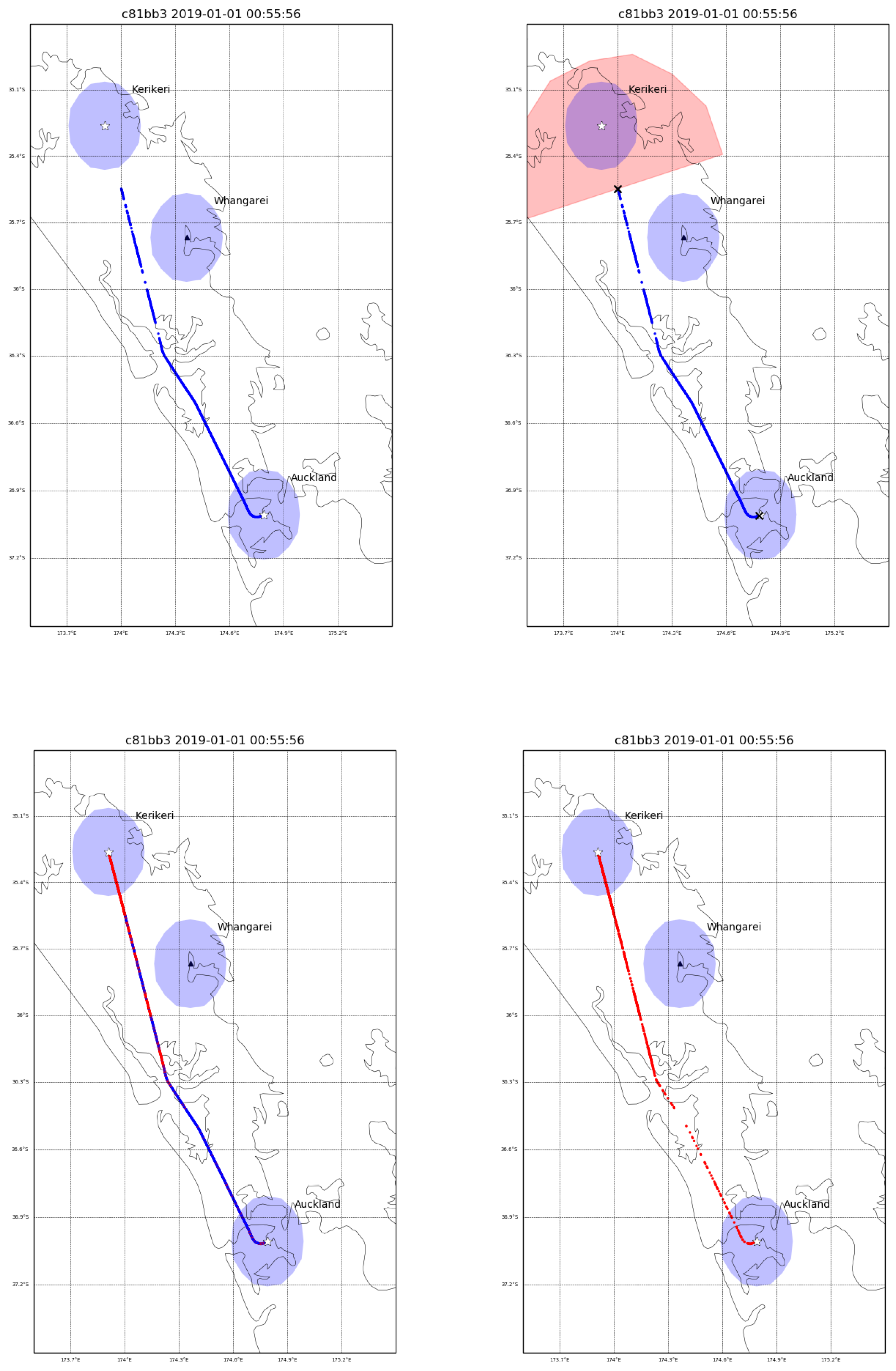
Abstract
:1. Introduction
1.1. Global Navigation Satellite System Reflectometry
1.2. NGRx: The Next Generation GNSS-R Receiver
2. Integrating the OpenSky Network Data into Our Research
2.1. Use Cases for the OpenSky Network Data
- minimum: to obtain a month’s-worth of state vectors for a single craft for comparison purposes;
- preferred: to also obtain API access to retrieve live tracking data for a single craft;
- ideal: to obtain a year’s-worth of state vectors for all 22 Q300 craft in Air New Zealand’s fleet and API access for live tracking of aircraft.
2.2. Data Retrieval and Processing
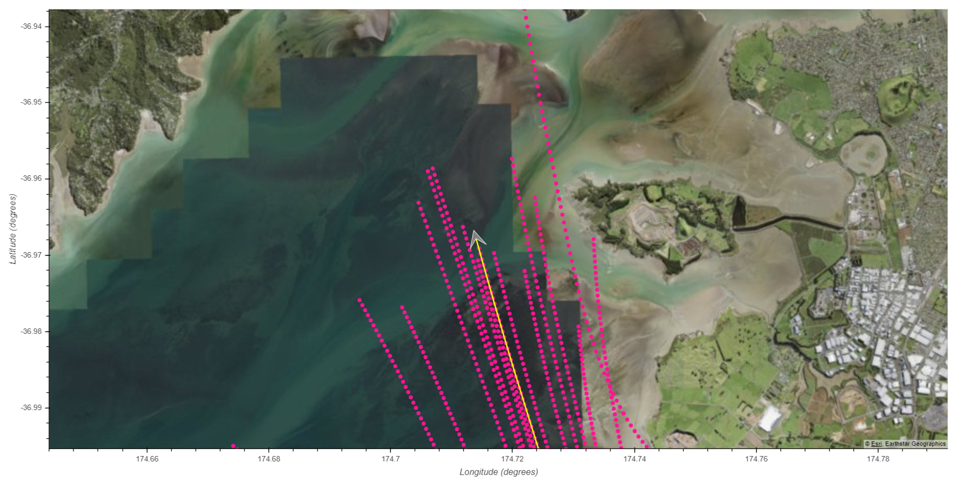
2.3. Estimating Flight Paths from the State-Vector Data
3. Visualising and Assessing the OpenSky Network Data
3.1. Visualising Historical GNSS-R Flight Data
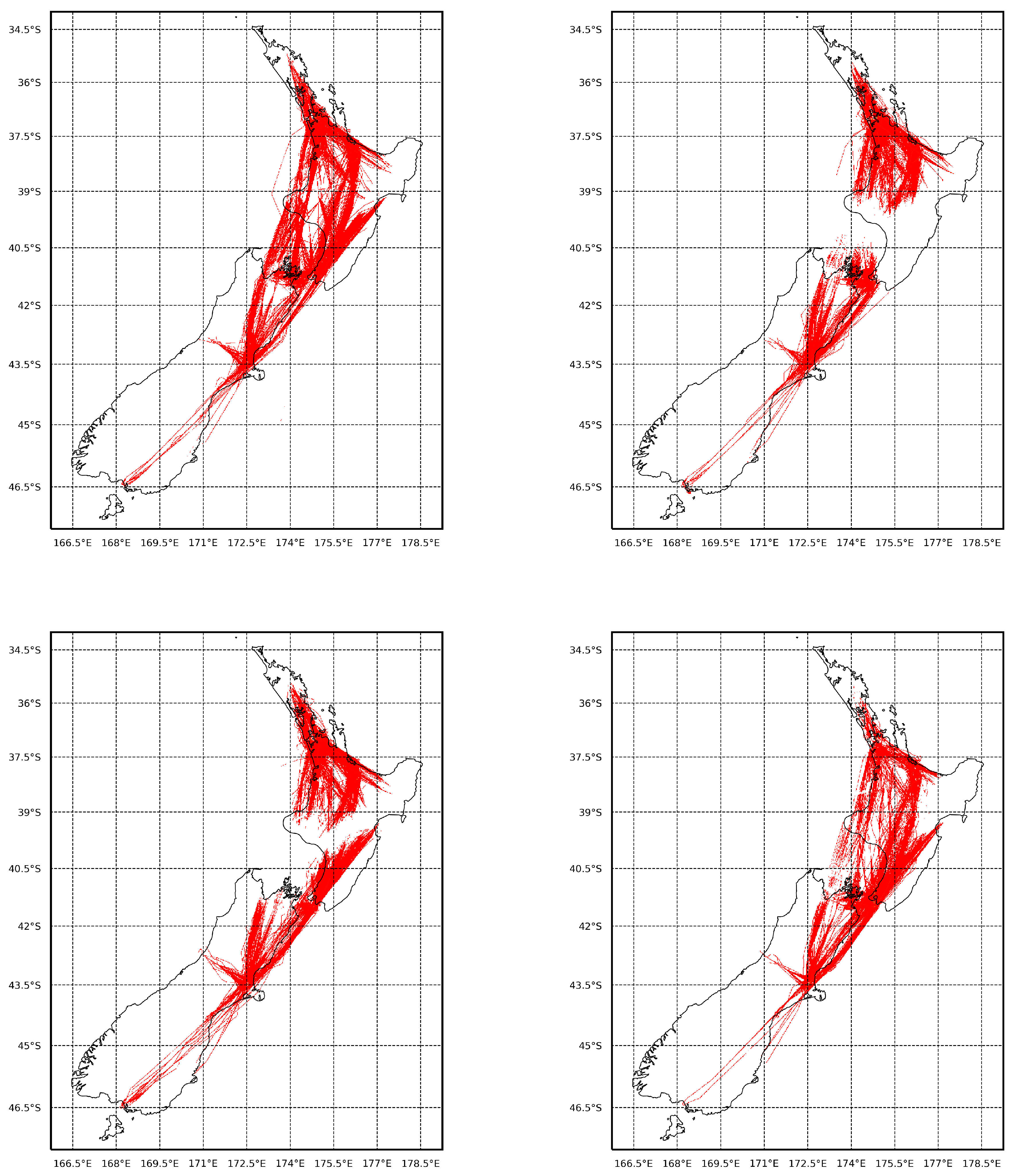
3.2. Visualising OpenSky Network ADS-B Coverage over New Zealand
4. Discussion and Future Plans
Author Contributions
Funding
Acknowledgments
Conflicts of Interest
References
- Garrison, J.; Katzberg, S.; Hill, M. Effect of sea roughness on bistatically scattered range coded signals from the global positioning system. Geophys. Res. Lett. 1998, 25, 2257–2260. [Google Scholar] [CrossRef]
- Ruf, C.S.; Atlas, R.; Chang, P.S.; Clarizia, M.P.; Garrison, J.L.; Gleason, S.; Katzberg, S.J.; Jelenak, Z.; Johnson, J.T.; Majumdar, S.J.; et al. New ocean winds satellite mission to probe hurricanes and tropical convection. Am. Meteor. Soc. 2016, 97, 385–395. [Google Scholar] [CrossRef]
- Ruf, C.S.; Chew, C.; Lang, T.; Morris, M.G.; Nave, K.; Ridley, A.; Balasubramaniam, R. A New Paradigm in Earth Environmental Monitoring with the CYGNSS Small Satellite Constellation. Sci. Rep. 2018, 8, 8782. [Google Scholar] [CrossRef] [PubMed]
- Jensen, K.; McDonald, K.; Podest, E.; Rodriguez-Alvarez, N.; Horna, V.; Steiner, N. Assessing L-Band GNSS-Reflectometry and Imaging Radar for Detecting Sub-Canopy Inundation Dynamics in a Tropical Wetlands Complex. Remote Sens. 2018, 10, 1431. [Google Scholar] [CrossRef]
- Chew, C.; Small, E. Soil Moisture Sensing Using Spaceborne GNSS Reflections: Comparison of CYGNSS Reflectivity to SMAP Soil Moisture. Geophys. Res. Lett. 2018, 45, 4049–4057. [Google Scholar] [CrossRef]
- Chew, C.; Reager, J.T.; Small, E. CYGNSS data map flood inundation during the 2017 Atlantic hurricane season. Sci. Rep. 2018, 8, 9336. [Google Scholar] [CrossRef] [PubMed]
- Schäfer, M.; Strohmeier, M.; Lenders, V.; Martinovic, I.; Wilhelm, M. Bringing up OpenSky: A large-scale ADS-B sensor network for research. In Proceedings of the ACM/IEEE International Conference on Information Processing in Sensor Networks, Berlin, Germany, 15–17 April 2014. [Google Scholar]
- McKinney, W. Data Structures for Statistical Computing in Python. In Proceedings of the 9th Python in Science Conference, Austin, TX, USA, 28 June–3 July 2010; pp. 56–61. [Google Scholar]


Publisher’s Note: MDPI stays neutral with regard to jurisdictional claims in published maps and institutional affiliations. |
© 2020 by the authors. Licensee MDPI, Basel, Switzerland. This article is an open access article distributed under the terms and conditions of the Creative Commons Attribution (CC BY) license (https://creativecommons.org/licenses/by/4.0/).
Share and Cite
Laverick, M.; Moller, D.; Ruf, C.; Musko, S.; O’Brien, A.; Linnabary, R.; Thomas, W.; Seal, C.; Wharton, Y. Integrating the OpenSky Network into GNSS-R Climate Monitoring Research. Proceedings 2020, 59, 11. https://doi.org/10.3390/proceedings2020059011
Laverick M, Moller D, Ruf C, Musko S, O’Brien A, Linnabary R, Thomas W, Seal C, Wharton Y. Integrating the OpenSky Network into GNSS-R Climate Monitoring Research. Proceedings. 2020; 59(1):11. https://doi.org/10.3390/proceedings2020059011
Chicago/Turabian StyleLaverick, Mike, Delwyn Moller, Christopher Ruf, Stephen Musko, Andrew O’Brien, Ryan Linnabary, Wayne Thomas, Chris Seal, and Yvette Wharton. 2020. "Integrating the OpenSky Network into GNSS-R Climate Monitoring Research" Proceedings 59, no. 1: 11. https://doi.org/10.3390/proceedings2020059011