Effects of Single-arc Blade Profile Length on the Performance of a Forward Multiblade Fan

1
National-Provincial Joint Engineering Laboratory for Fluid Transmission System Technology, Faculty of Mechanical Engineering and Automation, Zhejiang Sci-Tech University, Hangzhou 310018, China
2
Zhejiang Yilida Ventilator Co., Ltd., Taizhou 318056, China
*
Authors to whom correspondence should be addressed.
†
These authors contributed equally to this work.
Processes 2019, 7(9), 629; https://doi.org/10.3390/pr7090629
Submission received: 30 July 2019
/
Revised: 10 September 2019
/
Accepted: 12 September 2019
/
Published: 17 September 2019
(This article belongs to the Special Issue CFD Applications in Energy Engineering Research and Simulation)
Abstract
:The effects of single-arc blade profile length on the performance of a forward multiblade fan are investigated in this paper by computational fluid dynamics and experimental measurement. The present work emphasizes that the use of a properly reduced blade inlet angle (β1A) and properly improved blade outlet angle (β2A) is to increase the length blade profile, which suggests a good physical understanding of internal complex flow characteristics and the aerodynamic performance of the fan. Numerical results indicate that the gradient of the absolute velocity among the blades in model-L (reducing the blade inlet angle and improving blade outlet angle) is clearly lower than that of the baseline model and model-S (improving the blade inlet angle and reducing blade outlet angle), where a number of secondary flows arise on the exit surface of baseline model and model-S. However, no secondary flow occurs in model-L, and the flow loss at the exit surface of the volute (scroll-shaped flow patterns) for model-L is obviously lower than that of the baseline model at the design point. The comparison of the test results further shows that to improve the blade profile length is to increase the static pressure and the efficiency of the static pressure, since the improved static pressure of the model-L rises as much as 22.5 Pa and 26.2%, and the improved static pressure efficiency of the model-L rises as much as 5 % at the design flow rates. It is further indicated that increasing the blade working area provides significant physical insight into increasing the static pressure, total pressure, the efficiency of the static pressure and the total pressure efficiency.
1. Introduction
It is well known that centrifugal fans have been widely adopted to industrial application, such as cooling units in air-conditioning, heating, ventilating and air conditioning systems, and home appliance machines [1,2,3,4,5]. In general, it is essential for the centrifugal fan to improve its aerodynamic performance to achieve the purpose of energy conservation [5,6,7,8,9]. Many centrifugal fans with moderate efficiency and low aero-acoustic performances still need to be improved by making use of today’s technology. Velarde and Ballesteros [10] reported that to improve the blade number, tongue length and scroll contour is to improve the aerodynamic performance of a centrifugal blower. Younsi et al. [11] investigated that the internal flow of the blower for various rotational frequencies effects the performance characteristics of a turbo blower in a refuse collecting system. Lin and Huang [12] investigated that the performance of a centrifugal fan is affected by changing the blade inlet angle and the housing outlet geometry through experimental and computational methods.
Lun et al. [13] evaluated the total pressure and efficiency of a centrifugal fan by changing the impeller gap and blade inlet angle. Although varying the blade’s outlet angle does not appear to be very advantageous herein, it certainly shows the potential benefits of such a modification, especially in cases where the fan design is not optimal and demands vigorous enhancements [14]. The transient surface of the models with different outlet angles can be found [15,16,17]. Computational fluid dynamics (CFD) results were implemented to provide insight into revealing flow loss in the internal flow of fan. Thus, the prediction method of CFD is represented to study the internal flow mechanisms in the fan. The section of computational methodology includes solver descriptions of the Navier–Stokes and the used turbulence models associated, computational procedures for non-rotating and rotating components of the fan, gridding strategy and a study of grid density, and flow parameters for the performance of predicting the fan [18,19]. To validate the predictions of CFD for the performance of fan data, comparisons with one-fifth-scale model fan test data are provided [20]. The trend is quite straightforward: Increasing the outlet angle leads to a higher pressure rise and torque across the whole operating range, and vice versa.
Complex turbulent structures due to rotating Coriolis force and narrow blade passage in the internal flow of a forward multiblade fan play a dominant role in directly affecting the performance of the fan. Once these complex turbulent internal flows of the fan have been described, and the underlying internal flow mechanisms have been understood, new open questions will emerge in the internal flow of the fan. How do we restrain turbulent flow to reduce flow loss in the internal flow of our fan? In the low to mid-range flow rates, changing the outlet angle does not considerably affect the static efficiency of the fan, whereas the ensuing effects in the higher range are significant, and the impellers with larger outlet angles show a better performance.
Based on the above discussions, our study mainly focuses on the effects of the outlet angle of the impeller blades on the aerodynamic performance of the centrifugal fan for potential energy conservation. The origins and effects of a single-arc blade profile length on the performance of a forward multiblade fan are discussed with the emphasis on the understandings of the physical mechanisms of internal complex flow characteristics. Our work indicates that by reducing the blade inlet angle (β1A, β1A > 60°), improving the blade outlet angle (β2A, β2A < 175°) and increasing the blade’s working area may provide significant physical insight into increasing the static pressure and the efficiency of this static pressure. It gives insight into improving the aerodynamic load of fans to achieve the purpose of energy conservation. The performance of numerical results is quantitatively and qualitatively compared with that of the experimental results. This paper is organized as follows. In Section 2, governing equations and the numerical method will be briefly described at first. After that, the detailed numerical and experimental results are discussed. In final, some conclusions are addressed.
2. Governing Equations and Numerical Method
In the following section, the three-dimensional equation of fluid dynamics is implemented in fluid flow analysis of the computational domain [15,16]. The incompressible Reynolds Averaged Navier–Stokes (RANS) Turbulence Models are discretized by the finite volume method [16]. The equation of fluid dynamics is:
in which ρ is fluid density, and denote the components , and in the rectangular coordinate system in three directions, and are the average relative velocity components , and , denotes the reduced pressure, is the volume force component, and is the efficient viscosity coefficient [17,21]. The Re-Normalization Group (RNG) k-epsilon model is implemented in steady flow. The empirical formula of turbulence model RNG k-epsilon is as follows [22,23].
in which is the turbulent kinetic energy of laminar velocity gradient, denotes the turbulent kinetic energy, is the effect of compressible turbulent fluctuation expansion, , and are constants, and are the turbulent Prandtl numbers of the equation and ε equation, respectively. The above equations are solved by implementing the finite volume method. In first, the time discretization of the Navier–Stokes equations coupled with some governing equation for a pollutant is implemented in this paper. The spatial schemes are used to account for convective terms, viscous terms, mean pressure gradient effects and source terms associated with momentum or scalar equations, focusing on triangular meshes [20,24].
3. Computational Model and Grid of Fan
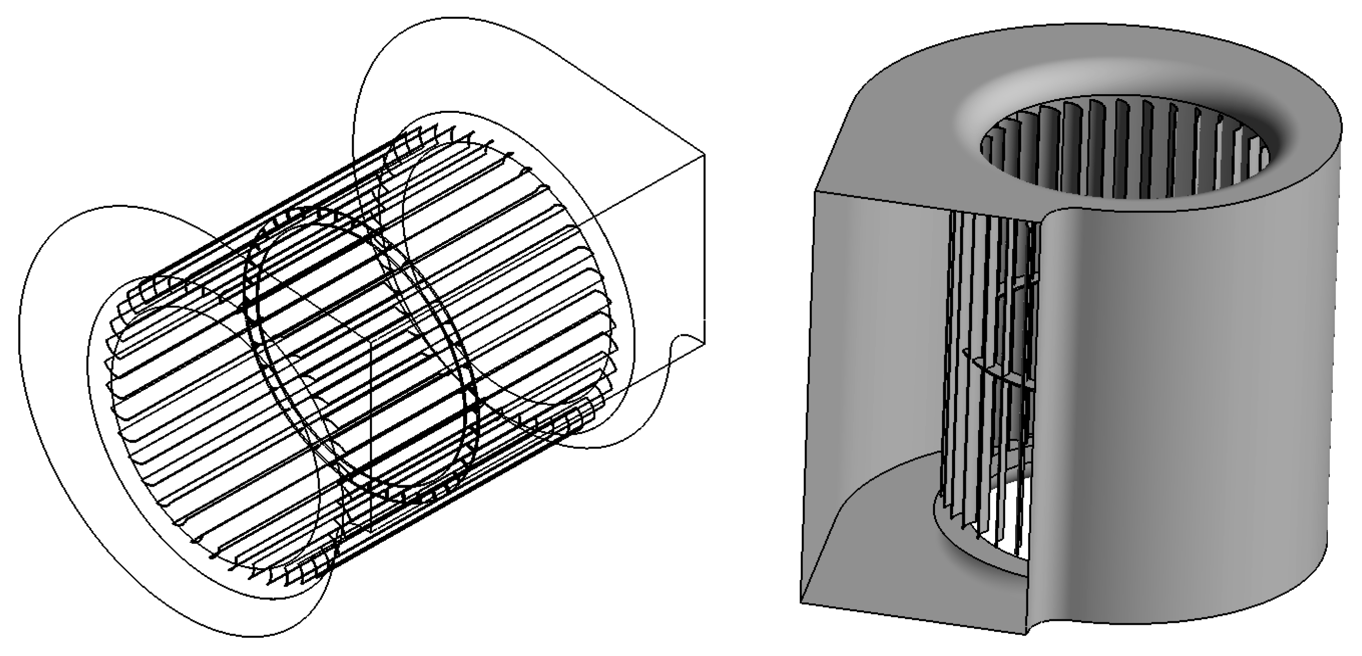
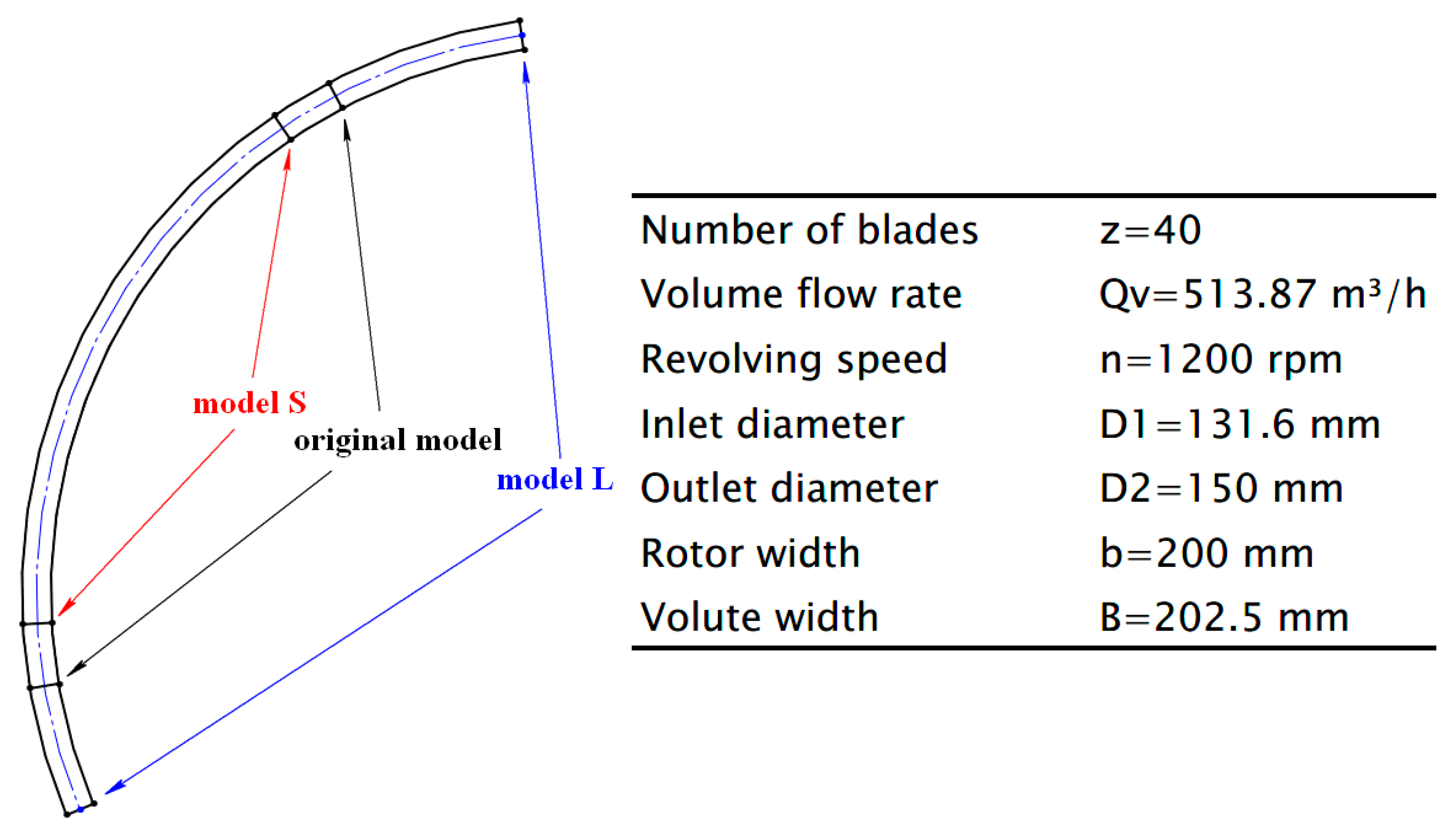
The forward multiblade centrifugal fan with a double-width double-inlet impeller is implemented in the current investigation. Figure 1 shows the double inlet radial fan with a forward curved blade. It consists of the impeller hub plate, volute, the mid-disc of impeller and the symmetry plane. The blade shape of test cases and some key parameters of the baseline model are presented in Figure 2. The complex vortex structure of the baseline model on the internal flow and performance is referred to in the previous work by Lun [13]. As shown in Figure 2, we can obtain that the blade profile of the baseline model is a single circular arc with the length of 10.904 mm; model-L refers to the model with a longer blade, and model-S with a shorter blade. Plotted in Figure 2, it is seen that the blade profile of model-L (reducing the blade inlet angle and improving blade outlet angle) is 150% that of the baseline model, and model-S (improving the blade inlet angle and reducing blade outlet angle) is 80%. The blade profiles of both modified models are still single circular arcs which are shown in Figure 2. The blade length of model-S, the baseline model and model-L increase successively in Figure 2.
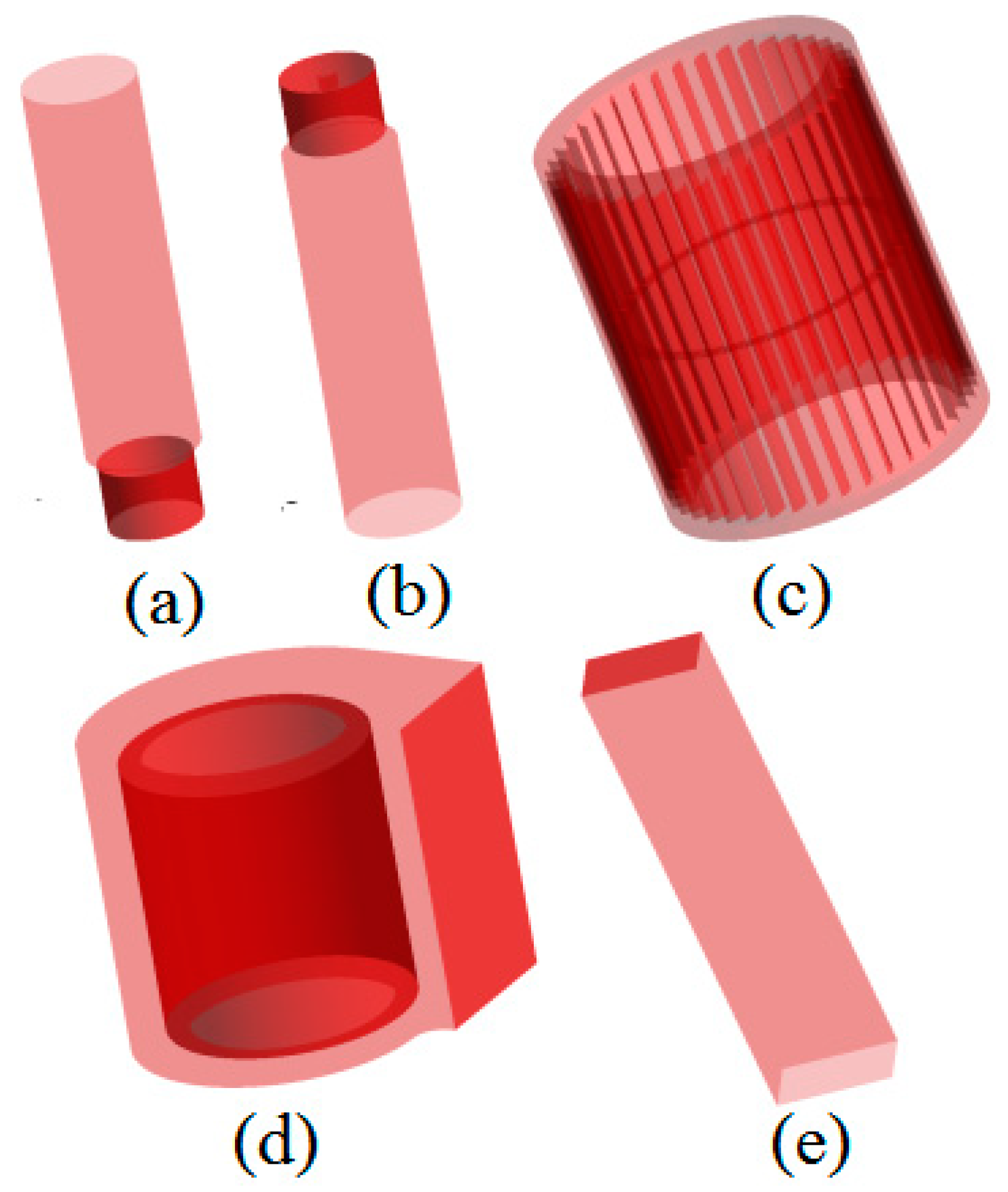
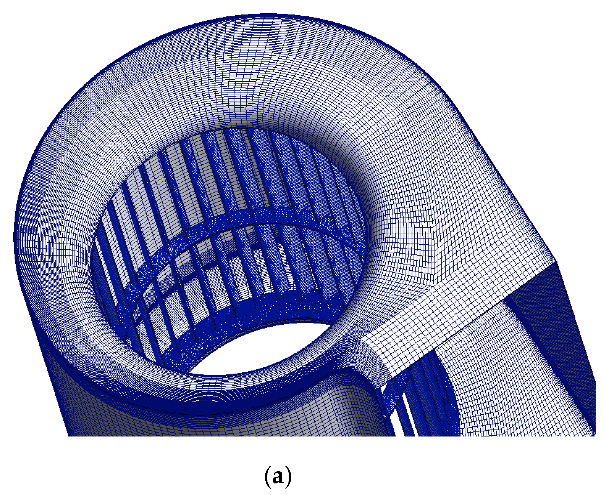
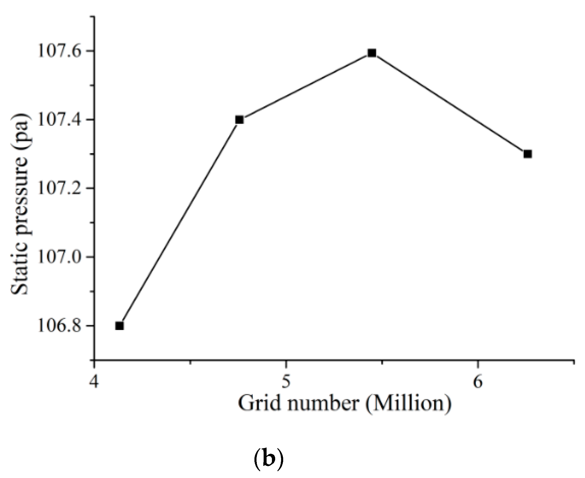
Table 1 shows the blade inlet angle and blade outlet angle of three models. As shown in Table 1, one can see that the blade inlet angles of the baseline model, model-S and model-L, are 84.83°, 91.27° and 71.34°, respectively, and the blade outlet angles of the baseline model, model-S and model-L are 152.36°, 146.69° and 170.13°, respectively. The numerical model of the radial fan is divided into five independent domains, as shown in Figure 3. Plotted in Figure 3, the impeller domain (domain 3) is set as the rotor and others are set as stators, while each domain is connected by an interface. The structured mesh is implemented for the whole fan model, and details of the numerical meshes of the volute and static pressure at a different number of grids are given in Figure 4. We can obtain that the change rate of static pressure is less than 1% at different mesh numbers. Thus, we can ignore the static pressure change. The numerical results are not affected by the number of grids. In all simulations, the ANSYS CFX software (CFX 16.0, Ansys, Canonsburg, PA 15317, USA) is implemented to study the internal complex flow of the forward multiblade centrifugal fan. The Multi Frames of Reference (MFR) technique is one such interface model. The MFR approach obtained by ANSYS CFX 16.0 is implemented to calculate the part of the impeller in the reference frame and the other parts in the stationary reference frame [12,13]. An interface is used at each junction where the frame change of reference takes place. There are two kinds of interface techniques available to exchange the information between the different frames of reference [12,13].
4. Results and Discussions
Finite element methods [24,25,26,27] and the finite volume method [28,29] are very effective tools to solve some partial differential equations (PDEs) on complex geometries, which is applied in a wide range of engineering and biomedical disciplines [30,31,32,33,34]. In this paper, the finite volume method is implemented to calculate the NS equation. Numerical simulations are carried out using steady RANS based on the RNG k-ε turbulence model in our studies. The empirical formula of the turbulence model RNG k-epsilon is introduced in detail in Section 2. The mass flow rate is implemented as the inlet condition, and static pressure is implemented as the outlet condition. The wall condition is no slip boundary. It is well known that a moving fluid in contact with a solid body will not have any velocity relative to the body at the contact surface. This condition of not slipping over a solid surface has to be satisfied by a moving fluid. The second order upwind discretized form is used for all cases in incompressible flows [21,22]. The second order upwind discretized form is mainly based upon a coupled solution of the nonlinear finite difference equations according to the multigrid technique. Calculations have been made of the driven turbulent flow for several Reynolds numbers and finite difference grids. In comparison with the hybrid discretized form, the second order upwind discretized form is somewhat more accurate, but it is not monotonically accurate with mesh refinement.
4.1. Numerical Verification
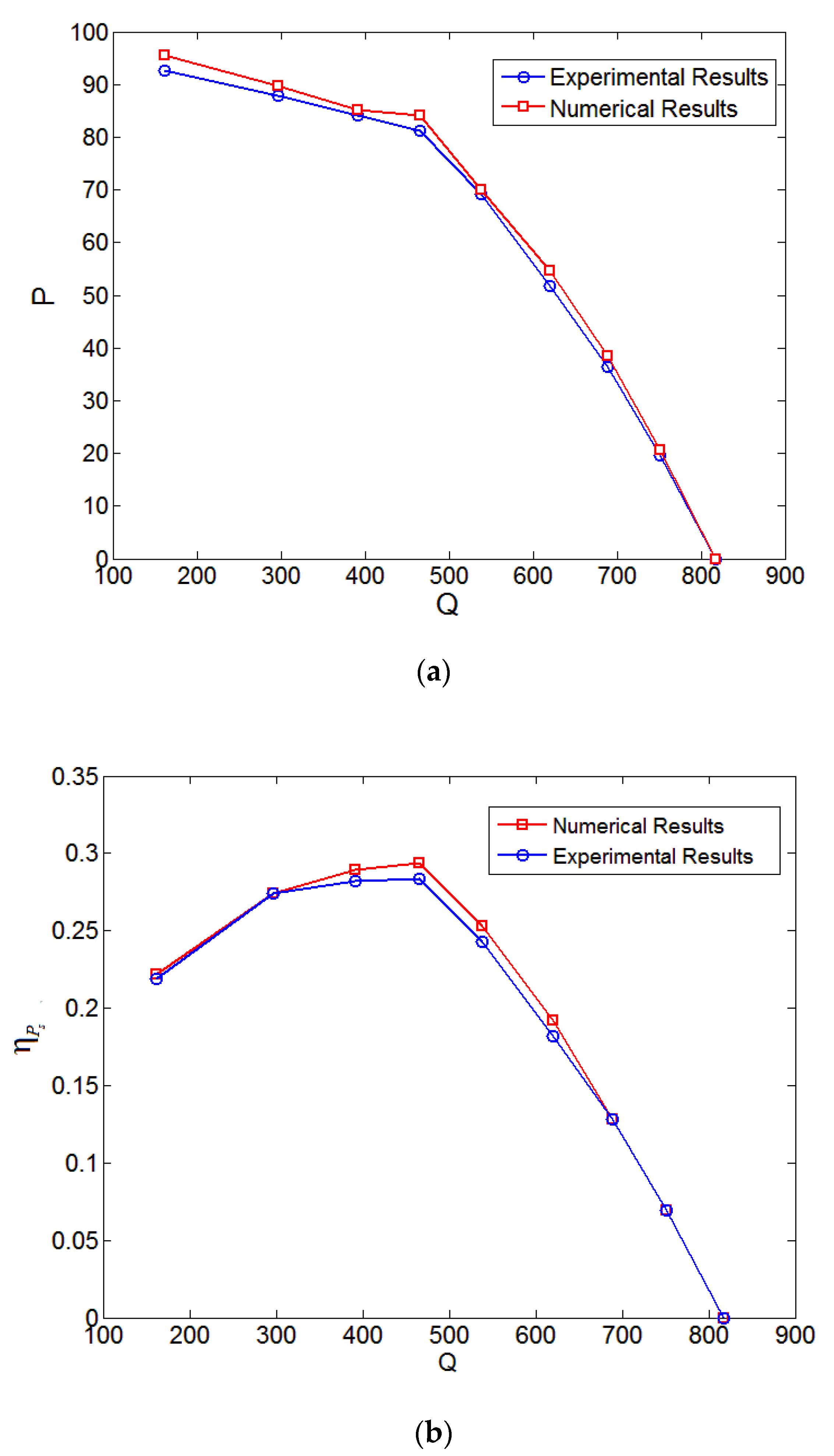
In order to confirm the accuracy of numerical results, the baseline model is implemented to study its static pressure and the efficiency of this static pressure at various flow rates. Figure 5 shows the comparison of static pressure as well as the static pressure efficiency between numerical results and experimental results. As shown in Figure 5, one can clearly see that the static pressure (P, Pa) decreases with the increase of flow rate (Q, m3/h) in both the experiment and numerical simulation. It is also obtained that the static pressure curve and the static pressure efficiency curve of the baseline model is well consistent with the experimental results at various flow rates, which demonstrates that the numerical accuracy is reliable.
4.2. Complex Internal Flow in Different Forward Multiblade Fans
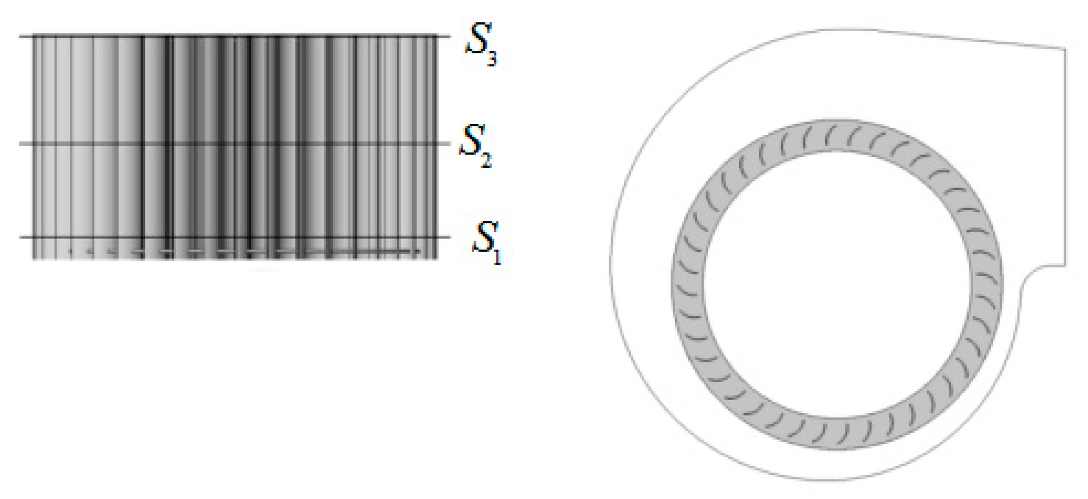
In the following section, complex internal flow in different forward multiblade fans will be introduced. The analysis refers to the centrifugal fan operating at three mass flow rate conditions of 0.0403 kg/s (0.235Qn), 0.1713 kg/s (Qn) and 0.2809 kg/s (1.640Qn). Figure 6 shows the overview of the flow behavior within the impeller with the absolute velocity contours. Plotted in Figure 6, S1, S2 and S3 represent the cutting planes at the hub, at the mid-span and at the tip of the impeller, respectively.
Figure 7 shows the absolute velocity at different heights within the impeller. As shown in Figure 7, it is obviously seen that the gradient of the absolute velocity among the blades decreases with the successive increase of the blade length of model-S, the baseline model and model-L at the cross section of S1, S2 and S3, which mainly indicates that the size of the flow separation among the blades becomes smaller with increasing the blade outlet angle. We can see that on the hub surface (S1), the velocity difference between inlet and outlet of the impeller increases, and the velocity gradient in the impeller passage of model-L is more uniform than that of others. The area of the low velocity region at the inlet of the impeller decreases because of lengthening the blade in model-L. The average velocity decreases with the increase of axial height in the impeller passage. The main reason is that the flow in the passage of the tip cutting plane (S3) is greatly affected by the inflow near the inlet of the volute.
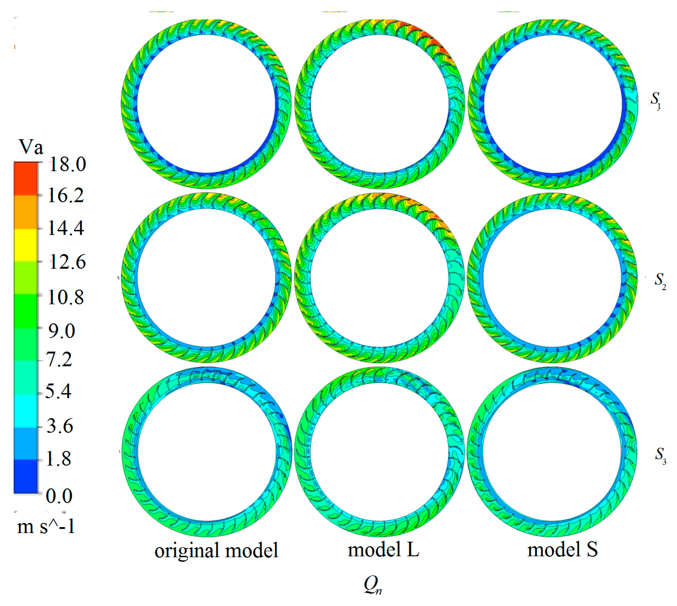
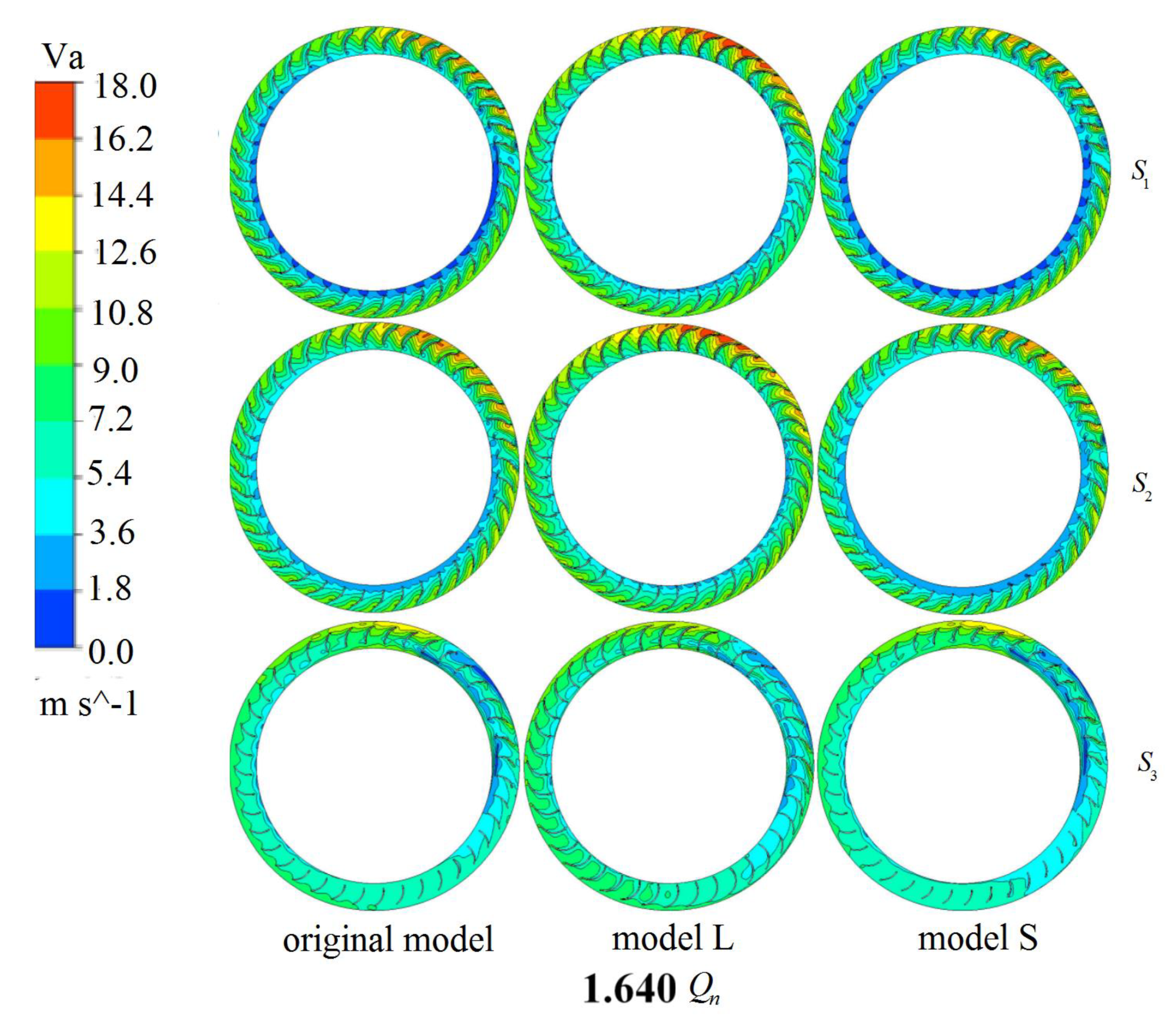
Figure 8 shows the absolute velocity at different heights within the impeller at design point Qn. It is clearly observed that at the design point, the high velocity region exists at the impeller outlet of model-L at the hub plane (S1) and midspan (S2). However, model-L possesses more uniform velocity distribution in the impeller passage than that of the baseline model and model-S. Figure 9 shows the absolute velocity at different heights within the impeller at 1.64Qn. One can see that the high absolute velocity region in model-L is obviously larger than that of the baseline model and model-S. A large number of low absolute velocity regions occur at the inlet of blades in the baseline model and model-S at sections of S1 and S2. Nevertheless, the gradient of the absolute velocity among the blades in model-L is clearly lower than that of the baseline model and model-S.
From Figure 7 to Figure 9, it is also obtained that the high velocity region at the impeller outlet moves toward the outlet of volute, and the difference of velocity in the blade passage increases accordingly with the increase of the mass flow rate. It is also noted that the high absolute velocity region in model-L is obviously higher than that of the baseline model and model-S. However, the gradient of the absolute velocity among the blades in model-L is clearly lower than that of the baseline model and model-S. It is further found that the gradient of the absolute velocity among the blades decreases in model-L, which brings about the decreasing size of the flow separation among the blades.
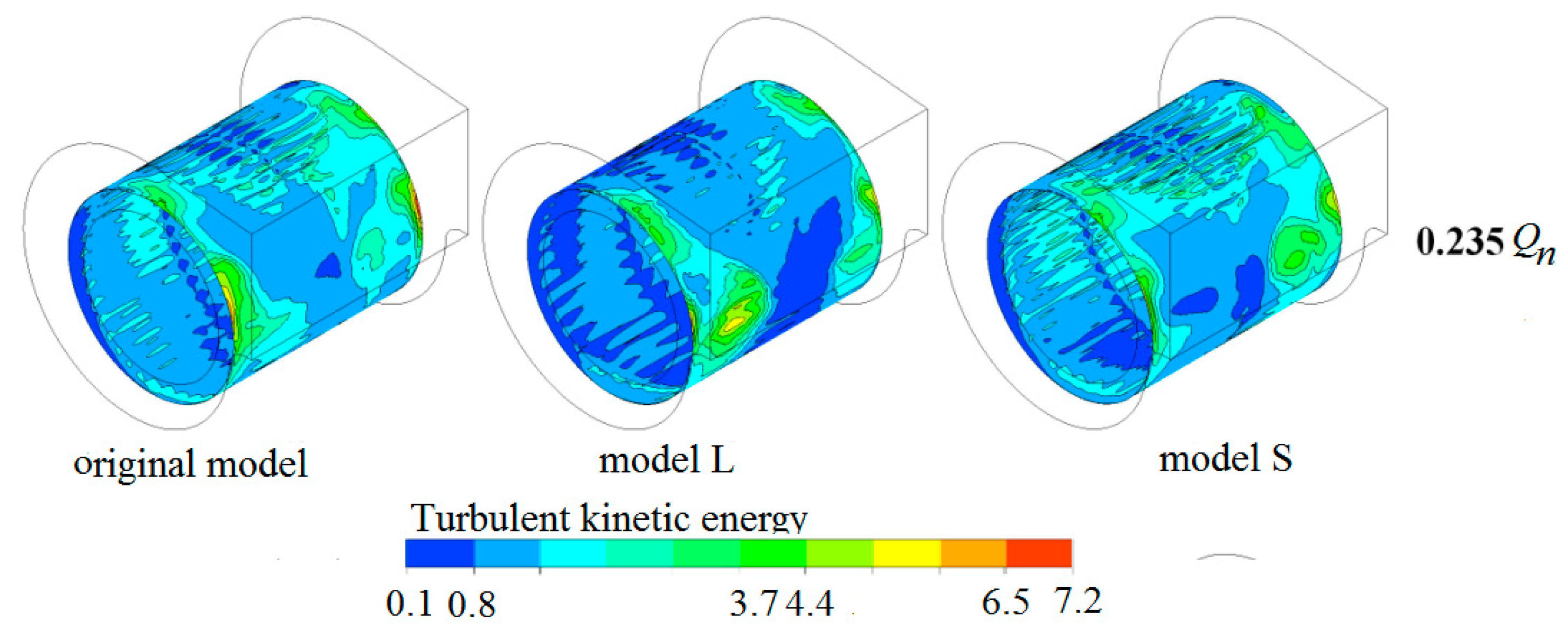
Figure 10 delineates the turbulence kinetic energy (TKE) of impeller outlet at 0.235Qn. It is clearly observed that the high turbulence kinetic energy area in the baseline model occurs at the inlet of the volute. Meanwhile, the high turbulence kinetic energy area in model-L and model-S also occurs at the inlet of the volute. It is noted that for the turbulence kinetic energy, no significant difference occurs near the inlet of the volute in the baseline model, model-L and model-S.
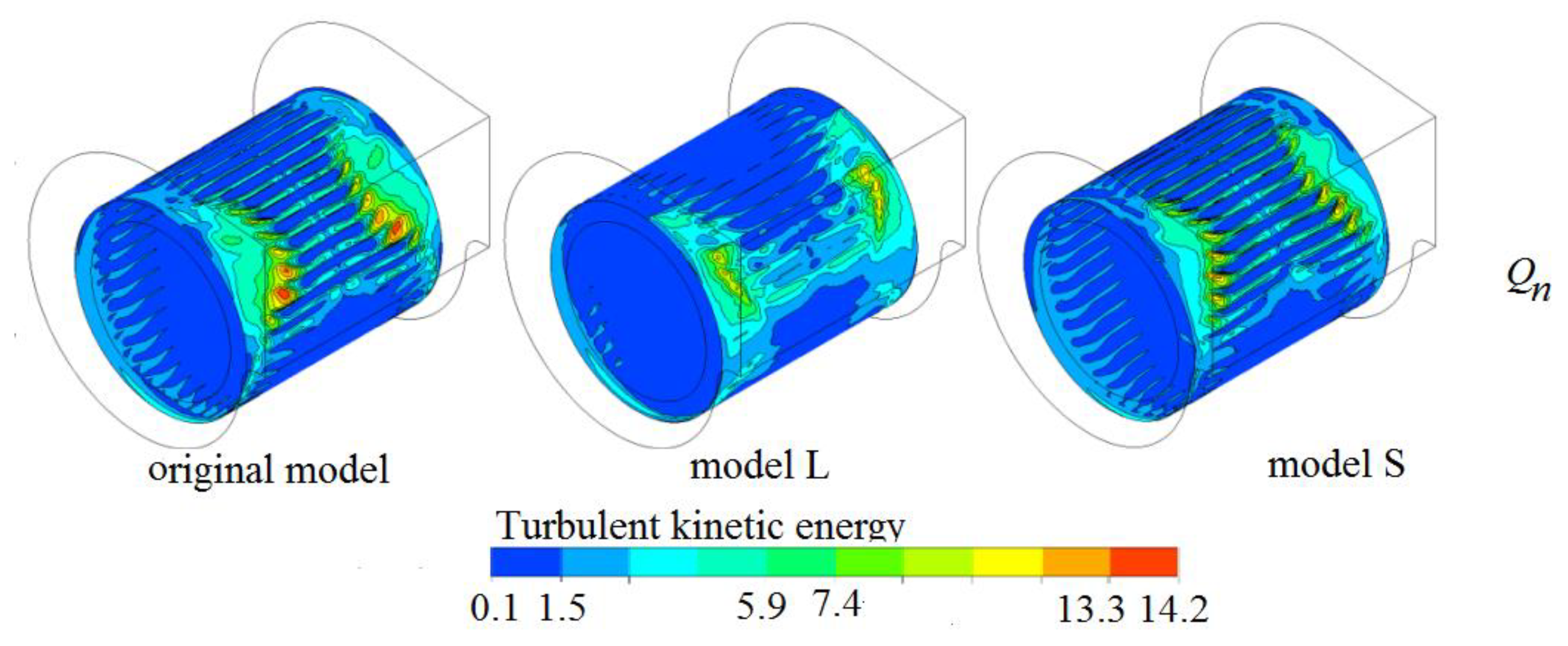
Figure 11 shows the TKE of the impeller outlet at the design point Qn. One can obviously see that at design point Qn, the turbulence kinetic energy area near the inlet of the volute for model-L is lower than that of baseline model and model-S. It is also noted that the TKE at the impeller outlet of model-L and model-S is obviously reduced as compared with that of the baseline model and model-S.
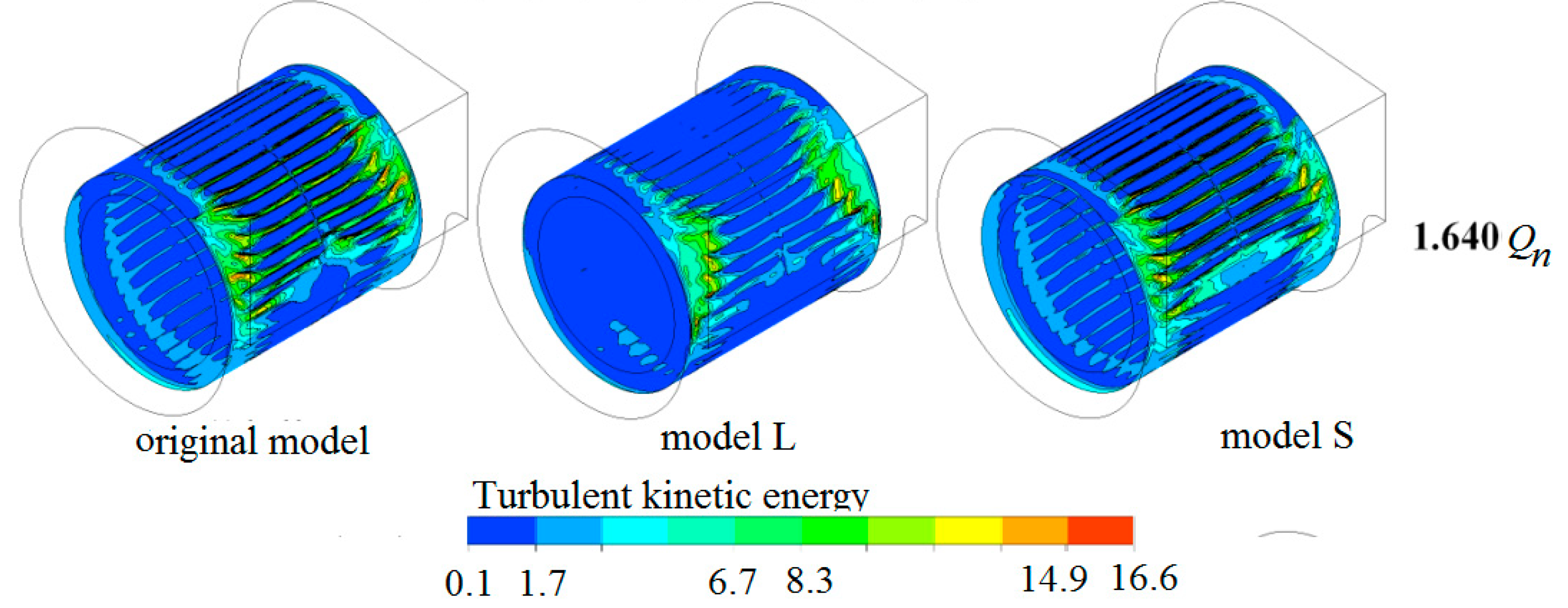
Figure 12 demonstrates the TKE of the impeller outlet at 1.64Qn. The variation tendency at 1.64Qn for the turbulence kinetic energy area near the inlet of the volute is same as that of the design point Qn. From Figure 10 to Figure 12, it is obtained that model-L has a better status as a whole, in not only reducing the peak of TKE at the impeller outlet, but also making the TKE change more uniformly along the circumferential direction of impeller outlet, especially in the area far from the volute outlet.
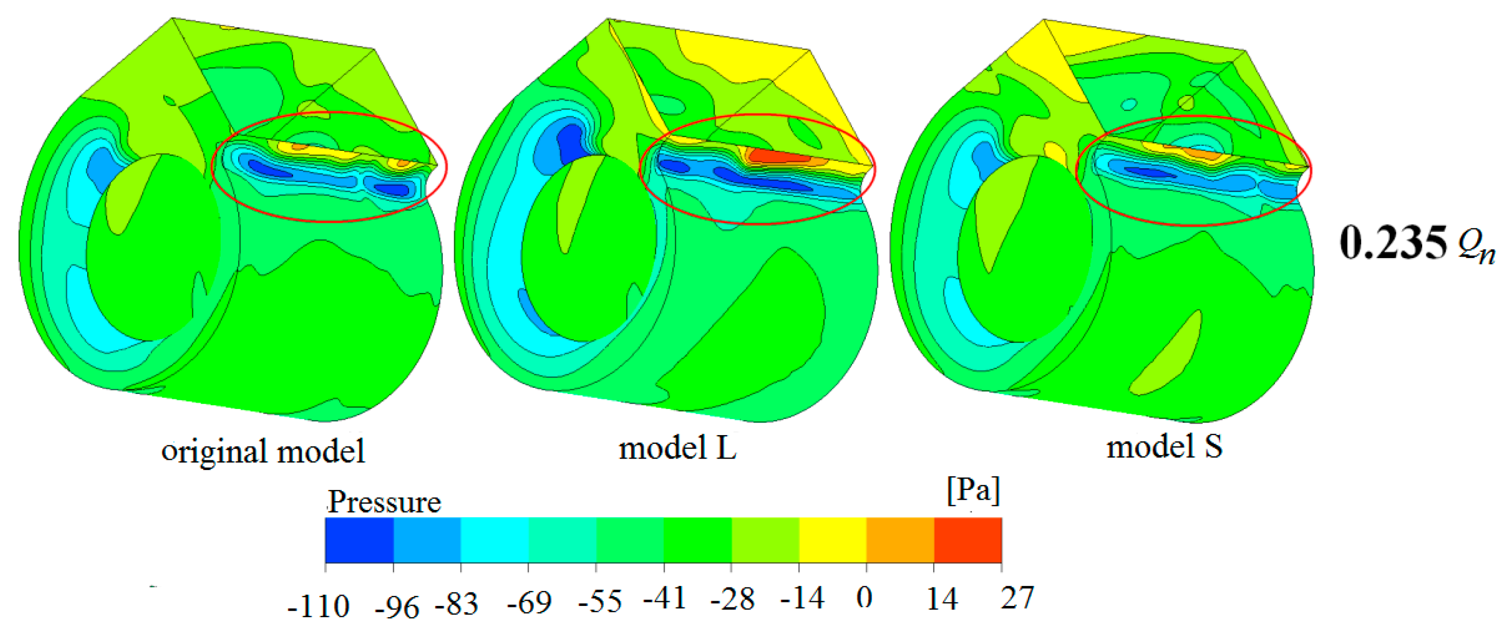
Figure 13 shows the static pressure distribution on the surface of the volute tongue at 0.235Qn. One can see that a low-pressure region and a high-pressure region appear on the surface of the volute tongue along the flow direction in each model at the condition of the lower flow rate, and the distribution range is large along the axial direction. For the model-L, the high-pressure region mainly locates at the middle part of tongue surface; the pressure value near middle part of tongue surface is obviously higher than that of the model-S and baseline model at 0.235Qn.
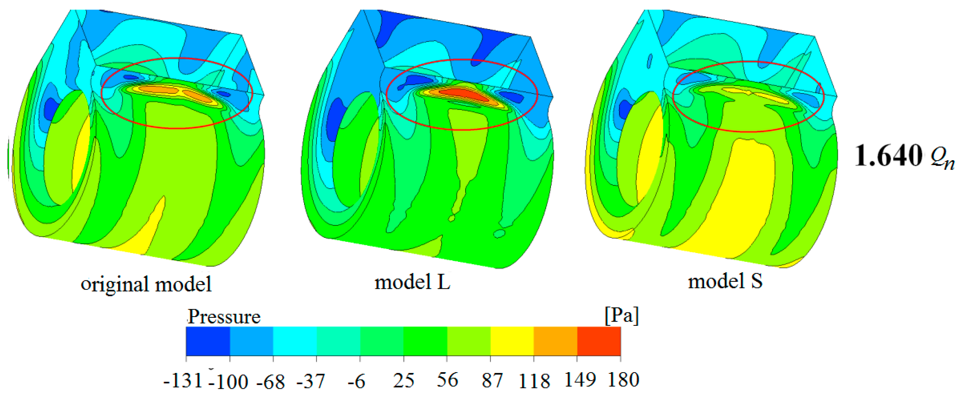
Figure 14 and Figure 15 show the static pressure distribution on the surface of the volute tongue at design points Qn and 1.64Qn, respectively. Plotted in Figure 14, it is observed that the low-pressure region disappears at design point Qn, and is replaced by a high-pressure region mainly in the middle of the volute tongue, which occupies about one third of the area. As shown in Figure 15, it is noted that the area of the high-pressure region on the middle of volute tongue surface increases at a high flow rate condition while the low-pressure region appears on both sides of the tongue.
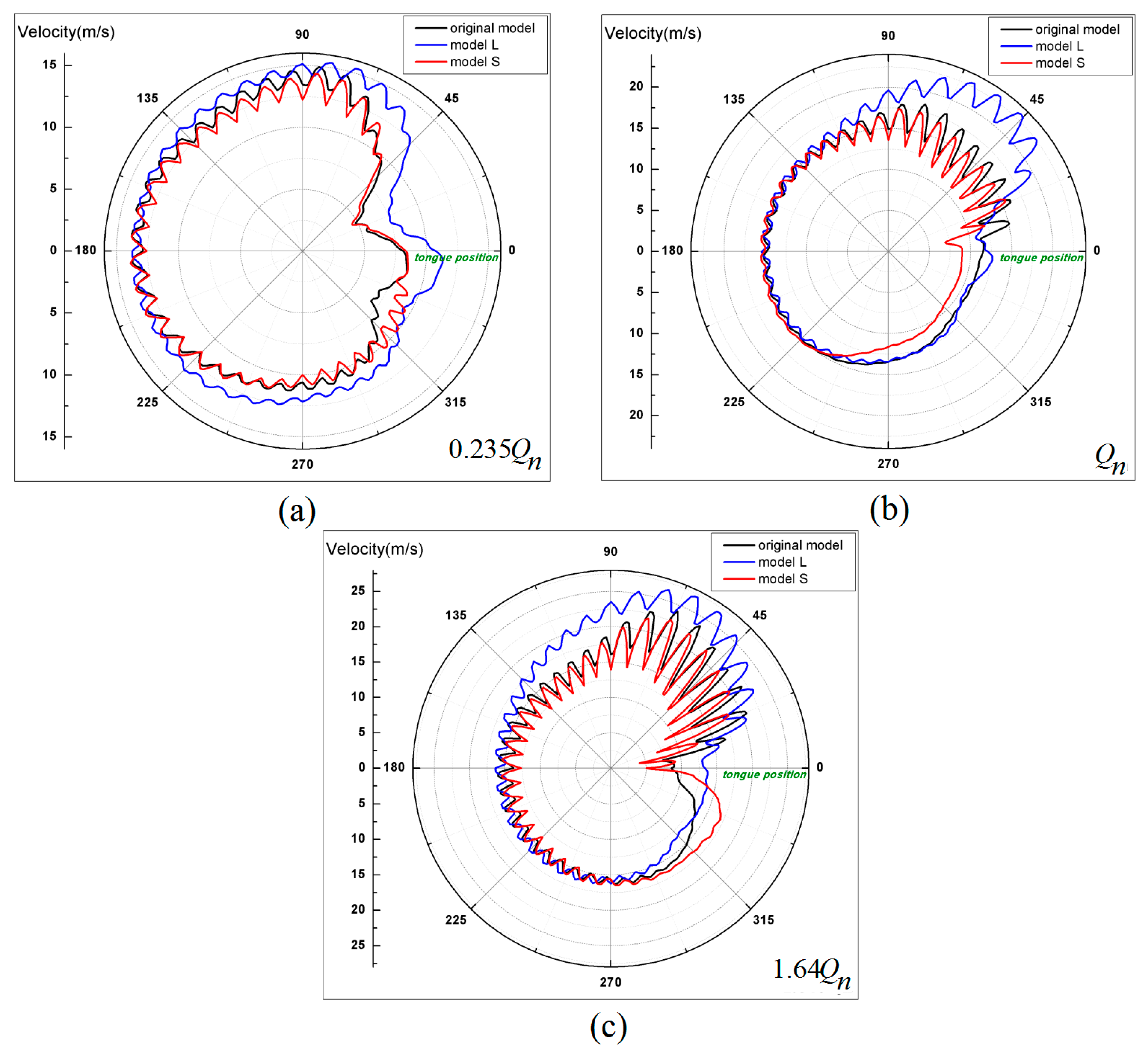
Figure 16 shows the velocity profile (along the circumferential direction) near the blade trailing edge of impeller exit for the baseline model, model-S and model-L at different flow rates. As shown in this figure, it is observed that at 0.235Qn, the velocity distribution at the outlet of each model impeller varies slightly and seemed uniform along the circumferential direction. Little difference appears for the peak velocity of each model; the velocity slowly decreases near the volute outlet and the volute tongue area. It is also obtained that at design rate (Qn) and high flow rate (1.640Qn), the velocity of all models greatly increases near the outlet of the volute and then rapidly decreases near the volute tongue, and the difference between the highest and the lowest velocity magnitude on the profile increases along the circumferential direction. The velocity of model-L is the highest near the volute outlet, but the amplitude of the velocity fluctuation is the smallest over the whole circumferential distance. In other words, the velocity profile (along the circumferential direction) near the blade trailing edge of the impeller exit obviously increases with the increase of the blade length at various flow rates. Nevertheless, the velocity amplitude of fluctuation decreases with the increase of the blade length.
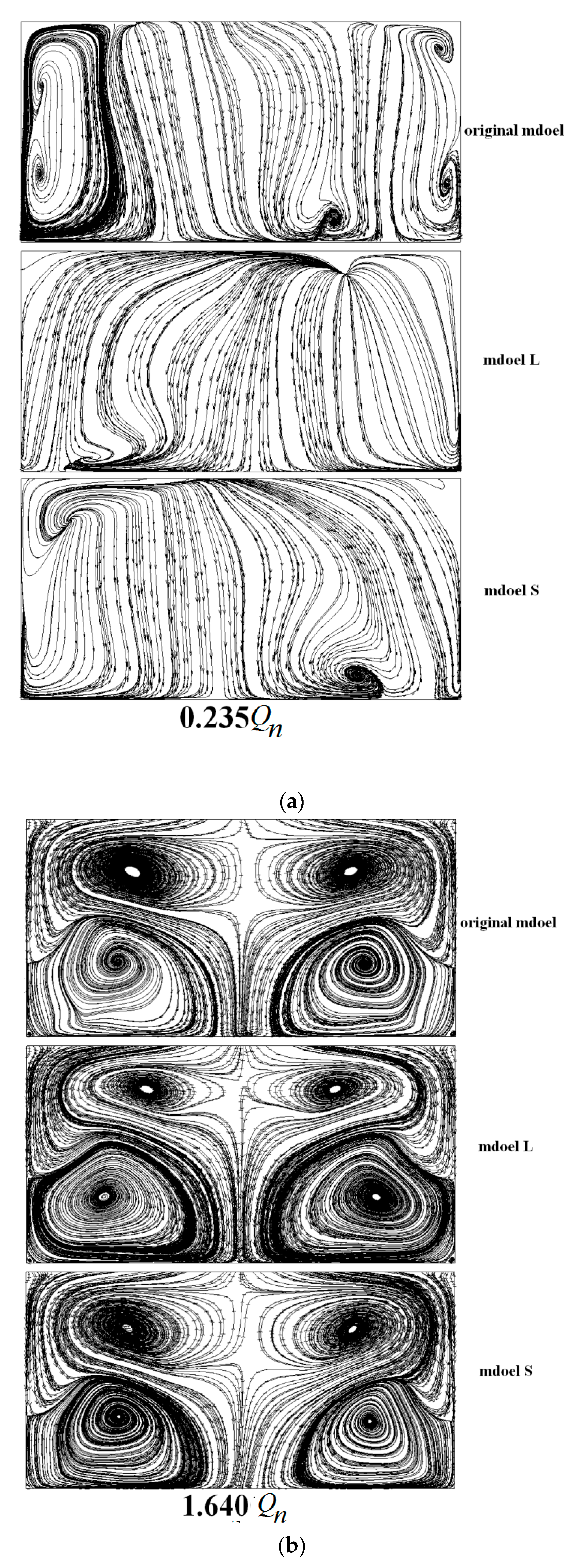
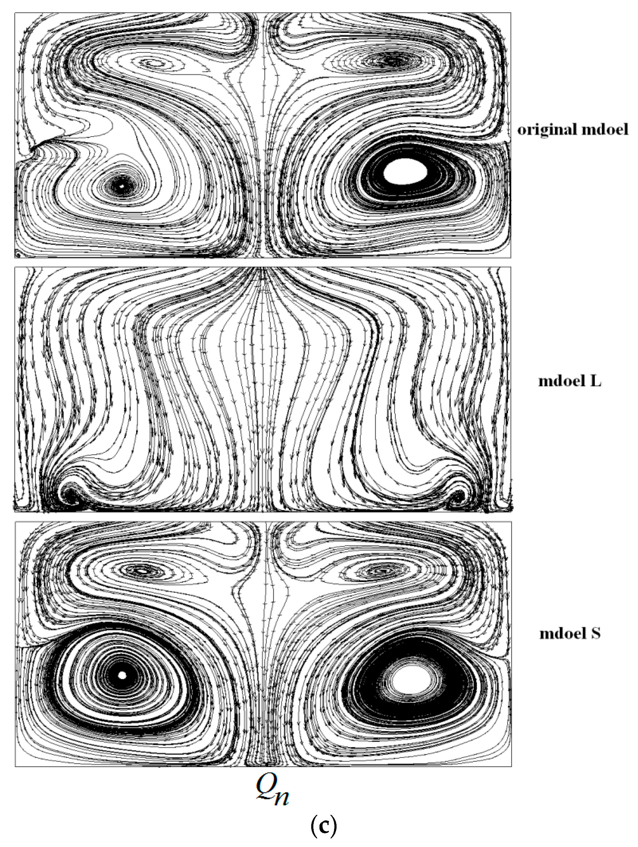
The streamline at the exit surface of the volute is shown in Figure 17. One can see that at a lower flow rate condition, a number of small vortices form on both sides of the volute exit in the baseline model, where one small vortex forms on the bottom of model-S and no small vortex forms in model-L, which indicates that the flow loss at the exit surface of volute for model-L is obviously lower than that of the baseline model. At design point, a number of secondary flows arise at the exit surface of the baseline model and model-S. However, no secondary flow occurs in model-L, which also indicates that the flow loss at the exit surface of the volute for model-L is obviously lower than that of the baseline model and model-S.
It is also obtained that the symmetry of streamline on the exit surface has been improved with the increase of the flow rate, and this also greatly promotes the development of secondary flow with the influence on the flow in the volute discharge.
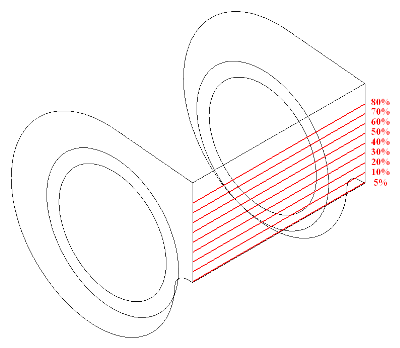
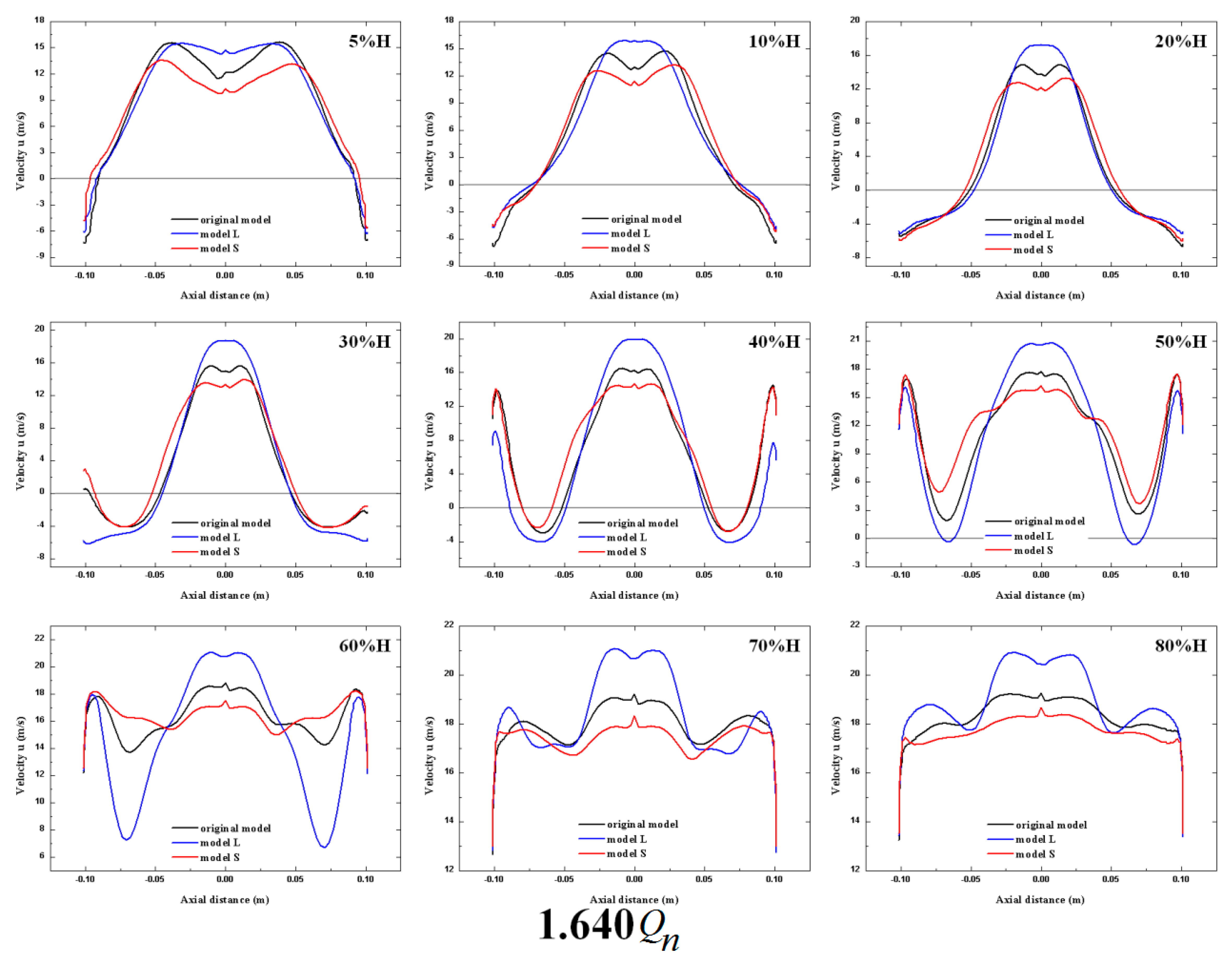
Figure 18 shows the nine sections of volute outlet from bottom to top. Figure 19 shows the velocity distribution along the height (from 5% H to 80% H) of the volute outlet at the design condition. Plotted in Figure 19, it is observed that at the design point, the backflow area of model-L is the largest in the middle and lower part of the volute outlet. The backflow area of the model-L is reduced to a minimum at 40% H and disappears completely at 50% H, while a small range of backflow occurs in the baseline model and the model-S. The backflow completely disappears in the middle and upper part of the volute outlet for all models. At a high flow rate condition, the backflow range of all models is close to the lower part of the volute outlet. With the increase of the outlet height, the backflow range of the baseline model and model-S decreases rapidly and disappears at 50% H, while a small range of backflow still occurs in the model-L, and the velocity gradient increases in the axial direction.
Figure 20 illustrates the velocity distribution along the height (from 5% H to 80% H) of volute outlet at the high flow rate condition (1.64Qn). The x-axis refers to the axial position and the y-axis refers to the velocity perpendicular to the volute outlet. The negative value of velocity (below the 0 scale line of the ordinate as shown in Figure 19) indicates that the backflow appears at this height of the volute outlet. The backflow at the volute outlet mainly converges at the low height region of the outlet, and the range of backflow gradually narrows and finally disappears with the increase of the height.
4.3. Performance Results of Numerical Simulations
The relevant parameters for the performance of the fan, i.e., output power, shaft power and total-to-total efficiency for the impeller flow field, are defined by
in which , , and denote the impeller torque, rate of flow, total pressure increases across the bell mouth and impeller, and the fan flow rate. The performance of the entire fan is calculated differently from calculation of the impeller. The is again evaluated by Equation (5), but is evaluated by integrating the torque from all the impeller blades. The lift-side total and static efficiency are defined by:
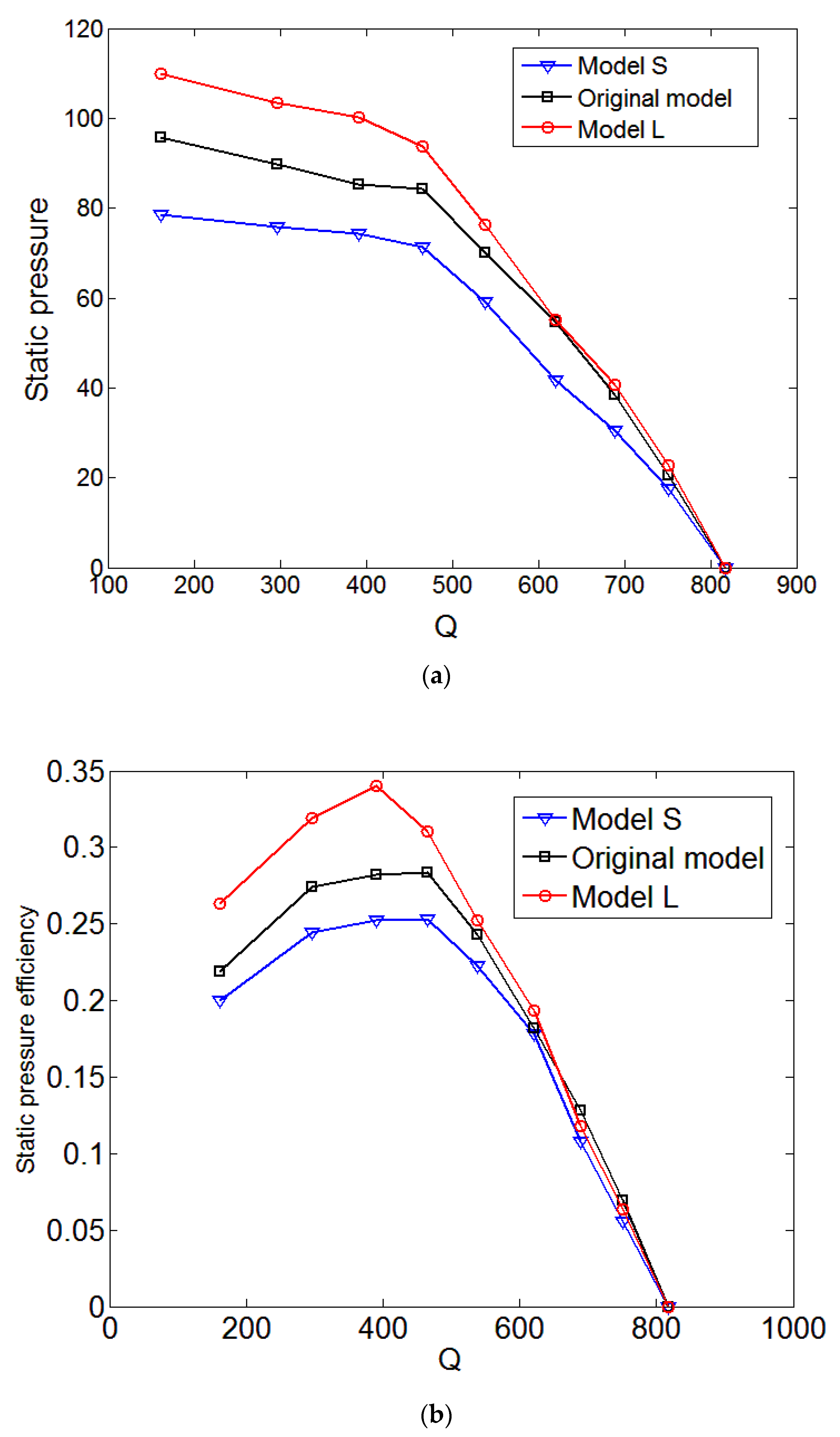
Figure 21 shows the static pressure and static pressure efficiency for various models obtained by steady numerical simulations. As shown in Figure 22, it is clearly observed that the static pressure and static pressure efficiency of model-L are obviously higher than that of model-S and the baseline model at the design flow rate, and the static pressure and static pressure efficiency of model-S are obviously lower than that of the baseline model at the design flow rate. The static pressure and static pressure efficiency obviously increases with the increase of the blade length of model-S, the baseline model and model-L at the design flow rate. It is also obtained that the static pressure value of the model-S is about 78 Pa, the static pressure value of the baseline model is about 82 Pa, and the static pressure value of the model-L is about 104 Pa. We can obtain that at the designed flow rate, the improved static pressure of the model-L rises as much as 23 Pa. It is further found that the static pressure efficiency of the baseline model is about 27.5%, and the static pressure efficiency of the model-L is about 33.5%, and also the improved static pressure efficiency of the model-L rises as much as 6% at design flow rates. Our work suggests that reducing the blade inlet angle (β1A > 60°) and improving the blade outlet angle (β2A < 175°) can provide a significant increase on the static pressure and the efficiency of static pressure, which improves the aerodynamic load of the forward multiblade fan to achieve the aim of energy conservation.
4.4. Performance Results of Experimental Test
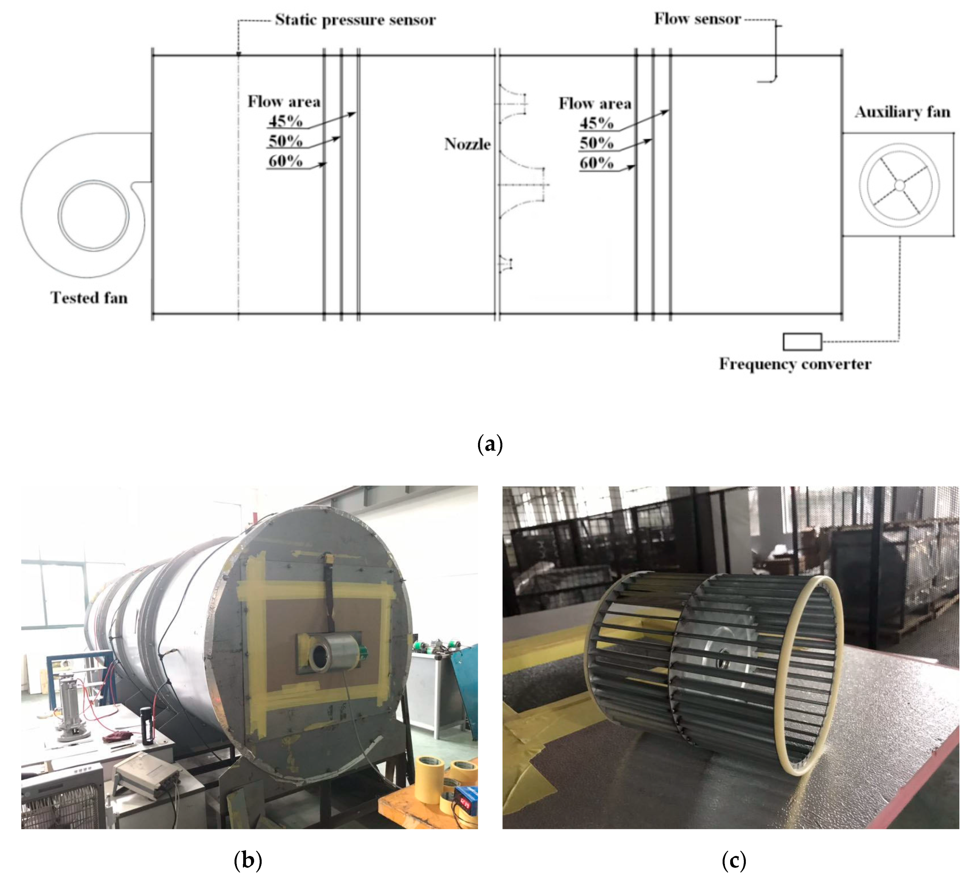
Figure 22 shows the performance measurement device of testing the centrifugal fan. Plotted in Figure 22, the centrifugal fan is mounted on the inlet of Yilida’s performance measurement device. At the outlet of the wind tunnel an auxiliary fan is mounted. The network of steady flow is mounted in the chamber to measure homogeneous flow. Multiple nozzles are implemented in the chamber. The details of the test rig are shown in Figure 22b. Figure 22c presents the impeller of model-L in experimental performance measurement.
The performance characteristics of the baseline model and model-L are performed on a chamber test rig. The performance data, such as static pressure, total pressure, static pressure efficiency and total pressure efficiency, are obtained at a range of flow rates. The measuring device for testing the centrifugal fan is manufactured by Air Movement and Control Association International (AMCA) standard. The centrifugal fan is placed at the entrance of the performance measuring device, and an auxiliary fan is placed at the outlet as shown in Figure 22. A steady flow network in the chamber can provide stable flow patterns for measurement. Pairs of nozzles are installed in the chamber to obtain various flow rates. A throttling device with an auxiliary fan to control the operating point of the testing centrifugal fan is used at the outlet of the test chamber.
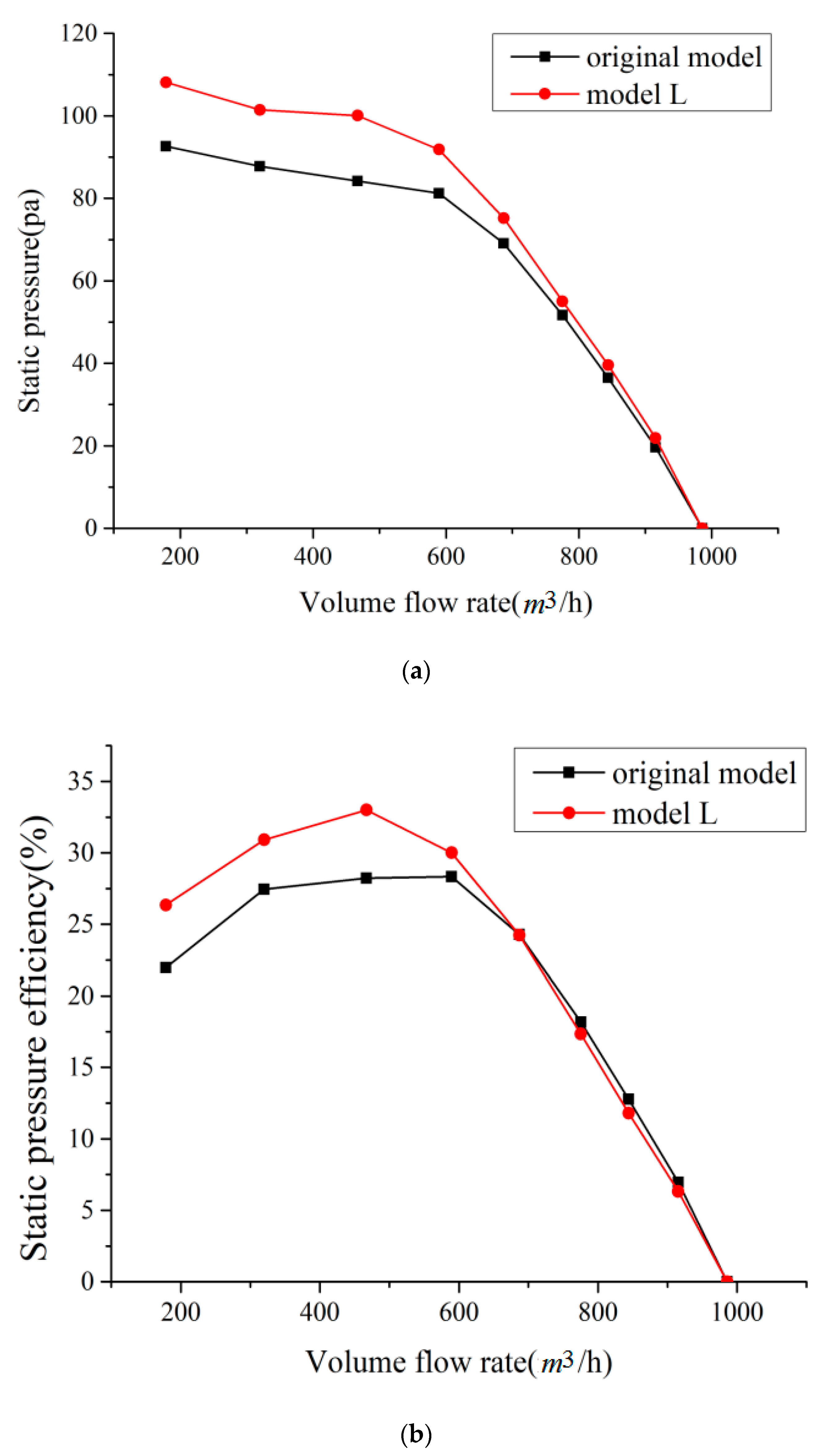
Figure 23 shows the static pressure and static pressure efficiency for the baseline model and model-L by experimental test. One can see that the static pressure and static pressure efficiency of model-L are obviously higher than that of the baseline model near the design flow rate. The static pressure value of the baseline model is about 82.5 Pa, and the static pressure value of the model-L is about 105 Pa. It is obvious that compared to the baseline model, the static pressure of the model-L rises as much as 22.5 Pa at the design flow rate. It is also obtained that the static pressure efficiency of the baseline model is about 26.4% (including efficiency of the motor), and the static pressure efficiency of the model-L is about 31.5% (including efficiency of the motor), thus the static pressure efficiency of the model-L rises as much as 5% at the design flow rate.
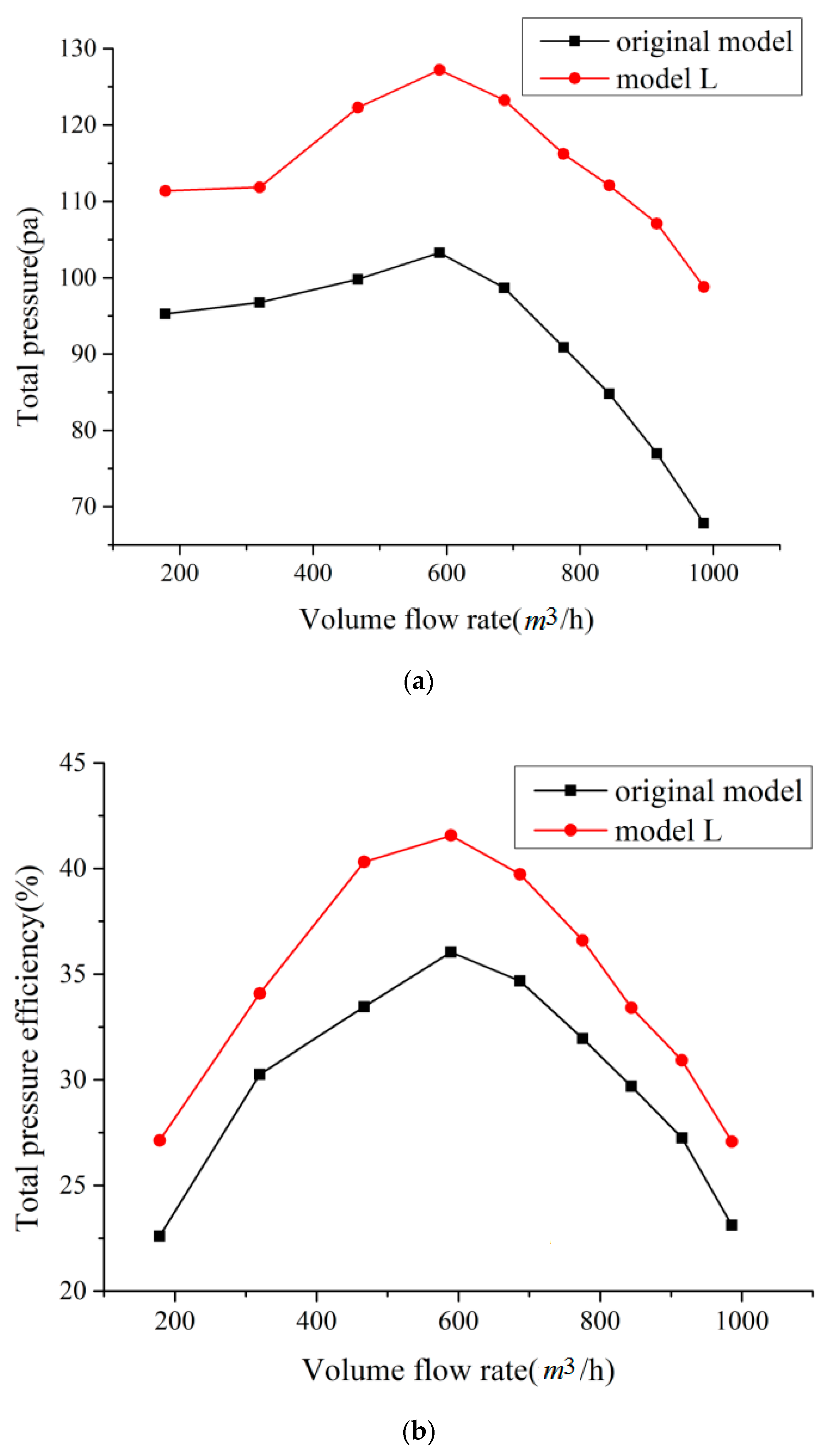
Figure 24 demonstrates the total pressure and total pressure efficiency for the baseline model and model-L by experimental test. The total pressure and total pressure efficiency of model-L are obviously higher than that of the baseline model at all flow rates. The total pressure value of the baseline model is about 101.5 Pa, and the total pressure value of the model-L is about 125.4 Pa, thus the static pressure of the model-L rises as much as 25 Pa compared with that of the baseline model.
It is also found that the total pressure efficiency of the baseline model is about 35.5% (including the efficiency of the motor), and the total pressure efficiency of the model-L is about 41.5% (including efficiency of the motor), thus the total pressure efficiency of the model-L rises as much as 6% at the design flow rate.
5. Conclusions
In this paper, the effects of single-arc blade profile length on the performance of a forward multiblade fan are presented and demonstrated. The internal complex flow characteristics of fans are investigated by numerical simulations by implementing the RANS turbulence model, and the performance of fans is studied by numerical simulations and experimental test. Several conclusions can be summarized as follows:
The gradient of the absolute velocity among the blades in model-L is clearly lower than that of the baseline model and model-S, and the gradient of the absolute velocity among the blades decreases in model-L, which brings about the size of the flow separation among the blades.
At the design point Qn, the area of turbulent kinetic energy at the inlet of the volute for model-L is smaller than that of the baseline model and model-S. The flow loss at the exit surface of the volute for model-L is obviously lower than that of the baseline model and model-S
Experimental results demonstrate that the static pressure of model-L rises as much as 22.5 Pa and 26.2%, while the static pressure efficiency of the model-L rises as much as 5% at the design flow rate. Meanwhile, the total pressure of the model-L rises as much as 25 Pa and 23.6%, and the total pressure efficiency of the model-L rises as much as 6% at the design flow rates.
It is found that a properly increasing blade working area provides a significant increasing on the static pressure, total pressure, the efficiency of static pressure and total pressure efficiency. The increase of the blade working area obviously improves the aerodynamic load of fans to achieve the purpose of energy conservation.
Author Contributions
The following statements could be used Y.W. and C.Y. conceived and designed the experiments; J.X. performed the experiments; W.C. and Z.W. analyzed the data; Z.Z. contributed reagents/materials/analysis tools; Y.W. wrote the paper.
Funding
This work was supported by the National Natural Science Foundation of China (11872337, 11902291 and U1709209), Natural Science Foundation of Zhejiang Province (LY18A020010), public welfare technology application research project of Zhejiang province (2017C31075), and Fundamental Research Funds of Zhejiang Sci-Tech University (2019Y004).
Acknowledgments
The authors appreciate sincerely the referees’ valuable comments and suggestions on our work.
Conflicts of Interest
The authors declare no conflict of interest.
References
- Cau, G.; Mandas, N.; Manfrida, N.; Nurzia, F. Measurements of primary and secondary flows in an industrial forward-curved centrifugal fan. ASME J. Turbomach. 1990, 112, 84–90. [Google Scholar] [CrossRef]
- Cao, S.; Chu, L. Experimental study on the matching between centrifugal impeller and volute. Chin. Fluid Mach. 1991, 10, 2–4. [Google Scholar]
- Wei, Y.K.; Yang, H.; Lin, Z.; Wang, Z.D.; Qian, Y.H. A novel two-dimensional coupled lattice Boltzmann model for thermal incompressible flows. Appl. Math. Comput. 2018, 339, 556–567. [Google Scholar] [CrossRef]
- Liang, H.; Li, Y.; Chen, J.X.; Xu, J.R. Axisymmetric lattice Boltzmann model for multiphase flows with large density ratio. Int. J. Heat Mass Transf. 2019, 130, 1189–1205. [Google Scholar] [CrossRef]
- Zhang, W.; Chen, X.P.; Yang, H.; Liang, H.; Wei, Y.K. Forced convection for flow across two tandem cylinders with rounded corners in a channel. Int. J. Heat Mass Transf. 2019, 130, 1053–1069. [Google Scholar] [CrossRef]
- Zhou, H.; Ca, G.B. Research of wall roughness effects based on Q criterion. Microfluid. Nanofluid. 2017, 21, 114–121. [Google Scholar] [CrossRef]
- Šístek, V. Corotational and Compressibility Aspects Leading to a Modification of the Vortex-Identification Q-Criterion. AIAA J. 2015, 53, 2406–2410. [Google Scholar]
- Gong, W.; Lv, W.; Xi, G.; Zhang, W. Experimental study on the velocity field near the tongue of a forward curved multi-blades centrifugal fan. Chin. J. Mech. Eng. 2005, 41, 166–171. [Google Scholar] [CrossRef]
- Velarde-Suárez, S.; Santolaria-Morros, C.; Ballesteros-Tajadura, R. Experimental study on the aeroacoustic behavior of a forward-curved blades centrifugal fan. ASME J. Fluid Eng. 1999, 121, 276–281. [Google Scholar] [CrossRef]
- Velarde-Suárez, S.; Ballesteros-Tajadura, R.; Santolaria-Morros, C.; Gonzalez-Perez, J. Unsteady flow pattern characteristics downstream of a forward-curved blades centrifugal fan. ASME J. Fluid Eng. 2001, 123, 265–270. [Google Scholar] [CrossRef]
- Younsi, M.; Bakir, F.; Kouidri, S.; Rey, R. Numerical and experimental study of unsteady flow in centrifugal fan. Proc. Inst. Mech. Eng. Part A J. Power Energy 2007, 221, 1025–1036. [Google Scholar] [CrossRef]
- Lin, S.; Huang, C. An integral experimental and numerical study of forward curved centrifugal fan. Exp. Fluid Sci. 2002, 26, 421–434. [Google Scholar] [CrossRef]
- Lun, Y.X.; Lin, L.M.; Zhu, Z.C.; Wei, Y.K. Effects of Vortex Structure on Performance Characteristics of a Multiblade Fan with Inclined tongue. Proc. Inst. Mech. Eng. Part A J. Power Energy 2019, 233, 1007–1021. [Google Scholar] [CrossRef]
- Montazerin, N.; Damangir, A.; Mirian, S. A new concept for squirrel cage fan inlet. J. Power Energy 1998, 212, 343–349. [Google Scholar] [CrossRef]
- Montazerin, N.; Damangir, A.; Mirzaie, H. Inlet induced flow in squirrel-cage fans. J. Power Energy 2000, 214, 243–253. [Google Scholar] [CrossRef]
- Bayomi, N.N.; Osman, A.M. Effect of inlet straighteners on centrifugal fan performance. Energy Convers. Manag. 2006, 47, 3307–3318. [Google Scholar] [CrossRef]
- Zheng, X.; Lin, Z.; Xu, B.Y. Thermal conductivity and sorption performance of nano-silver powder/FAPO-34 composite fin. Appl. Therm. Eng. 2019, 160, 114055. [Google Scholar] [CrossRef]
- Hosangadi, A.; Lee, R.A.; York, B.J.; Sinha, N.; Dash, S.M. Upwind Unstructured Scheme for Three-Dimensional Combusting Flows. J. Propul. Power 1996, 12, 494–502. [Google Scholar] [CrossRef]
- Hosangadi, A.; Lee, R.A.; Cavallo, P.A.; Sinha, N.; York, B.J. Hybrid, Viscous, Unstructured Mesh Solver for Propulsive Applications. In Proceedings of the AIAA 34th JPC, Cleveland, OH, USA, 13–15 July 1998; Volume 98, p. 3153. [Google Scholar]
- Lee, Y.T.; Mulvihill, L.; Coleman, R.; Ahuja, V.; Hosangadi, A.; Birkbeck, R.; Becnel, A.; Slipper, M. LCAC Lift Fan Redesign and CFD Evaluation. Nav. Surf. Warf. Cent. Rep. 2007, 23, 112–119. [Google Scholar]
- Wang, C.; Hu, B.; Zhu, Y.; Wang, X.; Luo, C.; Cheng, L. Numerical study on the gas-water two-phase flow in the self-priming process of self-priming centrifugal pump. Processes 2019, 7, 330. [Google Scholar] [CrossRef]
- Zhang, S.F.; Li, X.J.; Hu, B.; Liu, Y.; Zhu, Z.C. Numerical investigation of attached cavitating flow in thermo-sensitive fluid with special emphasis on thermal effect and shedding dynamics. Int. J. Hydrog. Energy 2019, 44, 3170–3184. [Google Scholar] [CrossRef]
- Li, X.J.; Jiang, Z.W.; Zhu, Z.C.; Si, Q.R.; Li, Y. Entropy generation analysis for the cavitating head-drop characteristic of a centrifugal pump. Proc. Inst. Mech. Eng. Part C J. Mech. Eng. Sci. 2018, 232, 4637–4646. [Google Scholar] [CrossRef]
- Liu, Q.; Ye, J.H.; Zhang, G.; Lin, Z.; Xu, H.; Jin, H.; Zhu, Z. Study on the metrological performance of a swirlmeter affected by flow regulation with a sleeve valve. Flow Meas. Instrum. 2019, 67, 83–94. [Google Scholar] [CrossRef]
- Xu, H.; Cantwell, C.D.; Monteserin, C.; Eskilsson, C.; Engsig-Karupet, A.P.; Sherwin, S.J. Spectral/hp element methods: Recent developments, applications, and perspectives. J. Hydrodyn. 2018, 30, 1–22. [Google Scholar] [CrossRef] [Green Version]
- Xu, H.; Mughal, S.M.; Gowree, E.R.; Atkin, C.J.; Sherwin, S.J. Destabilisation and modification of Tollmien–Schlichting disturbances by a three-dimensional surface indentation. J. Fluid Mech. 2017, 819, 592–620. [Google Scholar] [CrossRef]
- Zhang, W.; Li, X.J.; Zhu, Z.C. Quantification of wake unsteadiness for low-Re flow across two staggered cylinders. Proc. Inst. Mech. Eng. Part C J. Mech. Eng. Sci. 2019. [Google Scholar] [CrossRef]
- Xu, H.; Sherwin, S.J.; Hall, P.; Wu, X. The behaviour of Tollmien–Schlichting waves undergoing small-scale localised distortions. J. Fluid Mech. 2016, 792, 499–525. [Google Scholar] [CrossRef]
- Xu, H.; Lombard, J.E.; Sherwin, S.J. Influence of localised smooth steps on the instability of a boundary layer. J. Fluid Mech. 2017, 817, 138–170. [Google Scholar] [CrossRef] [Green Version]
- Wang, C.; Shi, W.; Wang, X.; Jiang, X.; Yang, Y.; Li, W.; Zhou, L. Optimal design of multistage centrifugal pump based on the combined energy loss model and computational fluid dynamics. Appl. Energy 2017, 187, 10–26. [Google Scholar] [CrossRef]
- Liu, Q.; Ye, J.; Zhang, G.; Lin, Z.; XU, H.; Zhu, Z. Metrological performance investigation of swirl flow meter affected by vortex inflow. J. Mech. Sci. Technol. 2019, 33, 2671–2680. [Google Scholar] [CrossRef]
- Chen, X.P.; Li, X.P.; Dou, H.S.; Zhu, Z.C. Effects of variable specific heat on energy transfer in a high-temperature supersonic channel flow. J. Turbul. 2018, 19, 365–389. [Google Scholar] [CrossRef]
- Chen, X.P.; Li, X.L.; Zhu, Z.C. Effects of dimensional wall temperature on velocity-temperature correlations in supersonic turbulent channel flow of thermally perfect gas. Sci. China Phys. Mech. Astron. 2019, 62, 064711–064719. [Google Scholar] [CrossRef]
- Yang, H.; Zhang, W.; Zhu, Z.C. Unsteady mixed convection in a square enclosure with an inner cylinder rotating in a bi-directional and time-periodic mode. Int. J. Heat Mass Transf. 2019, 136, 563–580. [Google Scholar] [CrossRef]
Figure 1.
Example of double inlet radial fan with forward curved blade.

Figure 2.
Blade shape of test cases and geometrical parameters of the baseline model.

Figure 3.
Domain composition: Inlet left (a), inlet right (b), impeller (c), volute (d) and outlet (e). The domain interface is colored in deep red.
Figure 3.
Domain composition: Inlet left (a), inlet right (b), impeller (c), volute (d) and outlet (e). The domain interface is colored in deep red.

Figure 4.
Detail of the numerical mesh and Static pressure at different number of grids. (a) numerical meshes of the volute; (b) static pressure at different number of grids.
Figure 4.
Detail of the numerical mesh and Static pressure at different number of grids. (a) numerical meshes of the volute; (b) static pressure at different number of grids.


Figure 5.
Comparison of static pressure and the static pressure efficiency between numerical results and experimental results. (a) curve of static pressure -flow (b) curve of static pressure efficiency-flow.
Figure 5.
Comparison of static pressure and the static pressure efficiency between numerical results and experimental results. (a) curve of static pressure -flow (b) curve of static pressure efficiency-flow.

Figure 6.
Different heights within the impeller.

Figure 7.
Absolute velocity at different heights within the impeller at 0.235Qn.

Figure 8.
Absolute velocity at different heights within the impeller at Qn.

Figure 9.
Absolute velocity at different heights within the impeller at 1.640Qn.

Figure 10.
Distribution of turbulence kinetic energy of the impeller at 0.235Qn.

Figure 11.
Distribution of turbulence kinetic energy of the impeller at Qn.

Figure 12.
Distribution of turbulence kinetic energy of the impeller at 1.640Qn.

Figure 13.
Static pressure distribution on the surface of the volute tongue at 0.235Qn.

Figure 14.
Static pressure distribution on the surface of the volute tongue at Qn.

Figure 15.
Static pressure distribution on the surface of the volute tongue at 1.640Qn.

Figure 16.
Velocity profile above the impeller. (a) velocity profile at 0.235 ; (b) velocity profile at ; (c) velocity profile at 1.64 .
Figure 16.
Velocity profile above the impeller. (a) velocity profile at 0.235 ; (b) velocity profile at ; (c) velocity profile at 1.64 .

Figure 17.
The streamline on the exit surface of volute. (a) at 0.235 ; (b) at 1.64 ; (c) at .


Figure 18.
Section of volute outlet from bottom to top.

Figure 19.
Velocity distribution along the height of volute outlet at the design condition.

Figure 20.
Velocity distribution along the height of volute outlet at 1.64Qn.

Figure 21.
Static pressure and static pressure efficiency of different model (Q, m3/h). (a) static pressure-flow; (b) static pressure efficiency-flow.
Figure 21.
Static pressure and static pressure efficiency of different model (Q, m3/h). (a) static pressure-flow; (b) static pressure efficiency-flow.

Figure 22.
Experimental device and impeller model. (a) two-dimensional cross-section of performance measurement device; (b) on-site testing equipment; (c)impeller of model-L in experimental performance measurement.
Figure 22.
Experimental device and impeller model. (a) two-dimensional cross-section of performance measurement device; (b) on-site testing equipment; (c)impeller of model-L in experimental performance measurement.

Figure 23.
Experimental static pressure and static pressure efficiency for the baseline model and model-L. (a) static pressure-flow; (b) static pressure efficiency-flow.
Figure 23.
Experimental static pressure and static pressure efficiency for the baseline model and model-L. (a) static pressure-flow; (b) static pressure efficiency-flow.

Figure 24.
Experimental total pressure and total pressure efficiency for baseline model and model-L. (a) total pressure-flow; (b) total pressure efficiency-flow.
Figure 24.
Experimental total pressure and total pressure efficiency for baseline model and model-L. (a) total pressure-flow; (b) total pressure efficiency-flow.


Table 1.
Blade inlet angle and blade outlet angle of the three models.
| Baseline Model | Model-S | Model-L | |
|---|---|---|---|
| Blade inlet angle (β2A) | 84.83° | 91.27° | 71.34° |
| Blade outlet angle (β1A) | 152.36° | 146.69° | 170.13° |
© 2019 by the authors. Licensee MDPI, Basel, Switzerland. This article is an open access article distributed under the terms and conditions of the Creative Commons Attribution (CC BY) license (http://creativecommons.org/licenses/by/4.0/).
Share and Cite
MDPI and ACS Style
Wei, Y.; Ying, C.; Xu, J.; Cao, W.; Wang, Z.; Zhu, Z. Effects of Single-arc Blade Profile Length on the Performance of a Forward Multiblade Fan. Processes 2019, 7, 629. https://doi.org/10.3390/pr7090629
AMA Style
Wei Y, Ying C, Xu J, Cao W, Wang Z, Zhu Z. Effects of Single-arc Blade Profile Length on the Performance of a Forward Multiblade Fan. Processes. 2019; 7(9):629. https://doi.org/10.3390/pr7090629
Chicago/Turabian StyleWei, Yikun, Cunlie Ying, Jun Xu, Wenbin Cao, Zhengdao Wang, and Zuchao Zhu. 2019. "Effects of Single-arc Blade Profile Length on the Performance of a Forward Multiblade Fan" Processes 7, no. 9: 629. https://doi.org/10.3390/pr7090629
Note that from the first issue of 2016, this journal uses article numbers instead of page numbers. See further details here.