A Hidden Anomaly in the Binary Mixture Natural Convection Subject to Flux Boundary Conditions

Abstract

The problem of natural convection in a binary mixture subject to realistic boundary conditions of imposed zero mass flux on the solid walls shows solutions that might lead to unrealistic negative values of the mass fraction (or solute concentration). This anomaly is being investigated in this paper, and a possible way of addressing it is suggested via a mass-fraction-dependent thermodiffusion coefficient that can have negative values in regions of low mass fractions.

1. Introduction

Setting specified arbitrary values of the mass fraction (or solute concentration) on the boundaries of a binary mixture is extremely difficult, if not impossible, to accomplish experimentally. A more realistic boundary condition for the mass fraction (solute concentration) is a zero-flux boundary condition accounting for thermodiffusion via thermophoresis (Soret effect). Brand et al. [1] also indicated that varying the temperature and mass fraction (concentration) gradients independently is “… a condition, which is difficult to meet in practice due to cross-coupling (thermodiffusion) between the gradients, which exist in real fluids”.

A binary fluid mixture is a general form of a mixture consisting typically of two-phases with one phase being fluid and the other phase being either another fluid (miscible, e.g., water and alcohol, or immiscible like emulsions, e.g., oil in water), or solid particles either dissolved in the fluid (solution, e.g., salt in water, in this case, this will be one single-phase), or suspended in the fluid (colloids, e.g., aluminum powder in water, aerosols in the air). Natural convection in a binary fluid mixture placed between two vertical walls and differentially heated from the sides is being considered. The extreme difficulty or even impossibility in setting specified values for the mass fraction (solute concentration) on the boundaries led to applying zero mass flux boundary conditions on these walls combined with the thermodiffusion flux. The thermal boundary conditions are of a constant heating heat flux on one wall and a constant cold (ambient) temperature on the other wall. Note that it is also extremely difficult to apply in practice a cooling heat flux boundary condition, while a heating heat flux can easily be applied by taping a film of electrically conducting material and passing an electric current through it. The Ohm’s heating in the film will produce the required heat flux into the fluid. Both the Soret (Bird et al. [2]) as well as the Dufour effects are being considered. The Dufour effect is negligibly small in liquids, but it is substantially strong in gases [3,4,5,6,7].

The mass flux that includes the Soret effect of thermodiffusion is typically represented in the form [4,8,9,10,11,12,13,14]:

$${\mathit{j}}_{*}=-D_{m*}{\nabla }_{*}{C}_{*}-C_{*}\left(1-C_{*}\right)D_{T*}{\nabla }_{*}{T}_{*},$$

(1)

where ${\mathit{j}}_{*}$ is the species mass flux, $C_{*}$ is the mass fraction, $T_{*}$ is temperature, $D_{m*}$ is the molecular diffusivity arising from Fick’s law of diffusion, and $D_{T*}$ is the thermodiffusion coefficient arising due to the Soret effect (thermophoresis). The argument for introducing the coefficient $C_{*}\left(1-C_{*}\right)$ is that it forces the mass flux to be zero when the mass fraction is zero, $C_{*}=0$, or when the mass fraction is one $C_{*}=1$. This formulation in Equation (1) excludes solutions of a component dissolved in a fluid, such as salt in water, as then the units in Equation (1) are incompatible and need correction to account for the latter. In addition, a common approximation is to set the values of $C_{*}$ in this coefficient equal to a constant $C_o$, leading to:

$${\mathit{j}}_{*}=-D_{m*}{\nabla }_{*}{C}_{*}-C_o\left(1-C_o\right)D_{T*}{\nabla }_{*}{T}_{*}.$$

(2)

The subscripts * and o identify dimensional variables and constants, while the quantities without these subscripts are dimensionless. In addition, the subscript o represents dimensional reference values.

There has been an extensive experimental effort in order to evaluate the thermodiffusion coefficient [4,8,9,10,11,12,13,14,15,16,17]. Experimental results aimed at evaluating the thermodiffusion coefficient $D_{T*}$ have identified that its value can become negative in some cases [4,8,9,10,11,12,14], apparently for small mass fractions of the lighter component. Madriaga et al. [11] found experimentally that the thermodiffusion coefficient is composition-dependent and measured this dependence. Costesèque et al. [13] indicate that the thermodiffusion coefficient is also temperature-dependent, and Geelhoed et al. [8], Putnam et al. [17], and Dhur and Braun [18] show experimental results identifying negative thermodiffusion coefficient values at lower temperatures (between 5 °C and 40 °C). Mojtabi et al. [19] also considered a temperature-dependent negative thermodiffusion coefficient in their analysis of the onset of natural convection.

The present paper shows that using a constant thermodiffusion coefficient $D_{T*}$ in the problem of natural convection of binary mixtures in a vertical fluid layer subject to differential heating leads to unrealistic negative values of mass fraction when flux boundary conditions are being used. As a remedy, it is suggested that a mass-fraction-dependent thermodiffusion coefficient, which can take negative values, is to be used in order to prevent this anomaly. While the latter transforms the diffusion terms and introduces a nonlinearity, it will be shown that it is not this nonlinearity that resolves the anomaly as suggested by Gorban et al. [20], but rather the specific characteristics of the thermodiffusion coefficient, which weakens or even changes the direction of the Soret effect in places where the mass fraction is low.

2. Problem Formulation

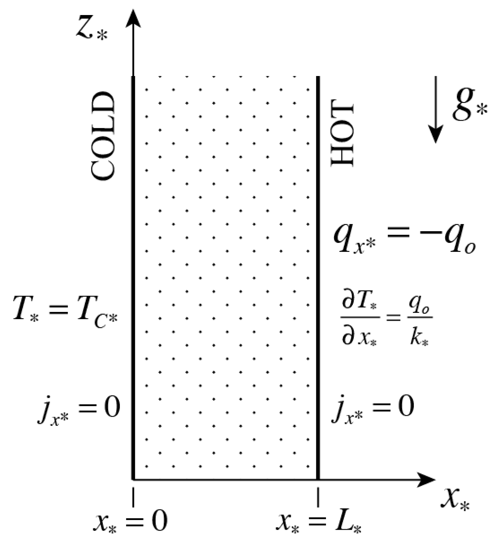
A binary mixture consisting of a vertical tall, fluid layer, having suspended (or dissolved) particles distributed within, is heated by a constant heat flux $q_o>0$ on one of its sides and exposed to a constant low temperature on the other side, as presented graphically in Figure 1. Mass cannot cross the solid boundaries at $x_{*}=0$ and $x_{*}=L_{*}$, and therefore, the mass flux of the suspended particles (or of the solute) is zero on these boundaries. The mass flux within the binary mixture is driven by the Soret effect due to the temperature gradients. The Soret effect for positive values of the thermodiffusion coefficient manifests itself by producing a mass flux in the direction down the temperature gradient, i.e., causing suspended particles to move from hot to cold regions.

The mass flux of the suspended particles (or of the solute) ${\mathit{j}}_{*}$ is represented by a combination of the Fick’s law flux and a Soret flux in the form:

$${\mathit{j}}_{*}=-D_{m*}{\nabla }_{*}{C}_{*}-C_o{D}_{T*}{\nabla }_{*}{T}_{*},$$

(3)

where, $D_{m*}$ carries units of ${\mathrm{m}}^2/\mathrm{s}$, and $D_{T*}$ is in units of ${\mathrm{m}}^2/(\mathrm{s}\hspace{0.17em}\mathrm{K})$.

The heat flux ${\mathit{q}}_{*}$ is a combination of a Fourier law heat flux and a DuFour flux in the form:

$${\mathit{q}}_{*}=-k_{*}{\nabla }_{*}{T}_{*}-\frac{{\rho }_o{T}_o{D}_{T*}}{c_{s*}}{\nabla }_{*}{C}_{*},$$

(4)

where $k_{*}$ is the thermal conductivity of the mixture, $T_o$ and ${\rho }_o$ are dimensional reference values of mixture temperature and density, respectively, and $c_{s*}$ is the mass fraction (concentration) susceptibility, carrying units of ${\mathrm{s}}^2/{\mathrm{m}}^2$ in the case suspensions, and $\mathrm{k}\mathrm{g}/(\mathrm{m}\hspace{0.17em}{\mathrm{s}}^2)$ in the case of solutions when the units of $C_{*}$ are $\mathrm{k}\mathrm{g}/{\mathrm{m}}^3$.

The energy and mass balance equations are:

$${\rho }_o{c}_{p*}\left[\frac{\partial \hspace{0.17em}{T}_{*}}{\partial \hspace{0.17em}{t}_{*}}+{\mathit{V}}_{*}·{\nabla }_{*}T\right]=-{\nabla }_{*}·{\mathit{q}}_{*},$$

(5)

$$\frac{\partial \hspace{0.17em}{C}_{*}}{\partial \hspace{0.17em}{t}_{*}}+{\mathit{V}}_{*}·{\nabla }_{*}C=-{\nabla }_{*}·{\mathit{j}}_{*},$$

(6)

respectively, where $c_{p*}={\left(\partial h_{*}/\partial T_{*}\right)}_{p*}$ is the specific heat capacity at constant pressure, while $h_{*}$ is the specific enthalpy, and ${\mathit{V}}_{*}=u_{*}\hspace{0.17em}{\widehat{e}}_x+{\mathrm{v}}_{*}{\widehat{e}}_y+w_{*}\hspace{0.17em}{\widehat{e}}_z$ is the velocity vector, while ${\widehat{e}}_x,\hspace{0.17em}{\widehat{e}}_y,\hspace{0.17em}{\widehat{e}}_z$ are unit vectors in the $x_{*},y_{*},$ and $z_{*}$ directions, respectively. Dividing Equation (5) by the constant product ${\rho }_o{c}_{p*}$ and substituting Equation (4) in the resulting equation, and Equation (3) in Equation (6) yields:

$$\frac{\partial \hspace{0.17em}{T}_{*}}{\partial \hspace{0.17em}{t}_{*}}+V_{*}·{\nabla }_{*}T={\alpha }_{*}\hspace{0.17em}{\nabla }_{*}^2{T}_{*}+\frac{T_o{D}_{T*}}{c_{s*}\hspace{0.17em}{c}_{p*}}\hspace{0.17em}{\nabla }_{*}^2{C}_{*},$$

(7)

$$\frac{\partial \hspace{0.17em}{C}_{*}}{\partial \hspace{0.17em}{t}_{*}}+{\mathit{V}}_{*}·{\nabla }_{*}C=D_{m*}{\nabla }_{*}^2{C}_{*}+C_o{D}_{T*}{\nabla }_{*}^2{T}_{*},$$

(8)

where ${\alpha }_{*}=k_{*}/{\rho }_o{c}_{p*}$ is the thermal diffusivity. The fluid flow is governed by the Navier–Stokes equations for an incompressible fluid via the continuity and momentum equations:

$${\nabla }_{*}·{\mathit{V}}_{*}=0,$$

(9)

$${\rho }_o\left[\frac{\partial \hspace{0.17em}{\mathit{V}}_{*}}{\partial \hspace{0.17em}{t}_{*}}+\left({\mathit{V}}_{*}·{\nabla }_{*}\right){\mathit{V}}_{*}\right]=-{\nabla }_{*}{p}_{*}+{\mu }_{*}{\nabla }_{*}^2{\mathit{V}}_{*}+{\rho }_{*}{g}_{*}{\widehat{e}}_g,$$

(10)

where $p_{*}$ is pressure, ${\mu }_{*}$ is the dynamic viscosity, $g_{*}$ is the scalar value of the acceleration due to gravity, ${\widehat{e}}_g$ is a unit vector in the direction of the acceleration due to gravity, and ${\rho }_{*}$ is the mixture’s density expressed as a linear approximation in the form:

$${\rho }_{*}={\rho }_o\left[1-{\beta }_{T*}\left(T_{*}-T_o\right)+{\beta }_{C*}{C}_{*}\right],$$

(11)

where ${\beta }_{T*}=-\left(\partial {\rho }_{*}/\partial T_{*}\right)/{\rho }_o$ and ${\beta }_{C*}=\left(\partial {\rho }_{*}/\partial C_{*}\right)/{\rho }_o$ are thermal expansion and mass fraction contraction coefficients, respectively. The Boussinesq approximation [21] was used in presenting the energy, mass transfer, continuity and momentum equations in the form (7), (8), (9), (10). Equation (11) is not part of the Boussinesq approximation, but rather a linear approximation that follows the former. The boundary conditions applicable to the vertical layer presented in Figure 1 are as follows:

$$x_{*}=0:\hspace{0.17em}\hspace{0.17em}{T}_{*}=T_{C*}\hspace{0.17em},\hspace{0.17em}\hspace{0.17em}\hspace{0.17em}{j}_{x*}=0\hspace{0.17em},\hspace{0.17em}\hspace{0.17em}\hspace{0.17em}{\mathit{V}}_{*}=0,$$

(12)

$$x_{*}=L_{*}:\hspace{0.17em}\hspace{0.17em}\frac{\partial T_{*}}{\partial x_{*}}=\frac{q_o}{k_{*}}\hspace{0.17em},\hspace{0.17em}\hspace{0.17em}\hspace{0.17em}{j}_{x*}=0\hspace{0.17em},\hspace{0.17em}\hspace{0.17em}\hspace{0.17em}{\mathit{V}}_{*}=0,$$

(13)

where $q_o>0$ is the heat flux imposed on the right wall.

The governing Equations (7)–(11) and boundary conditions (12), (13) are being converted into a dimensionless form by using as scales for density, length, velocity, time, pressure, temperature difference, and mass fraction, the reference value of density ${\rho }_o$, a characteristic length as the gap between the vertical walls $L_{*}$, a characteristic velocity ${\alpha }_{*}/L_{*}$, a characteristic time $L_{*}^2/{\alpha }_{*}$, a characteristic pressure ${\mu }_{*}{\alpha }_{*}/L_{*}^2$, a characteristic temperature difference $\Delta T_{ch}=q_o{L}_{*}/k_{*}$, and a reference value of the mass fraction $C_o$, respectively (also $T_o=T_{C*}$ in Equation (11)). The heat flux is also converted into a dimensionless form by using $q_o$ as a characteristic heat flux, leading to $q=q_{*}/q_o$, and the mass flux is converted in the form $j=j_{*}{L}_{*}/(D_m{C}_o)$. Consequently $\left(x,y,z\right)=\left(x_{*},y_{*},z_{*}\right)/L_{*}$, $t=t_{*}{\alpha }_{*}/L_{*}^2$, $V={\mathit{V}}_{*}{L}_{*}/{\alpha }_{*}$, $p=p_{*}{L}_{*}^2/{\mu }_{*}{\alpha }_{*}$, $\rho ={\rho }_{*}/{\rho }_o$, $T=\left(T_{*}-T_{C*}\right)k_{*}/\left(q_o{L}_{*}\right)$, $C=C_{*}/C_o$. The value of $C_o$ is the average mass fraction of the suspension. Equations (3), (4) and (7)–(11) converted into a dimensionless form become:

$$j=-\nabla C-So\hspace{0.17em}\nabla T,$$

(14)

$$q=-\nabla T-Du\hspace{0.17em}\nabla C,$$

(15)

$$\frac{\partial \hspace{0.17em}T}{\partial \hspace{0.17em}t}+V·\nabla T={\nabla }^{2}T+Du\hspace{0.17em}{\nabla }^{2}C,$$

(16)

$$\frac{\partial \hspace{0.17em}C}{\partial \hspace{0.17em}t}+V·\nabla C=\frac{1}{L{e}_m}{\nabla }^{2}C+\frac{So}{L{e}_m}{\nabla }^{2}T,$$

(17)

$$\nabla ·V=0,$$

(18)

$$\frac{1}{Pr}\left[\frac{\partial \hspace{0.17em}V}{\partial \hspace{0.17em}t}+\left(V·\nabla \right)V\right]=-\nabla p+{\nabla }^{2}V+Gc\rho \hspace{0.17em}{\widehat{e}}_g,$$

(19)

$$\rho =1-{\beta }_{T}T+{\beta }_{C}C,$$

(20)

where the following dimensionless groups emerged:

$$So=\frac{D_{T*}\Delta T_{ch}}{D_{m*}}, Du=\frac{{\rho }_o{T}_o{C}_o{D}_{T*}}{c_{s*}{L}_{*}{q}_o}, L{e}_m=\frac{{\alpha }_{*}}{D_{m*}}, Pr=\frac{{\nu }_{*}}{{\alpha }_{*}}, Gc=\frac{g_{*}{L}_{*}^3}{{\nu }_{*}{\alpha }_{*}},$$

(21)

as the Soret, DuFour, Lewis, Prandtl and gravitational convection numbers. Furthermore,

$${\beta }_T={\beta }_{T*}\Delta T_{ch}={\beta }_{T*}\frac{q_o{L}_{*}}{k_{*}}; {\beta }_C={\beta }_{C*}{C}_O$$

(22)

emerged as dimensionless thermal expansion and mass fraction contraction coefficients, respectively.

The following identity is useful for the further derivations [22]:

$${\widehat{e}}_g=\nabla \left({\widehat{e}}_g·X\right),$$

(23)

where the position vector $X$ is defined in the form $X=x\hspace{0.17em}{\widehat{e}}_x+y\hspace{0.17em}{\widehat{e}}_y+z\hspace{0.17em}{\widehat{e}}_z$. Substituting Equation (20) into Equation (19), replacing ${\widehat{e}}_g=-{\widehat{e}}_z$ by being consistent with the problem presented in Figure 1, and using identity (23) renders Equation (19) into the following final form:

$$\frac{1}{Pr}\left[\frac{\partial \hspace{0.17em}V}{\partial \hspace{0.17em}t}+\left(V·\nabla \right)V\right]=-\nabla p_r+{\nabla }^{2}V+R{a}_T\hspace{0.17em}T\hspace{0.17em}{\widehat{e}}_z-\frac{R{a}_C}{L{e}_m}C\hspace{0.17em}{\widehat{e}}_z,$$

(24)

where the two Rayleigh numbers emerged as two additional dimensionless groups, i.e.,

$$R{a}_T=\frac{{\beta }_{T*}\Delta T_{ch}{g}_{*}{L}_{*}^3}{{\nu }_{*}{\alpha }_{*}}, R{a}_C=\frac{{\beta }_{C*}{C}_o{g}_{*}{L}_{*}^3}{{\nu }_{*}{D}_{m*}},$$

(25)

and the reduced pressure $p_r$ was defined in the form:

$$p_r=p-Gc\left({\widehat{e}}_g·X\right).$$

(26)

The boundary conditions (12) and (13) converted into a dimensionless form are:

$$x=0: \hspace{0.17em}\hspace{0.17em}T=0\hspace{0.17em},\hspace{0.17em}\hspace{0.17em}{j}_x=0\hspace{0.17em},\hspace{0.17em}\hspace{0.17em}\hspace{0.17em}V=0,$$

(27)

$$x=1: \hspace{0.17em}\hspace{0.17em}\frac{\partial T}{\partial x}=1\hspace{0.17em},\hspace{0.17em}\hspace{0.17em}\hspace{0.17em}{j}_x=0\hspace{0.17em},\hspace{0.17em}\hspace{0.17em}\hspace{0.17em}V=0.$$

(28)

The mass flux boundary condition $j_x=0$ implies by using Equation (14) $\partial C/\partial x=-So\partial T/\partial x$ converting Equations (27) and (28) into:

$$x=0:\hspace{0.17em} \hspace{0.17em}T=0\hspace{0.17em},\hspace{0.17em}\hspace{0.17em}\hspace{0.17em}{\left(\frac{\partial \hspace{0.17em}C}{\partial \hspace{0.17em}x}\right)}_{x=0}=-So\hspace{0.17em}{\left(\frac{\partial \hspace{0.17em}T}{\partial \hspace{0.17em}x}\right)}_{x=0}\hspace{0.17em},\hspace{0.17em}\hspace{0.17em}\hspace{0.17em}V=0,$$

(29)

$$x=1: \hspace{0.17em}\hspace{0.17em}\frac{\partial T}{\partial x}=1\hspace{0.17em},\hspace{0.17em}\hspace{0.17em}\hspace{0.17em}\hspace{0.17em}{\left(\frac{\partial \hspace{0.17em}C}{\partial \hspace{0.17em}x}\right)}_{x=1}=-So\hspace{0.17em}{\left(\frac{\partial \hspace{0.17em}T}{\partial \hspace{0.17em}x}\right)}_{x=1}=-So\hspace{0.17em},\hspace{0.17em}\hspace{0.17em}\hspace{0.17em}V=0.$$

(30)

Equations (16)–(18) and (24) are to be solved subject to the boundary conditions (29) and (30).

3. Method of Solution and Results for Positive Thermo-Diffusion Coefficient

As the fluid domain is very tall, we assume developed flow, developed temperature, and developed mass fraction in the $z$-direction, implying: $\partial V/\partial z={\partial }^{2}V/\partial z^2=\partial T/\partial z={\partial }^{2}T/\partial z^2=$$\partial C/\partial z={{\partial }^{2}C/\partial z}^2=0$. We also assume two-dimensional flow, heat and mass transfer, i.e., $\mathrm{v}=0$, $\partial (·)/\partial y={\partial }^2(·)/\partial y^2=0$, as well as steady-state, i.e., $\partial (·)/\partial t=0$ simplifying Equations (16)–(18) and (24) to yield:

$$\hspace{0.17em}\frac{\partial \hspace{0.17em}u}{\partial \hspace{0.17em}x}=0,$$

(31)

$$\hspace{0.17em}\frac{\partial \hspace{0.17em}{p}_r}{\partial \hspace{0.17em}x}=0, \hspace{0.17em}\frac{\partial \hspace{0.17em}{p}_r}{\partial \hspace{0.17em}y}=0\Rightarrow \hspace{0.17em}{p}_r\ne f\left(x,y\right),$$

(32)

$$\hspace{0.17em}\frac{\partial \hspace{0.17em}{p}_r}{\partial \hspace{0.17em}z}=\frac{{\partial }^2\hspace{0.17em}w}{\partial \hspace{0.17em}{x}^2}+R{a}_T\hspace{0.17em}T-\frac{R{a}_C}{L{e}_m}C.$$

(33)

The boundary condition $V=0$ at $x=0$ and $x=1$ applied in particular to $u$ together with Equation (31) implies that $u=0$ at the boundaries $x=0$ and $x=1$, and does not change in between, meaning that $u=0$ everywhere. In lieu of the two-dimensional assumption producing $v=0$, one may conclude that the convective flow is restricted to the vertical component of the velocity $w$. This result has a profound impact on the solution as natural convective flow emerges, but it has no impact on the heat and mass transfer because now $V·\nabla T=0$ and $V·\nabla C=0$. The right-hand side of Equation (33) is at most a function of $x$-only, due to the steady-state, two-dimensional and developed flow assumptions (see text before Equation (31)). The left-hand side of Equation (33) can be, however, at most a function of $z$-only due to the results from Equation (32). The only way the two sides of Equation (33) can then be equal is when they both are constants, i.e.,

$$P_z=\hspace{0.17em}\frac{\partial \hspace{0.17em}{p}_r}{\partial \hspace{0.17em}z}=\mathrm{constant},$$

(34)

$$\hspace{0.17em}\frac{{\mathrm{d}}^2\hspace{0.17em}w}{\mathrm{d}\hspace{0.17em}{x}^2}+R{a}_T\hspace{0.17em}T-\frac{R{a}_C}{L{e}_m}C=P_z.$$

(35)

By applying the same assumptions and conclusions on Equations (16) and (17), it produces the following result:

$$\frac{{\mathrm{d}}^{2}T}{\mathrm{d}{x}^2}+Du\hspace{0.17em}\frac{{\mathrm{d}}^{2}C}{\mathrm{d}{x}^2}=0,$$

(36)

$$\frac{{\mathrm{d}}^{2}C}{\mathrm{d}{x}^2}+So\hspace{0.17em}\frac{{\mathrm{d}}^{2}T}{\mathrm{d}{x}^2}=0.$$

(37)

Multiplying Equation (37) by $Du$ and subtracting it from Equation (36) leads to:

$$\left(1-So\hspace{0.17em}Du\right)\frac{{\mathrm{d}}^{2}T}{\mathrm{d}{x}^2}=0,$$

(38)

which for $So\hspace{0.17em}Du\ne 1$ produces:

$$\frac{{\mathrm{d}}^{2}T}{\mathrm{d}{x}^2}=0,$$

(39)

and yields subject to the boundary conditions (29) and (30) the solution:

$$T=x.$$

(40)

Substituting Equation (40) into Equation (37) produces:

$$\frac{{\mathrm{d}}^{2}C}{\mathrm{d}{x}^2}=0,$$

(41)

that yields a linear solution too, which subject to the boundary conditions (29) and (30) takes the form:

$$C=-So\hspace{0.17em}·x+c_1.$$

(42)

The two boundary conditions (29) and (30) were sufficient to evaluate one of the integration constants, but not both. The reason for the latter is that both boundary conditions are of a flux form (i.e., derivatives of the mass fraction), and for a linear solution, it cannot determine the free constant. However, this constant can be evaluated by applying the simple condition of conservation of the total amount of suspended particles, i.e., the integral of the mass fraction should remain constant. In the dimensional form, the latter implies ${\displaystyle {\int }_0^{L_{*}}{C}_{*}\mathrm{d}{x}_{*}}=C_o$ and in the dimensionless form:

$${\displaystyle \underset{0}{\overset{1}{\int }}C\mathrm{d}x}=1.$$

(43)

Substituting Equation (42) into Equation (43) and integrating produces an algebraic equation that determines the value of $c_1$ in the form:

$$c_1=1+\frac{So}{2}$$

(44)

and, consequently, the solution (42) becomes:

$$C=1+So\hspace{0.17em}\left(\frac{1}{2}-x\right).$$

(45)

Note that should we have used an imposed value of mass fraction on at least one of the boundaries, there would not have been a need for using condition (43) to evaluate the second constant. The solutions for the basic temperature and basic mass fraction profiles are presented in Figure 2a,b, respectively.

Substituting these solutions (40) and (45) into Equation (35) yields:

$$\hspace{0.17em}\frac{{\mathrm{d}}^2\hspace{0.17em}w}{\mathrm{d}\hspace{0.17em}{x}^2}=P_z-R{a}_T\hspace{0.17em}x+\frac{R{a}_C}{L{e}_m}\left[1+So\hspace{0.17em}\left(\frac{1}{2}-x\right)\right].$$

(46)

Integrating twice Equation (46) produces the solution:

$$\hspace{0.17em}w=-\frac{1}{6}\left(R{a}_T+\frac{R{a}_{C}So}{L{e}_m}\right)x^3+\frac{1}{2}\left[P_z+\frac{R{a}_C}{L{e}_m}\left(1+\frac{So}{2}\right)\right]x^2\hspace{0.17em}-\frac{1}{2}\left[P_z+\frac{R{a}_C}{L{e}_m}\left(1+\frac{So}{6}\right)-\frac{R{a}_T}{3}\right]x.$$

(47)

In Equation (47), the constant $P_z$ is still undefined. To find its value, we use the condition of no net flowrate can occur over any horizontal cross-section. This condition accounts for the fact that even for a tall layer, eventually there is a top and a solid bottom, and therefore, there is no net flow rate over the cross-section, i.e.,

$${\displaystyle \underset{0}{\overset{1}{\int }}w\mathrm{d}x}=0.$$

(48)

Substituting Equation (47) into Equation (48) and performing the integration yields an algebraic equation for $P_z$ leading to its determination:

$$P_z=\frac{R{a}_T}{2}-\frac{R{a}_C}{L{e}_m}.$$

(49)

The final form of the solution is then obtained by substituting Equation (49) into Equation (47) to yield:

$$\hspace{0.17em}w=-\frac{Rs}{12}x\left(x-1\right)\left(2x-1\right),$$

(50)

where $Rs$ is a Rayleigh-Soret number defined by:

$$Rs=R{a}_T+\frac{R{a}_C}{L{e}_m}So.$$

(51)

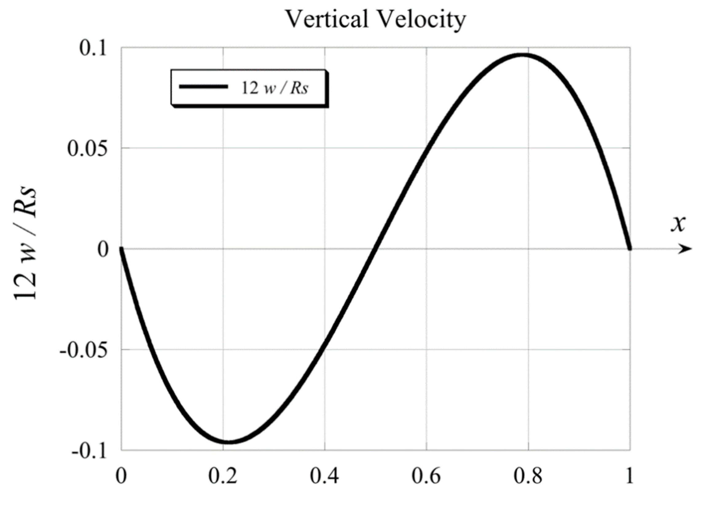
The vertical velocity solution obtained in Equation (50) shows that in addition to being zero at the boundaries $x=0$ and $x=1$ it has a third zero at $x=0.5$, evidence for a recirculating convective flow. The solution for the velocity expressed by Equation (50) is presented graphically in Figure 3 in terms of $12w/Rs$.

There is an anomaly in the solution for the mass fraction $C$ as the mass fraction can never be negative, but the solution (45) clearly produces negative values for the Soret numbers greater than 2. Therefore, for $So>2$ the solution (45) has no physical meaning. This restriction on the values that the Soret number can take is artificial, and it implies that the thermodiffusion coefficient must be allowed to vary with the mass fraction and can take negative values. The solution and the results of incorporating the latter in the model are presented in the next section.

Note that should we have used imposed mass fraction values on the boundaries, this anomaly would have been prevented, and the mass fraction values would fall in between the values imposed on the boundaries. For example, if the boundary conditions for the mass fraction would have been: for $x=0:\hspace{0.17em}\hspace{0.17em} C=C_h$ and for $x=1:\hspace{0.17em}\hspace{0.17em} C=C_l$ with $C_h>C_l>0$, then the solution to Equation (41) subject to these boundary conditions would have been $C=C_h\left(1-x\right)+C_{l}x$ and $C>0$ everywhere within the domain. Actually $C_l\le C\le C_h\hspace{0.17em}\hspace{0.17em}\hspace{0.17em}\forall \hspace{0.17em}x\in \left[0,1\right]$. However, as indicated in the introduction, imposing set values of the mass fraction on the boundaries is not practical, and it is most likely even impossible.

4. Method of Solution and Results for Mass Fraction Dependent and Possibly Negative Thermo-Diffusion Coefficient

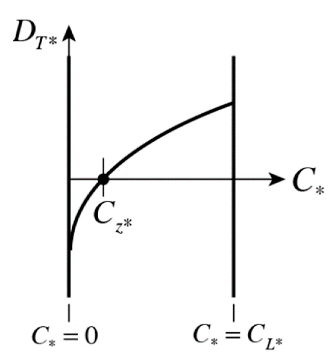
By allowing the thermodiffusion coefficient to vary with the mass fraction, including the possibility of taking negative values, we allow the possibility of the Soret effect to be weakened and even change direction (i.e., up the thermal gradient, from cold to hot regions) in places where the mass fraction is low and close to zero. A graph of such a mass-fraction-dependence is presented qualitatively in Figure 4 for a mass fraction within limits $0<C_{*}<C_{L*}$. Quantitative data have been presented by Köhler and Morozov [4], Geelhoed et al. [8], Jawad [9], Lapeira et al. [10], Yan et al. [12], and Mialdun et al. [14]. From Figure 4, it is evident that the thermodiffusion coefficient becomes negative for values of $C_{*}<C_{Z*}$, where $C_{Z*}$ is the value of mass fraction where the thermodiffusion coefficient is zero $D_{T*}=0$. One can represent this function as a linear approximation for a certain range of mass fraction values in the form:

$$D_{T*}=\left(C_{*}-C_{Z*}\right){\tilde{D}}_{T*},$$

(52)

where ${\tilde{D}}_{T*}$ is constant. Then the Soret number is redefined in terms of this constant value in the form:

$$So=\frac{{\tilde{D}}_{T*}\Delta T_{ch}}{D_{m*}}.$$

(53)

The mass flux consequently is reformulated in the form:

$${\mathit{j}}_{*}=-D_{m*}{\nabla }_{*}{C}_{*}-{\tilde{D}}_{T*}\left(C_{*}-C_{Z*}\right){\nabla }_{*}{T}_{*}$$

(54)

and, in the dimensionless form, it becomes:

$$j=-\nabla C-So\left(C-C_Z\right)\nabla T$$

(55)

converting Equation (17) to the form:

$$\frac{\partial \hspace{0.17em}C}{\partial \hspace{0.17em}t}+V·\nabla C=\frac{1}{L{e}_m}{\nabla }^{2}C+\frac{So}{L{e}_m}\nabla ·\left[\left(C-C_Z\right)\nabla T\right],$$

(56)

which subject to the assumptions of a steady-state, two-dimensional solution, and developed flow, developed temperature and developed mass fraction in the $z$-direction, and for the temperature solution obtained $T=x$, produces the following equation for the mass fraction from Equation (56):

$$\frac{{\mathrm{d}}^{2}C}{\mathrm{d}{x}^2}+So\frac{\mathrm{d}C}{\mathrm{d}x}=0$$

(57)

or

$$\frac{\mathrm{d}}{\mathrm{d}x}\left(\frac{\mathrm{d}C}{\mathrm{d}x}+So\hspace{0.17em}C\right)=0.$$

(58)

The solution to Equation (58) is obtained by a direct sequence of integrations in the form:

$$C=-\frac{A_1}{So}{\mathrm{e}}^{-So·\hspace{0.17em}x}+A_2.$$

(59)

The boundary conditions (29) and (30) are also modified by using the reformulated mass flux (55) and the solution for the temperature $T=x$ in the form

$$x=0:\hspace{0.17em}\hspace{0.17em} T=0\hspace{0.17em},\hspace{0.17em}\hspace{0.17em}\hspace{0.17em}{\left(\frac{\partial \hspace{0.17em}C}{\partial \hspace{0.17em}x}\right)}_{x=0}=-So\hspace{0.17em}{\left(C-C_Z\right)}_{x=0}\hspace{0.17em},\hspace{0.17em}\hspace{0.17em}\hspace{0.17em}w=0,$$

(60)

$$x=1:\hspace{0.17em} \hspace{0.17em}\frac{\partial T}{\partial x}=1\hspace{0.17em},\hspace{0.17em}\hspace{0.17em}\hspace{0.17em}\hspace{0.17em}{\left(\frac{\partial \hspace{0.17em}C}{\partial \hspace{0.17em}x}\right)}_{x=1}=-So\hspace{0.17em}{\left(C-C_Z\right)}_{x=1}\hspace{0.17em},\hspace{0.17em}\hspace{0.17em}\hspace{0.17em}w=0.$$

(61)

Consequently, the integration constant $A_2$ is evaluated by using these boundary conditions with the solution (59), leading to $A_2=C_Z$ and:

$$C=-\frac{A_1}{So}{\mathrm{e}}^{-So\hspace{0.17em}·x}+C_Z.$$

(62)

Again, one cannot determine the value of the integration constant $A_1$ from these boundary conditions, and we again apply the condition of conservation of the suspended particles (43) to determine this constant to yield:

$$A_1=-\frac{\left(1-C_Z\right)}{\left(1-{\mathrm{e}}^{-So}\right)}S{o}^2$$

(63)

and

$$C=\frac{\left(1-C_Z\right)So}{\left(1-{\mathrm{e}}^{-So}\right)}{\mathrm{e}}^{-So\hspace{0.17em}·x}+C_Z$$

(64)

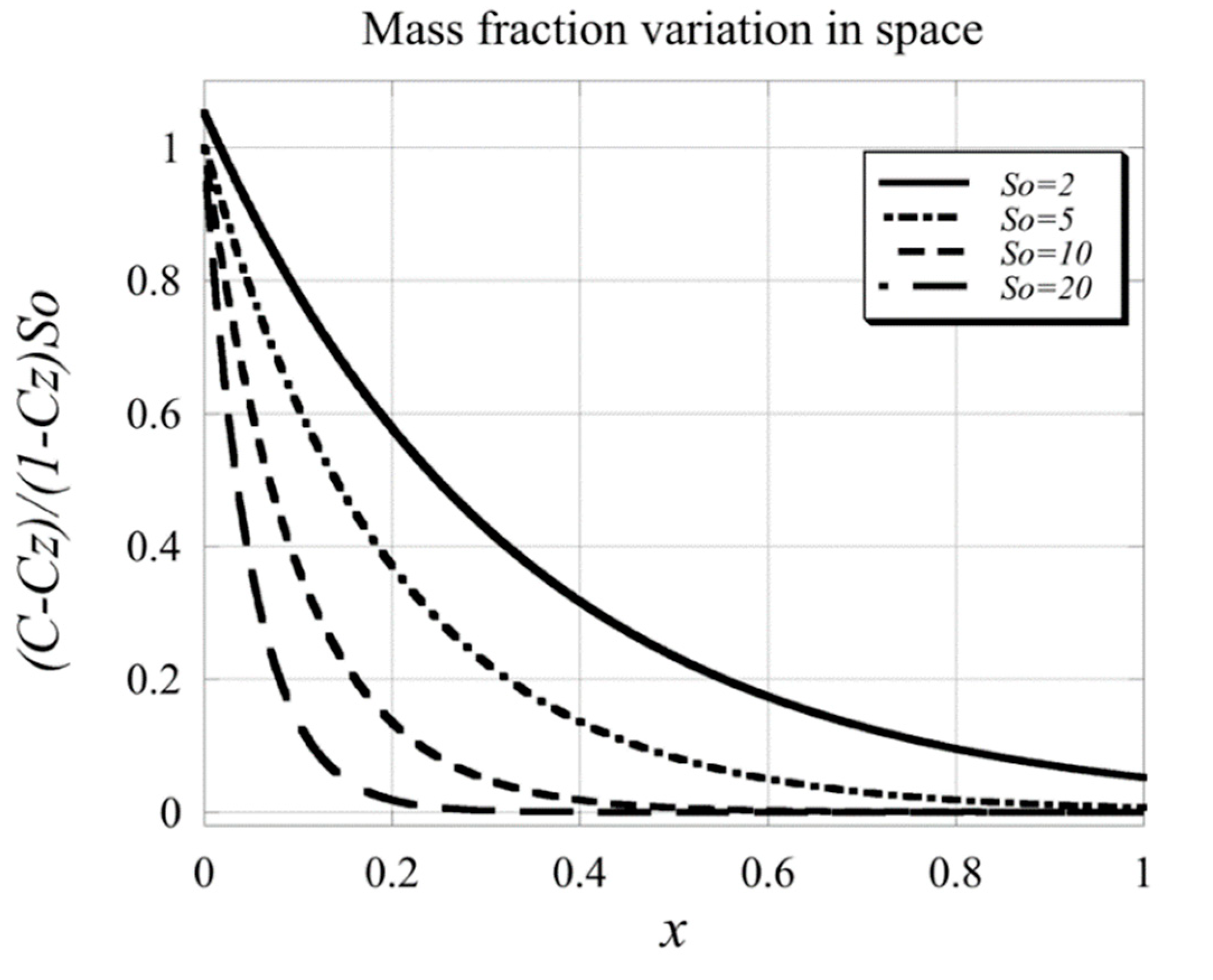
and it is now evident that the solution for the mass fraction is always positive for all values of the Soret number, i.e., $C>0$ for all $So>0$. Actually, in the limit $C\to C_Z$ as $So\to 0$ and $C\to C_Z$ as $So\to \infty$. The graphical representation of the solution (64) in terms of $\left(C-C_Z\right)/\left(1-C_Z\right)So$ as a function $x$ is presented in Figure 5.

Note that $C_Z$ does not have to be positive for the solution of the mass fraction $C$ to remain positive. Actually, as long as:

$$C_Z>\hspace{0.17em}\hspace{0.17em}-\hspace{0.17em}\hspace{0.17em}\frac{So}{\left[{\mathrm{e}}^{So}-\left(So+1\right)\right]},$$

(65)

the mass fraction is always positive. $C_Z$ is not an actual value of mass fraction. It stands only to describe the variation of the thermodiffusion coefficient. For the linear function (52) considered here, a more negative value of $C_Z$ implies a stronger positive Soret effect at low mass fractions. This last result demonstrates that it is not the nonlinearity that removed the anomaly as for values of $C_Z$ not satisfying inequality (65), the solution for the mass fraction would still be negative. It is rather the specific characteristic of the thermodiffusion coefficient, which causes weaker (or even negative) Soret effects in regions of the low mass fraction that removed the anomaly and rendered the solution into a physically meaningful form.

Substituting the solution for the mass fraction (64) and for the temperature (40) into Equation (35) leads to:

$$\hspace{0.17em}\frac{{\mathrm{d}}^2\hspace{0.17em}w}{\mathrm{d}\hspace{0.17em}{x}^2}=P_z-R{a}_T\hspace{0.17em}x+\frac{R{a}_C}{L{e}_m}\left[\frac{\left(1-C_Z\right)So}{\left(1-{\mathrm{e}}^{-So}\right)}{\mathrm{e}}^{-So\hspace{0.17em}·x}+C_Z\right].$$

(66)

Integrating twice this equation and using the boundary conditions (60) and (61), stating that $w=0$ at $x=0$ and $x=1$ yields a solution in terms of the yet undetermined constant $P_z$. Applying the condition (48) of no flowrate over any cross-section, i.e., ${\displaystyle {\int }_0^{1}w\mathrm{d}x}=0$ leads to the determination of $P_z$ and produces the solution for the vertical velocity in the form:

$$\hspace{0.17em}\frac{w}{R{a}_T}=\frac{1}{2}x\left(x-1\right)\left[\left(\frac{P_z}{R{a}_T}+R_{TC}{C}_Z\right)-\frac{1}{3}\left(x+1\right)\right]+R_{TC}\frac{\left(1-C_Z\right)}{So}\left[x-\frac{\left(1-{\mathrm{e}}^{-So\hspace{0.17em}x}\right)}{\left(1-{\mathrm{e}}^{-So}\right)}\right],$$

(67)

where

$$R_{TC}=\frac{R{a}_C}{L{e}_{m}R{a}_T}=\frac{{\beta }_{C*}{C}_o}{{\beta }_{T*}\Delta T_{ch}}$$

(68)

and

$$\left(\frac{P_z}{R{a}_T}+R_{TC}{C}_Z\right)=\frac{1}{2}+\frac{6R_{TC}\left(1-C_Z\right)}{S{o}^2}\left[\frac{\left(2-So\right)-\left(2+So\right){\mathrm{e}}^{-So}}{\left(1-{\mathrm{e}}^{-So}\right)}\right].$$

(69)

The limit of Equation (69) as $So\to \infty$ is simply obtained in the form:

$$\underset{So\to \infty }{\lim }\left(\frac{P_z}{R{a}_T}+R_{TC}{C}_Z\right)=\frac{1}{2}$$

(70)

that being substituted into Equation (67), produces:

$$\hspace{0.17em}\underset{So\to \infty }{\lim }\left(\frac{w}{R{a}_T}\right)=-\frac{1}{6}x\left(x-1\right)\left(x-\frac{1}{2}\right)$$

(71)

showing that velocity also vanishes at $x=0.5$, in addition to vanishing on the boundaries at $x=0$ and $x=1$.

The limit of Equation (69) as $So\to 0$ is obtained by applying the L’Hopital rule to obtain:

$$\underset{So\to 0}{\lim }\left(\frac{P_z}{R{a}_T}+R_{TC}{C}_Z\right)=\frac{1}{2}$$

(72)

that being substituted into Equation (67), produces, after applying L’Hopital rule, the same solution as for $So\to 0$, i.e.,

$$\hspace{0.17em}\underset{So\to 0}{\lim }\left(\frac{w}{R{a}_T}\right)=-\frac{1}{6}x\left(x-1\right)\left(x-\frac{1}{2}\right).$$

(73)

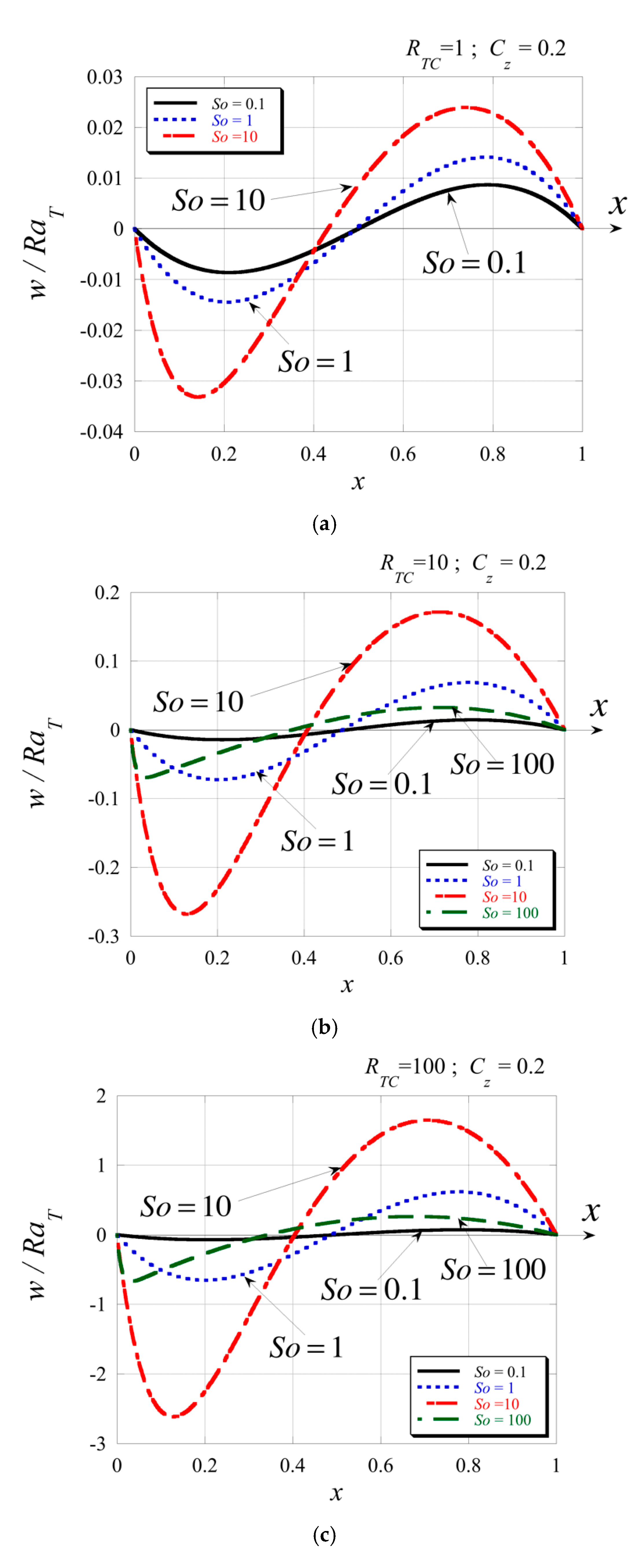
Therefore, the non-boundary zero of the velocity is located at $x=0.5$ in both limits of the Soret number, i.e., for $So\to \infty$, and for $So\to 0$. The graphical representation of the solution (67) for the velocity profile in terms of $w\left(x\right)/R{a}_T$ is shown in Figure 6 for a constant value of $C_Z=0.2$ and for different values of the Soret number and different values of $R_{TC}$. Each graph in Figure 6 corresponds to a constant value of $R_{TC}$ while the curves belong to different values of $So$. By comparing the graphs, it seems that increasing the value of $R_{TC}$ enhances the strength of the convective flow, while comparing the curves on each graph shows that generally increasing the Soret number also increases the strength of the convective flow, but up to a limit. From Figure 6bc, it is evident that the flow at $So=100$ is substantially weaker than the flow at lower values of the Soret number, reversing the enhancing trend of the impact of the $So$ number on the flow for lower values of the Soret number.

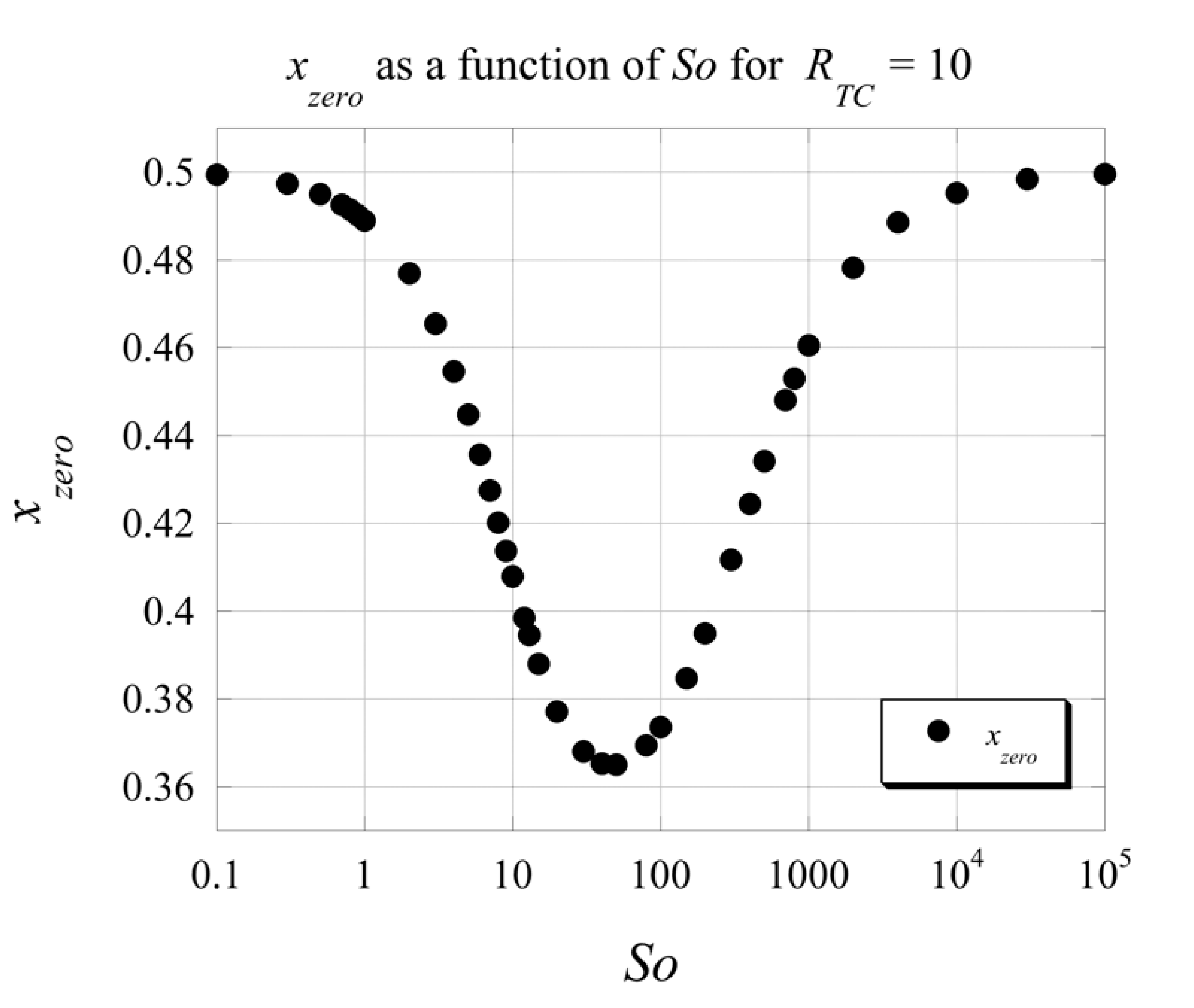
From Figure 6, one can also observe that the location of the non-boundary zero of the velocity varies with changing the value of the Soret number. To clarify this point further, we present the velocity profiles in Figure 7 by keeping each graph at a constant value of $So$ and showing the variation due to changing the value of $R_{TC}$. From the graphs, it is evident that the value of $R_{TC}$ does not affect the location of the non-boundary zero of the velocity, while the $So$ number controls its location. Increasing the value of $R_{TC}$ increases the strength of the flow, as does increasing the Soret number up to a value of $So=10$. Beyond this value, as it can be observed from Figure 7e, associated with $So=100$ the strength of the flow becomes weaker again.An evaluation to investigate further the impact of the Soret number on the location of the non-boundary zero of the velocity led to results of this location as a function of $So$ number as presented in Figure 8 with the Soret axis on a logarithmic scale, for $R_{TC}=10$ and $C_Z=0.2$. Since we noticed from Figure 7 that the values of $R_{TC}$ do not affect this location selecting $So$ as the variable parameter seems adequate. From Figure 8, it is evident that for the Soret number values lower than 50, the location of the non-boundary zero moves from 0.5 at $So\to 0$ ($So=0.1$) to ~0.364 at about $So\sim 50$ and then increases again as the Soret number increases beyond 50, reaching the value of 0.5 again when $So\to \infty$ ($So={10}^5$). This result is consistent with the limits we evaluated analytically previously.

5. Conclusions

A more realistic boundary condition for the mass fraction of a binary mixture is being considered in this paper since setting specified arbitrary values of the mass fraction (or solute concentration) on the boundaries is extremely difficult, if not impossible, to accomplish experimentally. This more realistic boundary condition for the mass fraction (solute concentration) is a zero-flux that accounts for thermodiffusion via thermophoresis (Soret effect). The problem of natural convection in a binary mixture subject to this realistic boundary conditions of imposed zero mass flux on the solid walls shows solutions that may lead to unrealistic negative values of the mass fraction (or solute concentration). This anomaly is being investigated in the present paper, and a possible way of addressing it is suggested via a mass-fraction-dependent thermodiffusion coefficient that can have negative values in regions of low mass fractions. The solution to the basic convection problem by using such mass-fraction-dependent thermodiffusion coefficient shows that the anomaly of negative mass fractions is removed. Further analysis of the solution is undertaken to identify limits for the strength and shape of the recirculating convective flow.

References

- Brand, H.R.; Hohenberg, P.C.; Steinberg, V. Codimension-2 bifurcations for convection in binary fluid mixtures. Phys. Rev. A 1984, 30, 2549–2561. [Google Scholar] [CrossRef]
- Bird, R.B.; Stewart, W.E.; Lightfoot, E.N. Transport Phenomena; John Wiley and Sons: New York, NY, USA, 1960. [Google Scholar]
- Hollinger, S.T.; Lüke, M. Influence of the Dufour effect on convection in binary gas mixtures. Phys. Rev. E 1995, 52, 642–657. [Google Scholar] [CrossRef] [PubMed] [Green Version]
- Köhler, W.; Morozov, K.I. The Soret effect in liquid mixtures—A review. J. Non Equilib. Thermodyn. 2016, 41, 151–197. [Google Scholar] [CrossRef]
- Mortimer, R.G.; Eyring, H. Elementary transition state theory of the Soret and Dufour effects. Proc. Natl. Acad. Sci. USA 1980, 77, 1728–1731. [Google Scholar] [CrossRef] [PubMed] [Green Version]
- Postelnicu, A. Influence of a magnetic field on heat and mass transfer by natural convection from vertical surfaces in porous media considering Soret and Dufour effects. Int. J. Heat Mass Transf. 2004, 47, 1467–1472. [Google Scholar] [CrossRef]
- Weaver, J.A.; Viskanta, R. Natural convection due to horizontal temperature and concentration gradients-2. Species interdiffusion, Soret and Dufour effects. Int. J. Heat Mass Transf. 1991, 34, 3121–3133. [Google Scholar] [CrossRef]
- Geelhoed, P.; Westerweel, J.; Kjelstrup, S.; Bedeaux, D. Thermophoresis. In Encyclopedia of Microfluidics and Nanofluidics; Li, D., Ed.; Springer: Boston, MA, USA, 2008. [Google Scholar]
- Jawad Hussam, K. Natural Convection and Soret Effect in a Multi-Layered Liquid and Porous System, Paper 1512 Digital Commons @ Ryerson. Master’s Thesis, Ryerson University, Toronto, ON, Canada, 2012. [Google Scholar]
- Lapeira, E.; Bou-Ali, M.M.; Madariaga, J.A.; Santamaria, C. Thermodiffusion coefficients of water/ethanol mixtures for low water mass fractions. Microgravity Sci. Technol. 2016, 28, 553–557. [Google Scholar] [CrossRef]
- Madariaga, J.A.; Santamaria, C.; Bou-Ali, M.M.; Urteaga, P.; Alonso De Mezquia, D. Measurement of thermodiffusion coefficient in n-Alkane binary mixtures: Composition dependence. J. Phys. Chem. 2010, 114, 6937–6942. [Google Scholar] [CrossRef] [PubMed]
- Yan, Y.; Blanco, P.; Saghir, M.Z.; Bou-Ali, M.M. An improved theoretical model for thermal diffusion coefficient in liquid hydrocarbon mixtures: Comparison between experimental and numerical results. J. Chem. Phys. 2008, 129, 194507. [Google Scholar] [CrossRef] [PubMed]
- Costesèque, P.; Mojtabi, A.; Platten, J.K. Thermodiffusion phenomena. C. R. Mécanique 2011, 339, 275–279. [Google Scholar] [CrossRef] [Green Version]
- Mialdun, A.; Yasnou, V.; Shevtsova, V.; Koniger, A.; Kohler, W.; Alonso de Mezquia, D.; Bou-Ali, M.M. A comprehensive study of diffusion, thermodiffusion, and Soret coefficients of water-isopropanol mixtures. J. Chem. Phys. 2012, 136, 244512. [Google Scholar] [CrossRef]
- Chipman, J. The Soret effect. J. Am. Chem. Soc. 1926, 48, 2577–2589. [Google Scholar] [CrossRef]
- Klein, M.; Wiegand, S. The Soret effect of mono- di- and triglycols in ethanol. Phys. Chem. Chem. Phys. 2011, 13, 7090–7094. [Google Scholar] [CrossRef] [PubMed] [Green Version]
- Putnam, S.A.; Cahill, D.G.; Wong, G.C.L. Temperature dependence of thermodiffusion in aqueous suspensions of charged nanoparticles. Langmuir 2007, 23, 9221–9228. [Google Scholar] [CrossRef] [PubMed]
- Duhr, S.; Braun, D. Why molecules move along a temperature gradient. Proc. Natl. Acad. Sci. USA 2006, 103, 19678–19682. [Google Scholar] [CrossRef] [PubMed] [Green Version]
- Mojtabi, A.; Platten, J.K.; Charrier-Mojtabi, M.C. Onset of free convection in solutions with variable Soret coefficients. J. Non Equilib. Thermodyn. 2002, 27, 25–44. [Google Scholar] [CrossRef] [Green Version]
- Gorban, A.N.; Sargsyan, H.P.; Wahab, H.A. Quasichemical models of multicomponent nonlinear diffusion. Math. Model. Nat. Phenom. 2011, 6, 184–262. [Google Scholar] [CrossRef] [Green Version]
- Boussinesq, J. Theorie Analitique de la Chaleur; Gutheir-Villars: Paris, France, 1903; Volume 2, p. 172. [Google Scholar]
- Vadasz, P. Fluid Flow and Heat Transfer in Rotating Porous Media; Springer International Publishing AG: Cham, Switzerland, 2015. [Google Scholar] [CrossRef]
Figure 1.
A vertical tall, fluid layer consisting of a binary mixture, heated by a constant heat flux on one side and exposed to a constant low temperature on the other side.
Figure 2.
Graphical profile of the solution for (a) the basic temperature and (b) the basic mass fraction.
Figure 3.
Graphical profile of the solution for the vertical velocity.
Figure 4.
Qualitative description of the mass-fraction-dependent thermodiffusion coefficient, including negative values.
Figure 5.
Graphical profile of the solution for the basic mass fraction for different Soret numbers.
Figure 6.
Graphical profiles of the velocity solution for and different Soret numbers: (a) , (b): , and (c) .
Figure 7.
Graphical profiles of the velocity solution for and different values of : (a) , (b) , (c) , and (d) .
Figure 8.
The variation of the location of the non-boundary zeros of the velocity with the Soret number .
Publisher’s Note: MDPI stays neutral with regard to jurisdictional claims in published maps and institutional affiliations. |
© 2021 by the author. Licensee MDPI, Basel, Switzerland. This article is an open access article distributed under the terms and conditions of the Creative Commons Attribution (CC BY) license (http://creativecommons.org/licenses/by/4.0/).
Share and Cite
MDPI and ACS Style
Vadasz, P. A Hidden Anomaly in the Binary Mixture Natural Convection Subject to Flux Boundary Conditions. Physics 2021, 3, 144-159. https://doi.org/10.3390/physics3010012
AMA Style
Vadasz P. A Hidden Anomaly in the Binary Mixture Natural Convection Subject to Flux Boundary Conditions. Physics. 2021; 3(1):144-159. https://doi.org/10.3390/physics3010012
Chicago/Turabian StyleVadasz, Peter. 2021. "A Hidden Anomaly in the Binary Mixture Natural Convection Subject to Flux Boundary Conditions" Physics 3, no. 1: 144-159. https://doi.org/10.3390/physics3010012